Hyperparameter Sensitivity in Deep Outlier Detection
Analysis and a Scalable Hyper-Ensemble Solution

Abstract

Outlier detection (OD) literature exhibits numerous algorithms as it applies to diverse domains. However, given a new detection task, it is unclear how to choose an algorithm to use, nor how to set its hyperparameter(s) (HPs) in unsupervised settings. HP tuning is an ever-growing problem with the arrival of many new detectors based on deep learning, which usually come with a long list of HPs. Surprisingly, the issue of model selection in the outlier mining literature has been “the elephant in the room”; a significant factor in unlocking the utmost potential of deep methods, yet little said or done to systematically tackle the issue. In the first part of this paper, we conduct the first large-scale analysis on the HP sensitivity of deep OD methods, and through more than 35,000 trained models, quantitatively demonstrate that model selection is inevitable. Next, we design a HP-robust and scalable deep hyper-ensemble model called RobOD that assembles models with varying HP configurations, bypassing the choice paralysis. Importantly, we introduce novel strategies to speed up ensemble training, such as parameter sharing, batch/simultaneous training, and data subsampling, that allow us to train fewer models with fewer parameters. Extensive experiments on both image and tabular datasets show that RobOD achieves and retains robust, state-of-the-art detection performance as compared to its modern counterparts, while taking only $2$-$10$% of the time by the naïve hyper-ensemble with independent training.

1 Introduction

Outlier detection (OD) finds numerous real-world applications in finance, security, healthcare, to name a few. Thanks to this popularity, the literature has grown to offer a large catalog of detection algorithms [1]. With the recent advances in deep learning, the literature has been booming with the addition of many more OD models based on deep neural networks (NNs). (See surveys [9, 31, 36].)

While there is no shortage of OD methods today, given a new task, it is unclear how to choose which algorithm or model to use, nor how to configure its hyperparameter(s) (HPs) in unsupervised settings. That is, the fundamental problem of outlier model selection remains vastly understudied. Several evaluation studies have illustrated the sensitivity to HPs for traditional (i.e. non-deep) OD methods [2, 8, 17]. Most surprisingly, however, the issue of HP tuning/model selection for the newly burgeoning deep OD models has been “the elephant in the room”; a well-known problem that no one seems to want to bring up, which is exactly the focus of this paper.

Deep OD models are promising thanks to appealing properties such as task-driven representation learning and end-to-end optimization. On the other hand, while their traditional counterparts had only 1-2 HPs, deep OD models come with a long list of HPs: ($i$) architecture HPs (e.g. depth, width), ($ii$) regularization HPs (e.g. dropout, weight decay rates), and ($iii$) optimization HPs (e.g. learning rate, epochs). These are inherited ones from regular deep NNs while most also exhibit their model-specific/specialized HPs. It would not be a freak occurrence to assume that their performance is heavily dependent on these HP settings. However, our closer analysis of the experiment testbeds in recent literature on deep OD models falls far from systematically addressing the issue. (See Appx. A.1 Table 8 for a preview.) We find hardly any discussion on model selection, with only a few work empirically studying sensitivity but to model-specific HPs only. Majority of work report results for a single “recommended” (how, unclear) configuration used for all datasets, or tune only a subset of the HPs on labeled validation and sometimes even test (!) data. To the best of our knowledge, there is no existing work that attempts (unsupervised) model selection for deep OD models.

In this work, our research goals are two-fold. First, through extensive experiments, we quantitatively demonstrate that deep OD models from various families are all sensitive to their HP settings. Our analysis shows that model selection is inevitable and is key to truly unlock the utmost potential of deep OD models. Second, motivated by our analysis, we propose a scalable deep hyper-ensemble called RobOD that obviates HP selection through assembly of deep autoencoders with varying HP configurations. To speed up ensemble training, we introduce novel architectural and training strategies, and train fewer models, with fewer parameters, on smaller subsamples of data; by leveraging parameter sharing and joint/simultaneous training. The main contributions of our work are as follows.

• First large-scale study on HP sensitivity of deep OD models:  We build a large testbed to systematically measure the performance variability of deep OD models under varying HP settings. Our study involves models from four different families, on both image and vector data, under both “clean” (i.e. inlier only) as well as “polluted” (i.e. outlier-contaminated) training data, over 3 random initializations, 80-800+ different HP configurations per model across 4-8 unique HPs. Overall, our analysis involves more than 35,000 runs. (Sec. 3)

• RobOD, a new deep hyper-ensemble OD model:  Motivated by our empirical study, we propose a hyper-ensemble model called RobOD which combines scores from a collection of models, each trained with a different HP configuration. Rather than trying to choose, RobOD fully bypasses the choice of and hence sensitivity to HP settings, and achieves robust (i.e. stable) performance across different initializations. (Sec. 4.1)

• Design strategies to speed up hyper-ensemble training:  We propose speed-up strategies to efficiently hyper-ensemble model depth and width. We use an autoencoder (AE) with skip-connections to simultaneously train multiple AEs with different depths. In addition, we employ batch training of multiple models and use zero-masking on shared parameters to get different widths. Together, these provide a 90-98$\%$ savings in running time. (Sec. 4.2)

• Extensive experiments:  Besides our large-scale measurement study, we also perform experiments on additional benchmark datasets, comparing RobOD to baseline deep OD models as well as a traditional tree-ensemble. RobOD achieves competitive or often better performance which, importantly, exhibits low variance by random initialization. (Sec. 5)

We expect that our work will increase awareness and help shift the community’s focus (at least to some extent) from building the next yet-another deep OD model toward the fundamental issue of unsupervised model selection and hyperparameter-robust model design. To foster future research, we open source all code and datasets at https://github.com/xyvivian/ROBOD.

2 Related Work

Unsupervised Outlier Detection (OD).  There exists a large pool of what-is-now-called traditional, i.e. not deep learning based, OD methods [1, 10]. These methods work with the original features or subspaces thereof, and typically exhibit just one or two hyperparameters (HPs). With recent advances in deep learning, there has been a boom in deep OD models, as those can learn new task-dependent feature representations and directly optimize an OD objective. Despite their short history, multiple surveys have been published that aim to cover this fast-growing literature [9, 31, 36]. While deep OD models have been shown to outperform their traditional counterparts, they exhibit a much longer list of (typically 4-8) HPs (e.g. depth, width, dropout, weight decay, learning rate, epochs, etc. besides other model-specific HPs) that makes them very challenging to tune in unsupervised settings.

Model Selection in Unsupervised OD: Prior (Black) Art.  At large, unsupervised outlier model selection remains to be a vastly understudied, yet extremely important area. Various evaluation studies have reported traditional detectors to be quite sensitive to their HP choices [2, 8, 17], raising concern for the fair evaluation and comparison of different models. Earlier work on automatically selecting HPs are limited to one-class models [14, 40, 41]. More recently, general-purpose internal (i.e., unsupervised) model evaluation heuristics have been proposed [15, 29, 30], which solely rely on the input data (without labels) and the output (i.e., outlier scores). MetaOD [47] employs meta-learning to transfer information from similar historical tasks to a new task for model selection, which has only been tested on traditional OD models. Different from those that aim to select a single model, ensemble models have also been employed for OD [3], including those that combine models from the same family [26] as well as heterogeneous detectors from different families [33].

Regarding deep OD methods, we have surveyed a large collection of recent papers and their experimental testbed and HP settings, a summary of which is given in Appx. A.1 Table 8. To our surprise, we found hardly any discussion on model selection, with only a few work presenting sensitivity analysis with respect to not all but some, model-specific HPs. While some work reserve labeled validation/hold-out data to tune a subset of the HPs [6, 18, 23], majority of them fix the HP values and call them “recommended”/default settings [5, 11, 37, 38, 46, 49]. Moreover, a non-negligible number of existing work choose some critical HPs empirically on test data (!) to yield optimum results [4, 35, 48] (See Table 8, last column). Some work that builds on previous models (e.g., deep SVDD-based methods [35] vs. multi-sphere extension [13], transformation-based methods [16] for images vs. their extension to vector data [5], AnoGAN [37] and the follow-up EGBAD [46]) use the same architecture and HP settings as the prior work for consistent/“fair” comparison. However it is unlikely that the same HP values would work comparably for different models.

Admittedly, it is challenging to tune (a long list of) HPs in the absence of labels, yet, the opacity in the deep OD literature warrants careful investigation on the stability of model performance under varying HP settings, and ultimately on the fair comparison between these and traditional OD methods.

Deep Model Ensembles.  Recently, deep NN predictions have been found to be often poorly calibrated [20]. As Bayesian learning does not offer straightforward training, deep ensemble models have been proposed as a simple alternative [25] to improve predictive uncertainty, as well as efficient ways of training deep NN ensembles [19, 42]. In this work, we leverage ensemble modeling toward a different goal: to improve the stability and robustness of unsupervised OD models to HP settings, combining predictions from models with different HPs into an OD hyper-ensemble. The closest to our work is Wenzel et al.’s deep hyper-ensemble [43], which, different from ours, considers supervised problems, to further foster diversity in the ensemble and thereby achieve better uncertainty estimation.

3 Hyperparameter-Sensitivity Analysis of Deep OD

3.1 Testbed Setup

Models. We study HP sensitivity of five deep OD methods of four different types: a basic deep autoencoder VanillaAE trained with reconstruction loss, robust deep autoencoder RDA [48], one-class classification based DeepSVDD [35], adversarial training based GANomaly [4], and an (AE) ensemble model RandNet [11]. These exhibit 4 to 8 HPs, as listed in Table 1. (See Appx. A.2 for descriptions.) (Note that RandNet is not a hyper-ensemble: members use the same HP configs except for NN sparsity.) We define a grid of 2-3 different values for each HP, including the author-recommended values when available (See details in Appx. Table 9), and train each deep OD method with all combinations; yielding 81-864 different models. (Note that 192 RandNet models each consists of an ensemble of 50 or 200 AEs.) We repeat each experiment 3 times with different initializations.

Table 1: Deep OD models used for studying hyperparameter sensitivity. We give the number (in parenthesis) and the list of HPs for each method, along with the total number of models trained for evaluation. (See Appx. A.2 for HP descriptions and Appx. Table 9 for list of grid values per HP.)

Method	List of hyperparameters (HPs)	#models
VanillaAE	(4) n_layers $\cdot$ layer_decay $\cdot$ LR $\cdot$ iter	81
RDA [48]	(6) $\lambda$ $\cdot$ n_layers $\cdot$ layer_decay $\cdot$ LR $\cdot$ inner_iter $\cdot$ iter	324
DeepSVDD [35]	(8) conv_dim $\cdot$ fc_dim $\cdot$ Relu_slope $\cdot$ pretr_iter $\cdot$ pretr_LR $\cdot$ iter $\cdot$ LR $\cdot$ wght_dc	864
GANomaly [4]	(6) $w_{adv}=1$ $\cdot$ $w_{con}$ $\cdot$ $w_{enc}$ $\cdot$ z_dim $\cdot$ LR $\cdot$ iter	162
RandNet [11]	(8) n_layers $\cdot$ layer_decay $\cdot$ sample_r $\cdot$ ens_size $\cdot$ pretr_iter$=100$ $\cdot$ iter $\cdot$ LR $\cdot$ wght_dc$=0$	192

Train/Test settings. In their original papers, DeepSVDD and GANomaly are trained on what we refer to as Clean (inlier only) data, and tested on a disjoint test dataset. In contrast, RDA and RandNet consider the transductive setting where the train data is the same as the test data, containing inliers as well as outliers, which we refer to as Polluted. It is often understood to be more challenging than the Clean setting for unsupervised OD. For completeness, we evaluate these methods under both settings.

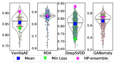
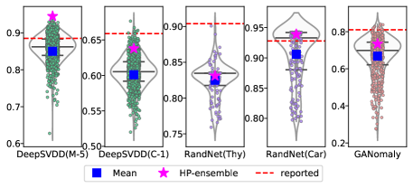
Figure 1: (left) AUROC performance of deep OD methods with different HP configurations (circles) on MNIST-4 showcase notable variation (i.e., sensitivity). (See footnote 2 below.) (right) Similar results on additional datasets; DeepSVDD on MNIST-5 and CIFAR10-auto, RandNet on Thyroid and Cardio, and GANomaly on MNIST-4out. Reported values (dashed lines) are overestimates of Mean ($\square$). Hyper-ensemble (☆) improves notably over Mean.

Datasets.  For evaluation we consider both image point datasets. As in the original papers [4, 35], we use MNIST and CIFAR10 to construct OD tasks, except for RandNet which uses fully-connected rather than convolutional layers and is originally tested only on point-cloud benchmarks.

Metrics.  Across all HP settings of a deep OD method, we report the mean AUROC, standard deviation (stdev), as well as minimum and maximum. Mean corresponds to the expected performance when a HP config is randomly picked from our (multi-dimensional) grid. We also report the average mean and its stdev over 3 repeated runs. For datasets that are directly comparable to those in the original papers, we contrast the mean model performance that we obtain to that reported value for author-recommended HPs. We compare to a simple model (i.e. HP) selection heuristic, which selects the (one) model with the lowest loss/objective value. In addition, instead of selecting one, we average the scores from all configurations and report the AUROC of this hyper-ensemble.

Over five deep OD methods, tens to hundreds of HP configs, multiple initializations, Clean and Polluted settings, and various datasets, we have trained a total of more than 35,000 models. As such, our study constitutes the first large-scale HP sensitivity analysis in the deep outlier mining literature.

3.2 Results and Observations

Fig. 1(left) provides the AUROC performances for VanillaAE, RDA, DeepSVDD and GANomaly across all HP configurations (circles), for the Polluted setting (See Appx. A.3 Fig. 6 for Clean setting.) on MNIST-4 dataset where digit ‘4’ images are designated as inliers and the rest nine classes are down-sampled at 10% as outliers, as in the DeepSVDD paper [35]. Horizontal bars mark the 1st, 2nd (i.e. median), and 3rd quartiles, square the mean AUROC across HPs, triangle the selected model by lowest loss, and star the AUROC of the hyper-ensemble. (Corresponding plots over 3 runs per method are in Appx. A.3 Fig. 7.) Table 2 provides summary statistics as well as the hyper-ensemble performance for comparison for both the (left) Clean and (right) Polluted settings.

First, in Fig. 1 we observe that all methods exhibit notable variability in performance across HPs, with many worse-than-average configurations; e.g. for GANomaly, as well as many better-than-average models; e.g. for RDA. Mean performance is considerably lower than the best model’s, illustrating the opportunity or room for improvement. As one would expect, the performances in Table 2 are lower in the Polluted setting as compared to Clean (less so for the robust RDA), while sensitivity (i.e. stdev) is comparable or only slightly higher; showing that HP choice is critical under both settings.

We also find that selecting a model by the value of loss ($\triangledown$), despite requiring to train and choose from all models, often is much worse than the mean, i.e. random picking a (single) model ($\square$); proving this simple heuristic ineffective. On the other hand, the hyper-ensemble (☆) outperforms the mean in all cases, with quite small standard deviation across runs (i.e. low sensitivity to initialization).

The reported performance ($0.949\pm 0.008$) of DeepSVDD on MNIST-4 (under Clean) [35] is similar yet somewhat optimistic over the mean value we obtain. MNIST-4 is an easy task for DeepSVDD since mean AUROC is already around $0.924$. Thus, we set up MNIST-5 (with digit ‘5’ as inliers) with reported AUROC $0.885\pm 0.009$, as well as CIFAR10-auto (with class ‘automobile’ as inliers) (in both cases rest of the classes are subsampled at 10% each as outliers) with reported AUROC $0.659\pm 0.021$. We run DeepSVDD on both datasets under all 864 configurations. As shown in Fig. 1 (right), our mean AUROCs are $0.857\pm 0.037$ for MNIST-5, and $0.605\pm 0.024$ for CIFAR10-auto. (See Appx. A.3 Fig. 8 for all 3 runs.) The reported performances for the “recommended” HPs in DeepSVDD (dashed red lines) appear to be optimistic over the mean, i.e. what one would expect by random choice (in the absence of any labels or other strategies).

Table 2: Basic stats of AUROC ($\%$) distribution over varying HPs on MNIST-4 under (left) Clean and (right) Polluted settings. There is significant gap between the best and worst HP settings, with notable stdev around the mean. Polluted results have lower mean, and comparable or slightly higher variance. Hyper-ensemble outperforms random choice (i.e. mean), with low variability by initialization.

Method	Min&Max		Mean&Std.	Mean (avg. 3 runs)	Hyper-ens. Mean (avg. 3 runs)	Min&Max		Mean&Std.	Mean (avg. 3 runs)	Hyper-ens. Mean (avg. 3 runs)
Vanilla AE	87.41	98.19	93.12$\pm$2.91	93.12$\pm$0.008	95.30$\pm$0.03	76.34	91.20	85.73$\pm$2.95	85.76$\pm$0.08	90.46$\pm$0.12
RDA	81.79	95.96	88.94$\pm$2.43	88.95$\pm$0.02	89.39$\pm$0.02	62.29	93.35	86.30$\pm$3.68	86.24$\pm$0.06	86.82$\pm$0.04
DeepSVDD	75.75	96.58	92.39$\pm$2.02	92.37$\pm$0.02	95.94$\pm$0.05	67.54	91.71	81.65$\pm$4.15	81.66$\pm$0.10	93.07$\pm$0.70
GANomaly	17.49	95.73	78.90$\pm$16.63	78.26$\pm$0.51	86.87$\pm$0.31	29.06	86.60	67.20$\pm$10.30	67.45$\pm$0.32	73.87$\pm$0.52

The optimistic reporting trend holds for GANomaly and RandNet as well. Following their original paper [4], and different from [35], we set up MNIST-4out dataset to contain digit ‘4’ images this time as the outliers and the rest nine classes as inliers. GANomaly performances across 162 HP configs are shown in Fig. 1 (right), where the reported result (red line) in [4] of AUROC $0.795$ appears notably higher than the mean $0.668\pm 0.105$ that we obtain. (See Appx. A.3 Fig. 9 for all 3 runs.)

For RandNet, we first find and verify a third-party implementation, as the authors could not publicly share theirs, by replicating similar performances to those reported in [11] using the author-recommended HP settings on all 8 datasets. Then for Cardio and Thyroid datasets, we train 192 RandNet ensembles with varying HPs under Polluted as in the original paper. Results from one run are shown in Fig. 1 (right). (See Appx. A.3 Fig. 10 for all 3 runs.) On Cardio, AUROC mean is $0.894\pm 0.045$ vs. $0.929$ (reported), and Thyroid mean is $0.822\pm 0.026$ vs. $0.904$ (reported).

In summary, the take-aways from our analysis are as follows. First, it is clear that deep OD models are sensitive to their HP settings, showing that model/HP selection is inevitable. The mean/expected value (of random choice) can be quite away from the best model, motivating this line of research. Second, the recommended settings in recent deep OD papers are arguably optimistic; otherwise more transparency into their selection mechanism is warranted. Finally, hyper-ensemble performance is superior to the mean, possibly owing to different HPs implicitly imposing diversity among constituent models which helps improve detection. Besides performance improvement, hyper-ensembling obviates model selection by joining all models rather than choosing one and is not much sensitive to initialization – setting the stage for our proposed HP-robust OD method RobOD.

4 RobOD: A Deep Hyper-ensemble for Hyperparameter-Robust OD

4.1 Motivation and Overview

The main research question we consider is RQ1) how to design an unsupervised deep OD model that is robust to its HPs, i.e. an OD method that has stable, low-variance predictions under varying HPs. Motivated by our sensitivity analysis in Sec. 3, we propose a deep autoencoder (AE) hyper-ensemble model that combines scores from AE models with different HP configurations.

Definition 4.1 (Hyper-ensemble)

Given a model family $\mathcal{M}$ with $H$ HPs, let $\bm{\lambda}\in\mathbb{R}^{H}$ denote a specific setting of the HPs. A hyper-ensemble averages the output (outlier scores) from a finite number of base models with $m$ different config.s, i.e. $\frac{1}{m}\sum_{i=1}^{m}\mathcal{M}(\mathbf{x};\bm{\lambda}_{i})$ for point $\mathbf{x}$.

Hyper-ensembles exhibit multiple advantages. First, and to our end goal, they ease the model/HP selection burden, bypassing the “choice paralysis”. They are less sensitive to random initializations, with lower variance in performance. Moreover, they can even boost detection performance thanks to the diversity offered by different HPs and ensemble prediction.

The caveat is that deep ensembles are computationally expensive to train. As such, the second research task we tackle is RQ2) how to speed up hyper-ensemble training. To that end, we propose novel architectural and training strategies. In a nutshell, these strategies involve three main ideas: (1) we design a multi-layer AE architecture with skip connections, denoted AE-S, that helps hyper-ensemble, under a single model, varying-depth AEs with shared parameters; (2) we employ batch ensemble training [42] of multiple AE-S models using varying size zero-masking that helps hyper-ensemble varying-width AEs all trained simultaneously with shared parameters; and (3) we train each AE-S on a subsample and use out-of-sample scoring. In effect, these strategies allow us to build fewer models, with fewer total number of parameters, on less training data—taking only $2$-$10$% of the time that the naïve ensemble training would take where each model is trained independently.

Fig. 2 illustrates the main design elements of RobOD pictorially. We present details of the architecture and the training as follows.

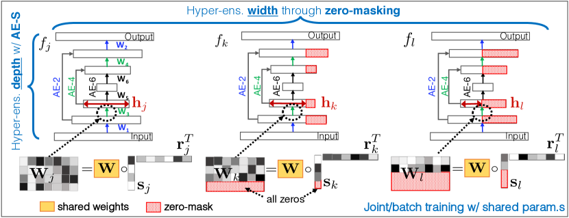
Figure 2: Main design elements in RobOD: (1) AE with Skip links (AE-S): Each AE-S, denoted $f$, hyper-ensembles multiple AE models with various depths (in the figure, AE-2, 4 and 6), with shared parameters; e.g. for $f_{j}$, layer 2 weights $\bm{W}_{j}$ (in dashed circle) is shared among different-depth AEs (i.e. AE-4 and AE-6). (2) Batch ensemble (BE) training with zero-masks: Multiple AE-S models with shared parameters are trained simultaneously, having various widths thanks to zero-masking; e.g. at layer 2, $\bm{W}$ is shared by all three different-width AE-S models in the batch (denoted $f_{j}$, $f_{k}$, $f_{l}$), where hidden sizes follow $|\bm{h}_{j}|>|\bm{h}_{k}|>|\bm{h}_{l}|$ through varying size zero-masks on $\bm{s}_{k}$ and $\bm{s}_{l}$. ($\bm{s}\bm{r}^{T}$ depicts an outer product, and $\circ$ denotes Hadamard/element-wise matrix multiplication.)

4.2 Design Strategies for Speeding up Ensemble Training

4.2.1 Hyper-ensembling depth: One model for multiple depths

Skip or shortcut connections are applied in NNs for various purposes; e.g., in ResNet [21] for solving the depth degradation problem, in JK-Net [45] for representation learning with varying localities, in U-Net [34] and stochastic depth NNs [24] for training models with adaptive depth, and so on.

Due to the “hourglass” structure of the AE, skipping one layer in an AE would cause dimensionality mismatch for the next layer. Instead, we create long shortcuts by skipping the middle layers while keeping the outer encoder-decoder pairs symmetrically, and refer to this architecture as AE-S.

An illustration of hyper-ensembling depth can be found in Fig. 2; see e.g. the AE-S denoted by $f_{j}$. Given a $2L$-layer AE-S ($L$ encoder and $L$ decoder layers), there are $2L$ trainable weight matrices. For input $\mathcal{D}$, we generate $L$ outputs by allowing the input to pass through the outermost encoder-decoder pair (which we denote as $AE\text{-}2$), the two outermost encoder-decoder pairs ($AE\text{-}4$), and so on, until the full structure ($AE\text{-}2L$) is traversed by the input. In effect, this trains $L$ different AEs under one AE-S model. Then, the overall loss $\mathcal{L}_{\text{{\small{\sf AE-S}}}}$ of the depth-hyper-ensembling AE-S is the summation of the member AEs’ reconstruction errors (denoted $\Delta Err$). Eq. (1) gives an example of the loss function for a $6$-layer AE-S as shown in Fig. 2,

AE-S is an implicit hyper-ensemble which allows simultaneous/joint training of AEs with various depths. It is computationally efficient thanks to parameter sharing, as the outer layers’ weights are reused and tuned among different members. Each ensemble member can also play a regularization effect and prevent an AE from producing low scores for outliers due to overfitting. (See Appx. A.4).

4.2.2 Hyper-ensembling width: Zero-masked joint training

BatchEnsemble [42] (BE) is a state-of-the-art parameter-efficient deep ensemble training approach. However, off-the-shelf, it does not allow for hyper-ensebling, that is, all models in the batch are trained with the same HP configuration, and share equal size parameters. Our approach builds on BE, adapting it to simultaneously train varying-width AE-S with shared parameters.

First, we briefly review the BE architecture with $K$ AEs. For a specific layer in BE, weight $\mathbf{W}\in\mathbb{R}^{m\times r}$ is shared across all $K$ individual members, while each member $i$ maintains two trainable rank-1 vectors: $\mathbf{s}_{i}\in\mathbb{R}^{m}$ and $\mathbf{r}_{i}\in\mathbb{R}^{r}$. The outer product ($\cdot$) of $\mathbf{r}_{i}$ and $\mathbf{s}_{i}^{T}$ creates a “mask” (a matrix in $\mathbb{R}^{m\times r}$) onto the shared weight $\mathbf{W}$ and generates individual weight $\overline{\mathbf{W}_{i}}$. For the input mini-batch $\mathbf{X}_{i}\in\mathbb{R}^{n\times m}$, the forward propagation computation is

$$\Phi\big{(}\mathbf{X}_{i}\overline{\mathbf{W}_{i}}\;\big{)}=\Phi\big{(}\mathbf{X}_{i}\;(\mathbf{W}\circ(\mathbf{s}_{i}\cdot\mathbf{r}_{i}^{T}))\big{)}=\Phi\big{(}(\mathbf{X}_{i}\circ\mathbf{s}_{i})\mathbf{W}\circ\mathbf{r}_{i}\big{)}\;,$$ (2)

where $\Phi$ is the activation function, $\circ$ is the element-wise product, and $\mathbf{r}_{i}$ and $\mathbf{s}_{i}$ are broadcasted row-wise or column-wise depending on the shapes at play. To vectorize the calculation for all $K$ members in the ensemble, two matrices $\mathbf{S}\in\mathbb{R}^{K\times m}$ and $\mathbf{R}\in\mathbb{R}^{K\times r}$ are constructed with rows of $\mathbf{s}_{i}$ and $\mathbf{r}_{i}$, respectively. Thus, for the input $\mathbf{X}\in\mathbb{R}^{Km\times n}$, the BE layer computes the next layer as

$$\Phi\big{(}(\mathbf{X}\circ{\mathbf{S}})\mathbf{W}\circ\mathbf{R}\big{)}\;.$$ (3)

Since $\mathbf{X}$ is composed of $K$ mini-batching $\mathbf{X}_{i}$’s tiling up, each member can utilize a different mini-batch of input. The $K$ members are training simultaneously in parallel using one forward pass, thus relieving the memory and computational burden of traditional ensemble methods.

While BE itself is not a hyper-ensemble, we can leverage this architecture to aggregate networks of different widths, also in an efficient way. The widths of a neural network layer correspond to the rows in the weight matrix. For a specific layer, instead of directly operating on $\mathbf{W}$, we instead initialize a zero-one masking vector $\mathbf{\bm{\alpha}}_{i}\in\{0,1\}^{r}$. $\mathbf{\bm{\alpha}}_{i}$ is to element-wise multiply with the $\mathbf{r}_{i}\in\mathbb{R}^{r}$, such that the operation $\mathbf{W}\circ\mathbf{s}_{i}\cdot(\mathbf{r}_{i}^{T}\circ\mathbf{\bm{\alpha}}_{i}^{T})$ will create a masking matrix of size $(m\times r)$ and sparsify the individual weight $\overline{\mathbf{W}_{i}}$ by allowing zero’ed-out rows. In vectorized notation, the matrix $\mathbf{A}\in\{0,1\}^{K\times r}$ is composed of $K$ distinct masking vectors. Then, the zero-masked BE forward propagation becomes

$$\Phi\big{(}\mathbf{X}\circ\mathbf{S})\mathbf{W}\circ(\mathbf{R}\circ\mathbf{A})\big{)}\;.$$ (4)

Sparsifying neural networks has been shown to decrease storage and improve training efficiency, with many algorithms built to wisely prune the neural network [22]. While zero-masked BE is similar to creating neural networks of varying density, our main goal is to obtain models with different widths (i.e. hidden sizes), such that when trained under BE, creates a width-hyper-ensemble. Specifically, we construct the zero-masked BE layer with the maximum width and specify the zeros in respective $\mathbf{\bm{\alpha}}$ vectors, such that the masked-out individual weights correspond to varying-width models.

The zero-masked BE is efficient as $\mathbf{A}$ is fixed throughout training. The element-wise product of the masking incurs little extra time during forward and backward propagation, while all the (rank-1) vectors are cheap to store compared to separate weight matrices as in traditional ensemble training.

4.2.3 RobOD: The overall hyper-ensemble

Let $H$ denote the total number of HPs for an AE-S, where we define a grid of values for each HP; e.g. depth $=$$[4,6,8]$, width $=$$[64,128,256]$, lrn_rate $=$$[1e^{-3},5e^{-4}]$, drop_out $=$$[0.0,0.2]$, etc.

For the two HPs, depth and width, we specify the AE-S with the largest depth value (following Sec. 4.2.1, say $2L$) in the grid and leverage the skip connections to obtain the smaller-depth AEs. Similarly, we specify each AE-S in the zero-masked BE with the largest width value (following Sec. 4.2.2, say $K$) in the grid and leverage the zero-masking to obtain other, smaller-width AEs.

Then, a zero-masked BE trains in parallel $K$ varying-width AE-S models, each being an ensemble of $L$ varying-depth AEs. Outlier score for a point $\mathbf{x}$ is averaged across all $KL$ AE models as

$$s(\mathbf{x})=\frac{1}{KL}\sum_{i=1}^{K}{s_{i}(\mathbf{x})}\;,\;\;\text{where}\;s_{i}(\mathbf{x})=\sum_{d=1}^{L}\lVert\mathbf{x}-f_{i}^{(AE\text{-}2d)}(\mathbf{x};{\bm{\lambda}})\rVert^{2}\;,$$ (5)

where $f_{i}$ is the $i$’th AE-S member, $f_{i}^{(AE\text{-}2d)}$ denotes the AE associated with depth $2d$ within $f_{i}$, and $\bm{\lambda}$ is a vector depicting a specific configuration of all the remaining $(H$$-$$2)$ HPs; e.g. $[$lrn_rate $=$$1e^{-3}$, drop_out $=$$0.2$, etc.$]$. Denoting the total number such configurations by $B$, RobOD averages scores, i.e. the $s(\mathbf{x})$ values, from $B$ different zero-masked BEs as the final outlier score of $\mathbf{x}$.

4.2.4 Further speed up by subsampling

As shown in Eq. 2, BE allows mini-batching, where each data point can be used by one or several different ensemble members. This makes BE a natural fit to subsampling, which further expedites the training procedure. To this end, we create $\{\mathbf{X}_{i}^{in},\mathbf{X}_{i}^{out}\}_{i=1}^{K}$ splits of the training data, where for each AE-S member $i$, we divide the training data into $\mathbf{X}_{i}^{in}$ and $\mathbf{X}_{i}^{out}=\mathbf{X}_{i}/\mathbf{X}_{i}^{in}$ and solely train on mini-batches from $\mathbf{X}_{i}^{in}$. We then compute the out-of-sample outlier score of point $\mathbf{x}$ as $s(\mathbf{x})=\frac{1}{K^{\prime}L}\sum_{i=1}^{K}\mathbbm{1}(\mathbf{x}\in\mathbf{X}_{i}^{out})s_{i}(\mathbf{x})$, where $K^{\prime}=\sum_{i=1}^{K}\mathbbm{1}(\mathbf{x}\in\mathbf{X}_{i}^{out})$.

5 Experiments

5.1 Experimental Setup

Baselines.  We compare to SOTA deep OD methods VanillaAE, RDA [48], DeepSVDD [35] and RandNet [11], the last of which is a deep AE ensemble. We also include the tree-ensemble Isolation Forest [28] (IF) which stands as the SOTA among traditional detectors [12]. Besides RobOD without subsampling, we experiment with two subsampling versions, denoted RobOD-$\delta$, for sampling rates $\delta\in\{0.1,0.5\}$. We also compare to the naïve RobOD with independent training, denoted i-RobOD.

Configurations.  The baselines exhibit 2-8 HPs, per which we define a small grid of values (See Appx. A.5 Table 10). We report the expected AUROC performance, i.e., averaged across all configurations in the grid, along with the standard deviation. For RobOD (and variants) we set $L$$=$$6$, and $K$$=$$8$; the other HP config.s are listed in Appx. Table 11. To measure sensitivity to random initialization, we average performance across 3 runs. All models are trained on a NVIDIA RTX A6000 GPUs server.

Table 3: Dataset statistics.

Name	$\#$ pts.	dim.	outl.$\%$
MNIST-4	6426	1$\times$28$\times$28	10.0
MNIST-5	6426	1$\times$28$\times$28	10.0
MNIST-8	6426	1$\times$28$\times$28	10.0
CIFAR10-0	5500	3$\times$32$\times$32	10.0
CIFAR10-1	5500	3$\times$32$\times$32	10.0
Thyroid	3772	6	2.5
Cardio	1831	21	9.6
Lympho	148	18	4.1

Datasets. We conduct experiments on 5 image datasets from MNIST and CIFAR10, as well as 3 tabular datasets from the ODDS repository. MNIST and CIFAR10 are multi-class, where we pick one class as the inliers and subsample the rest at 10% each to constitute outliers. Datasets have varying outlier % and size, with images having high dimensionality. (See Table 3; MNIST-4, -5, -8 depict respective digits as inliers. CIFAR10-0 and -1 refer to airplane and auto class as inliers, respectively.) Details on dataset description and preparation can be found in Appx. A.5.2. The experiments are all conducted under the Polluted (i.e., transductive) setting.

5.2 Results

With main results shown in Table 4, we want to answer the following questions: Q1. How does RobOD compare to state-of-the-art (SOTA) OD methods? RobOD achieves superior performance to all deep OD baselines on MNIST and tabular datasets, and competitive performance on CIFAR10 datasets against the overall runner-up RandNet. Notably, RobOD performs similarly or even better than i-RobOD, the latter potentially owing to the guarding effect of parameter sharing against overfitting. Moreover, similar performance can be retained under subsampling, where we train each hyper-ensemble member with 50% or even 10% of the data.

Q2. How much does RobOD’s performance vary by initialization? The standard deviation (stdev) of the deep OD baselines is notably large; it is slightly smaller for the ensemble model RandNet, whereas RobOD has significantly smaller stdev, with near-zero sensitivity to random initialization. The sensitivity of deep baselines suggests that with an arbitrary choice of HPs in the absence of any other guidance, one may acquire much less satisfactory outcomes than the average AUROC.

An interesting observation is regarding the traditional IF baseline, which excels on (low-dim.) tabular datasets, and remains competitive on MNIST-4 and CIFAR10-auto. It also shows relatively small variance w.r.t. its (two) HPs. However, it is significantly inferior on other high-dim. image OD tasks, which may be attributed to its lack of representation learning. Nevertheless, the competitiveness of this simple baseline suggests that traditional OD methods cannot be ignored in the ‘horse-race’ of developing new deep OD methods, not only for their competitiveness but also for their robustness to only-a-few HPs that makes them easy to employ by practitioners.

Table 4: AUROC ($\%$) performance of OD methods. Baselines (top) avg.’ed across HP config.s, RobOD and variants (bottom) avg.’ed over 3 runs w/ random init.s.; $\pm$ one stdev. Entries in green depict the method w/ least variance. Highlighted in bold and underline are the best and runner-up.

	MNIST-4	MNIST-5	MNIST-8	CIFAR10-air	CIFAR10-auto	Cardio	Thyroid	Lympho
VanillaAE	81.4$\pm$9.4	73.6$\pm$10.1	83.3$\pm$4.6	60.3$\pm$2.0	59.2$\pm$4.7	87.1$\pm$7.7	81.1 $\pm$8.5	89.4$\pm$11.7
RDA	79.7$\pm$11.2	68.9$\pm$11.4	82.6$\pm$10.2	53.9$\pm$8.8	54.1$\pm$8.9	78.4$\pm$12.1	80.9$\pm$5.3	78.0$\pm$12.2
DeepSVDD	81.9$\pm$4.3	75.7$\pm$3.8	85.3$\pm$3.9	55.6$\pm$3.1	59.0$\pm$3.0	54.6$\pm$7.9	67.5$\pm$15.1	66.5$\pm$15.6
RandNet	85.3$\pm$3.1	79.3$\pm$3.8	85.4$\pm$2.2	59.1$\pm$2.6	59.5$\pm$3.8	89.2$\pm$5.3	81.5$\pm$5.8	92.3$\pm$8.1
IF	84.2$\pm$0.8	70.1$\pm$1.5	70.5$\pm$1.2	42.9$\pm$0.5	62.7$\pm$0.8	94.1$\pm$0.9	97.9$\pm$0.4	99.5$\pm$0.3
RobOD	88.0$\pm$0.0	81.4$\pm$0.1	87.8$\pm$0.0	59.4$\pm$0.0	59.2$\pm$0.1	93.5$\pm$0.1	86.1$\pm$0.6	98.7$\pm$0.1
RobOD-0.5	86.7$\pm$0.1	78.5$\pm$0.1	88.1$\pm$0.1	59.6$\pm$0.5	58.4$\pm$0.3	92.1$\pm$0.3	87.9$\pm$1.3	98.7$\pm$0.1
RobOD-0.1	86.7$\pm$0.0	78.5$\pm$0.1	88.2$\pm$0.1	59.3$\pm$0.0	58.3$\pm$0.2	91.8$\pm$0.3	88.4$\pm$0.5	99.0$\pm$0.1
i-RobOD	84.5$\pm$0.0	74.6$\pm$0.1	87.0$\pm$0.0	62.5$\pm$0.0	61.7$\pm$0.1	87.1$\pm$0.1	93.0$\pm$0.0	98.9$\pm$0.0

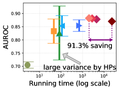
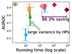
Figure 3: Running time (in log scale) vs. AUROC performance of OD methods (symbols) on (left) MNIST-8 and (right) Cardio. Vertical bars depict one (1) stdev across HP config.s for the baselines.

In Fig. 3 we show the running time (in sec.s) versus the performance for all OD methods (colored symbols) on one image and one tabular dataset for brevity. (See Appx. A.6 Fig. 12 for remaining datasets.) RobOD achieves higher performance, with lower, near-zero variability compared to deep baselines. Traditional IF, based on randomized trees, is very fast, yet it often underperforms on high dimensional tasks such as with images.

Q3. What are the savings in running time compared to naïve hyper-ensemble w/ independent training? We study the savings that RobOD offers compared to the naïve hyper-ensembling. As shown in Table 5, it runs 3-10$\times$ faster across datasets. With subsampling at 10%, RobOD-0.1 runs in about $1.6$-$10$% of what it takes by i-RobOD. Fig. 5 (on MNIST-5) shows that while i-RobOD time increases by the number of models, i.e. larger $L$ and $K$ (fixing other HPs), RobOD takes near-constant time thanks to the batch/simultaneous training of varying-depth and -width members.

Table 5: Running time (sec.) of the naïve ensemble i-RobOD vs. RobOD. RobOD-0.1 that trains with 10% subsampling offers 90-98% relative savings in training time.

	MT-4	MT-5	MT-8	CIF-air	CIF-auto	Cardio	Thy.	Lym.
i-RobOD	24192	24656	23165	38830	39562	8205	14313	1804
RobOD	4521	4630	4456	10721	10722	1070	2049	180
RobOD-0.1	2241	2141	1997	2834	3003	134	295	44
Savings (%)	90.74	91.32	91.38	92.70	92.41	98.37	97.94	97.56

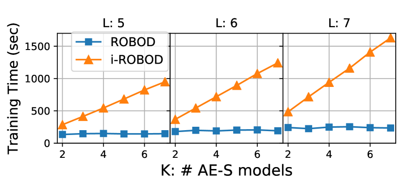
Figure 4: Runtime comparison of RobOD to i-RobOD w/ varying $L$ and $K$.

Q4. How sensitive hyper-ensembles are to their own HPs, which include (1) the selected HP ranges, and (2) the number of sub-models? The two HP terms are directly related, since expanding/shrinking the HP ranges result in more/fewer sub-models constituting the ensemble. We first answer how HP value ranges affect the accuracy of hyper-ensembles. With MNIST-4, we expand, shrink or shift the HP ranges for the VanillaAE, which are consitituents of i-RobOD. The experimental details are provided in Appx. A.7.1. As shown in Table 6, i-RobOD achieves more stable results across all settings. Moreover, i-RobOD produces lower variance with respect to its own HPs than that of the individual model results.

Table 6: Mean and stdev of AUROCs for i-RobOD vs. VanillaAE. i-RobOD’s performance is evaluated with different HP ranges in Table 12. Mean and stdev for VanillaAE are calculated over all constituent sub-models from the same table. The hyper-ensemble i-RobOD has considerably lower performance variation w.r.t. its HPs, than individually traind VanillaAE.

Mean&Std. (i-RobOD)		Mean&Std. (VanillaAE)
83.0$\pm$	2.8	78.9$\pm$	9.8

We also study how number of sub-models impact our model. For the same MNIST-4, DeepSVDD and VanillaAE are selected as the base model for hyper-ensembles, with details in Appx. A.7.2. Fig. 5 shows the AUROC corresponding to different number of sub-models (for DeepSVDD we have both Polluted (left) and Clean (middle) settings, and for VanillaAE we have Polluted (right) setting only). Observe that AUROC quickly stabilizes and the variance shrinks, as the number of sub-models grows beyond a certain size. The larger number of sub-models is, the more stable is the performance.

Finally, we conduct the sensitivity analysis to both HP value ranges and the number of sub-models (since they are correlated) for our proposed RobOD. We evaluate on the Cardio dataset and provide the details in Appx. A.7.3. Table 7 shows that RobOD yields smaller variance to its own HPs and provides more competitive results than other benchmarked models. To summarize, our experiments show that larger number of sub-models and expanded HP ranges under fine grids can relax an hyper-ensemble model’s dependency on its own HPs.

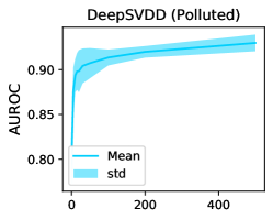
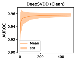
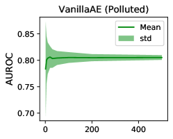
Figure 5: Number of sub-models vs. AUROC of ensembled-OD methods on MNIST-4. Shaded areas depict one (1) stdev around the mean performance of the ensemble. For all cases the performance quickly improves to a stable state after $\sim$20 sub-models, with notably small standard deviation.

Table 7: For Cardio dataset, we provide mean and stdev AUROCs of RobOD and benchmarks from HP ranges in Tables 15 (RobOD) and 10 (benchmarks).The hyper-ensemble RobOD has considerably lower performance variation w.r.t. its HPs.

RobOD		VanillaAE		RDA		DeepSVDD		RandNet		IF
93.6$\pm$	0.4	87.7$\pm$	7.7	78.4$\pm$	12.1	54.6$\pm$	7.9	89.2$\pm$	5.3	94.1$\pm$	0.9

6 Conclusion

In this work, we have provided a thorough analysis on the hyperparameter (HP) sensitivitiy of several state-of-the-art deep outlier detection (OD) methods. Our findings quantitatively confirm that model selection is vital and advocate efforts in this line of research. To this end, we introduce RobOD, a scalable hyper-ensemble OD method that remedies the “choice paralysis” by assembling various autoencoder models of different HP configurations, hence obviating HP/model selection. We speed up ensemble training through novel strategies that simultaneously train varying depth and width models under parameter sharing. Extensive experiments on image and point-cloud datasets show the competitiveness of RobOD compared to existing OD baselines, while providing consistent results across random initializations. We hope that our work increases awareness to the unsupervised model selection challenge for the newly booming deep OD literature and motivates future work on hyperparameter-robust model design.

Checklist

1. For all authors…

   1. Do the main claims made in the abstract and introduction accurately reflect the paper’s contributions and scope? [Yes]

   2. Did you describe the limitations of your work? [Yes] Our solution to tackle hyperparameter (HP) sensitivity for deep OD is an ensemble model. We have emphasized throughout the paper that ensemble training is costlier than training a single model. In fact, one of our key contributions is to speed up ensemble training through novel design strategies, yet, further improvements are left to future research.

   3. Did you discuss any potential negative societal impacts of your work? [N/A]

   4. Have you read the ethics review guidelines and ensured that your paper conforms to them? [Yes]

2. If you are including theoretical results…

   1. Did you state the full set of assumptions of all theoretical results? [N/A]

   2. Did you include complete proofs of all theoretical results? [N/A]

3. If you ran experiments…

   1. Did you include the code, data, and instructions needed to reproduce the main experimental results (either in the supplemental material or as a URL)? [Yes] We open-source our source code (including datasets, our method as well as SOTA methods’ implementations) at https://github.com/xyvivian/ROBOD, to which we point in the Introduction section.

   2. Did you specify all the training details (e.g., data splits, hyperparameters, how they were chosen)? [Yes] Yes. We include the hyperparameters used in sensitivity analysis in Table 1 in Sec. 3. Additional HP information is provided in Appx. A.2.

   3. Did you report error bars (e.g., with respect to the random seed after running experiments multiple times)? [Yes] We report empirical AUROC values across multiple hyperparameter configurations and random initializations and report the mean as well as the standard deviation.

   4. Did you include the total amount of compute and the type of resources used (e.g., type of GPUs, internal cluster, or cloud provider)? [Yes] We report the computational resources in Sec. 5.

4. If you are using existing assets (e.g., code, data, models) or curating/releasing new assets…

   1. If your work uses existing assets, did you cite the creators? [Yes] We utilize standard image datasets (MNIST and CIFAR10) along with 3 tabular dataset. We reference the public repository from which the tabular data are collected.

   2. Did you mention the license of the assets? [No] All the datasets we experimented with are open-source with a public license.

   3. Did you include any new assets either in the supplemental material or as a URL? [No]

   4. Did you discuss whether and how consent was obtained from people whose data you’re using/curating? [N/A]

   5. Did you discuss whether the data you are using/curating contains personally identifiable information or offensive content? [N/A]

5. If you used crowdsourcing or conducted research with human subjects…

   1. Did you include the full text of instructions given to participants and screenshots, if applicable? [N/A]

   2. Did you describe any potential participant risks, with links to Institutional Review Board (IRB) approvals, if applicable? [N/A]

   3. Did you include the estimated hourly wage paid to participants and the total amount spent on participant compensation? [N/A]

Appendix A Appendix

A.1 Preview of Existing Deep OD Methods

Table 8: Representative unsupervised deep OD models from 4 different families (for a broader coverage, see surveys [31, 36, 9]), annotated in terms of data used for training, test, and validation/model selection (if any). No existing work attempts (unsupervised) model selection; vast majority reports results for a fixed (how, unclear) “recommended” config. or tune some but not all HPs using labeled validation and even test (!) data. AE: autoencoder, SSL: self-supervised learning, Clean: inlier-only.

Method	Year	Family	Train	Test	Validation (HP/Model Selection)
RandNet [11]	2017	AE ensemble	Polluted	=Train	None, fixed – sensitivity analysis on some HPs
RDA [48]	2017	AE	Polluted	=Train	Best $\lambda$ on Test, other HPs fixed
DAGMM [49]	2018	AE & density	Clean & Pol.d	Disjoint	None, fixed – sensitivity on reg. param.s $\{\lambda_{1},\lambda_{2}\}$
DeepSVDD [35]	2018	One-Class	Clean	Disjoint	Best $\nu$ on Test, other HPs fixed
DROCC [18]	2020	One-Class	Clean	Disjoint	Validation data to tune some (not all) HPs
HRN [23]	2020	One-Class	Clean	Disjoint	10% of Test for tuning $\{\lambda,n\}$, other HPs fixed
(f-)AnoGAN [37, 38]	2017	GAN	Clean & Pol.d	Disjoint	None, fixed
EGBAD [46]	2018	(Bi)GAN	Clean	Disjoint	None, fixed
GANomaly [4]	2018	GAN	Clean	Disjoint	Best reg. weights $\{w_{adv},w_{con},w_{enc}\}$ on Test, others fixed
GOAD [5]	2020	SSL	Clean	Disjoint	None, fixed
NeuTraL [6]	2020	SSL	Clean	Disjoint	10% of Test for tuning transformation HPs, others fixed

A.2 Details on Hyperparameter-Sensitivity Analysis

Clean versus Polluted Testbed Setup.  For sensitivity analysis, we construct our testbed on several datasets, including MNIST, CIFAR10, Thyroid and Cardio. For MNIST, we choose Digit ‘4’ and ‘5’ as the inlier-class, individually. For CIFAR10, we choose class ‘automobile’ as the inlier-class. The inlier-class is assigned the label 0, while we regard all classes other than the inlier-class as outliers and mark them with label 1 instead. Since MNIST and CIFAR10 are image data, we first apply the global contrast normalization to each individual image. We utilize the default train/test data-split (supported with Pytorch vision package). In the Clean setting, we select only the inlier-class data from train data-split as the training data. We measure and report the AUROC of the compared methods on the test data-split, with label 0 being the inlier-class and 1 being rest of the classes. In the Polluted setting, we utilize all the inlier-class data from the train data-split as the label 0, and we mix the data with $10\%$ outlier-classes’ data within the train data-split.

The tabular data, Thyroid and Cardio, are downloaded from the ODDS repository (available at http://odds.cs.stonybrook.edu/. The data come in Polluted setting, with $2.5\%$ and $9.6\%$ outliers, respectively. The inliers are labeled 0 and outliers are denoted as label 1. For tabular data, we transform and scale each feature between zero and one.

We also conduct experiment using GANomaly [4]’s data (MNIST digit ‘4’ as the outlier class, rest as inliers). The data split and configuration are the same as described in the authors’ provided code.

Model HP Descriptions and Grid of Values. 

• VanillaAE:

  1. n_layers: number of encoder layers (i.e. depth)

  2. layer_decay: the rate of NN width’s shrinkage between current and next encoder layers, the decoder layers are expanded at the same rate.

  3. LR: learning rate

  4. iter: number of epochs/iterations

• RDA:

  1. $\lambda$ (model-specific reg.): a penalty term that tunes the level of sparsity in the outlier matrix $S$ (refer to Section 3.1 in [48]).

  2. n_layers: number of encoder layers (i.e. depth)

  3. layer_decay: the rate of NN width’s shrinkage between current and next encoder layers, the decoder layers are expanded at the same rate.

  4. LR: learning rate

  5. inner_iter: number of epochs/iterations to train the underlying autoencoder (AE), before updating the outlier matrix $S$ and inlier matrix $L$ (refer to Section 4.1 in [48]).

  6. iter: number of epochs/iterations in the algorithm, which first separates the training data into outlier matrix $S$ and inlier matrix $L$, then trains AE on the inlier matrix.

• DeepSVDD:

  1. conv_dim: the output number of channels, after the first- convolutional encoder layer. After the first-layer, the number of channels expand at rate of $2$.

  2. fc_dim: the output dimension of the fully connected layer between convolutional encoder layers and decoder layers, in the LeNet structure [27].

  3. Relu_slope: DeepSVDD utilizes leaky-relu activation to avoid the trivial, uninformative solutions [35]. Here we alter the leakiness of the relu sloping.

  4. pretr_iter: In [35], an AE is pre-trained, to set the hypersphere center $c$ to the mean of the mapped data. pretr_iter determines the number of epochs/iterations to train AE.

  5. pretr_LR: the learning rate to pretrain the AE.

  6. iter: the number of epochs/iterations in training the DeepSVDD

  7. LR: the learning rate during training

  8. wght_dc: weight decay rate

• GANomaly

  1. $w_{adv}$: weight parameter that adjusts the adversarial loss function (See Section 3.2 in [4].)

  2. $w_{con}$: weight parameter that adjusts the contextual loss, for learning the contextual information about the input data (See Section 3.2 in [4].)

  3. $w_{enc}$: weight parameter that adjusts the encoder loss and minimizes the distance between the bottleneck features and the encoder of the generated features (See Section 3.2 in [4].)

  4. z_dim: the dimension of the reduced embedded space after the input is passed through the encoders

  5. LR: learning rate

  6. iter: number of epochs/iterations

• RandNet

  1. n_layers: number of encoder layers (i.e. depth) in BAE

  2. layer_decay: the rate of NN width’s shrinkage between current and next encoder layers, the decoder layers are expanded at the same rate.

  3. sample_r: sample size selection for adaptive sampling (See Section 3.3 in [3].)

  4. ens_size: number of ensemble members/models

  5. pretr_iter: number of epochs/iterations to pretrain the BAE

  6. iter: number of epochs/iterations

  7. LR: learning rate

  8. wght_dc: weight decay rate

Table 9: We define a grid of 1-3 unique values for each hyperparameter (HP) of each deep OD method studied. With 4-to-8 different HPs each, the total number of configurations, and i.e. models trained, quickly grows to several hundreds. When applicable/available, we include the author-recommended value (marked in bold and underlined) in the respective grid.

Method	Hyperparameter	Grid	#values	Method	Hyperparameter	Grid	#values
VanillaAE	n_layers	[2, 3, 4]	3	DeepSVDD	conv_dim	[8, 16, 32]	3
	layer_decay	[1, 2, 4]	3		fc_dim	[16, 32]	2
	LR	[1e-3, 1e-4, 1e-5]	3		Relu_slope	[1e-1, 1e-3]	2
	iter	[200, 500, 1000]	3		pretr_iter	[200, 350, 400]	3
		Total =	81		pretr_LR	[1e-4, 1e-5]	2
RDA	$\lambda$	[5e-1, 5e-3, 5e-5]	3		iter	[100, 200, 250]	3
	n_layers	[2, 3, 4]	3		LR	[1e-4, 1e-5]	2
	layer_decay	[1, 2, 4]	3		wght_dc	[1e-5, 1e-6]	2
	LR	[1e-3, 1e-4]	2			Total #models =	864
	inner_iter	[20, 50]	2	RandNet	n_layers	[3, 5, 7, 9]	4
	iter	[5, 20, 50]	3		layer_decay	[0.3, 0.6]	2
		Total #models =	324		sample_r	[1.00, 1.01]	2
GANomaly	$w_{adv}$	1	1		ens_size	[50, 200]	2
	$w_{con}$	[25, 50, 100]	3		pretr_iter	100	1
	$w_{enc}$	[0.1, 1]	2		iter	[300, 1000]	2
	z_dim	[50, 100, 200]	3		LR	[1e-2, 1e-3, 1e-4]	3
	LR	[5e-3, 2e-3, 5e-4]	3		wght_dc	0	1
	iter	[10, 15, 25]	3			Total #models =	192
		Total #models =	162

A.3 Additional Results: Hyperparameter-Sensitivity Analysis

In Fig. 6, we show the AUROC performance of deep OD methods in Clean setting. In Fig. 7, Fig. 8, Fig. 9 and Fig. 10 we show additional experiment results and AUROC performances over $3$ runs with different random initializations.

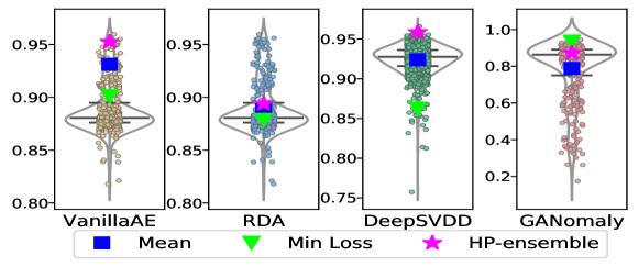
Figure 6: AUROC performance of deep OD methods with different HP configurations (circles) on MNIST-4 with Clean training data showcase notable variation (i.e., sensitivity). Hyper-ensemble (☆) improves notably over Mean ($\square$).

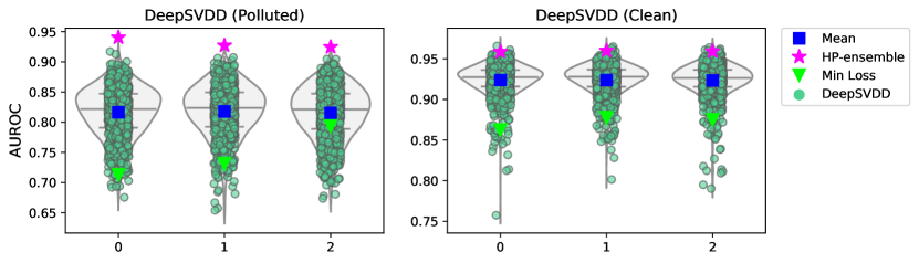
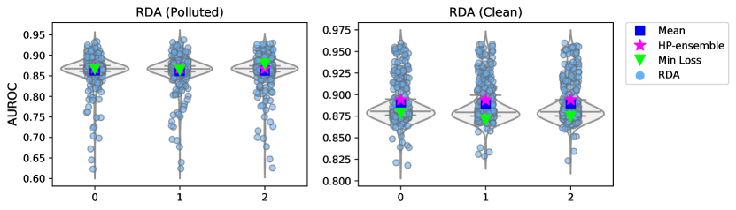
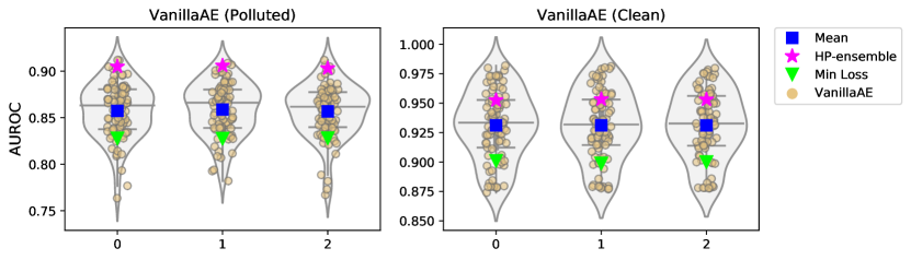
Figure 7: AUROC results under varying HP-configurations on MNIST-4 dataset under the Clean (only train on digit ‘4’ images) and Polluted (digit ‘4’ as inliers, the rest nine classes down-sampled at 10% as outliers) settings. We conduct each experiment 3 times with different random initialization, where each plot’s x-axis corresponds to the experiment index. Note: y-axes are not directly comparable – we use different y-axis to better reflect the spread for each experiment.

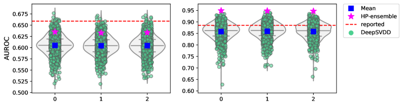
Figure 8: For DeepSVDD algorithm, we show various HP-configurations’ AUROC results under the Clean setting. Left: MNIST digit ‘5’ as the inlier data. Right: CIFAR10 ‘automobile’ as the inlier data. We conduct each experiment 3 times with different random initialization, where each plot’s x-axis corresponds to the experiment index. Performance reported in the original paper [35] appears above what we have obtained on average for both datasets.

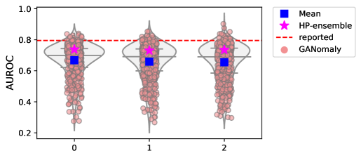
Figure 9: AUROC results with varying HP configurations for the GANomaly algorithm. We utilize the same experimental setting as in [4], with MNIST digit ‘4’ as the outlier class, and rest of the digit classes as inliers (also in Clean setting). The x-axis corresponds to the experiment index among 3 independent runs each with a different random initialization. Performance reported in the original paper [4] appears above what we have obtained on average.

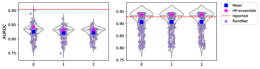
Figure 10: AUROC results with varying HP configurations for the RandNet algorithm. As RandNet implementation contains fully connected layers, we evaluate it only on tabular data under Polluted setting, similar to the experiments in [3]. Left: Thyorid dataset, Right: Cardio dataset. Each plot’s x-axis corresponds to the experiment index for 3 different runs with random initialization.

A.4 Regularization Effect of Weight Sharing

One noticeable problem with applying autoencoders (AE) and reconstruction loss for outlier detection is that for AE, the decision boundary is hard to draw due to noise and outliers that can impact the quality of the reconstruction. In some cases, the AE can overfit to all the data points including the outliers, causing large false negative rate. In other cases, it may underfit to data and fail to reconstruct the input satisfactorily. While the “denoising AEs” [44] or “correntropy AEs” [32] may help to alleviate such problems, they both rely on clean inlier-only data, which is typically not available in real-world scenarios. On the other hand, RobOD with AE-S allows an implicit ensemble of various NN depths and widths and plays a regularization effect on the outliers scores, in effect helping prevent AE from potential failures due to underfitting or overfitting.

To demonstrate the regularization effect with AE-S, we compare the reconstructed images of AE versus AE-S, with number of layers $\{2,4,6,8,10,12,14\}$, respectively (hidden dimension decays at a constant rate of $2$). We compare the individual AE and AE-S, keeping the other HP-configurations same, and training under the Polluted setting with MNIST digit ‘5’ as the inlier class. Fig. 11 shows the reconstructed images with these $7$ individual AEs and a single AE-S ensemble, with implicit AE-i ($i\in\{2\ldots 14\}$). We see that individual AEs are overfitting to the outlier classes (digit ‘3’ and ‘7’) providing good reconstructions when layers $L$ equal to $2$ and $4$. In contrast, they underfit and fail to reconstruct any inliers or outliers when layers $L$ equals to $6$, $8$, and $10$. When $L$ increases to $12$ and $14$ layers, individual AEs provide low-quality reconstructions to both inliers and outliers, distorting all outliers to inlier class (digit ‘5’). In contrast, AE-S provides lower-resolution reconstruction for outlier classes during AE-2 and AE-4, that is overfitting showcases at a lower degree. AE-S can still provide signal to distinguish the outliers from the inliers from AE-6 through AE-12 where the outliers gradually become more blurred and start to deform into inlier’s shape. Only at very large depth at AE-14, AE-S cannot distinguish between outlier instances from inlier instances, providing low quality predictions to both classes.

Intuitively, this regularization effect is due to the weight sharing between AE-i’s. Since the next AE-i utilizes the weights optimized by the previous AE-i, the training phase becomes easier and underfitting is less likely to occur. Moreover, AE-S has a similar structure as U-Net [34], which is known to reduce the overfitting in medical image segmentation tasks.

While both i-RobOD and RobOD average the reconstruction loss from ensemble members, RobOD with AE-S structure (and hence parameter sharing) is able to better capture the outlier information thanks to this regularization effect. This phenomenon also explains why RobOD’s performance is better than that of i-RobOD, e.g. on MNIST datasets in Table 4.

A.5 Details on Experiment Setup

A.5.1 Hyperparameter Configurations: Details

In experiments, we compare to VanillaAE, RDA [48], DeepSVDD [35] and RandNet [11]. We have not compared to GANomaly due to the higher variance of performances we observed during sensitivity analysis. We define a small grid of values for the HPs of each of these methods.

Because DeepSVDD is originally trained with LeNet [27] (Convolutional AE) structure, we also implement Convolutional AEs for algorithms that are either pretrained with AEs, or utilize AEs as the backbone algorithm. The detailed HP configurations are shown in Table 10. The VanillaAE and RandNet are trained with AE for all three kinds of datasets; DeepSVDD is trained with Convolutional AE (LeNet) on image data and AE on tabular data; RDA is trained on AE for MNIST and tabular data, it utilizes Convolutional AE (LeNet) on CIFAR10. If an algorithm is trained with AE as the underlying structure, we define a shared grid of HPs: number of encoder layers, decay rate (the rate of NN width’s shrinkage between current and next encoder layers), dropout rate, train learning rate, etc. Similarly for Convolutional AE, the algorithms apply the same grid of HPs: convolution channels, fully-connected layer dimensions, weight decay, learning rate, etc.

With respect to model-specific HPs, RDA uses $\lambda$ as a penalty constant for sparsity of the outlier matrix. It also uses inner_iters and iter, to specify the number of epochs respectively for training an AE and for separating the data into outlier and inlier matrices. For RandNet, we fix the number of ensemble members to $5$ due to computational overhead in training high-dimensional image datasets, while [3] uses $50$ ensemble members as RandNet is trained on tabular data only. Other model-specific HP descriptions can be found in Sec. A.2 Model HP Descriptions and Grid of Values.

For each data point, i-RobOD provides a score by averaging each individual VanillaAE’s reconstruction error for a data point, thus the training time required for i-RobOD sums up each VanillaAE’s time. RobOD speeds up i-RobOD with fast ensembles across varying NN depths and widths. Table 11 shows the architecture overview for RobOD. Specifically, the NN depths and widths are set to $8$ and $6$, representing the implicit ensembles. RobOD explicitly ensembles over various train iterations, learning rates, dropout rate, weight decay, providing an averaged reconstruction error score for each data point. We also experiment with two subsampling based versions, denoted RobOD-$\delta$, where $\delta=0.1$ and $0.5$, respectively. We let RobOD-$\delta$ to train each ensemble member only on $10\%$ or $50\%$ of the training data, and score “out-of-sample” points, i.e. the rest of the (unseen) data points.

Table 10: Grid of values for the HPs and neural architectures used in experiments.

HPs	AE	LeNet (MNIST)	LeNet (CIFAR10)
Number of encoder layers	[2,3,4,5,6]	[2]	[3]
Decay rate	[1.5,1.75,2,2.25,2.5,2.75,3,3.25]	-	-
Convolution channels	-	[8]	[16]
FC layer dimensions	-	[16,32,64]	[32,64,128]
Dropout rate	[0.0,0.2]	-	-
Weight decay	[0,1e-5]	[0,1e-5,1e-6]	[0,1e-5,1e-6]
Train Learning Rate	[1e-3,1e-4]	[1e-4,1e-5]	[1e-4,1e-5]

NN settings for dataset:	MNIST	CIFAR10	Tabular Data
VanillaAE	AE	AE	AE
DeepSVDD	LeNet (MNIST)	LeNet (CIFAR10)	AE
RDA	AE	LeNet (CIFAR10)	AE
RandNet	AE	AE	AE

Method	Other HP settings
VanillaAE	train iters: [250,500]
RDA	$\lambda$: [1e-1,1e-3,1e-5], iters: [20,30], inner iters: [20,30]
DeepSVDD	LeakyRelu Slope: [1e-1, 1e-3], pretrain iters: [100,350],
	pretrain lr: [1e-4], train iters: [250,500]]
RandNet	pretrain iters: [100], pretrain lr:[1e-4] adaptive sampling rate: [1.0]
	train iters: [250,500], ens_size = [5]

Table 11: RobOD architecture overview

List of HPs	Settings
BatchEnsemble num_models	8 (implicit ensemble over decay rate: [1.5,1.75,2,2.25,2.5,2.75,3,3.25])
num_layers	6 (implicit ensemble over AE-2, AE-4, AE-6,AE-8,AE-10,AE-12)
Train iterations	[250,500]
Train Learning Rate	[1e-3,1e-4]
Dropout rate	[0.0, 0.2]
Weight decay	[0, 1e-5]

A.5.2 Dataset Description

Similar to the experiment settings in our sensitivity analysis, we evaluate the baseline methods and RobOD on image data (MNIST, CIFAR10) as well as tabular data (Thyroid, Cardio and Lympho). For MNIST, we conduct three sets of experiments; each chooses digit ‘4’,‘5’, or ‘8’ as the inlier class, respectively. For CIFAR10, we conduct two sets of experiments, with ‘airplane’ (CIFAR10-0) and ‘automobile’ (CIFAR10-1) as the inlier classes. For image data, we employ global contrast normalization to individual images. The inliers are assigned the label 0 and all classes other than the inlier class will be marked with 1, indicating the outlier class. We conduct all experiments under the Polluted setting, where we use all the inlier class points from Pytorch’s train data-split as label 0, and combine them with $10\%$ of points from the outlier classes within the train data-split. The tabular data, Thyroid, Cardio and Lympho, are downloaded from the ODDS repository (available at http://odds.cs.stonybrook.edu/, which contain $2.5\%$, $9.6\%$ and $4.1\%$ outliers, respectively. Similar to image data, the inliers have label 0 and outliers have label 1. Prior to model training, we transform and scale each feature between zero and one using the MinMaxScaler.

A.6 Additional Experiment Results

Fig. 11 is shown to illustrate the regularization effect of parameter sharing in AE-S versus a vanilla AE. (See A.4 for discussion.)

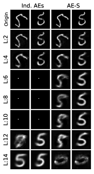
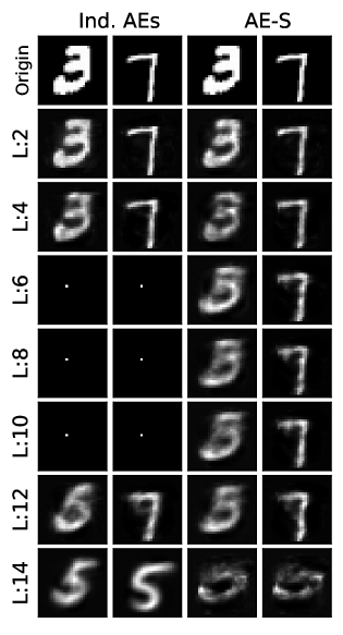
Figure 11: Left: Reconstructed inlier class instances (MNIST digit ‘5’), generated by individual AEs vs AE-S structure in RobOD. Right: Reconstructed outlier class instances (MNIST digit ‘3’ and ‘7’) by individual AEs versus AE-S structure. L denotes the number of layers.

Fig. 12 shows the running time (in log scale) vs. AUROC performance of OD methods (symbols) on datasets MNIST-4, MNIST-5, CIFAR-airplane, CIFAR-automobile, Thyroid and Lympho.

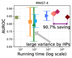
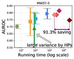
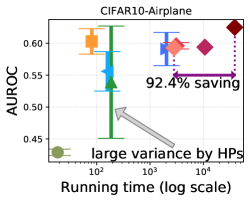
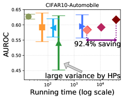
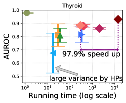
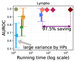
Figure 12: Running time (in log scale) vs. AUROC of OD methods (symbols) on other datasets. Vertical bars depict one (1) stdev across HP config.s. RobOD often improves detection performance and importantly, provides robust low-variance performance. Sampling based RobOD reduces running time considerably with small difference in relative performance.

A.7 HP Sensitivity Analysis for Ensemble Models

In this section, we want to show whether or not hyper-ensembles are robust to their own HPs: (1) the HP value ranges, and (2) the number of sub-models. We remark that the number of sub-models and HP ranges are directly related for a hyper-ensemble, since expanding (or shrinking) the HP ranges result in more (or fewer) sub-models constituting the ensemble. Finally, we show how the proposed RobOD is robust to both the number of sub-models and varying HP value ranges.

A.7.1 How do HP value ranges affect the ensemble?

Starting with the same HP settings as in Table 10 for VanillaAE, we expand, shrink or shift the HP ranges for the VanillaAE models, and then measure the resulting accuracy and variance of i-RobOD, which assembles multiple VanillaAEs. Table 12 summarizes the various actions taken as compared to the original settings. For example, in Row 1, the range for the number of auto-encoders is expanded to also include $[7,8,9]$ layers, or shifted to exhibit auto-encoders with $[6,7,8,9]$ layers, shifting from original $[2,3,4,5,6]$ layers. Other HPs are also altered in a similar fashion.

Table 12: Overview of i-RobOD with several HP ranges

List of HPs	Original Setting	Actions
Number of encoder layers	[2,3,4,5,6]	Expand:[2,3,4,5,6,7,8,9], Shift:[6,7,8,9], Shrink:[2,3,4]
Train iterations	[250,500]	Shift&Shrink:[1000], Expand:[250,500,1000]
Decay rate	[1.5-3.25]	Shrink:[1.5-2.0]
Train Learning Rate	[1e-3,1e-4]	Shift:[1e-2,1e-3], Expand:[1e-2,1e-3,1e-4]
Dropout rate	[0.0, 0.2]	Shift:[0.2,0.5], Expand:[0.0,0.2,0.5]
Weight decay	[0.0, 1e-5]	Shift: [1e-3,1e-4], Expand: [1e-3,1e-4,1e-5,0.0]

We conduct our experiments on the same MNIST dataset with ‘4’ being the inlier digit. For each experiment, we alter a subset of the HPs from Table 12 and record the AUROC across $3$ runs. We measure the mean and standard deviation of i-RobOD AUROC in comparison with VanillaAE’s. Table 6 provides the mean and variance of i-RobOD, evaluated on the performances over all these experimental runs, in comparison to training individual VanillaAE. (Detailed results are in Table 13.)

Our results shows that i-RobOD produces more stable results in all settings than individually trained models. Moreover, it produces lower variance with respect to its own HPs ($2.8$) than that of the individual model results ($9.8$). Because of the lack of any prior knowledge, for many new models and architectures, finding a “good” HP range (a set of HPs that potentially contain the best HP for the task) can be hard. In that case, both the hyper-ensemble and an individual model may achieve less than satisfactory performance. However, hyper-ensemble is likely to achieve better stability to the range of HPs, while individual models are more sensitive when finding the optimal range is unreachable due to lack of validation.

Table 13: The altered HP ranges and AUROC results for i-RobOD and VanillaAE. For example, “Number of encoder layers:[6,7,8,9]” means the values are shifted from [2,3,4,5,6] in the original experiment settings to [6,7,8,9], while the other HPs are the same as before as shown in Table 12.

Altered HP Ranges	Mean&Std. (i-RobOD)		Mean&Std. (VanillaAE)
No Changes	84.5$\pm$	0.0	81.4$\pm$	9.4
Number of encoder layer: [2,3,4]	86.1$\pm$	0.0	85.1$\pm$	6.0
Number of encoder layer:[6,7,8,9]	77.4$\pm$	0.1	75.1$\pm$	7.1
Number of encoder layer: [2,3,4,5,6,7,8,9]	82.1$\pm$	0.0	79.6$\pm$	8.9
Train learning rate: [1e-2,1e-3]	83.3$\pm$	0.2	79.7$\pm$	12.5
Train learning rate: [1e-2,1e-3,1e-4]	83.2$\pm$	0.1	79.4$\pm$	12.3
Dropout rate: [0.2,0.5]	83.6$\pm$	0.2	80.7$\pm$	9.5
Dropout rate: [0.0,0.2,0.5]	84.1$\pm$	0.1	81.1$\pm$	9.6
Train iterations:[1000]	84.5$\pm$	0.2	80.1$\pm$	9.6
Train iterations:[250,500,1000]	84.5$\pm$	0.1	81.2$\pm$	9.0
Weight decay: [1e-3,1e-4]	79.4$\pm$	0.1	77.9$\pm$	3.8
Weight decay: [1e-3,1e-4,1e-5,0.0]	82.6$\pm$	0.1	80.2$\pm$	8.2
Decay rate: [1.5,1.75,2.0]	81.4$\pm$	0.1	78.6$\pm$	13.4

A.7.2 How does the number of sub-models affect the ensemble?

Next we investigate how the number of sub-models change the performance of various deep ensemble models. Here, we choose DeepSVDD and VanillaAE as the baseline ensembles, for which results under 764 and 6,912 individual models are reported in Table 14, conducted on MNIST-4 dataset. We subsample the sub-models among all the $764$ and $6,912$ models, with sizes equal to $[1,5,10,15,20,30,50,100,200,500]$. We conduct each subsampling $100$ times independently, and since we have $3$ experimental runs reported in the previous sections of the paper, we provide the results regarding detection accuracy and variances among $3\times 100$ experimental runs.

Table 14: We define a grid of values for each HP of our studied DeepSVDD and VanillaAE. With 4-to-8 different HPs each, the total number of configurations quickly grows to several hundreds.

Method	Hyperparameter	Grid	#values	Method	Hyperparameter	Grid	#values
VanillaAE	n_layers	[2,3,4,5, 6,7,8,9]	8	DeepSVDD	conv_dim	[8, 16, 32]	3
	layer_decay	[1.5,1.75,2,2.25,2.5,2.75,3,3.25]	8		fc_dim	[16, 32]	2
	LR	[1e-2, 1e-3, 1e-4]	3		Relu_slope	[1e-1, 1e-3]	2
	iter	[200, 500, 1000]	3		pretr_iter	[200, 350, 400]	3
	wght_dc	[1e-3,1e-4,1e-5,0]	4		pretr_LR	[1e-4, 1e-5]	2
	Dropout	[0.0, 0.2, 0.5]	3		iter	[100, 200, 250]	3
		Total #models =	6,912		LR	[1e-4, 1e-5]	2
					wght_dc	[1e-5, 1e-6]	2
						Total #models =	864

Fig. 5 shows the AUROC corresponding to different number of sub-models (for DeepSVDD we have both Polluted (left) and Clean (middle) settings, and for VanillaAE we have Polluted (right) setting only). Notice that when the number of sub-models is less than 20, the overall performance variance is relatively larger, where the ensemble performance is similar to an individual model prediction. AUROC quickly stabilizes and the variance shrinks as the number of sub-models becomes larger than 20 –especially for the DeepSVDD’s Clean setting and VanillaAE’s Polluted setting– with little difference beyond. These results suggest that ensembles are not sensitive to the number of sub-models beyond a certain size, where the larger the number, the more stable is the performance.

A.7.3 HP Sensitivity Analysis: RobOD

In this section, we perform the sensitivity analysis to both HP value ranges as well as the number of sub-models (since they are correlated) for our proposed RobOD. We extend, shrink or shift the number of layers and number of BatchEnsemble models within the AE-S structure, which corresponds to changing the HP-ranges of NN widths and depths. We also recognize the additional training HPs such as train iterations, learning rate, dropout rate, weight decay, etc. Table 15 summarizes the HP-ranges we used to conduct our HP-sensitivity analysis based on Table 11. These additional experiments are on the Cardio dataset. For each set of HP configurations, we repeat $3$ experimental runs and summarizes mean and variance of RobOD’s AUROC. The results among different hyper-ensembles (for both HP ranges and number of sub-models) are given in the following two tables, Table 16 (which alters the AE-S structure HPs) and Table 17 (which alters the other training HPs).

Our results on RobOD match with the two observations in the previous subsections, in that RobOD, the sped-up version of the i-RobOD hyper-ensemble, provides stable results with the varying (1) number of sub-models, and (2) HP value ranges. Moreover, the mean performance and standard deviation of all RobOD experiments listed in Tables 16 and 17 are considerably more competitive than all the other benchmarked models we studied, while RobOD yields smaller variance to its own HP configurations than many banchmarked models (Table 7).

Our analyses provide practical insights on how to reduce an ensemble model’s sensitivity to their HP settings. As long as time and resources permit, one should employ as many number of sub-models as possible, and expand the HP value ranges under a fine grid. In contrast, finding a single set of optimal/good HPs for an individual OD model is almost infeasible for the unsupervised setting.

Table 15: RobOD HP-ranges overview. Note that num_models corresponds to implicit ensemble over decay rate [1.5,1.75,2,2.25,2.5,2.75,3,3.25] (see Table 11), and num_layers corresponds to implicit ensemble over AE-i; e.g. num_layers=6 assembles over AE-2, AE-4, AE-6, AE-8, AE-10, and AE-12.

List of HPs	Original Settings	Actions
BatchEnsemble num_models	8	Shrink:[4] Shrink:[5] Shrink:[6] Shrink:[7]
num_layers	6	Shrink:[4] Expand:[8]
Train iterations	[250,500]	Shift:[500,1000] Expand:[250,500,1000] Shrink: [250]
Train Learning Rate	[1e-3,1e-4]	Shift:[1e-1,1e-2] Expand: [1e-1,1e-2,1e-3,1e-4]
Dropout rate	[0.0, 0.2]	Shrink&Shift:[0.5] Expand: [0.0,0.2,0.5]
Weight decay	[0, 1e-5]	Expand: [1e-4,1e-5,0] Shrink: [0]

Table 16: Results of RobOD over different AE-S structures. With different num_models and num_layers, various number of AE models are implicitly assembled. We report the mean AUROC and standard deviation across $3$ runs, along with the number of (implicit) sub-models in parenthesis.

Mean&Std. for different AE-S structures and the number of sub-models
	num_models:4	num_models:5	num_models:6	num_models:7
num_layers:4	92.4$\pm$0.6 (128)	93.3$\pm$0.3 (160)	93.1$\pm$0.4 (192)	93.3$\pm$0.2 (224)
num_layers:6	93.6$\pm$0.4 (192)	93.6$\pm$0.1 (240)	93.5$\pm$0.1 (288)	93.8$\pm$0.3 (336)
num_layers:8	93.8$\pm$0.1 (256)	93.7$\pm$0.1 (320)	93.5$\pm$0.1 (384)	93.8$\pm$0.1 (448)

Table 17: The altered HPs and results for RobOD. For example, “Train iterations: [250,500,1000]” means that the training iterations are expanded from the original experiment settings (see Table 15) to include the additional value [1000], while the AE-S HPs are the same as before (BatchEnsemble num_models equals to 8, num_layers equals to 6). Mean and Std. of AUROC over 3 runs are reported.

Altered HP Ranges	Mean&Std. (RobOD)
No Changes (384 submodels)	93.5$\pm$	0.1
Train iterations: [250,500,1000] (576 submodels)	93.7$\pm$	0.1
Train iterations: [250] (191 submodels)	94.0$\pm$	0.2
Train Learning Rate: [1e-1,1e-2] (384 submodels)	93.7$\pm$	0.2
Train Learning Rate: [1e-1,1e-2,1e-3,1e-4] (576 submodels)	93.8$\pm$	0.0
Dropout Rate: [0.5] (191 submodels)	93.7$\pm$	0.1
Dropout Rate: [0.0,0.2,0.5] (576 submodels)	93.6$\pm$	0.2
Weight Decay: [1e-4,1e-5,0.0] (576 submodels)	94.0$\pm$	0.0
Weight Decay: [0.0] (191 submodels)	93.7$\pm$	0.3

References

- Aggarwal [2016] C. C. Aggarwal. Outlier Analysis. Springer Publishing Company, Incorporated, 2nd edition, 2016. ISBN 3319475770.
- Aggarwal and Sathe [2015] C. C. Aggarwal and S. Sathe. Theoretical foundations and algorithms for outlier ensembles. SIGKDD Explor., 17(1):24–47, 2015.
- Aggarwal and Sathe [2017] C. C. Aggarwal and S. Sathe. Outlier ensembles: An introduction. Springer, 2017.
- Akcay et al. [2018] S. Akcay, A. Atapour-Abarghouei, and T. P. Breckon. Ganomaly: Semi-supervised anomaly detection via adversarial training. In Asian conference on computer vision, pages 622–637. Springer, 2018.
- Bergman and Hoshen [2020] L. Bergman and Y. Hoshen. Classification-based anomaly detection for general data. In ICLR, 2020. URL https://openreview.net/forum?id=H1lK_lBtvS.
- Boyd et al. [2020] A. Boyd, R. Bamler, S. Mandt, and P. Smyth. Neural transformation learning for deep anomaly detection beyond images. In 34th Conference on Neural Information Processing Systems, 2020.
- Breunig et al. [2000] M. M. Breunig, H.-P. Kriegel, R. T. Ng, and J. Sander. LOF: Identifying density-based local outliers. In SIGMOD Conference, pages 93–104. ACM, 2000. URL http://dblp.uni-trier.de/db/conf/sigmod/sigmod2000.html#BreunigKNS00. SIGMOD Record 29(2), June 2000.
- Campos et al. [2016] G. O. Campos, A. Zimek, J. Sander, R. J. G. B. Campello, B. Micenková, E. Schubert, I. Assent, and M. E. Houle. On the evaluation of unsupervised outlier detection: measures, datasets, and an empirical study. Data Min. Knowl. Discov., 30(4):891–927, 2016. doi: 10.1007/s10618-015-0444-8. URL https://doi.org/10.1007/s10618-015-0444-8.
- Chalapathy and Chawla [2019] R. Chalapathy and S. Chawla. Deep learning for anomaly detection: A survey, 2019. URL http://arxiv.org/abs/1901.03407. cite arxiv:1901.03407.
- Chandola et al. [2009] V. Chandola, A. Banerjee, and V. Kumar. Anomaly detection: A survey. ACM Computing Surveys, 41(3):15:1–15:58, July 2009. ISSN 0360-0300. doi: 10.1145/1541880.1541882. URL http://doi.acm.org/10.1145/1541880.1541882.
- Chen et al. [2017] J. Chen, S. Sathe, C. C. Aggarwal, and D. S. Turaga. Outlier detection with autoencoder ensembles. In N. V. Chawla and W. Wang, editors, SDM, pages 90–98. SIAM, 2017. ISBN 978-1-61197-497-3. URL http://dblp.uni-trier.de/db/conf/sdm/sdm2017.html#ChenSAT17.
- Emmott et al. [2015] A. Emmott, S. Das, T. Dietterich, A. Fern, and W.-K. Wong. A meta-analysis of the anomaly detection problem. arXiv preprint arXiv:1503.01158, 2015.
- Ghafoori and Leckie [2020] Z. Ghafoori and C. Leckie. Deep multi-sphere support vector data description. In SDM, pages 109–117. SIAM, 2020.
- Ghafoori et al. [2018] Z. Ghafoori, S. M. Erfani, S. Rajasegarar, J. C. Bezdek, S. Karunasekera, and C. Leckie. Efficient unsupervised parameter estimation for one-class support vector machines. IEEE transactions on neural networks and learning systems, 29(10):5057–5070, 2018.
- Goix [2016] N. Goix. How to evaluate the quality of unsupervised anomaly detection algorithms? CoRR, abs/1607.01152, 2016. URL http://dblp.uni-trier.de/db/journals/corr/corr1607.html#Goix16.
- Golan and El-Yaniv [2018] I. Golan and R. El-Yaniv. Deep anomaly detection using geometric transformations. In S. Bengio, H. M. Wallach, H. Larochelle, K. Grauman, N. Cesa-Bianchi, and R. Garnett, editors, NeurIPS, pages 9781–9791, 2018. URL http://dblp.uni-trier.de/db/conf/nips/nips2018.html#GolanE18.
- Goldstein and Uchida [2016] M. Goldstein and S. Uchida. A comparative evaluation of unsupervised anomaly detection algorithms for multivariate data. PLOS, 11(4), 2016.
- Goyal et al. [2020] S. Goyal, A. Raghunathan, M. Jain, H. V. Simhadri, and P. Jain. Drocc: Deep robust one-class classification. In International Conference on Machine Learning, pages 3711–3721. PMLR, 2020.
- Guan et al. [2020] H. Guan, L. K. Mokadam, X. Shen, S.-H. Lim, and R. M. Patton. Fleet: Flexible efficient ensemble training for heterogeneous deep neural networks. In I. S. Dhillon, D. S. Papailiopoulos, and V. Sze, editors, MLSys. mlsys.org, 2020. URL http://dblp.uni-trier.de/db/conf/mlsys/mlsys2020.html#GuanMSLP20.
- Guo et al. [2017] C. Guo, G. Pleiss, Y. Sun, and K. Q. Weinberger. On calibration of modern neural networks. In International Conference on Machine Learning, pages 1321–1330, 2017.
- He et al. [2016] K. He, X. Zhang, S. Ren, and J. Sun. Deep residual learning for image recognition. In CVPR, pages 770–778. IEEE Computer Society, 2016. ISBN 978-1-4673-8851-1. URL http://dblp.uni-trier.de/db/conf/cvpr/cvpr2016.html#HeZRS16.
- Hoefler et al. [2021] T. Hoefler, D. Alistarh, T. Ben-Nun, N. Dryden, and A. Peste. Sparsity in deep learning: Pruning and growth for efficient inference and training in neural networks. Journal of Machine Learning Research, 22(241):1–124, 2021.
- Hu et al. [2020] W. Hu, M. Wang, Q. Qin, J. Ma, and B. Liu. Hrn: A holistic approach to one class learning. Advances in Neural Information Processing Systems, 33:19111–19124, 2020.
- Huang et al. [2016] G. Huang, Y. Sun, Z. Liu, D. Sedra, and K. Q. Weinberger. Deep networks with stochastic depth. In B. Leibe, J. Matas, N. Sebe, and M. Welling, editors, ECCV (4), volume 9908 of Lecture Notes in Computer Science, pages 646–661. Springer, 2016. ISBN 978-3-319-46492-3. URL http://dblp.uni-trier.de/db/conf/eccv/eccv2016-4.html#HuangSLSW16.
- Lakshminarayanan et al. [2017] B. Lakshminarayanan, A. Pritzel, and C. Blundell. Simple and scalable predictive uncertainty estimation using deep ensembles. In I. Guyon, U. von Luxburg, S. Bengio, H. M. Wallach, R. Fergus, S. V. N. Vishwanathan, and R. Garnett, editors, NIPS, pages 6402–6413, 2017. URL http://dblp.uni-trier.de/db/conf/nips/nips2017.html#Lakshminarayanan17.
- Lazarevic and Kumar [2005] A. Lazarevic and V. Kumar. Feature bagging for outlier detection. In R. Grossman, R. J. Bayardo, and K. P. Bennett, editors, KDD, pages 157–166. ACM, 2005. ISBN 1-59593-135-X. URL http://dblp.uni-trier.de/db/conf/kdd/kdd2005.html#LazarevicK05.
- Lecun et al. [1998] Y. Lecun, L. Bottou, Y. Bengio, and P. Haffner. Gradient-based learning applied to document recognition. Proceedings of the IEEE, 86(11):2278–2324, 1998. doi: 10.1109/5.726791.
- Liu et al. [2008] F. T. Liu, K. M. Ting, and Z.-H. Zhou. Isolation forest. In ICDM, pages 413–422. IEEE Computer Society, 2008. ISBN 978-0-7695-3502-9. URL http://dblp.uni-trier.de/db/conf/icdm/icdm2008.html#LiuTZ08.
- Marques et al. [2015] H. O. Marques, R. J. G. B. Campello, A. Zimek, and J. Sander. On the internal evaluation of unsupervised outlier detection. In SSDBM, pages 7:1–7:12. ACM, 2015. URL http://dblp.uni-trier.de/db/conf/ssdbm/ssdbm2015.html#MarquesCZS15.
- Nguyen et al. [2017] V. Nguyen, T. Nguyen, and U. Nguyen. An evaluation method for unsupervised anomaly detection algorithms. Journal of Computer Science and Cybernetics, 32(3):259–272, 2017. ISSN 1813-9663. doi: 10.15625/1813-9663/32/3/8455. URL http://vjs.ac.vn/index.php/jcc/article/view/8455.
- Pang et al. [2021] G. Pang, C. Shen, L. Cao, and A. V. D. Hengel. Deep learning for anomaly detection: A review. ACM Computing Surveys (CSUR), 54(2):1–38, 2021.
- Qi et al. [2014] Y. Qi, Y. Wang, X. Zheng, and Z. Wu. Robust feature learning by stacked autoencoder with maximum correntropy criterion. In 2014 IEEE International Conference on Acoustics, Speech and Signal Processing (ICASSP), pages 6716–6720, 2014. doi: 10.1109/ICASSP.2014.6854900.
- Rayana and Akoglu [2016] S. Rayana and L. Akoglu. Less is more: Building selective anomaly ensembles. ACM Trans. Knowl. Discov. Data, 10(4):42:1–42:33, 2016. URL http://dblp.uni-trier.de/db/journals/tkdd/tkdd10.html#RayanaA16.
- Ronneberger et al. [2015] O. Ronneberger, P. Fischer, and T. Brox. U-net: Convolutional networks for biomedical image segmentation. In N. Navab, J. Hornegger, W. M. Wells, and A. F. Frangi, editors, Medical Image Computing and Computer-Assisted Intervention – MICCAI 2015, pages 234–241, Cham, 2015. Springer International Publishing. ISBN 978-3-319-24574-4.
- Ruff et al. [2018] L. Ruff, N. Görnitz, L. Deecke, S. A. Siddiqui, R. A. Vandermeulen, A. Binder, E. Müller, and M. Kloft. Deep one-class classification. In J. G. Dy and A. Krause, editors, ICML, volume 80, pages 4390–4399. PMLR, 2018. URL http://proceedings.mlr.press/v80/ruff18a/ruff18a.pdf.
- Ruff et al. [2021] L. Ruff, J. R. Kauffmann, R. A. Vandermeulen, G. Montavon, W. Samek, M. Kloft, T. G. Dietterich, and K.-R. Müller. A unifying review of deep and shallow anomaly detection. Proceedings of the IEEE, 109(5):756–795, May 2021. ISSN 1558-2256. doi: 10.1109/JPROC.2021.3052449.
- Schlegl et al. [2017] T. Schlegl, P. Seeböck, S. M. Waldstein, U. Schmidt-Erfurth, and G. Langs. Unsupervised anomaly detection with generative adversarial networks to guide marker discovery. In M. Niethammer, M. Styner, S. R. Aylward, H. Zhu, I. Oguz, P.-T. Yap, and D. Shen, editors, IPMI, volume 10265 of Lecture Notes in Computer Science, pages 146–157. Springer, 2017. ISBN 978-3-319-59050-9. URL http://dblp.uni-trier.de/db/conf/ipmi/ipmi2017.html#SchleglSWSL17.
- Schlegl et al. [2019] T. Schlegl, P. Seeböck, S. M. Waldstein, G. Langs, and U. Schmidt-Erfurth. f-anogan: Fast unsupervised anomaly detection with generative adversarial networks. Medical Image Anal., 54:30–44, 2019. URL http://dblp.uni-trier.de/db/journals/mia/mia54.html#SchleglSWLS19.
- Schölkopf et al. [1999] B. Schölkopf, R. C. Williamson, A. J. Smola, J. Shawe-Taylor, and J. C. Platt. Support vector method for novelty detection. In NIPS, pages 582–588. The MIT Press, 1999. URL http://dblp.uni-trier.de/db/conf/nips/nips1999.html#ScholkopfWSSP99.
- Tax and Duin [2001] D. M. Tax and R. P. Duin. Outliers and data descriptions. In Proceedings of the 7th Annual Conference of the Advanced School for Computing and Imaging, pages 234–241, 2001.
- Wang et al. [2018] S. Wang, Q. Liu, E. Zhu, F. Porikli, and J. Yin. Hyperparameter selection of one-class support vector machine by self-adaptive data shifting. Pattern Recognition, 74:198–211, 2018.
- Wen et al. [2020] Y. Wen, D. Tran, and J. Ba. BatchEnsemble: an alternative approach to efficient ensemble and lifelong learning. In ICLR. OpenReview.net, 2020. URL http://dblp.uni-trier.de/db/conf/iclr/iclr2020.html#WenTB20.
- Wenzel et al. [2020] F. Wenzel, J. Snoek, D. Tran, and R. Jenatton. Hyperparameter ensembles for robustness and uncertainty quantification. arXiv preprint arXiv:2006.13570, 2020.
- Xie et al. [2012] J. Xie, L. Xu, and E. Chen. Image denoising and inpainting with deep neural networks. In Proceedings of the 25th International Conference on Neural Information Processing Systems - Volume 1, NIPS’12, page 341–349, Red Hook, NY, USA, 2012. Curran Associates Inc.
- Xu et al. [2018] K. Xu, C. Li, Y. Tian, T. Sonobe, K.-i. Kawarabayashi, and S. Jegelka. Representation Learning on Graphs with Jumping Knowledge Networks. volume 80 of Proceedings of Machine Learning Research, pages 5453–5462, Stockholmsmässan, Stockholm Sweden, 2018. PMLR. URL http://proceedings.mlr.press/v80/xu18c.html.
- Zenati et al. [2018] H. Zenati, C. S. Foo, B. Lecouat, G. Manek, and V. R. Chandrasekhar. Efficient gan-based anomaly detection. arXiv preprint arXiv:1802.06222, 2018.
- Zhao et al. [2021] Y. Zhao, R. Rossi, and L. Akoglu. Automatic unsupervised outlier model selection. In Thirty-Fifth Conference on Neural Information Processing Systems, 2021.
- Zhou and Paffenroth [2017] C. Zhou and R. C. Paffenroth. Anomaly detection with robust deep autoencoders. In KDD, pages 665–674. ACM, 2017. ISBN 978-1-4503-4887-4. URL http://dblp.uni-trier.de/db/conf/kdd/kdd2017.html#ZhouP17.
- Zong et al. [2018] B. Zong, Q. Song, M. R. Min, W. Cheng, C. Lumezanu, D. ki Cho, and H. Chen. Deep autoencoding gaussian mixture model for unsupervised anomaly detection. In ICLR. OpenReview.net, 2018. URL http://dblp.uni-trier.de/db/conf/iclr/iclr2018.html#ZongSMCLCC18.