Convergence and Price of Anarchy Guarantees of the
Softmax Policy Gradient in Markov Potential Games

Abstract

We study the performance of policy gradient methods for the subclass of Markov games known as Markov potential games (MPGs), which extends the notion of normal-form potential games to the stateful setting and includes the important special case of the fully cooperative setting where the agents share an identical reward function. Our focus in this paper is to study the convergence of the policy gradient method for solving MPGs under softmax policy parameterization, both tabular and parameterized with general function approximators such as neural networks. We first show the asymptotic convergence of this method to a Nash equilibrium of MPGs for tabular softmax policies. Second, we derive the finite-time performance of the policy gradient in two settings: 1) using the log-barrier regularization, and 2) using the natural policy gradient under the best-response dynamics (NPG-BR). Finally, extending the notion of price of anarchy (POA) and smoothness in normal-form games, we introduce the POA for MPGs and provide a POA bound for NPG-BR. To our knowledge, this is the first POA bound for solving MPGs. To support our theoretical results, we empirically compare the convergence rates and POA of policy gradient variants for both tabular and neural softmax policies.

1 Introduction

The framework of multi-agent sequential decision making is often formulated as (variants of) Markov games (MGs) (Shapley, 1953), which finds a wide range of real-world applications such as coordination of multi-robot systems (Corke et al., 2005), traffic control (Chu et al., 2019), power grid management (Callaway & Hiskens, 2010), etc. Perhaps the most well-known solution concept for MGs is the Nash policy, which is also known as the Nash equilibrium in the special case of stateless Markov games (i.e., normal-form games). In a Nash policy, every agent selects its actions independently of any other agent given the state and plays a best response to all other agents. In the special case of single-agent Markov games, aka Markov decision processes (MDPs), Nash policies reduce to the agent’s optimal policies. Most existing algorithms seeking to find Nash policies are value-based (i.e., computing only value functions related to the MG), with examples including Nash Q-learning (Hu & Wellman, 2003), Hyper-Q Learning (Tesauro, 2003), and Nash-VI for the special case of zero-sum MGs (Zhang et al., 2020). Policy-based algorithms, including multi-agent actor-critic algorithms, have recently gained attention with impressive empirical success (Lowe et al., 2017; Foerster et al., 2017) as well as provable guarantees (Zhang et al., 2018; Leonardos et al., 2021; Zhang et al., 2021).

This paper focuses on the MG subclass of Markov potential games (MPGs) (Macua et al., 2018; Leonardos et al., 2021; Zhang et al., 2021), which is extended from the notion of (normal-form) potential game and also incorporates as a special case the fully cooperative MGs where all agents share the same reward to optimize. The MPG structure allows for exploiting recent advances in single-agent policy gradient methods (e.g., (Agarwal et al., 2019)) to establish the convergence of policy gradient to (near-)Nash policies in MPGs. Specifically, existing work has established finite-time convergence guarantees under the direct policy parameterization. In this paper, we are interested in the alternative softmax policy parameterization, both tabularly and with neural networks for learnable state representations. For tabular softmax, we establish several convergence guarantees to (near-)Nash policies in MPGs in Section 3, extending their counterpart from the single-agent setting (Agarwal et al., 2019). We then empirically compare tabular softmax with neural network-based softmax parameterization in terms of their convergence rates.

MPGs can model many problems where outcomes of high social welfare, measured by the sum of all agents’ values, are most desirable. In these scenarios, the solution concept of the Nash policy is inadequate. The price of anarchy (POA) of a policy, firstly studied in normal-form games (Roughgarden, 2015), is accordingly defined as the ratio between the sum of all agents’ value under this policy and the maximum-possible value sum. In this sense, the POA further measures the quality of a Nash policy. In Section 4, we extend the notion of POA to the stateful MGs and provide first POA bounds for near-Nash policies in MGs and for an approximate best-response dynamics in MPGs. We empirically compare the POA of Nash policies achieved by variants of softmax policy gradient dynamics.

1.1 Related work

Single-agent policy gradient convergence. Agarwal et al. firstly established the policy gradient convergence of to global optima in the single-agent setting under tabular softmax parameterization, specifically, asymptotic convergence of policy gradient ascent, finite-time convergence with log barrier regularization, and finite-time convergence with natural policy gradient. Agarwal et al. also established finite-time convergence for direct policy parameterization (Agarwal et al., 2019). Mei et al. later established finite-time convergence of (regularized) policy gradient ascent under tabular softmax parameterization, with a convergence rate depending on a problem-specific variable (Mei et al., 2020). This problem-specific variable in some sense is necessary, as Li et al. have shown that softmax policy gradient can take exponential time to converge (Li et al., 2021).

Policy gradient convergence in MPGs. Extending the work by Agarwal et al. (Agarwal et al., 2019) from the single-agent setting, Leonardos et al. (Leonardos et al., 2021) and Zhang et al. (Zhang et al., 2021) both established finite-time convergence of projected gradient ascent under tabular softmax parameterization to near-Nash policies in MPGs. Fox et al. (Fox et al., 2022) established the asymptotic convergence of natural policy gradient to Nash policies in MPGs.

POA bounds in normal-form games. Mirrokni and Vetta (Mirrokni & Vetta, 2004) initiated the discussion on the importance of POA bounds beyond Nash equilibria. Roughgarden (Roughgarden, 2015) defined the smoothness of (normal-form) games and then established the first POA bounds of on near-Nash equilibria in smooth games. Roughgarden (Roughgarden, 2015) provided POA bounds for the maximum-gain best-response dynamics in smooth (normal-form) potential games.

2 Preliminaries

Markov game.

We consider a Markov game (MG) $\langle\mathcal{N},\mathcal{S},\mathcal{A},P,\vec{r}\rangle$ with $N$ agents indexed by $i\in\mathcal{N}=\{1,...,N\}$, state space $\mathcal{S}$, action space $\mathcal{A}=\mathcal{A}^{1}\times\cdots\times\mathcal{A}^{N}$, transition function $P:\mathcal{S}\times\mathcal{A}\to\Delta(\mathcal{S})$, reward functions $\vec{r}=\{r^{i}\}_{i\in\mathcal{N}}$ with $r^{i}:\mathcal{S}\times\mathcal{A}\to\operatorname{\mathbb{R}}$ for each $i\in\mathcal{N}$, and initial state distribution $\mu\in\Delta(\mathcal{S})$. We assume full observability for simplicity, i.e., each agent observes the state $s\in\mathcal{S}$. Under full observability, we consider product policies, $\pi:\mathcal{S}\to\times_{i\in\mathcal{N}}\Delta(\mathcal{A}^{i})$, that is factored as the product of individual policies $\pi^{i}:\mathcal{S}\to\Delta(\mathcal{A}^{i})$, $\pi(a|s)=\prod_{i\in\mathcal{N}}\pi^{i}(a^{i}|s)$. Define the discounted return for agent $i$ from time step $t$ as $G^{i}_{t}=\sum_{l=0}^{\infty}\gamma^{l}r^{i}_{t+l}$, where $r^{i}_{t}:=r^{i}(s_{t},a_{t})$ is the reward at time step $t$ for agent $i$. For agent $i$, product policy $\pi=(\pi^{1},...,\pi^{N})$ induces a value function defined as $V^{i}_{\pi}(s_{t})=\operatorname{\mathbb{E}}_{s_{t+1:\infty},a_{t:\infty}\sim\pi}[G^{i}_{t}|s_{t}]$, and action-value function $Q^{i}_{\pi}(s_{t},a_{t})=\operatorname{\mathbb{E}}_{s_{t+1:\infty},a_{t+1:\infty}\sim\pi}[G^{i}_{t}|s_{t},a_{t}]$. Following policy $\pi$, agent $i$’s cumulative reward starting from $s_{0}\sim\mu$ is denoted as $V^{i}_{\pi}(\mu):=\operatorname{\mathbb{E}}_{s_{0}\sim\mu}[V^{i}_{\pi}(s_{0})]$.

It will be useful to define the (unnormalized) discounted state visitation measure by following policy $\pi$ after starting at $s_{0}\sim\mu$:

$$d^{\pi}_{\mu}(s):=\operatorname{\mathbb{E}}_{s_{0}\sim\mu}\left[\sum_{t=0}^{\infty}\gamma^{t}{\rm Pr}^{\pi}(s_{t}=s|s_{0})\right]$$

where ${\rm Pr}^{\pi}(s_{t}=s|s_{0})$ is the probability that $s_{t}=s$ after starting at state $s_{0}$ and following $\pi$ thereafter. We make a standard assumption for the discounted state visitation distribution to be positive for every state under any policy, as formally stated in Assumption 2.1.

Assumption 2.1.

For any $\pi$ and any state $s$ of the Markov game, $d^{\pi}_{\mu}(s)>0$.

Markov potential game.

Definition 2.2 (Markov potential game).

A Markov game is called a Markov potential game (MPG) if there exists a potential function $\phi:\mathcal{S}\times\mathcal{A}\to\mathbb{R}$ such that for any agent $i$, any pair of product policies $(\pi^{i},\pi^{-i}),(\bar{\pi}^{i},\pi^{-i})$, and any state $s$:

$$\operatorname{\mathbb{E}}_{s_{t+1:\infty},a_{t:\infty}\sim(\bar{\pi}^{i},\pi^{-i})}\left[\sum_{t=0}^{\infty}\gamma^{t}r^{i}(s_{t},a_{t})|s_{0}=s\right]$$

$$-\operatorname{\mathbb{E}}_{s_{t+1:\infty},a_{t:\infty}\sim(\pi^{i},\pi^{-i})}\left[\sum_{t=0}^{\infty}\gamma^{t}r^{i}(s_{t},a_{t})|s_{0}=s\right]$$

$$= \operatorname{\mathbb{E}}_{s_{t+1:\infty},a_{t:\infty}\sim(\bar{\pi}^{i},\pi^{-i})}\left[\sum_{t=0}^{\infty}\gamma^{t}\phi(s_{t},a_{t})|s_{0}=s\right]$$

$$-\operatorname{\mathbb{E}}_{s_{t+1:\infty},a_{t:\infty}\sim(\pi^{i},\pi^{-i})}\left[\sum_{t=0}^{\infty}\gamma^{t}\phi(s_{t},a_{t})|s_{0}=s\right].$$

Given a product policy $\pi$, we define the total potential function as $\Phi_{\pi}(s):=\operatorname{\mathbb{E}}_{s_{t+1:\infty},a_{t:\infty}\sim\pi}\left[\sum_{t=0}^{\infty}\gamma^{t}\phi(s_{t},a_{t})|s_{0}=s\right]$, and we can obtain that, for any agent $i$,

$$V^{i}_{\bar{\pi}^{i},\pi^{-i}}(s)-V^{i}_{\pi^{i},\pi^{-i}}(s)= \Phi_{\bar{\pi}^{i},\pi^{-i}}(s)-\Phi_{\pi^{i},\pi^{-i}}(s)$$ (1)

$$\text{giving}\quad\nabla_{\theta^{i}}V^{i}_{\theta}(s)= \nabla_{\theta^{i}}\Phi_{\theta}(s).$$

We also similarly define $\Phi_{\pi}(\mu):=\operatorname{\mathbb{E}}_{s_{0}\sim\mu}[\Phi_{\pi}(s_{0})]$.

As formally stated in Assumption 2.3, we assume that $\phi$, and therefore $\Phi$, are bounded.

Assumption 2.3 (Potential function is bounded).

The potential function $\phi$ is bounded, such that the total potential function $\Phi$ is bounded as $\Phi_{\rm min}\leq\Phi_{\pi}(s)\leq\Phi_{\rm max}~{}\forall s,\pi$.

Nash policy.

We focus on the solution concept of ($\epsilon$-)Nash policy, as formally defined below.

Definition 2.4 ($\epsilon$-Nash policy).

The Nash-gap of a policy $\pi$ is defined as

$$\mbox{Nash-gap}(\pi):=\max_{i}\left(\max_{\bar{\pi}^{i}}V^{i}_{\bar{\pi}^{i},\pi^{-i}}(\mu)-V^{i}_{\pi}(\mu)\right)$$

A product policy $\pi=(\pi_{1},...,\pi_{N})$ is an $\epsilon$-Nash policy if $\mbox{Nash-gap}(\pi)\leq\epsilon$.

3 Convergence of the tabular softmax policy gradient in MPGs

In this section, we consider individual policies $(\pi_{1},...,\pi_{N})$ to be independently parameterized in the softmax tabular manner from the global state, i.e., we have, for each agent $i$, its policy parameter $\theta^{i}=\{\theta^{i}_{s,a^{i}}:s\in\mathcal{S},a^{i}\in\mathcal{A}^{i}\}$ and policy

$$\pi^{i}_{\theta^{i}}(a^{i}|s)=\frac{\exp(\theta^{i}_{s,a^{i}})}{\sum_{\bar{a}^{i}\in\mathcal{A}^{i}}\exp(\theta^{i}_{s,\bar{a}^{i}})}.$$

For the rest of this paper, we will abbreviate $\Phi_{\pi_{\theta}}$, $V^{i}_{\pi_{\theta}}$, $A^{i}_{\pi_{\theta}}$ as $\Phi_{\theta}$, $V^{i}_{\theta}$, $A^{i}_{\theta}$, respectively. Lemmas 3.1 and 3.2 formally states the policy gradient form and the smoothness under the tabular softmax parameterization, respectively, which will be used to establish the convergence results in this section.

Lemma 3.1 (Multi-agent tabular softmax policy gradient form, proof in Appendix A).

For the state-based tabular softmax multi-agent policy parameterization, we have:

$$\frac{\partial\Phi_{\theta}(\mu)}{\partial\theta^{i}_{s,a^{i}}}=\frac{\partial V^{i}_{\theta}(\mu)}{\partial\theta^{i}_{s,a^{i}}}=d^{\pi_{\theta}}_{\mu}(s)\pi^{i}_{\theta^{i}}(a^{i}|s)A^{i}_{\theta}(s,a^{i})$$ (2)

where $A^{i}_{\theta}(s,a^{i}):=\operatorname{\mathbb{E}}_{a^{-i}\sim\pi^{-i}_{\theta^{-i}}(\cdot|s)}[A^{i}_{\theta}(s,a^{i},a^{-i})]$.

Lemma 3.2 (Smoothness of $\Phi$ under tabular softmax, proof in Appendix B).

Under tabular softmax $\pi_{\theta}$, $\Phi_{\theta}(s)$ is $\frac{41N}{4(1-\gamma)^{3}}$-smooth for any state $s$ (hence for any initial state distribution $\mu$).

We next present our convergence results for the standard policy gradient dynamics without and with log barrier regularization in Sections 3.1 and 3.2, respectively, where Assumptions 2.1 and 2.3 hold.

3.1 Asymptotic convergence of the policy gradient dynamics

In Theorem 3.4, we establish, under the tabular softmax policy parameterization, the asymptotic convergence to a Nash policy in a MPG of the standard policy gradient dynamics:

$$\theta^{i}_{t+1}=\theta^{i}_{t}+\eta\nabla_{\theta^{i}}V^{i}_{\theta_{t}}(\mu)=\theta^{i}_{t}+\eta\nabla_{\theta^{i}}\Phi_{\theta_{t}}(\mu)$$ (3)

where $\eta$ is the fixed stepsize and the update is performed by every agent $i\in\mathcal{N}$. Theorem 3.4 relies on the assumption on the asymptotic convergence of the policy parameters, formally stated as follows.

Assumption 3.3.

Following the policy gradient dynamics (3), the policy parameter of every agent $i$ converges asymptotically, i.e., $\theta^{i}_{t}\to\theta^{i}_{*}$ as $t\to\infty,~{}\forall i$.

We remark here that the assumption that $\theta^{i}$ converges is made to ensure the convergence of $\{Q^{i}(s,a^{i})\}_{i}$, which is then used to prove the theorem in a similar manner to (Agarwal et al., 2019). Note that, since the gradient is as Equation (2), the gradient converging to zero cannot directly imply the parameters converging to zero. A sufficient condition for Assumption 3.3 to hold is that the stationary points of are isolated, which is originally assumed in Fox et al. (Fox et al., 2022) to establish the asymptotic convergence of natural policy gradient to Nash policies.

Theorem 3.4 (Asymptotic convergence of policy gradient, proof in Appendix C).

Suppose every agent $i\in\mathcal{N}$ follows the policy gradient dynamics (3) with $\eta\leq\text{min}(\frac{1-\gamma}{N\text{max}(5,\sqrt{N})(\Phi_{\text{max}}-\Phi_{\text{min}})},\frac{4(1-\gamma)^{3}}{41N})$ and Assumption 3.3 holds such that $\theta^{i}_{t}\to\theta^{i}_{*}$ for every agent $i$, then the product policy defined by $\theta_{*}=\{\theta^{i}_{*}\}_{i\in\mathcal{N}}$ is a Nash policy.

3.2 Policy gradient dynamics with log-barrier regularization

Inspired by (Agarwal et al., 2019) for the single-agent setting, we consider the log barrier regularized objective as defined below to establish finite-time convergence guarantees for the policy gradient dynamics:

$$L_{\lambda}(\theta):= \Phi_{\theta}(\mu)-\lambda\textstyle\sum_{i=1}^{N}\operatorname{\mathbb{E}}_{s\sim{\rm Unif}_{\mathcal{S}}}\left[{\rm KL}({\rm Unif}_{\mathcal{A}^{i}},\pi_{\theta}(\cdot|s))\right]$$

$$= \Phi_{\theta}(\mu)+\lambda\textstyle\sum_{i=1}^{N}\left(\frac{\sum_{s,a^{i}}\log\pi^{i}_{\theta^{i}}(a^{i}|s)}{|\mathcal{S}||\mathcal{A}^{i}|}+\log{|\mathcal{A}^{i}|}\right)$$

where the log barrier regularization, i.e., the KL divergence with respect to the uniform action-selection distribution, is applied to each agent’s policy independently. Lemma 3.5 extends the results in (Agarwal et al., 2019) to the multi-agent setting, stating that, with the log barrier regularization, approximate first-order stationary points are near-Nash.

Lemma 3.5 (Log barrier regularization’s approximate first-order stationary points are near-Nash, proof in Appendix D.1).

Suppose $\theta$ is such that $\left\lVert\nabla_{\theta}L_{\lambda}(\theta)\right\rVert_{2}\leq\lambda/(2|\mathcal{S}|\max_{i}|\mathcal{A}^{i}|)$. Then the product policy $\pi_{\theta}=(\pi^{1}_{\theta^{1}},...,\pi^{N}_{\theta^{N}})$ is a $2\lambda M$-Nash policy where $M:=\max_{\pi,\pi^{\prime}}\left\lVert\frac{d^{\pi}_{\mu}}{d^{\pi^{\prime}}_{\mu}}\right\rVert_{\infty}$, which is well-defined by Assumption 2.1.

With Lemma 3.5, we establish the convergence rate as stated in Theorem 3.6.

Theorem 3.6 (Convergence rate of the policy gradient with log barrier regularization, proof in Appendix D.2).

Letting $\beta_{\lambda}:=\frac{41N}{4(1-\gamma)^{3}}+\frac{2\lambda N}{|\mathcal{S}|}$, then $\beta_{\lambda}$ is an upper bound on the smoothness of $L_{\lambda}(\theta)$. Starting from $\theta_{0}=0$, consider the updates $\theta_{t+1}=\theta_{t}+\eta\nabla_{\theta}L_{\lambda}(\theta_{t})$ with $\lambda=\epsilon/2M$ and $\eta=1/\beta_{\lambda}$. Then, for any initial distribution $\mu$, we have $\min_{t<T}\mbox{Nash-gap}_{t}\leq\epsilon$ whenever

$$T\geq \frac{328NM^{2}|\mathcal{S}|^{2}\max_{i}|\mathcal{A}^{i}|^{2}(\Phi_{\rm max}-\Phi_{\rm min})}{(1-\gamma)^{3}\epsilon^{2}}$$

$$+\frac{32NM|\mathcal{S}|\max_{i}|\mathcal{A}^{i}|^{2}(\Phi_{\rm max}-\Phi_{\rm min})}{\epsilon}.$$

3.3 Approximate best-response natural policy gradient dynamics

In this subsection, we consider the natural policy gradient (NPG) dynamics extended from the single-agent setting to Markov potential games. The NPG dynamics is defined as

$$\theta^{i}_{t+1}=\theta^{i}_{t}+\eta(F^{i}_{\theta_{t}})^{\dagger}\nabla_{\theta^{i}}V^{i}_{\theta_{t}}(\mu)=\theta^{i}_{t}+\eta(F^{i}_{\theta_{t}})^{\dagger}\nabla_{\theta^{i}}\Phi_{\theta_{t}}(\mu),$$ (4)

where $A^{\dagger}$ denotes the Moore–Penrose inverse of a matrix $A$ and $F^{i}_{\theta}$ is the Fisher information matrix for agent $i$ under product policy $\pi_{\theta}$:

$$F^{i}_{\theta}=\operatorname{\mathbb{E}}_{s\sim d^{\pi_{\theta}}_{\mu},a^{i}\sim\pi^{i}(s)}\left[\nabla_{\theta^{i}}\log\pi^{i}_{\theta^{i}}(a^{i}|s)\nabla_{\theta^{i}}\log\pi^{i}_{\theta^{i}}(a^{i}|s)^{\top}\right].$$

Lemma 3.7 (NPG is effectively soft policy iteration, proof in Appendix E.1).

For any agent $i$, the NPG update (4) is effectively:

$$\theta^{i}_{t+1}= \theta^{i}_{t}+\eta A^{i}_{\theta_{t}}\quad\text{ and }$$

$$\pi^{i}_{\theta^{i}_{t+1}}(a^{i}|s)= \pi^{i}_{\theta^{i}_{t}}(a^{i}|s)\frac{\exp\left(\eta A^{i}_{\theta_{t}}(s,a^{i})\right)}{Z^{i}_{t}(s)}$$

where $Z^{i}_{t}(s)=\sum_{a^{i}}\pi^{i}_{\theta^{i}_{t}}(a^{i}|s)\exp\left(\eta A^{i}_{\theta_{t}}(s,a^{i})\right)$ is the normalization constant for the softmax.

In the single-agent setting with the tabular softmax parameterization, we know that the NPG update (soft policy iteration) can achieve $O(1/\epsilon)$ convergence rate with $\epsilon$ being the single-agent optimality gap, compared with the $O(1/{\epsilon^{2}})$ convergence rates achieved by (projected) gradient ascent methods for the direct parameterization and for the tabular softmax parameterization with the log barrier regularization (Agarwal et al., 2019). For MPGs, Fox et al. (Fox et al., 2022) established the asymptotic convergence of natural policy gradient. However, deriving the finite-time convergence with the tabular softmax parameterization when the agents concurrently perform the soft policy iteration is challenging, primarily due to the technical difficulty of relating the potential function value and the Nash-gap. Here, we take a step back and consider the non-concurrent soft policy iteration, where an agent will perform a number of soft policy iterations with fixing other agents’ policies: letting $\theta^{i}_{t,0}=\theta^{i}_{t}$, for $k=1,...,K$:

$$\theta^{i}_{t,k}= \theta^{i}_{t,k}+A^{i}_{t,k-1}\text{ with }$$ (5)

$$A^{i}_{t,k-1}(s,a^{i})= \operatorname{\mathbb{E}}_{a^{-i}\sim\pi^{-i}_{\theta^{-i}_{t}}(\cdot|s)}\left[A^{i}_{\theta^{i}_{t,k-1},\theta^{-i}_{t}}(s,a^{i},a^{-i})\right],$$

where $A^{i}_{t,k}$ is agent $i$’s local advantage of its policy currently parameterized by $\theta^{-i}_{t}$ with respect to the other agents’ policies parameterized by $\theta^{-i}_{t}$, and $K$ is a hyperparameter that controls how close agent $i$ will get to its best response to $\theta^{-i}_{t}$.

The above update is performed independently for all agents, and for the next iteration $t+1$ we only keep the change of the agent that induces the maximum gain in its own value and, equivalently, in the total potential function:

$$i^{*}_{t}= \operatorname*{arg\,max}_{i}\Phi_{\theta^{i}_{t,K},\theta^{-i}_{t}}(\mu)-\Phi_{\theta_{t}}(\mu),$$

$$\theta^{i^{*}_{t}}_{t+1}= \theta^{i^{*}_{t}}_{t,K}\quad\text{and}\quad\theta^{i}_{t+1}=\theta^{i}_{t}\text{ for }i\neq i^{*}_{t}$$ (6)

which ensembles the standard maximum-gain best-response dynamics for normal-form games (Roughgarden, 2016).

Suppose we aim to converge to a $\epsilon$-Nash policy. We can set $K$ large enough (specifically $K\geq\frac{4}{(1-\gamma)^{2}\epsilon}$ (Agarwal et al., 2019)), such that every agent’s inner-loop update (indexed by $k$ (5)) achieves at least $\epsilon/2$-near-best-response. Therefore, if no agent’s improvement in their local value or, equivalently, in the total potential function as computed in (3.3) is no larger than $\epsilon/2$, then the product policy is already a $\epsilon$-Nash policy; otherwise, we can significantly improve the total potential function such that the total number of outer-loop updates, indexed by $t$ in (3.3), can be bounded. This establishes the convergence rate of our approximate-best-response NPG dynamics (5,3.3), as formally stated in Theorem 3.8.

Theorem 3.8 (Convergence of the approximate-best-response NPG, proof in Appendix E.2).

Setting $K\geq\frac{4}{(1-\gamma)^{2}\epsilon}$ for as the iteration complexity of the inner-loop (5), then the approximate-best-response NPG dynamics (5,3.3) converges to a $\epsilon$-Nash policy within $O(\frac{\Phi_{\rm max}-\Phi_{\rm min}}{(1-\gamma)^{2}\epsilon^{2}})$ inner-loop steps.

4 Bounding the price of anarchy in smooth Markov (potential) games

In Definition 4.1, we formally define the price of anarchy in Markov games, which directly extends the notion in normal-from games that measures the quality of a product policy in terms of maximizing the sum of all agents’ values.

Definition 4.1 (Price of anarchy in Markov games).

The price of anarchy (POA) of a product policy $\pi$ is defined as $\frac{\sum_{i}V^{i}_{\pi}(\mu)}{\max_{\bar{\pi}}\sum_{i}V^{i}_{\bar{\pi}}(\mu)}$, i.e., the ratio between the values summed over all agents and the largest summed values achieved by any product policy $\bar{\pi}$.

For the rest of this section, we formally extend the notion of smoothness from normal-form games (Roughgarden, 2015) to Markov games in Section 4.1, and present our POA bounds in smooth Markov (potential) games in Sections 4.2 and 4.3.

4.1 Definition and sufficient conditions of smooth Markov game.

Definition 4.2 extends the notion of smooth normal-form game to its counterpart in Markov games.

Definition 4.2 (Smooth Markov game).

A Markov game is $(\alpha,\beta)$-smooth if

$$\textstyle\sum_{i}V^{i}_{\pi^{i}_{\prime},\pi^{-i}}(s)\geq\alpha V_{\pi_{\prime}}(s)-\beta V_{\pi}(s)$$

for any $s$ and any pair of product policies $\pi,\pi_{\prime}$, where $V_{\pi}(s):=\sum_{i}V^{i}_{\pi}(s)$.

Intuitively, in a smooth Markov game, the externality imposed by one agent on the value of the others is limited. Therefore, we conjecture that a sufficient condition is that both the transition and reward functions of the Markov game are “smooth”. Proposition 4.3 verifies this conjecture, which formally defines the smoothness of the transition and reward functions and establishes it as a sufficient condition for the smoothness of the Markov game.

Proposition 4.3 (Transition and reward smoothness as a sufficient condition for Markov game smoothness).

The reward functions $\{r^{i}\}_{i\in\mathcal{N}}$ of a Markov game is said to be $(\lambda,\mu)$-smooth if

$$\lambda r_{\pi_{\prime}}(s)\leq\textstyle\sum_{i}r^{i}_{\pi^{i}_{\prime},\pi^{-i}}(s)\leq\mu r_{\pi}(s)$$

for any state $s$ and any pair of product policies $\pi,\pi_{\prime}$, where $r^{i}_{\pi}(s):=\operatorname{\mathbb{E}}_{a\sim\pi(s)}[r^{i}(s,a)]$ and $r_{\pi}(s):=\sum_{i}r^{i}_{\pi}(s)$. Letting $M_{\pi}:=(I-\gamma P_{\pi})^{-1}$, the transition function $P$ of a Markov game is said to be $(\kappa,\nu)$-smooth if

$$M_{\pi^{i}_{\prime},\pi^{-i}}r\geq\kappa M_{\pi_{\prime}}r-\nu M_{\pi}r$$

for any $r\in\mathbb{R}^{|\mathcal{S}|}$ and any pair of product policies $\pi,\pi_{\prime}$. For a Markov game, if its reward functions are $(\lambda,\mu)$-smooth and its transition function is $(\kappa,\nu)$-smooth, then the Markov game is $(\alpha=\kappa\lambda,\beta=\mu\nu)$-smooth.

Proof.

We can establish

$$\textstyle\sum_{i}V^{i}_{\pi^{i}_{\prime},\pi^{-i}}(s)= \textstyle\sum_{i}M_{\pi^{i}_{\prime},\pi^{-i}}r^{i}_{\pi^{i}_{\prime},\pi^{-i}}$$

$$\geq \textstyle\sum_{i}\kappa M_{\pi_{\prime}}r^{i}_{\pi^{i}_{\prime},\pi^{-i}}-\nu M_{\pi}r^{i}_{\pi^{i}_{\prime},\pi^{-i}}$$

$$= \kappa M_{\pi_{\prime}}\textstyle\sum_{i}r^{i}_{\pi^{i}_{\prime},\pi^{-i}}-\mu M_{\pi}\textstyle\sum_{i}r^{i}_{\pi^{i}_{\prime},\pi^{-i}}$$

$$\geq \kappa M_{\pi_{\prime}}\lambda r_{\pi_{\prime}}-\mu M_{\pi}\mu r_{\pi}=\kappa\lambda V_{\pi_{\prime}}-\mu\nu V_{\pi}$$

where the two inequalities are due to the smoothness of the transition function and the reward functions, respectively, which completes the proof. ∎

4.2 POA bound for near-Nash policies

We here derive our POA bound in Theorem 4.5 for near-Nash policies in smooth Markov games, generalizing from smooth normal-form games (Roughgarden, 2016) to smooth Markov games. Similar to the normal-form game counterpart, we describe the result for $\epsilon$-ratio-Nash policies as defined in Definition 4.4 to ease presentation.

Definition 4.4 ($\epsilon$-ratio-Nash policy).

A product policy $\pi=(\pi_{1},...,\pi_{N})$ is an $\epsilon$-ratio-Nash policy if, for any agent $i$, $\max_{\pi^{i}_{\prime}}V^{i}_{\pi^{i}_{\prime},\pi^{-i}}(\mu)\leq(1-\epsilon)V^{i}_{\pi}(\mu)$.

Theorem 4.5 (POA of $\epsilon$-ratio-Nash in smooth Markov games).

In any $(\alpha,\beta)$-smooth Markov game, the POA of any $\epsilon$-ratio-Nash policy is at least $\frac{(1-\epsilon)\alpha}{1+(1-\epsilon)\beta}$.

Proof.

Consider setting $\pi_{\prime}=\pi_{*}$ in Definition 4.2 where $\pi_{*}$ is a policy that achieves the optimal joint value, we have

$$V_{\pi}(s)=\textstyle\sum_{i}V^{i}_{\pi}(s)\geq \textstyle\sum_{i}(1-\epsilon)V^{i}_{\pi^{i}_{*},\pi^{-i}}(s)$$

$$\geq (1-\epsilon)\left(\alpha V_{\pi_{*}}(s)-\beta V_{\pi}(s)\right)$$

where the first inequality is by the definition of $\pi$ being $\epsilon$-ratio-Nash and the second inequality is by the definition of smooth Markov game. Rearranging the terms completes the proof. ∎

4.3 POA bound for the approximate best-response dynamics

Inspired by the POA bounds for the best-response dynamics in smooth (normal-form) potential games (Roughgarden, 2015), we here derive the counterpart for smooth MPGs in Theorem 4.7, which bounds the number of policies generated from the maximum-gain $\epsilon$-ratio-best-response dynamics: Until product policy $\pi$ is $\epsilon$-ratio-Nash, update the maximum-gain agent to its best response, where the maximum-gain agent is the agent that induces the maximum increase in value after its best response.

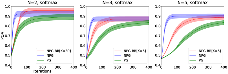
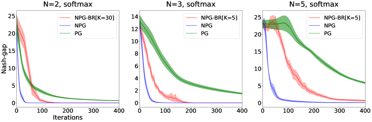
Figure 1: POA (top) and Nash-gap (bottom) under the tabular softmax parameterization (means and standard errors over 10 random initializations).The dashed lines are the curves of the log barrier regularized version of the algorithms with the same color.

We make Assumption 4.6 that also appears in the normal-form game setting (Roughgarden, 2015).

Assumption 4.6.

We have $0<\Phi_{\pi}(s)\leq V_{\pi}(s)$ for any product policy $\pi$ and any state $s$.

Theorem 4.7 (POA bound of maximum-gain $\epsilon$-ratio-best-response in smooth MPGs, proof in Appendix F.1).

Consider a $(\alpha,\beta)$-smooth MPG where Assumption 4.6 holds. Let $\pi_{*}=\operatorname*{arg\,max}_{\pi}V_{\pi}(\mu)$ be a globally optimal policy and $\sigma>0$ be a constant for analysis. Consider the sequence of maximum-gain $\epsilon$-ratio-best-response policies $\pi_{0},...,\pi_{T}$. Then, all but at most

$$\log_{\rho}{\frac{\Phi_{\rm max}}{\Phi_{0}}}-T\log_{\rho}{\frac{1}{1-\epsilon}}$$ (7)

policies $\pi_{t}$ in the sequence satisfy

$$V_{\pi_{t}}(\mu)\geq\frac{\alpha}{(1+\beta)(1+\sigma)}V_{\pi_{*}}(\mu)$$ (8)

where $\rho=(1-\epsilon)(1+\frac{\sigma(1+\beta)}{N})$ and $\Phi_{t}:=\Phi_{\pi_{t}}(\mu)$.

Since our NPG dynamics (5,3.3) described in Section 3.3 is an instance of maximum-gain approximate-best-response dynamics, we have Corollary 4.8 directly induced by Theorem 4.7.

Corollary 4.8 (POA bound of the approximate-best-response NPG dynamics (5,3.3) in smooth MPGs, proof in Appendix F.2).

Consider a $(\alpha,\beta)$-smooth MPG where Assumption 4.6 holds. Let $\pi_{*}=\operatorname*{arg\,max}_{\pi}V_{\pi}(\mu)$ be a globally optimal policy and $\sigma>0$ be a constant for analysis. Consider the sequence of policies $\pi_{0},...,\pi_{T}$ generated from the approximate-best-response NPG dynamics (5,3.3) with $K\geq\frac{4}{(1-\gamma)^{2}\epsilon}$. Then, all but at most

$$\log_{\rho}{\frac{\Phi_{\rm max}}{\Phi_{0}}}-T\log_{\rho}{\left(1+\frac{\epsilon}{2(1-\gamma)}\right)}$$ (9)

policies $\pi_{t}$ in the sequence satisfy (8), where $\rho=(1+\frac{\sigma(1+\beta)}{N})/(1+\frac{\epsilon}{2(1-\gamma)})$.

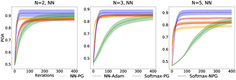
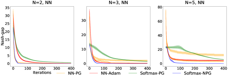
Figure 2: POA (top) and Nash-gap (bottom) under the NN parameterization (means and standard errors over 20 random initializations).The dashed lines are the curves of the log barrier regularized version of the algorithms with the same color.

5 Experiments

Environment. We evaluate the algorithms on Coordination Game, which extends the two players version in (Zhang et al., 2021) to multiple players $N=2,3,5$. The state space and action space are $\mathcal{S}=\mathcal{S}^{1}\times\cdots\times\mathcal{S}^{N},\mathcal{A}=\mathcal{A}^{1}\times\cdots\times\mathcal{A}^{N}$, respectively, where $\forall i\leq N,\mathcal{S}^{i}\in\{0,1\},\mathcal{A}^{i}\in\{0,1\}$. The reward is shared by all the agents (cooperative setting, a special case of Markov Potential Games), and it encourages agents to be in the same local state. To have rewards with more different levels, we design the reward in the way that when the number of agents occupy local state $0$ or $1$, whichever the maximum, to be the same, the state with more local states of $0$s is larger than the one with more $1$s. The transition function for each agent $i$’s local state is $P(s^{i}=0|a^{i}=0)=1-\epsilon$, $P(s^{i}=0|a^{i}=1)=\epsilon$, where $\epsilon=0.1$.

Algorithms. We exhaustively evaluate the performance of policy gradient PG, natural policy gradient NPG, and best response natural policy gradient NPG-BR with softmax parameterization under the tabular setting, w/wo log barrier regularizer. Besides softmax parameterization for PG, we also consider the neural network parameterization with softmax activation in the last layer NN-PG. Precisely, the policy gradient update rule for agent $i$’s neural network policy $\pi^{i}_{\theta^{i}}\colon\mathcal{S}\to\Delta(\mathcal{A}^{i})$ is

$$\nabla_{\theta^{i}}\Phi_{\theta}(\mu)=\sum_{s}\sum_{a^{i}}d_{\mu}^{\pi_{\theta}}(s)\pi^{i}_{\theta^{i}}(a^{i}|s)A^{i}_{\theta}(s,a^{i})\nabla_{\theta^{i}}\pi_{\theta^{i}}^{i}(a^{i}|s).$$

We run each algorithm in Coordination Game with $N=2,3,5$ agents and plot the Nash-gap and POA as the evaluation metrics. The algorithms, both the tabular softmax and the neural network parameterizations, share the same initial policy parameters, which are sampled from the normal distribution of mean 0 and standard deviation 1. For each log barrier regularized algorithm, we performed a grid search for its coefficient $\lambda\in\{0.01,0.1,1.0,10.0,100.0\}$ and picked the one with the best POA. Additional details of our experiment are presented in Appendix G.

5.1 Results under the tabular softmax parameterization

Figure 1 presents the POA and the Nash-gap of the algorithms under the tabular softmax parameterization. The results help address the following questions:

How fast do the algorithms converge? In terms of both the POA and the Nash-gap, NPG converges fastest, with NPG-BR the second and PG the slowest. This result demonstrates the improvement in the convergence rate of using the natural policy gradient over the policy gradient.

What is the effect of $K$ for NPG-BR? We did a grid search of $K\in\{1,5,10,20,50\}$ for NPG-BR (details in Appendix H.1), we show the results for the best-performing $K$ in terms of the POA for $N=2,3,5$ separately in Figure 1. We observe that $K=5$ is the best for $N=3,5$ and $K=50$, the largest value we searched, is the best for $N=2$.

How do the algorithms compare in terms of the POA? Consistent with the converge rate, NPG enjoys the overall highest POA, with NPG-BR the second and PG the lowest.

5.2 Results under the neural network parameterization

Figure 2 presents the POA and the Nash-gap of the algorithms under the neural network (NN) parameterization. The results help address the following questions:

Does NN help improve the convergence/POA from tabular softmax? With the NN parameterization, the PG algorithm (“NN-PG”) significantly outperforms its tabular softmax counterpart (“Softmax-PG”) in terms of both the convergence rate and the POA. NN-PG even outperforms Softmax-NPG in terms of POA at the beginning of the training, although and eventually the POA of Softmax-NPG is the highest among all. This demonstrates the significant improvement of the NN parameterization over the tabular softmax.

What is the effect of the NN regularization? Compared with the results under tabular softmax, the log barrier regularization under NN has a significantly larger impact: it both improves the POA and reduces the Nash-gap at convergence, especially when $N$ is large (e.g., $N=5$).

What is the effect of the NN optimizer? Among all NN variants, NN-PG is the best in terms of POA when $N$ is small, and the regularized NN-Adam is the best when $N$ is large. When $N=5$, the POA of the best NN variant, the regularized NN-Adam, is still significantly smaller than Softmax-NPG.

6 Conclusion and discussion

To conclude, we have established in Section 3 convergence to (near-)Nash policies in Markov potential games of several policy gradient-based dynamics under tabular softmax parameterization, including asymptotic convergence of the standard policy gradient dynamics (Section 3.1), its finite-time convergence with log-barrier regularization (Section 3.2), and finite-time convergence of the approximate best-response natural policy gradient dynamics (Section 3.3). In Section 4, we have extended the notion of smoothness in normal-form games to Markov games and established the price-of-anarchy bounds of near-Nash policies in smooth Markov games and of the approximate maximum-gain best-response dynamics in smooth Markov potential games.

Future work.

(i) Our theoretical guarantee for the NPG dynamics is limited to the (approximate) best-response variant, although our empirical results imply that the standard NPG dynamics where all agents get updated per iteration should also converge. This suggests that a future direction is to establish the convergence of the standard NPG dynamics. (ii) Our POA bound is also limited to the (approximate) best-response NPG dynamics, and a future direction is to provide POA bounds for other learning dynamics. (iii) Both the theoretical and the empirical parts of this paper are limited to exact gradient computation, and therefore an immediate future direction is to explore sample-based learning dynamics.

Appendix A Proof of Lemma 3.1

Note that

$$\frac{\partial\log{\pi^{i}_{\theta^{i}}(a^{i}_{\prime}|s^{\prime})}}{\partial\theta^{i}_{s,a^{i}}}=\mathbbm{1}[s=s^{\prime}](\mathbbm{1}[a^{i}=a^{i}_{\prime}]-\pi^{i}_{\theta^{i}}(a^{i}|s)).$$

Plugging it and by similar derivations in the proof of Lemma C.1 in (Agarwal et al., 2019), we have:

$$\frac{\partial V^{i}_{\theta}(\mu)}{\partial\theta^{i}_{s,a^{i}}}= \operatorname{\mathbb{E}}_{s^{\prime}\sim d^{\pi_{\theta}}_{\mu}}\operatorname{\mathbb{E}}_{a^{\prime}\sim\pi_{\theta}(\cdot|s)}\left[\mathbbm{1}[(s^{\prime},a^{i}_{\prime})=(s,a^{i})]A^{i}_{\theta}(s^{\prime},a^{\prime})\right]$$

$$= d^{\pi_{\theta}}_{\mu}(s)\pi^{i}_{\theta^{i}}(a^{i}|s)\operatorname{\mathbb{E}}_{a^{-i}\sim\pi^{-i}_{\theta^{-i}}(\cdot|s)}\left[A^{i}_{\theta}(s,a^{i},a^{-i})\right].$$

This concludes the proof.

Appendix B Proof of Lemma 3.2

Since $\Phi_{\theta}(s_{0})$, abbreviated as $\Phi_{\theta}$ in this proof, is (assumed to be) twice-differentialble, as an equivalent condition for smoothness, we will bound the spectral norm of its Hessian $\nabla^{2}_{\theta}\Phi_{\theta}$. Similar to the proof of Lemma 4.4 in (Leonardos et al., 2021), we view Hessian

$$\nabla^{2}_{\theta}\Phi_{\theta}=\left[\frac{\partial^{2}\Phi_{\theta}}{\partial\theta^{i}_{s,a^{i}}\partial\theta^{j}_{s^{\prime},a^{j}}}\right]_{i,s,a^{i},j,s^{\prime},a^{j}}$$

as a symmetric $N\times N$ block matrix with submatrices

$$\nabla^{2}_{\theta^{i}\theta^{j}}\Phi_{\theta}=\left[\frac{\partial^{2}\Phi_{\theta}}{\partial\theta^{i}_{s,a^{i}}\partial\theta^{j}_{s^{\prime},a^{j}}}\right]_{s,a^{i},s^{\prime},a^{j}}$$

for all $i,j\in\mathcal{N}$. Claim C.2 in (Leonardos et al., 2021) shows that if we can bound the spectral norm of any submatrix as $\left\lVert\nabla^{2}_{\theta^{i}\theta^{j}}\Phi_{\theta}\right\rVert_{2}\leq L$, then the spectral norm of the block matrix is bounded as $\left\lVert\nabla^{2}_{\theta}\Phi_{\theta}\right\rVert_{2}\leq NL$. We then next bound the spectural norm (i.e., the largest absolute eigenvalue) of matrix $\nabla^{2}_{\theta^{j}\theta^{i}}\Phi_{\theta}$. Noting $\nabla^{2}_{\theta^{j}\theta^{i}}\Phi_{\theta}=\nabla^{2}_{\theta^{j}\theta^{i}}V^{j}_{\theta}=\nabla^{2}_{\theta^{j}\theta^{i}}V^{i}_{\theta}$ due to (1), it suffices to define $U(t):=V_{\theta^{i}+t\cdot u,\theta^{-i}}$ and $W(t,s):=V_{\theta^{i}+t\cdot u,\theta^{j}+s\cdot v,\theta^{-i,-j}}$ for scalars $t,s\geq 0$ and unit vectors $u,v$, and to show

$$\max_{\left\lVert u\right\rVert_{2}=1}\left\lvert\left.\frac{d^{2}U(t)}{dt^{2}}\right|_{t=0}\right\rvert\leq\frac{41}{4(1-\gamma)^{3}}\text{ and }\max_{\left\lVert u\right\rVert_{2}=\left\lVert v\right\rVert_{2}=1}\left\lvert\left.\frac{d^{2}W(t,s)}{dtds}\right|_{t=0,s=0}\right\rvert\leq\frac{41}{4(1-\gamma)^{3}}.$$

For $U(t)$, we decompose it as $U(t)=\sum_{a^{i}}\sum_{a^{-i}}\pi^{i}_{\theta^{i}+t\cdot u}(a^{i}|s_{0})\cdot\pi^{-i}_{\theta^{-i}}(a^{-i}|s_{0})\cdot Q_{\theta^{i}+t\cdot u,\theta^{-i}}(s_{0},a^{i},a^{-i})$. Abbreviating $\pi^{i}_{\theta^{i}+t\cdot u}$ as $\pi^{i}_{t}$, $\pi^{-i}_{\theta^{-i}}$ as $\pi^{-i}$, and $Q_{\theta^{i}+t\cdot u,\theta^{-i}}$ as $Q_{t}$, we have

$$\frac{d^{2}U(t)}{dt^{2}}=\sum_{a^{i}}\sum_{a^{-i}}\bigg{(} \frac{d^{2}\pi^{i}_{t}(a^{i}|s_{0})}{dt^{2}}\cdot\pi^{-i}(a^{-i}|s_{0})\cdot Q_{t}(s_{0},a^{i},a^{-i})$$

$$+ 2\frac{d\pi^{i}_{t}(a^{i}|s_{0})}{dt}\cdot\pi^{-i}(a^{-i}|s_{0})\cdot\frac{dQ_{t}(s_{0},a^{i},a^{-i})}{dt}$$

$$+ \pi^{i}_{t}(a^{i}|s_{0})\cdot\pi^{-i}(a^{-i}|s_{0})\cdot\frac{d^{2}Q_{t}(s_{0},a^{i},a^{-i})}{dt^{2}}\bigg{)}$$

We then bound $\left\lvert\left.\frac{d^{2}U(t)}{dt^{2}}\right|_{t=0}\right\rvert$ for any unit vector $u$ by bounding the three terms, respectively. For the first term, we have $\sum_{a^{i}}\left\lvert\left.\frac{d^{2}\pi^{i}_{t}(a^{i}|s_{0})}{dt^{2}}\right|_{t=0}\right\rvert\leq 6=:C_{2}$ as proved in Lemma D.4 in (Agarwal et al., 2019), $0\leq Q_{t}(s_{0},a^{i},a^{-i})\leq\frac{1}{1-\gamma}$ assuming the reward is bounded in $[0,1]$, and $\sum_{a^{-i}}\pi^{-i}(a^{-i}|s_{0})=1$. For the second term, we have $\sum_{a^{i}}\left\lvert\left.\frac{d\pi^{i}_{t}(a^{i}|s_{0})}{dt}\right|_{t=0}\right\rvert\leq 2=:C_{1}$ as proved in Lemma D.4 in (Agarwal et al., 2019), and $\left\lvert\left.\frac{dQ_{t}(s_{0},a^{i},a^{-i})}{dt}\right|_{t=0}\right\rvert\leq\frac{\gamma C_{1}}{(1-\gamma)^{2}}$ as proved in Lemma D.2 in (Agarwal et al., 2019) and Lemma 4.4 in (Leonardos et al., 2021). For the third term, we have $\left\lvert\left.\frac{d^{2}Q_{t}(s_{0},a^{i},a^{-i})}{dt^{2}}\right|_{t=0}\right\rvert\leq\frac{2\gamma^{2}C_{1}}{(1-\gamma)^{3}}+\frac{\gamma C_{2}}{(1-\gamma)^{2}}$ as proved in Lemma D.2 in (Agarwal et al., 2019). We hence derive the bound:

$$\max_{\left\lVert u\right\rVert_{2}=1}\left\lvert\left.\frac{d^{2}U(t)}{dt^{2}}\right|_{t=0}\right\rvert\leq \frac{C_{2}}{1-\gamma}+\frac{2\gamma C_{1}^{2}}{(1-\gamma)^{2}}+\frac{2\gamma^{2}C_{1}}{(1-\gamma)^{3}}+\frac{\gamma C_{2}}{(1-\gamma)^{2}}$$

$$= \frac{C_{2}}{(1-\gamma)^{2}}+\frac{2\gamma C_{1}^{2}}{(1-\gamma)^{3}}=\frac{6+2\gamma}{(1-\gamma)^{3}}\qquad\text{($C_{1}=2,C_{2}=6$)}$$

$$\leq \frac{8}{(1-\gamma)^{3}}\leq\frac{41}{4(1-\gamma)^{3}}$$

For $W(t,s)$, similarly, we decompose it as $W(t,s)=\sum_{a^{i}}\sum_{a^{j}}\sum_{a^{-i,-j}}\pi^{i}_{\theta^{i}+t\cdot u}(a^{i}|s_{0})\cdot\pi^{j}_{\theta^{j}+s\cdot v}(a^{j}|s_{0})\cdot\pi^{-i,-j}_{\theta^{-i,-j}}(a^{-i,-j}|s_{0})\cdot Q_{\theta^{i}+t\cdot u,\theta^{j}+s\cdot v,\theta^{-i,-j}}(s_{0},a^{i},a^{j},a^{-i,-j})$. With similar abbreviations, we have

$$\frac{d^{2}W(t,s)}{dtds}=\sum_{a^{i}}\sum_{a^{j}}\sum_{a^{-i,-j}}\bigg{(} \frac{d\pi^{i}_{t}(a^{i}|s_{0})}{dt}\cdot\frac{d\pi^{j}_{s}(a^{j}|s_{0})}{ds}\cdot\pi^{-i,-j}(a^{-i,-j}|s_{0})\cdot Q_{t,s}(s_{0},a^{i},a^{j},a^{-i,-j})$$

$$+ \frac{d\pi^{i}_{t}(a^{i}|s_{0})}{dt}\cdot\pi^{j}_{s}(a^{j}|s_{0})\cdot\pi^{-i,-j}(a^{-i,-j}|s_{0})\cdot\frac{dQ_{t,s}(s_{0},a^{i},a^{j},a^{-i,-j})}{ds}$$

$$+ \pi^{i}_{t}(a^{i}|s_{0})\cdot\frac{d\pi^{j}_{s}(a^{j}|s_{0})}{ds}\cdot\pi^{-i,-j}(a^{-i,-j}|s_{0})\cdot\frac{dQ_{t,s}(s_{0},a^{i},a^{j},a^{-i,-j})}{dt}$$

$$+ \pi^{i}_{t}(a^{i}|s_{0})\cdot\pi^{j}_{s}(a^{j}|s_{0})\cdot\pi^{-i,-j}(a^{-i,-j}|s_{0})\cdot\frac{d^{2}Q_{t,s}(s_{0},a^{i},a^{j},a^{-i,-j})}{dtds}\bigg{)}.$$

We then bound $\left\lvert\left.\frac{d^{2}W(t,s)}{dtds}\right|_{t=0,s=0}\right\rvert$ for any unit vectors $u,v$ by bounding the four terms, respectively. Similarly, the first term can be bounded by $\frac{C_{1}^{2}}{1-\gamma}$, the second term by $\frac{\gamma C_{1}^{2}}{(1-\gamma)^{2}}$, the third term by $\frac{\gamma C_{1}^{2}}{(1-\gamma)^{2}}$, and the fourth term by $\frac{C_{2}}{(1-\gamma)^{2}}+\frac{2\gamma C_{1}^{2}}{(1-\gamma)^{3}}$. We hence derive the bound:

$$\max_{\left\lVert u\right\rVert=\left\lVert v\right\rVert=1}\left\lvert\left.\frac{d^{2}W(t,s)}{dtds}\right|_{t=0,s=0}\right\rvert\leq \frac{C_{1}^{2}}{1-\gamma}+\frac{\gamma C_{1}^{2}}{(1-\gamma)^{2}}+\frac{\gamma C_{1}^{2}}{(1-\gamma)^{2}}+\frac{C_{2}}{(1-\gamma)^{2}}+\frac{2\gamma C_{1}^{2}}{(1-\gamma)^{3}}$$

$$= \frac{-4\gamma^{2}+2\gamma+10}{(1-\gamma)^{3}}\qquad\text{($C_{1}=2,C_{2}=6$)}$$

$$\leq \frac{41}{4(1-\gamma)^{3}}.$$

This concludes the proof.

Appendix C Proof of Theorem 3.4

C.1 Notation

Define

$$V_{\phi}^{\pi_{\theta}}(s)=\operatorname{\mathbb{E}}[\sum_{t=0}^{\infty}\gamma^{t}\phi(s_{t},a_{t})|\pi_{\theta},s_{0}=s]$$

$$\Phi^{\pi_{\theta}}(\mu)=\operatorname{\mathbb{E}}_{s_{0}\sim\mu}[V_{\phi}^{\pi_{\theta}}(s_{0})]$$

$$Q_{\phi}^{\pi_{\theta}}(s,a)=\operatorname{\mathbb{E}}[\sum_{t=0}^{\infty}\gamma^{t}\phi(s_{t},a_{t})|\pi_{\theta},s_{0}=s,a_{0}=a]$$

$$A_{\phi}^{\pi_{\theta}}(s,a)=Q_{\phi}^{\pi_{\theta}}(s,a)-V_{\phi}^{\pi_{\theta}}(s)$$

Suppose $\Phi_{\text{min}}\leq Q_{\phi}^{\pi_{\theta}}(s,a)\leq\Phi_{\text{max}}$.

C.2 Smoothness of F

Lemma C.1 (Smoothness of $F$ under tabular softmax).

Fix a state $s$. Let $\theta_{s}=[(\theta^{1}_{s})^{\top},...,(\theta^{N}_{s})^{\top}]^{\top}\in\mathbb{R}^{\sum_{i}|\mathcal{A}^{i}|}$ be the column vector of parameters for state $s$, with $\theta^{i}_{s}\in\mathbb{R}^{|\mathcal{A}^{i}|}$ for $i\in\mathcal{N}$. For some fixed vector $c_{s}\in\mathbb{R}^{|\mathcal{A}|}$, define $F_{s}(\theta_{s}):=\sum_{a\in\mathcal{A}}\pi_{\theta_{s}}(a|s)c_{s,a}=:\pi_{\theta_{s}}\cdot c_{s}$ with $\pi_{\theta_{s}}\in\mathbb{R}^{|\mathcal{A}|}$ and $\cdot$ denoting inner product. Then, $F_{s}(\theta_{s})$ is -smooth.

Proof.

We will view Hessian $\nabla^{2}_{\theta_{s}}F_{s}(\theta_{s})$ as a $N\times N$ block matrix and bound the spectral norm of each submatrix as $\left\lVert\nabla^{2}_{\theta^{i}_{s}\theta^{j}_{s}}F_{s}(\theta_{s})\right\rVert_{2}\leq L$, which bounds the Hessian’s spectral norm as $\left\lVert\nabla^{2}_{\theta_{s}}F_{s}(\theta_{s})\right\rVert_{2}\leq NL$.

We have

$$\nabla_{\theta^{i}_{s}}F_{s}(\theta_{s})=\nabla_{\theta^{i}_{s}}(\pi_{\theta_{s}}\cdot c_{s})=(\nabla_{\theta^{i}_{s}}\pi_{\theta_{s}})^{\top}c_{s}=\nabla_{\theta^{i}_{s}}\pi^{i}_{\theta^{i}_{s}}\left(\pi^{-i}_{\theta^{-i}_{s}}\otimes I_{|\mathcal{A}^{i}|}\right)^{\top}M^{i}c_{s}$$

where $\nabla_{\theta^{i}_{s}}F_{s}(\theta_{s})\in\mathbb{R}^{1\times|\mathcal{A}^{i}|}$, $M^{i}\in\mathbb{R}^{|\mathcal{A}|\times|\mathcal{A}|}$ is the permutation matrix that permutes all joint actions to be sorted as $a=(a^{-i},a^{i})$, $I_{n}$ is the $n\times n$ identity matrix, and $\otimes$ is the Kronecker product. For the tabular softmax parameterization, we have

$$\nabla_{\theta^{i}_{s}}\pi^{i}_{\theta^{i}_{s}}={\rm diag}\left(\pi^{i}_{\theta^{i}_{s}}\right)-\pi^{i}_{\theta^{i}_{s}}\left(\pi^{i}_{\theta^{i}_{s}}\right)^{\top}.$$

The submatrix is therefore

$$\nabla^{2}_{\theta^{i}_{s}\theta^{j}_{s}}F_{s}(\theta_{s})= \nabla_{\theta^{j}_{s}}\left(\nabla_{\theta^{i}_{s}}\pi^{i}_{\theta^{i}_{s}}\left(\pi^{-i}_{\theta^{-i}_{s}}\otimes I_{|\mathcal{A}^{i}|}\right)^{\top}M^{i}c_{s}\right)$$

If $j=i$:

$$\nabla^{2}_{\theta^{i}_{s}\theta^{i}_{s}}F_{s}(\theta_{s})= \nabla_{\theta^{i}_{s}}\left(\nabla_{\theta^{i}_{s}}\pi^{i}_{\theta^{i}_{s}}\left(\pi^{-i}_{\theta^{-i}_{s}}\otimes I_{|\mathcal{A}^{i}|}\right)^{\top}M^{i}c_{s}\right)$$

$$= \nabla_{\theta^{i}_{s}}(\pi^{i}_{\theta^{i}_{s}}\odot b-(\pi^{i}_{\theta^{i}_{s}}\cdot b)\pi^{i}_{\theta^{i}_{s}})$$

, where $b=\left(\pi^{-i}_{\theta^{-i}_{s}}\otimes I_{|\mathcal{A}^{i}|}\right)^{\top}M^{i}c_{s}.$
For the first term, we get

$$\nabla_{\theta^{i}_{s}}(\pi^{i}_{\theta^{i}_{s}}\odot b)=\text{diag}(\pi^{i}_{\theta^{i}_{s}}\odot b)-\pi^{i}_{\theta^{i}_{s}}(\pi^{i}_{\theta^{i}_{s}}\odot b)^{\top}$$

For the second term we get:

$$\nabla_{\theta^{i}_{s}}((\pi^{i}_{\theta^{i}_{s}}\cdot b)\pi^{i}_{\theta^{i}_{s}})=(\pi^{i}_{\theta^{i}_{s}}\cdot b)\nabla_{\theta^{i}_{s}}(\pi^{i}_{\theta^{i}_{s}})+(\nabla_{\theta^{i}_{s}}(\pi^{i}_{\theta^{i}_{s}}\cdot b))(\pi^{i}_{\theta^{i}_{s}})^{\top}$$

$$\longrightarrow\nabla^{2}_{\theta^{i}_{s}\theta^{i}_{s}}F_{s}(\theta_{s})=\text{diag}(\pi^{i}_{\theta^{i}_{s}}\odot b)-\pi^{i}_{\theta^{i}_{s}}(\pi^{i}_{\theta^{i}_{s}}\odot b)^{\top}-(\pi^{i}_{\theta^{i}_{s}}\cdot b)\nabla_{\theta^{i}_{s}}(\pi^{i}_{\theta^{i}_{s}})-(\nabla_{\theta^{i}_{s}}(\pi^{i}_{\theta^{i}_{s}}\cdot b))(\pi^{i}_{\theta^{i}_{s}})^{\top}$$

Since

$$\text{max}(\left\lVert\text{diag}(\pi^{i}_{\theta^{i}_{s}}\odot b)\right\rVert_{2},\left\lVert\pi^{i}_{\theta^{i}_{s}}\odot b\right\rVert_{2},|\pi^{i}_{\theta^{i}_{s}}\cdot b|)\leq\left\lVert b\right\rVert_{\infty}=\left\lVert c\right\rVert_{\infty}$$

$$\left\lVert\nabla_{\theta^{i}_{s}}\pi^{i}_{\theta^{i}_{s}}\right\rVert_{2}=\left\lVert{\rm diag}\left(\pi^{i}_{\theta^{i}_{s}}\right)-\pi^{i}_{\theta^{i}_{s}}\left(\pi^{i}_{\theta^{i}_{s}}\right)^{\top}\right\rVert_{2}\leq 1$$

$$\left\lVert\nabla_{\theta^{i}_{s}}(\pi^{i}_{\theta^{i}_{s}}\cdot b)\right\rVert_{2}\leq\left\lVert\pi^{i}_{\theta^{i}_{s}}\odot b\right\rVert_{2}+\left\lVert(\pi^{i}_{\theta^{i}_{s}}\cdot b)\pi^{i}_{\theta^{i}_{s}}\right\rVert_{2}\leq 2\left\lVert c\right\rVert_{\infty},$$

we know that

$$\left\lVert\nabla^{2}_{\theta^{i}_{s}\theta^{i}_{s}}F_{s}(\theta_{s})\right\rVert_{2}\leq 5\left\lVert c\right\rVert_{\infty}$$

If $j\neq i$:

$$\nabla^{2}_{\theta^{i}_{s}\theta^{j}_{s}}F_{s}(\theta_{s})= M^{j}\nabla_{\theta^{i}_{s}}\pi^{i}_{\theta^{i}_{s}}\Bigg{(}\bigg{(}\Big{(}\pi^{-i,-j}_{\theta^{-i,-j}_{s}}\otimes I_{|\mathcal{A}^{j}|}\Big{)}\nabla_{\theta^{j}_{s}}\pi^{j}_{\theta^{j}_{s}}\bigg{)}\otimes I_{|\mathcal{A}^{i}|}\Bigg{)}^{\top}M^{j}M^{i}c_{s}$$

Since
$\left\lVert M^{j}M^{i}c_{s}\right\rVert_{2}\leq\sqrt{N}\left\lVert c\right\rVert_{\infty}$

$$\begin{split}\left\lVert\bigg{(}\Big{(}\pi^{-i,-j}_{\theta^{-i,-j}_{s}}\otimes I_{|\mathcal{A}^{j}|}\Big{)}\nabla_{\theta^{j}_{s}}\pi^{j}_{\theta^{j}_{s}}\bigg{)}\otimes I_{|\mathcal{A}^{i}|}\right\rVert_{2}&=\left\lVert\Big{(}\pi^{-i,-j}_{\theta^{-i,-j}_{s}}\otimes I_{|\mathcal{A}^{j}|}\Big{)}\nabla_{\theta^{j}_{s}}\pi^{j}_{\theta^{j}_{s}}\right\rVert_{2}\\ &\leq\left\lVert\pi^{-i,-j}_{\theta^{-i,-j}_{s}}\otimes I_{|\mathcal{A}^{j}|}\right\rVert_{2}\left\lVert\nabla_{\theta^{j}_{s}}\pi^{j}_{\theta^{j}_{s}}\right\rVert_{2}\\ &\leq\left\lVert\pi^{-i,-j}_{\theta^{-i,-j}_{s}}\right\rVert_{2}\\ &\leq 1\end{split}$$ (10)

we know that

$$\nabla^{2}_{\theta^{i}_{s}\theta^{j}_{s}}F_{s}(\theta_{s})\leq\sqrt{N}\left\lVert c\right\rVert_{\infty}$$

∎

Therefore, we have

$$\left\lVert\nabla^{2}_{\theta_{s}}F_{s}(\theta_{s})\right\rVert_{2}\leq N\text{max}(5,\sqrt{N})\left\lVert c\right\rVert_{\infty}$$

Lemma C.2.

For product policy that can be factorized into the product of individual policies with softmax parameterization, we have:

$$\frac{\partial V^{\pi_{\theta}}(\mu)}{\partial\theta_{s,a^{i}}^{i}}=\frac{\partial\Phi^{\pi_{\theta}}(\mu)}{\partial\theta_{s,a^{i}}^{i}}=\frac{1}{1-\gamma}d_{\mu}^{\pi_{\theta}}(s)\pi_{\theta^{i}}(a^{i}|s)A_{\phi}^{\pi_{\theta},i}(s,a^{i})$$

,where $Q_{\phi}^{\pi_{\theta},i}(s,a^{i})=\operatorname{\mathbb{E}}_{a^{-i}\sim\pi_{\theta^{-i}}(\cdot|s)}\Big{[}Q_{\phi}^{\pi_{\theta}}(s,a^{i},a^{-i})\Big{]},A_{\phi}^{\pi_{\theta},i}(s,a^{i})=Q_{\phi}^{\pi_{\theta},i}(s,a^{i})-V_{\phi}^{\pi_{\theta}}(s).$

Proof.

$$\frac{\partial V_{\phi}^{\pi_{\theta}}(\mu)}{\partial\theta_{s^{\prime},a^{i}}^{i}}=\frac{\partial\Phi^{\pi_{\theta}}(\mu)}{\partial\theta_{s,a^{i}}^{i}}=\frac{1}{1-\gamma}\operatorname{\mathbb{E}}_{s\sim d_{\mu}^{\pi_{\theta}}}\operatorname{\mathbb{E}}_{a\sim\pi_{\theta}(\cdot|s)}\Big{[}A_{\phi}^{\pi_{\theta}}(s,a)\frac{\partial\log\pi_{\theta^{i}}(a^{i}|s)}{\partial\theta_{s^{\prime},a^{i}}^{i}}\Big{]}$$

$$=\frac{1}{1-\gamma}\operatorname{\mathbb{E}}_{s\sim d_{\mu}^{\pi_{\theta}}}\operatorname{\mathbb{E}}_{a\sim\pi_{\theta}(\cdot|s)}\Big{[}A_{\phi}^{\pi_{\theta}}(s,a)\mathbbm{1}[s=s^{\prime}](\mathbbm{1}[a[m]=a^{i}]-\pi_{\theta^{i}}(a^{i}|s))\Big{]}$$

$$=\frac{1}{1-\gamma}d_{\mu}^{\pi_{\theta}}(s^{\prime})\operatorname{\mathbb{E}}_{a\sim\pi_{\theta}(\cdot|s^{\prime})}\Big{[}A_{\phi}^{\pi_{\theta}}(s^{\prime},a)(\mathbbm{1}[a[m]=a^{i}]-\pi_{\theta^{i}}(a^{i}|s^{\prime}))\Big{]}$$

$$=\frac{1}{1-\gamma}d_{\mu}^{\pi_{\theta}}(s^{\prime})(\operatorname{\mathbb{E}}_{a\sim\pi_{\theta}(\cdot|s^{\prime})}\Big{[}A_{\phi}^{\pi_{\theta}}(s^{\prime},a)\mathbbm{1}[a[m]=a^{i}]\Big{]}-\operatorname{\mathbb{E}}_{a\sim\pi_{\theta}(\cdot|s^{\prime})}\Big{[}A_{\phi}^{\pi_{\theta}}(s^{\prime},a)\pi_{\theta^{i}}(a^{i}|s^{\prime})\Big{]})$$

$$=\frac{1}{1-\gamma}d_{\mu}^{\pi_{\theta}}(s^{\prime})(\operatorname{\mathbb{E}}_{a\sim\pi_{\theta}(\cdot|s^{\prime})}\Big{[}A_{\phi}^{\pi_{\theta}}(s^{\prime},a)\mathbbm{1}[a[m]=a^{i}]\Big{]}-\pi_{\theta^{i}}(a^{i}|s^{\prime})\operatorname{\mathbb{E}}_{a\sim\pi_{\theta}(\cdot|s^{\prime})}\Big{[}A_{\phi}^{\pi_{\theta}}(s^{\prime},a)\Big{]})$$

$$=\frac{1}{1-\gamma}d_{\mu}^{\pi_{\theta}}(s^{\prime})\operatorname{\mathbb{E}}_{a\sim\pi_{\theta}(\cdot|s^{\prime})}\Big{[}A_{\phi}^{\pi_{\theta}}(s^{\prime},a)\mathbbm{1}[a[m]=a^{i}]\Big{]}$$

$$=\frac{1}{1-\gamma}d_{\mu}^{\pi_{\theta}}(s^{\prime})\sum_{a}\pi_{\theta}(a|s^{\prime})A_{\phi}^{\pi_{\theta}}(s^{\prime},a)\mathbbm{1}[a[m]=a^{i}]$$

$$=\frac{1}{1-\gamma}d_{\mu}^{\pi_{\theta}}(s^{\prime})\pi_{\theta^{i}}(a^{i}|s^{\prime})\operatorname{\mathbb{E}}_{a^{-i}\sim\pi_{\theta}(\cdot|s^{\prime})}\Big{[}A_{\phi}^{\pi_{\theta}}(s^{\prime},a^{i},a^{-i})\Big{]}$$

$$=\frac{1}{1-\gamma}d_{\mu}^{\pi_{\theta}}(s^{\prime})\pi_{\theta^{i}}(a^{i}|s^{\prime})A_{\phi}^{\pi_{\theta},i}(s^{\prime},a^{i})$$

∎

Lemma C.3.

For all agents $i$ with a round of parallel update

$$\theta^{i}_{t+1}=\theta^{i}_{t}+\eta\nabla V^{i}_{\theta^{i}_{t}}(\mu)=\theta^{i}_{t}+\eta\nabla\Phi_{\theta^{i}_{t}}(\mu)$$

with learning rates $\eta\leq\frac{1-\gamma}{\beta}$, where $\beta=NL(\Phi_{\text{max}}-\Phi_{\text{min}})$ , $L=\text{max}(5,\sqrt{N})$, we have

$$V_{\phi}^{(t+1)}(s)\geq V_{\phi}^{(t)}(s);Q_{\phi}^{(t+1)}(s,a)\geq Q_{\phi}^{(t)}(s,a).$$

Proof.

Let us use the notation $\theta_{s}\in\mathbb{R}^{\sum_{i}|\mathcal{A}_{\phi}^{i}|}$ to refer to the parameters of the product policy on state $s$. Define

$$F_{s}(\theta_{s})=\sum_{a}\pi_{\theta_{s}}(a|s)c(s,a)$$

where $c(s,a)$ is treated as a constant, and is set to be $A_{\phi}^{(t)}(s,a)$ later in the proof. Thus,

$$\frac{\partial F_{s}(\theta_{s})}{\partial\theta_{s,a^{i}}^{i}}\bigg{|}_{\theta_{s}^{t,i}}=\sum_{a^{\prime}}\frac{\partial\pi_{\theta_{s}}(a^{\prime}|s)}{\partial\theta_{s,a^{i}}^{i}}\bigg{|}_{\theta_{s}^{t,i}}c(s,a^{\prime})$$

$$=\underbrace{\sum_{a^{\prime}}\mathbbm{1}[a^{\prime}[i]=a^{i}]\frac{\partial\pi_{\theta_{s}}(a^{\prime}|s)}{\partial\theta_{s,a^{i}}^{i}}\bigg{|}_{\theta_{s}^{t,i}}c(s,a^{\prime})}_{(1)}+\underbrace{\sum_{a^{\prime}}\mathbbm{1}[a^{\prime}[i]\neq a^{i}]\frac{\partial\pi_{\theta_{s}}(a^{\prime}|s)}{\partial\theta_{s,a^{i}}^{i}}\bigg{|}_{\theta_{s}^{t,i}}c(s,a^{\prime})}_{(2)}$$

$$(1)=\sum_{a^{\prime}}\mathbbm{1}[a^{\prime}[i]=a^{i}]\frac{\pi_{\theta_{s}}(a^{\prime}|s)}{\pi_{\theta_{s}^{i}}(a^{i}|s)}\Big{[}\pi_{\theta_{s}^{i}}(a^{i}|s)(1-\pi_{\theta_{s}^{i}}(a^{i}|s))\Big{]}c(s,a^{\prime})$$

$$=\sum_{a^{\prime}}\mathbbm{1}[a^{\prime}[i]=a^{i}]\pi_{\theta_{s}}(a^{\prime}|s)\Big{(}1-\pi_{\theta_{s}^{i}}(a^{i}|s)\Big{)}\bigg{|}_{\theta_{s,t}}c(s,a^{\prime})$$

$$=\sum_{a^{\prime}}\mathbbm{1}[a^{\prime}[i]=a^{i}]\pi^{t}(a^{\prime}|s)\Big{(}1-\pi^{t,i}(a^{i}|s)\Big{)}c(s,a^{\prime})$$

$$(2)=\sum_{a^{\prime}}\mathbbm{1}[a^{\prime}[i]\neq a^{i}]\frac{\pi_{\theta_{s}}(a^{\prime}|s)}{\pi_{\theta_{s}^{i}}(a^{i}|s)}\Big{(}-\pi_{\theta_{s}^{i}}(a^{i}|s)\pi_{\theta_{s}^{i}}(a^{\prime}[i]|s)\Big{)}\bigg{|}_{\theta_{s}^{t,i}}c(s,a^{\prime})$$

$$=-\sum_{a^{\prime}}\mathbbm{1}[a^{\prime}[i]\neq a^{i}]\pi_{\theta_{s}}(a^{\prime}|s)\pi_{\theta_{s}^{i}}(a^{i}|s)\bigg{|}_{\theta_{s}^{t,i}}c(s,a^{\prime})$$

$$=-\sum_{a^{\prime}}\mathbbm{1}[a^{\prime}[i]\neq a^{i}]\pi^{t}(a^{\prime}|s)\pi^{t,i}(a^{i}|s)c(s,a^{\prime})$$

$(1)+(2)=\sum_{a^{\prime}}\mathbbm{1}[a^{\prime}[i]=a^{i}]\pi^{t}(a^{\prime}|s)c(s,a^{\prime})-$

$$\Big{(}\sum_{a^{\prime}}\mathbbm{1}[a^{\prime}[i]=a^{i}]\pi^{t}(a^{\prime}|s)\pi^{t,i}(a^{i}|s)c(s,a^{\prime})+\sum_{a^{\prime}}\mathbbm{1}[a^{\prime}[i]\neq a^{i}]\pi^{t}(a^{\prime}|s)\pi^{t,i}(a^{i}|s)c(s,a^{\prime})\Big{)}$$

$$=\sum_{a^{\prime}}\mathbbm{1}[a^{\prime}[i]=a^{i}]\pi^{t}(a^{\prime}|s)c(s,a^{\prime})-\sum_{a^{\prime}}\pi^{t}(a^{\prime}|s)\pi^{t,i}(a^{i}|s)c(s,a^{\prime})$$

Let $c(s,a^{\prime})=A_{\phi}(s,a^{\prime})$,

$$=\sum_{a^{\prime}}\mathbbm{1}[a^{\prime}[i]=a^{i}]\pi^{t}(a^{\prime}|s)A_{\phi}(s,a^{\prime})-\sum_{a^{\prime}}\pi^{t}(a^{\prime}|s)\pi^{t,i}(a^{i}|s)A_{\phi}(s,a^{\prime})$$

$$=\sum_{a^{\prime}}\mathbbm{1}[a^{\prime}[i]=a^{i}]\pi^{t}(a^{\prime}|s)A_{\phi}(s,a^{\prime})$$

$$=\pi_{\theta^{i}}(a^{i}|s)A_{\phi}^{\pi_{\theta},i}(s,a^{i})$$

Therefore,

$$\nabla\Phi_{\theta^{i}}^{t}(\mu)=\frac{1}{1-\gamma}d_{\mu}^{\pi_{\theta}}(s)\frac{\partial F_{s}(\theta_{s})}{\partial\theta_{s,a^{i}}^{i}}$$

$$\longrightarrow\theta_{s}^{t+1}=\theta_{s}^{t}+\eta\frac{1}{1-\gamma}d_{\mu}^{\pi_{\theta}}(s)\frac{\partial F_{s}(\theta_{s})}{\partial\theta_{s}}\bigg{|}_{\theta_{s}^{t}}$$

Since $F_{s}(\theta_{s})$ is a $\beta$-smooth function for $\beta=N\text{max}(5,\sqrt{N})(\Phi_{\text{max}}-\Phi_{\text{min}})$, then our assumptions that $\eta\leq\frac{1-\gamma}{\beta}=\frac{1-\gamma}{N\text{max}(5,\sqrt{N})(\Phi_{\text{max}}-\Phi_{\text{min}})}$ implies $\eta\frac{1}{1-\gamma}d_{\mu}^{\pi_{\theta}}(s)\leq\frac{1}{\beta}$, which means

$$F_{s}(\theta_{s}^{t+1})\geq F_{s}(\theta_{s}^{t})$$

$$\longrightarrow V_{\phi}^{(t+1)}(s)\geq V_{\phi}^{(t)}(s);Q_{\phi}^{(t+1)}(s,a)\geq Q_{\phi}^{(t)}(s,a).$$

∎

Lemma C.4.

For all states s and actions a, there exists values $V_{\phi}^{\infty}(s),Q_{\phi}^{\infty}(s,a)\text{ and }Q_{\phi}^{\infty,i}(s,a)$ such that as $t\rightarrow\infty,V_{\phi}^{t}(s)\rightarrow V_{\phi}^{\infty}(s),Q_{\phi}^{t}(s,a)\rightarrow Q_{\phi}^{\infty}(s,a),Q_{\phi}^{t,i}(s,a)\rightarrow Q_{\phi}^{\infty,i}(s,a)$. Define

$$\Delta^{i}=\min_{\{s,a^{i}|A_{\phi}^{\infty,i}(s,a^{i})\neq 0\}}|A_{\phi}^{\infty,i}(s,a^{i})|.$$

$$\Delta=\min_{i}\Delta^{i}.$$

Further, there exists a $T_{0}$ such that $\forall t>T_{0},s\in\mathcal{S},a^{i}\in\mathcal{A}_{\phi}^{i},$

$$Q_{\phi}^{\infty,i}(s,a^{i})-\frac{\Delta}{4}\leq Q_{\phi}^{t,i}(s,a^{i})\leq Q_{\phi}^{\infty,i}(s,a^{i})+\frac{\Delta}{4}$$

Proof.

$\{V_{\phi}^{t}(s)\}$ is bounded and monotonically increasing, therefore $V_{\phi}^{t}(s)\rightarrow V_{\phi}^{\infty}(s)$. Similarly, we know $Q_{\phi}^{t}(s,a)\rightarrow Q_{\phi}^{\infty}(s,a)$. Since the product policy is assumed to converge, we have that $\{Q_{\phi}^{t,i}(s,a^{i})\}$ is convergent. For agent $i$, state $s$, categorize the local action $a^{i}$ into three groups:

$$I_{0}^{s,i}=\Bigg{\{}a^{i}|Q_{\phi}^{\infty,i}(s,a^{i})=V_{\phi}^{\infty}(s)\Bigg{\}}$$

$$I_{+}^{s,i}=\Bigg{\{}a^{i}|Q_{\phi}^{\infty,i}(s,a^{i})>V_{\phi}^{\infty}(s)\Bigg{\}}$$

$$I_{-}^{s,i}=\Bigg{\{}a^{i}|Q_{\phi}^{\infty,i}(s,a^{i})<V_{\phi}^{\infty}(s)\Bigg{\}}$$

Since $Q_{\phi}^{t,i}(s,a^{i})\rightarrow Q_{\phi}^{\infty,i}(s,a^{i})$ as $t\rightarrow\infty$, there exists a $T_{0}$ such that $\forall t>T_{0},s\in\mathcal{S},a^{i}\in\mathcal{A}_{\phi}^{i},$

$$Q_{\phi}^{\infty,i}(s,a^{i})-\frac{\Delta}{4}\leq Q_{\phi}^{t,i}(s,a^{i})\leq Q_{\phi}^{\infty,i}(s,a^{i})+\frac{\Delta}{4}$$

∎

Lemma C.5.

$\exists T_{1}$ such that $\forall t>T_{1},s\in\mathcal{S},$ we have

$$A_{\phi}^{t,i}(s,a^{i})<-\frac{\Delta}{4}\text{ for }a^{i}\in I_{-}^{s,i};A_{\phi}^{t,i}(s,a^{i})>\frac{\Delta}{4}\text{ for }a^{i}\in I_{+}^{s,i}$$

Proof.

Since $V_{\phi}^{t}(s)\rightarrow V_{\phi}^{\infty}(s)$, we have that there exists $T_{1}>T_{0}$ such that for all $t>T_{1}$,

$$V_{\phi}^{\infty}(s)-\frac{\Delta}{4}\leq V_{\phi}^{t}(s)\leq V_{\phi}^{\infty}(s)+\frac{\Delta}{4}$$

For $a^{i}\in I_{-}^{s,i},t>T_{1}>T_{0},$

$$\begin{split}A_{\phi}^{t,i}(s,a^{i})&=Q_{\phi}^{t,i}(s,a^{i})-V_{\phi}^{t}(s)\\ &\leq Q_{\phi}^{\infty,i}(s,a^{i})+\frac{\Delta}{4}-V_{\phi}^{t}(s)\\ &\leq Q_{\phi}^{\infty,i}(s,a^{i})+\frac{\Delta}{4}-V_{\phi}^{\infty}(s)+\frac{\Delta}{4}\\ &\leq-\Delta+\frac{\Delta}{4}+\frac{\Delta}{4}\\ &\leq-\frac{\Delta}{4}\end{split}$$ (11)

For $a^{i}\in I_{+}^{s,i},t>T_{1}>T_{0},$

$$\begin{split}A_{\phi}^{t,i}(s,a^{i})&=Q_{\phi}^{t,i}(s,a^{i})-V_{\phi}^{t}(s)\\ &\geq Q_{\phi}^{\infty,i}(s,a^{i})-\frac{\Delta}{4}-V_{\phi}^{t}(s)\\ &\geq Q_{\phi}^{\infty,i}(s,a^{i})-\frac{\Delta}{4}-V_{\phi}^{\infty}(s)\\ &\geq\Delta-\frac{\Delta}{4}\\ &\geq\frac{\Delta}{4}\end{split}$$ (12)

∎

Lemma C.6.

$\frac{\partial\Phi^{\pi_{\theta}}(\mu)}{\partial\theta_{s,a^{i}}^{i}}\rightarrow 0\text{ as }t\rightarrow\infty$ for all states $s$, agents $i$, actions $a^{i}$. This implies that $\forall a^{i}\in I_{-}^{s,i}\cup I_{+}^{s,i},\pi^{t,i}(a^{i}|s)\rightarrow 0$ and that $\sum_{a^{i}\in I_{0}^{s,i}}\pi^{t,i}(a^{i}|s)\rightarrow 1$.

Proof.

Since $\Phi^{\pi_{\theta}}(\mu)$ is smooth, we know $\frac{\partial\Phi^{\pi_{\theta}}(\mu)}{\partial\theta_{s,a^{i}}^{i}}\rightarrow 0$ for all $s,i,a^{i}$. From lemma 1 we have

$$\frac{\partial\Phi^{t}(\mu)}{\partial\theta_{s,a^{i}}^{i}}=\frac{1}{1-\gamma}d_{\mu}^{\pi^{t}}(s)\pi^{t,i}(a^{i}|s)A_{\phi}^{\pi^{t,i}}(s,a^{i})$$

Since from lemma 4 we know that $|A_{\phi}^{t,i}(s,a^{i})|>\frac{\Delta}{4}$ for all $t>T_{1}$, for all $a^{i}\in I_{-}^{s,i}\cup I_{+}^{s,i}$ , which together with the assumption that $\mu$ is strict positive for all state $s$ prove $\pi^{t,i}(a^{i}|s)\rightarrow 0$. Then we also know for all $\sum_{a^{i}\in I_{0}^{s,i}}\pi^{t,i}(a^{i}|s)\rightarrow 1$. ∎

Lemma C.7.

For $t\geq T_{1}$, $\theta_{s,a^{i}}^{i}$ is strictly decreasing $\forall a^{i}\in I_{-}^{s,i}$ and $\theta_{s,a^{i}}^{i}$ is strictly increasing $\forall a^{i}\in I+^{s,i}$.

Proof.

From lemma 1 we have

$$\frac{\partial\Phi^{t}(\mu)}{\partial\theta_{s,a^{i}}^{i}}=\frac{1}{1-\gamma}d_{\mu}^{\pi^{t}}(s)\pi^{t,i}(a^{i}|s)A_{\phi}^{{t,i}}(s,a^{i})$$

From lemma 4, we know for all $t>T_{1},a^{i}\in I_{-}^{s,i},A_{\phi}^{t,i}(s,a^{i})\leq-\frac{\Delta}{4};$ For all $a^{i}\in I_{+}^{s,i},A_{\phi}^{t,i}(s,a^{i})\geq\frac{\Delta}{4}.$ This implies that after iteration $T_{1}$, $\frac{\partial\Phi^{t}(\mu)}{\partial\theta_{s,a^{i}}^{i}}<0\forall a^{i}\in I_{-}^{s,i};\frac{\partial\Phi^{t}(\mu)}{\partial\theta_{s,a^{i}}^{i}}>0\forall a^{i}\in I_{+}^{s,i}.\longrightarrow$ After iteration $T_{1}$, $\theta_{s,a^{i}}^{i}$ is strictly decreasing $\forall a^{i}\in I_{-}^{s,i}$ and $\theta_{s,a^{i}}^{i}$ is strictly increasing $\forall a^{i}\in I_{+}^{s,i}$. ∎

Lemma C.8.

For all states $s$ where $I_{+}^{s,i}\neq\emptyset$, we have:

$$\text{max}_{a^{i}\in I_{0}^{s,i}}\theta_{s,a^{i}}^{t,i}\rightarrow\infty,\text{ min}_{a^{i}\in\mathbb{A}^{i}}\theta_{s,a^{i}}^{t,i}\rightarrow-\infty$$

Proof.

Since $I_{+}^{s,i}\neq\emptyset$, we have some action $a_{+}^{i}\in I_{+}^{s,i}$. From lemma 5, we know

$$\pi^{t,i}(a^{i}_{+}|s)\rightarrow 0\text{ as }t\rightarrow\infty$$

$$\longrightarrow\frac{\text{exp}(\theta_{s,a_{+}^{i}}^{t,i})}{\sum_{a^{i}\in\mathbb{A}^{i}}\text{exp}(\theta_{s,a^{i}}^{t,i})}\rightarrow 0\text{ as }t\rightarrow\infty$$

From lemma 6 we know $\theta_{s,a_{+}^{i}}^{t,i}$ is monotonically increasing, which implies

$$\sum_{a^{i}\in\mathbb{A}^{i}}\text{exp}(\theta_{s,a^{i}}^{t,i})\rightarrow\infty\text{ as }t\rightarrow\infty$$

From lemma 5, we also know

$$\sum_{a^{i}\in I_{0}^{s,i}}\pi^{t,i}(a^{i}|s)\rightarrow 1$$

$$\longrightarrow\frac{\sum_{a^{i}\in I_{0}^{s,i}}\text{exp}(\theta_{s,a^{i}}^{t,i})}{\sum_{a^{i}\in\mathbb{A}^{i}}\text{exp}(\theta_{s,a^{i}}^{t,i})}\rightarrow 1$$

Since denominator does to $\infty$, we know

$$\sum_{a^{i}\in I_{0}^{s,i}}\text{exp}(\theta_{s,a^{i}}^{t,i})\rightarrow\infty$$

which implies

$$\text{max}_{a^{i}\in I_{0}^{s,i}}\theta_{s,a^{i}}^{t,i}\rightarrow\infty$$

Note this also implies $\text{max}_{a^{i}\in\mathbb{A}^{i}}\theta_{s,a^{i}}^{t,i}\rightarrow\infty$. The sum of the gradient is always zero: $\sum_{a^{i}\in\mathbb{A}^{i}}\frac{\partial\Phi^{t}(\mu)}{\partial\theta_{s,a^{i}}^{i}}=\frac{1}{1-\gamma}d_{\mu}^{\pi^{t}}(s)\sum_{a^{i}\in\mathbb{A}^{i}}\pi_{\theta^{i}}(a^{i}|s)A_{\phi}^{\pi^{t,i}}(s,a^{i})=0$. Thus, $\sum_{a^{i}\in\mathbb{A}^{i}}\theta_{s,a^{i}}^{t,i}=\sum_{a^{i}\in\mathbb{A}^{i}}\theta_{s,a^{i}}^{0,i}$ which is a constant. Since $\text{max}_{a^{i}\in\mathbb{A}^{i}}\theta_{s,a^{i}}^{t,i}\rightarrow\infty$, we know

$$\text{min}_{a^{i}\in\mathbb{A}^{i}}\theta_{s,a^{i}}^{t,i}\rightarrow-\infty$$

∎

Lemma C.9.

Suppose $a_{+}^{i}\in I_{+}^{s,i}$. $\forall a\in I_{0}^{s,i},$ if $\exists t\geq T_{1}$ such that $\pi^{t,i}(a|s)\leq\pi^{t,i}(a_{+}^{i}|s)$, then $\forall\tau\geq t,\pi^{\tau,i}(a|s)\leq\pi^{\tau,i}(a_{+}^{i}|s)$.

Proof.

Suppose $a_{+}^{i}\in I_{+}^{s,i},a\in I_{0}^{s,i},$ if $\pi^{t,i}(a|s)\leq\pi^{t,i}(a_{+}^{i}|s)$, then

$$\frac{\partial\Phi^{t}(\mu)}{\partial\theta_{s,a}^{i}}=\frac{1}{1-\gamma}d_{\mu}^{\pi^{t}}(s)\pi^{t,i}(a|s)(Q_{\phi}^{{t,i}}(s,a)-V_{\Phi}^{{t}}(s))$$

$$\leq\frac{1}{1-\gamma}d_{\mu}^{\pi^{t}}(s)\pi^{t,i}(a_{+}^{i}|s)(Q_{\phi}^{{t,i}}(s,a_{+}^{i})-V_{\Phi}^{{t}}(s))=\frac{\partial\Phi^{t}(\mu)}{\partial\theta_{s,a_{+}^{i}}^{i}}$$

, where the last step holds because $Q_{\phi}^{{t,i}}(s,a_{+}^{i})\geq Q_{\phi}^{{\infty,i}}(s,a_{+}^{i})-\frac{\Delta}{4}\geq Q_{\phi}^{{\infty,i}}(s,a)+\Delta-\frac{\Delta}{4}\geq Q_{\phi}^{{t,i}}(s,a)-\frac{\Delta}{4}+\Delta-\frac{\Delta}{4}>Q_{\phi}^{{t,i}}(s,a)$ for $t>T_{0}$.
We can then partition $I_{0}^{s,i}$ into $B_{0}^{s,i}(a_{+}^{i})$ and $\bar{B}_{0}^{s,i}(a_{+}^{i})$ as follows:

$$B_{0}^{s,i}(a_{+}^{i}):\{a|a\in I_{0}^{s,i}\text{ and }\forall t\geq T_{0},\pi^{t,i}(a_{+}^{i}|s)<\pi^{t,i}(a|s)\}$$

$$\bar{B}_{0}^{s,i}(a_{+}^{i}):I_{0}^{s,i}\setminus B_{0}^{s,i}(a_{+}^{i}).$$

∎

Lemma C.10.

Suppose $I_{+}^{s,i}\neq\emptyset$. $\forall a_{+}^{i}\in I_{+}^{s,i}$, we have that $B_{0}^{s,i}(a_{+}^{i})\neq\emptyset$ and that

$$\sum_{a^{i}\in B_{0}^{s,i}(a_{+}^{i})}\pi^{t,i}(a^{i}|s)\rightarrow 1\text{, as }t\rightarrow\infty.$$

This implies that:

$$\text{max}_{a^{i}\in B_{0}^{s,i}(a_{+}^{i})}\theta_{s}^{t,i}\rightarrow\infty.$$

Proof.

Let $a_{+}^{i}\in I_{+}^{s,i}$. Consider any $\bar{a}^{i}\in\bar{B}_{0}^{s,i}(a_{+}^{i})$. Then by definition of $\bar{B}_{0}^{s,i}(a_{+}^{i})$, there exists $t^{\prime}>T_{0}$ such that $\pi^{t,i}(a_{+}^{i}|s)\geq\pi^{t,i}(\bar{a}^{i}|s)$. From lemma 8, we know $\forall\tau>t,\pi^{\tau,i}(a_{+}^{i}|s)\geq\pi^{\tau,i}(\bar{a}^{i}|s)$. From lemma 5, we know $\pi^{t,i}(a_{+}^{i}|s)\rightarrow 0\text{ as }t\rightarrow\infty$, which implies

$$\pi^{t,i}(\bar{a}^{i}|s)\rightarrow 0\text{ as }t\rightarrow\infty.$$

Since $B_{0}^{s,i}(a_{+}^{i})\cup\bar{B}_{0}^{s,i}(a_{+}^{i})=I_{0}^{s,i}$ and $\sum_{a^{i}\in I_{0}^{s,i}}\pi^{t,i}(a^{i}|s)\rightarrow 1$, we know

$$\sum_{a^{i}\in B_{0}^{s,i}(a_{+}^{i})}\pi^{t,i}(a^{i}|s)\rightarrow 1$$

$$B_{0}^{s,i}(a_{+}^{i})\neq\emptyset$$

Using the same techniques in lemma 7, we know

$$\text{max}_{a^{i}\in B_{0}^{s,i}(a_{+}^{i})}\theta_{s}^{t,i}\rightarrow\infty$$

∎

Lemma C.11.

Consider any $s$ where $I_{+}^{s,i}\neq\emptyset$. Then, $\forall a_{+}^{i}\in I_{+}^{s,i},\exists T_{a_{+}^{i}}$ such that $\forall t>T_{a_{+}^{i}},\forall a^{i}\in\bar{B}_{0}^{s,i}(a_{+}^{i}),$

$$\pi^{t,i}(a_{+}^{i}|s)>\pi^{t,i}(a^{i}|s)$$

Proof.

By the definition of $\bar{B}_{0}^{s,i}(a_{+}^{i})$ and lemma 8, there exists $t_{a^{i}}>T_{0}$ such that $\forall\tau>t_{a^{i}}$, $\pi^{\tau,i}(a_{+}^{i}|s)>\pi^{\tau,i}(a^{i}|s)$. We can choose $T_{a_{+}^{i}}=\text{max}_{a^{i}\in B_{0}^{s,i}(a_{+}^{i})}t_{a^{i}}$. ∎

Lemma C.12.

$\forall a^{i}_{+}\in I_{+}^{s,i},$ we have $\theta_{s,a^{i}_{+}}^{i}$ is lower bounded as $t\rightarrow\infty$. $\forall a^{i}_{-}\in I_{-}^{s,i},$ we have that $\theta_{s,a^{i}_{-}}^{i}\rightarrow-\infty$ as $t\rightarrow\infty$.

Proof.

From lemma 6, we know that $\forall a^{i}_{+}\in I_{+}^{s,i}$, after $T_{1}$, $\theta_{s,a^{i}_{+}}^{i}$ is strictly increasing, and is therefore bounded from below.
For the second claim, we know from lemma 6 that $\forall a^{i}_{-}\in I_{-}^{s,i}$, after $T_{1}$, $\theta_{s,a^{i}_{-}}^{i}$ is strictly decreasing. Then, by monotone convergence theorem, we know $\text{lim}_{t\rightarrow\infty}\theta_{s,a^{i}_{-}}^{i}$ exists and is either $-\infty$ or some constant $\theta_{0}^{i}$. We now prove by contraction that $\text{lim}_{t\rightarrow\infty}\theta_{s,a^{i}_{-}}^{i}$ cannot be some constant $\theta_{0}^{i}$. Suppose $\text{lim}_{t\rightarrow\infty}\theta_{s,a^{i}_{-}}^{i}=\theta_{0}^{i}$. We immediately know that $\forall t\geq T_{1},\theta_{s,a^{i}_{-}}^{i}>\theta_{0}^{i}$. By lemma 7, we know $\exists a^{i}\in\mathbb{A_{\phi}}^{i}$ such that

$$\text{lim }\underset{t\rightarrow\infty}{\text{inf}}\theta_{s,a^{i}}^{t,i}=-\infty$$ (13)

Let us consider some $\delta^{i}>0$ such that $\theta_{s,a^{i}}^{T_{1},i}\geq\theta_{0}^{i}-\delta^{i}$. Now for $t\geq T_{1}$, define $\tau^{i}(t)$ to be the largest iteration in $[T_{1},t]$ such that $\theta_{s,a^{i}}^{\tau^{i}(t),i}\geq\theta_{0}^{i}-\delta^{i}$. Define $\mathcal{T}^{t,i}$ to be the subsequence $\{t^{\prime}\}$ of the interval $(\tau^{i}(t),t)$ such that $\theta_{s,a^{i}}^{t^{\prime},i}$ decreases.
Define

$$Z^{t,i}=\sum_{t^{\prime}\in\mathcal{T}^{t,i}}\frac{\partial\Phi^{t^{\prime}}(\mu)}{\partial\theta_{s,a^{i}}^{i}}$$

For non-empty $\mathcal{T}^{t,i}$, we have:

$$Z^{t,i}=\sum_{t^{\prime}\in\mathcal{T}^{t,i}}\frac{\partial\Phi^{t^{\prime}}(\mu)}{\partial\theta_{s,a^{i}}^{i}}\leq\sum_{t^{\prime}=\tau^{i}(t)+1}^{t-1}\frac{\partial\Phi^{t^{\prime}}(\mu)}{\partial\theta_{s,a^{i}}^{i}}\leq\sum_{t^{\prime}=\tau^{i}(t)}^{t-1}\frac{\partial\Phi^{t^{\prime}}(\mu)}{\partial\theta_{s,a^{i}}^{i}}+\frac{1}{(1-\gamma)}(\Phi_{\text{max}}-\Phi_{\text{min}})$$

$$=\frac{1}{\eta}(\theta_{s,a^{i}}^{t,i}-\theta_{s,a^{i}}^{\tau^{i}(t),i})+\frac{1}{(1-\gamma)}(\Phi_{\text{max}}-\Phi_{\text{min}})$$

where we have used that $|\frac{\partial\Phi^{t^{\prime}}(\mu)}{\partial\theta_{s,a^{i}}^{i}}|\leq\frac{1}{(1-\gamma)}(\Phi_{\text{max}}-\Phi_{\text{min}})$.
By equation $(\ref{eq:3})$, we know

$$\text{lim }\underset{t\rightarrow\infty}{\text{inf}}Z^{t,i}=-\infty$$ (14)

For any $\mathcal{T}^{t,i}\neq\emptyset,\forall t^{\prime}\in\mathcal{T}^{t,i}$, from lemma 1, we know:

$$\Bigg{|}\frac{\partial\Phi^{t^{\prime}}(\mu)/\partial\theta_{s,a^{i}_{-}}^{i}}{\partial\Phi^{t^{\prime}}(\mu)/\partial\theta_{s,a^{i}}^{i}}\Bigg{|}=\Bigg{|}\frac{\pi^{t^{\prime},i}(a_{-}^{i}|s)A_{\phi}^{t^{\prime},i}(s,a_{-}^{i})}{\pi^{t^{\prime},i}(a^{i}|s)A_{\phi}^{t^{\prime},i}(s,a^{i})}\Bigg{|}\geq\text{exp}(\theta_{0}^{i}-\theta_{s,a^{i}}^{t^{\prime},i})\frac{\Delta}{4(\Phi_{\text{max}}-\Phi_{\text{min}})}$$

$$\geq\text{exp}(\delta^{i})\frac{\Delta}{4(\Phi_{\text{max}}-\Phi_{\text{min}})}$$

where we have used that $|A_{\phi}^{t^{\prime},i}(s,a^{i})|\leq\Phi_{\text{max}}-\Phi_{\text{min}}$ and $\forall t^{\prime}>T_{1},|A_{\phi}^{t^{\prime},i}(s,a_{-}^{i})|\geq\frac{\Delta}{4}$. Since both $\frac{\partial\Phi^{t^{\prime}}(\mu)}{\partial\theta_{s,a^{i}_{-}}^{i}}$ and $\frac{\partial\Phi^{t^{\prime}}(\mu)}{\partial\theta_{s,a^{i}}^{i}}$ are negative, we can get:

$$\frac{\partial\Phi^{t^{\prime}}(\mu)}{\partial\theta_{s,a^{i}_{-}}^{i}}\leq\text{exp}(\delta^{i})\frac{\Delta}{4(\Phi_{\text{max}}-\Phi_{\text{min}})}\frac{\partial\Phi^{t^{\prime}}(\mu)}{\partial\theta_{s,a^{i}}^{i}}$$ (15)

For non-empty $\mathcal{T}^{t,i}$,

$$\frac{1}{\eta}(\theta_{s,a^{i}_{-}}^{t,i}-\theta_{s,a^{i}_{-}}^{T_{1},i})=\sum_{t^{\prime}=T_{1}}^{t-1}\frac{\partial\Phi^{t^{\prime}}(\mu)}{\partial\theta_{s,a^{i}_{-}}^{i}}\leq\sum_{t^{\prime}\in\mathcal{T}^{t,i}}\frac{\partial\Phi^{t^{\prime}}(\mu)}{\partial\theta_{s,a^{i}_{-}}^{i}}$$

By equation (15)

$$\leq\text{exp}(\delta^{i})\frac{\Delta}{4(\Phi_{\text{max}}-\Phi_{\text{min}})}\sum_{t^{\prime}\in\mathcal{T}^{t,i}}\frac{\partial\Phi^{t^{\prime}}(\mu)}{\partial\theta_{s,a^{i}}^{i}}$$

$$=\text{exp}(\delta^{i})\frac{\Delta}{4(\Phi_{\text{max}}-\Phi_{\text{min}})}Z^{t,i}$$

which together with the fact that $\theta_{s,a^{i}_{-}}^{T_{1},i}$ is some finite constant and equation (14) lead to

$$\theta_{s,a^{i}_{-}}^{t,i}\rightarrow-\infty\text{ as }t\rightarrow\infty$$

this contradicts the assumption that $\{\theta_{s,a_{-}^{t,i}}^{i}\}_{t\geq T_{1}}$ is lower bounded by $\theta_{0}^{i}$ and complete the proof. ∎

Lemma C.13.

Consider any $s$ where $I_{+}^{s,i}\neq\emptyset$. Then, $\forall a_{+}^{i}\in I_{+}^{s,i}$,

$$\sum_{a^{i}\in B_{0}^{s,i}(a_{+}^{i})}\theta_{s,a}^{t,i}\rightarrow\infty$$

Proof.

For any $a^{i}\in B_{0}^{s,i}(a_{+}^{i})$. By definition, we know that $\forall t>T_{0},\pi^{t,i}(a_{+}^{i}|s)<\pi^{t,i}(a|s)$, which implies that $\theta_{s,a^{i}_{+}}^{t,i}<\theta_{s,a}^{t,i}$. Since in lemma 11, $\theta_{s,a^{i}_{+}}^{t,i}$ is lower bounded as $t\rightarrow\infty$, we know that $\theta_{s,a}^{t,i}$ is lower bounded as $t\rightarrow\infty$. This together with lemma 9 proves that

$$\sum_{a^{i}\in B_{0}^{s,i}(a_{+}^{i})}\theta_{s,a}^{t,i}\rightarrow\infty$$

∎

Proof of Theorem 3.4.

Suppose $I_{+}^{s,i}$ is non-empty for some $s$, else the proof is complete. Let $a_{+}^{i}\in I_{+}^{s,i}$. Then, by lemma 12, we know

$$\sum_{a^{i}\in B_{0}^{s,i}(a_{+}^{i})}\theta_{s}^{t,i}\rightarrow\infty$$ (16)

For $a^{i}\in I_{-}^{s,i}$, since $\frac{\pi^{t,i}(a^{i}|s)}{\pi^{t,i}(a_{+}^{i}|s)}=\text{exp}(\theta_{s}^{t,i}-\theta_{s,a^{i}_{+}}^{t,i})\rightarrow 0$ (as $\theta_{s,a^{i}_{+}}^{t,i}$ is lower bounded and $\theta_{s}^{t,i}\rightarrow-\infty$ by lemma 11), there exists $T_{2}>T_{0}$ such that

$$\frac{\pi^{t,i}(a^{i}|s)}{\pi^{t,i}(a_{+}^{i}|s)}<\frac{\Delta}{8|\mathcal{A}_{\phi}^{i}|(\Phi_{\text{max}}-\Phi_{\text{min}})}$$

$$\longrightarrow-\sum_{a^{i}\in I_{-}^{s,i}}\frac{\pi^{t,i}(a^{i}|s)}{\Phi_{\text{max}}-\Phi_{\text{min}}}>-\pi^{t,i}(a_{+}^{i}|s)\frac{\Delta}{8}$$ (17)

For $a^{i}\in\bar{B}_{0}^{s,i}$, by definition of $\bar{B}_{0}^{s,i}$, we have $A_{\phi}^{t,i}(s,a^{i})\rightarrow 0$ and by lemma 10, $\forall t>T_{a_{+}^{i}}1<\frac{\pi^{t,i}(a_{+}^{i}|s)}{\pi^{t,i}(a^{i}|s)}$ . Then, $\exists T_{3}>T_{2},T_{a_{+}^{i}}$ such that

$$|A_{\phi}^{t,i}(s,a^{i})|<\frac{\pi^{t,i}(a_{+}^{i}|s)}{\pi^{t,i}(a^{i}|s)}\frac{\Delta}{16|\mathcal{A}_{\phi}^{i}|}$$

$$\longrightarrow\sum_{a^{i}\in\bar{B}_{0}^{s,i}(a_{+}^{i})}\pi^{t,i}(a^{i}|s)|A_{\phi}^{t,i}(s,a^{i})|<\pi^{t,i}(a^{i}_{+}|s)\frac{\Delta}{16}$$

$$\longrightarrow-\pi^{t,i}(a^{i}_{+}|s)\frac{\Delta}{16}<\sum_{a^{i}\in\bar{B}_{0}^{s,i}(a_{+}^{i})}\pi^{t,i}(a^{i}|s)A_{\phi}^{t,i}(s,a^{i})<\pi^{t,i}(a^{i}_{+}|s)\frac{\Delta}{16}$$ (18)

For $t>T_{3}$,

$$0=\sum_{a^{i}\in\mathcal{A}_{\phi}^{i}}\pi^{t,i}(a^{i}|s)A_{\phi}^{t,i}(s,a^{i})$$

$$=\sum_{a^{i}\in I_{0}^{s,i}}\pi^{t,i}(a^{i}|s)A_{\phi}^{t,i}(s,a^{i})+\sum_{a^{i}\in I_{+}^{s,i}}\pi^{t,i}(a^{i}|s)A_{\phi}^{t,i}(s,a^{i})+\sum_{a^{i}\in I_{-}^{s,i}}\pi^{t,i}(a^{i}|s)A_{\phi}^{t,i}(s,a^{i})$$

$$\stackrel{{\scriptstyle(a)}}{{\geq}}\sum_{a^{i}\in B_{0}^{s,i}(a_{+}^{i})}\pi^{t,i}(a^{i}|s)A_{\phi}^{t,i}(s,a^{i})+\sum_{a^{i}\in\bar{B}_{0}^{s,i}(a_{+}^{i})}\pi^{t,i}(a^{i}|s)A_{\phi}^{t,i}(s,a^{i})$$

$$+\pi^{t,i}(a^{i}_{+}|s)A_{\phi}^{t,i}(s,a^{i}_{+})+\sum_{a^{i}\in I_{-}^{s,i}}\pi^{t,i}(a^{i}|s)A_{\phi}^{t,i}(s,a^{i})$$

$$\stackrel{{\scriptstyle(b)}}{{\geq}}\sum_{a^{i}\in B_{0}^{s,i}(a_{+}^{i})}\pi^{t,i}(a^{i}|s)A_{\phi}^{t,i}(s,a^{i})+\sum_{a^{i}\in\bar{B}_{0}^{s,i}(a_{+}^{i})}\pi^{t,i}(a^{i}|s)A_{\phi}^{t,i}(s,a^{i})+\pi^{t,i}(a^{i}_{+}|s)\frac{\Delta}{4}-\sum_{a^{i}\in I_{-}^{s,i}}\frac{\pi^{t,i}(a^{i}|s)}{\Phi_{\text{max}}-\Phi_{\text{min}}}$$

$$\stackrel{{\scriptstyle(c)}}{{\geq}}\sum_{a^{i}\in B_{0}^{s,i}(a_{+}^{i})}\pi^{t,i}(a^{i}|s)A_{\phi}^{t,i}(s,a^{i})-\pi^{t,i}(a^{i}_{+}|s)\frac{\Delta}{16}+\pi^{t,i}(a^{i}_{+}|s)\frac{\Delta}{4}-\pi^{t,i}(a_{+}^{i}|s)\frac{\Delta}{8}$$

$$>\sum_{a^{i}\in B_{0}^{s,i}(a_{+}^{i})}\pi^{t,i}(a^{i}|s)A_{\phi}^{t,i}(s,a^{i})$$

where (a) uses $\forall a^{i}\in I_{+}^{s,i}\text{ and }t>T_{3}>T_{1},A_{\phi}^{t,i}(s,a^{i})>0$ from lemma 3, (b) uses $\forall t>T_{3}>T_{1},A_{\phi}^{t,i}(s,a^{i}_{+})>\frac{\Delta}{4}$ from lemma 3 and $A_{\phi}^{t,i}(s,a^{i})\geq-(\Phi_{\text{max}}-\Phi_{\text{min}})$, (c) uses equation $(\ref{eq:7})$ and equation $(\ref{eq:8})$. This implies that

$$\forall t>T_{3},\sum_{a^{i}\in B_{0}^{s,i}(a_{+}^{i})}\frac{\partial\Phi^{t}(\mu)}{\partial\theta_{s,a}^{i}}<0$$

which contradicts with equation $(\ref{eq:6})$ which leads to

$$\text{lim}_{t\rightarrow\infty}\sum_{a^{i}\in B_{0}^{s,i}(a_{+}^{i})}(\theta_{s,a^{i}}^{t,i}-\theta_{s,a^{i}}^{T_{3},i})=\eta\sum_{t=T_{3}}^{\infty}\sum_{a^{i}\in B_{0}^{s,i}(a_{+}^{i})}\frac{\partial\Phi^{t}(\mu)}{\partial\theta_{s,a}^{i}}\rightarrow\infty$$

Therefore, the set $I_{+}^{s,i}=\emptyset$.
Let $\theta=[\theta^{i,\infty},\theta^{-i,\infty}],\theta^{\prime}=[\theta^{i},\theta^{-i,\infty}]$.

$$V^{\pi_{\theta^{\prime}}}(\mu)-V^{\pi_{\theta}}(\mu)=\Phi^{\pi_{\theta^{\prime}}}(\mu)-\Phi^{\pi_{\theta^{i}}}(\mu)$$

$$=\operatorname{\mathbb{E}}_{s_{0}\sim\mu}[V_{\Phi}^{\pi_{\theta^{\prime}}}(s_{0})-V_{\Phi}^{\pi_{\theta}}(s_{0})]$$

By performance difference lemma,

$$=\frac{1}{1-\gamma}\operatorname{\mathbb{E}}_{s\sim d_{\mu}^{\pi_{\theta^{\prime}}}}[\operatorname{\mathbb{E}}_{a\sim\pi_{\theta^{\prime}}(\cdot|s)}A^{\pi_{\theta}}_{\Phi}(s,a)]$$

$$=\frac{1}{1-\gamma}\operatorname{\mathbb{E}}_{s\sim d_{\mu}^{\pi_{\theta^{\prime}}}}[\operatorname{\mathbb{E}}_{a^{i}\sim\pi^{i}(\cdot|s)}[\operatorname{\mathbb{E}}_{a^{-i}\sim\pi_{\theta^{\infty,-i}}(\cdot|s)}A^{\pi_{\theta}}_{\Phi}(s,a)]]$$

$$=\frac{1}{1-\gamma}\operatorname{\mathbb{E}}_{s\sim d_{\mu}^{\pi_{\theta^{\prime}}}}[\operatorname{\mathbb{E}}_{a^{i}\sim\pi^{i}(\cdot|s)}A^{\infty,i}_{\Phi}(s,a^{i})]$$

Since $I_{+}^{s,i}=\emptyset$,

$$\leq\frac{1}{1-\gamma}\operatorname{\mathbb{E}}_{s\sim d_{\mu}^{\pi_{\theta^{\prime}}}}[\operatorname{\mathbb{E}}_{a^{i}\sim\pi^{\infty,i}(\cdot|s)}A^{\infty,i}_{\Phi}(s,a^{i})]$$

$$=0$$

which completes the proof.

∎

Appendix D Proofs for Section 3.2

D.1 Proof of Lemma 3.5

The proof extends the proof of Theorem 5.2 in (Agarwal et al., 2019) by the usage of the multi-agent performance difference lemma (Lemma C.1 in (Leonardos et al., 2021)).

Fix an arbitrary agent $i\in\mathcal{N}$ and suppose it deviates from $\pi^{i}_{\theta^{i}}$ to an optimal policy $\pi^{i}_{*}(\theta^{-i})$ w.r.t. the corresponding single-agent MDP specified by $\theta^{-i}$. We will use $\pi^{i}_{*}$ as a shorthand for $\pi^{i}_{*}(\theta^{-i})$ and $\pi^{-i}$ as a shorthand for $\pi^{-i}_{\theta^{-i}}$. By the definition of $\epsilon$-Nash, we need to show that $V^{i}_{\pi^{i}_{*},\pi^{-i}}(\mu)-V^{i}_{\theta}(\mu)\leq 2\lambda M$.

Similar to the proof of Theorem 5.2 in (Agarwal et al., 2019), we can bound $A^{i}_{\theta}(s,a^{i})\leq$ for any $(s,a^{i})$-pair. It suffices to bound $A^{i}_{\theta}(s,a^{i})$ for any $(s,a^{i})$ where $A^{i}_{\theta}(s,a^{i})\geq 0$ (else $A^{i}_{\theta}(s,a^{i})\leq$ is trivially true):

$$\lambda/(2|\mathcal{S}||\mathcal{A}^{i}|)=:\epsilon_{\rm opt}\geq\frac{\partial L_{\lambda}(\theta)}{\partial\theta^{i}_{s,a^{i}}}\stackrel{{\scriptstyle{\rm(i)}}}{{=}}d^{\pi_{\theta}}_{\mu}(s)\pi^{i}_{\theta^{i}}(a^{i}|s)A^{i}_{\theta}(s,a^{i})+\frac{\lambda}{|\mathcal{S}|}\left(\frac{1}{|\mathcal{A}^{i}|}-\pi^{i}_{\theta^{i}}(a^{i}|s)\right)\geq\frac{\lambda}{|\mathcal{S}|}\left(\frac{1}{|\mathcal{A}^{i}|}-\pi^{i}_{\theta^{i}}(a^{i}|s)\right)$$

where the last inequality is due to $A^{i}_{\theta}(s,a^{i})\geq 0$, and by rearranging we get $\pi^{i}_{\theta^{i}}(a^{i}|s)\geq 1/{2|\mathcal{A}^{i}|}$. Solving (i) for $A^{i}_{\theta}(s,a^{i})$, we have

$$A^{i}_{\theta}(s,a^{i})= \frac{1}{d^{\pi_{\theta}}_{\mu}(s)}\left(\frac{1}{\pi^{i}_{\theta^{i}}(a^{i}|s)}\frac{\partial L_{\lambda}(\theta)}{\partial\theta^{i}_{s,a^{i}}}+\frac{\lambda}{|\mathcal{S}|}\left(1-\frac{1}{\pi^{i}_{\theta^{i}}(a^{i}|s)|\mathcal{A}^{i}|}\right)\right)$$

$$\leq \frac{1}{d^{\pi_{\theta}}_{\mu}(s)}\left(2|\mathcal{A}^{i}|\epsilon_{\rm opt}+\frac{\lambda}{|\mathcal{S}|}\right)\qquad\text{($\pi^{i}_{\theta^{i}}(a^{i}|s)\geq 1/{2|\mathcal{A}^{i}|}$)}$$

$$\leq \frac{2\lambda}{{d^{\pi_{\theta}}_{\mu}(s)}|\mathcal{S}|}\qquad\text{($\epsilon_{\rm opt}=\lambda/(2|\mathcal{S}||\mathcal{A}^{i}|)$)}$$

We are now ready to use the multi-agent performance difference lemma on $\pi_{*}:=(\pi^{i}_{*},\pi^{-i})$ and $\pi_{\theta}$:

$$V^{i}_{\pi^{i}_{*},\pi^{-i}}(\mu)-V^{i}_{\theta}(\mu)= \operatorname{\mathbb{E}}_{s\sim d^{\pi_{*}}_{\mu}}\operatorname{\mathbb{E}}_{a^{i}\sim\pi^{i}_{*}(s)}\operatorname{\mathbb{E}}_{a^{-i}\sim\pi^{-i}}\left[A^{i}_{\theta}(s,a^{i},a^{-i})\right]$$

$$= \sum_{s}d^{\pi_{*}}_{\mu}(s)\sum_{a^{i}}\pi^{i}_{*}(a^{i}|s)A^{i}_{\theta}(s,a^{i})$$

$$\leq \sum_{s}d^{\pi_{*}}_{\mu}(s)\frac{2\lambda}{d^{\pi_{\theta}}_{\mu}(s)|\mathcal{S}|}\leq 2\lambda\max_{s}\left(\frac{d^{\pi_{*}}_{\mu}(s)}{d^{\pi_{\theta}}_{\mu}(s)}\right)\leq 2\lambda M$$

which concludes the proof.

D.2 Proof of Theorem 3.6

Lemma 3.2 shows that $\Phi_{\theta}$ is $\frac{41N}{4(1-\gamma)^{3}}$-smooth. Lemma D.4 in (Agarwal et al., 2019) shows that the regularizer for each agent $i$ is $\frac{2\lambda}{|\mathcal{S}|}$-smooth. Thus, $\beta_{\lambda}$ is an upper bound on the smoothness of $L_{\lambda}(\theta)$. Then, by standard results, we have

$$\min_{t\leq T}\left\lVert\nabla_{\theta}L_{\lambda}(\theta^{(t)})\right\rVert^{2}_{2}\leq\frac{2\beta_{\lambda}(L_{\lambda}(\theta^{*})-L_{\lambda}(\theta_{0}))}{T}\leq\frac{2\beta_{\lambda}(\Phi_{\rm max}-\Phi_{\rm min})}{T},$$

where the last inequality is because. We need to choose $T$ large enough such that

$$\sqrt{\frac{2\beta_{\lambda}(\Phi_{\rm max}-\Phi_{\rm min})}{T}}\leq\lambda/(2|\mathcal{S}|\max_{i}|\mathcal{A}^{i}|).$$

Solving the above inequality we obtain $T\geq\frac{8\beta_{\lambda}|\mathcal{S}|^{2}\max_{i}|\mathcal{A}^{i}|^{2}(\Phi_{\rm max}-\Phi_{\rm min})}{\lambda^{2}}$. By Lemma 3.5, we should set $\lambda=\epsilon/2M$ to achieve the specified Nash-gap of $\epsilon$. Plugging in $\lambda=\epsilon/2M$ and $\beta_{\lambda}:=\frac{41N}{4(1-\gamma)^{3}}+\frac{2\lambda N}{|\mathcal{S}|}$, we have

$$T\geq \frac{32M^{2}|\mathcal{S}|^{2}\max_{i}|\mathcal{A}^{i}|^{2}\beta_{\lambda}(\Phi_{\rm max}-\Phi_{\rm min})}{\epsilon^{2}}$$

$$= \frac{328NM^{2}|\mathcal{S}|^{2}\max_{i}|\mathcal{A}^{i}|^{2}(\Phi_{\rm max}-\Phi_{\rm min})}{(1-\gamma)^{3}\epsilon^{2}}+\frac{64\lambda NM^{2}|\mathcal{S}|\max_{i}|\mathcal{A}^{i}|^{2}(\Phi_{\rm max}-\Phi_{\rm min})}{\epsilon^{2}}$$

$$= \frac{328NM^{2}|\mathcal{S}|^{2}\max_{i}|\mathcal{A}^{i}|^{2}(\Phi_{\rm max}-\Phi_{\rm min})}{(1-\gamma)^{3}\epsilon^{2}}+\frac{32NM|\mathcal{S}|\max_{i}|\mathcal{A}^{i}|^{2}(\Phi_{\rm max}-\Phi_{\rm min})}{\epsilon}$$

which completes the proof.

Appendix E Proofs for Section 3.3

E.1 Proof of Lemma 3.7

The proof is similar to that of the counterpart lemma for the single-agent setting (Lemma 5.1 of (Agarwal et al., 2019)).

For a vector $w\in\operatorname{\mathbb{R}}^{|\mathcal{S}||\mathcal{A}^{i}|}$, define the error function

$$L^{i}_{\theta}(w)=\operatorname{\mathbb{E}}_{s\sim d^{\pi_{\theta}}_{\mu},a^{i}\sim\pi^{i}_{\theta^{i}}(\cdot|s)}\left[w^{\top}\nabla_{\theta^{i}}\log\pi^{i}_{\theta^{i}}(a^{i}|s)-A^{i}_{\theta}(s,a^{i})\right]=\left\lVert D^{i}_{\theta}\left((\nabla_{\theta^{i}}\log\pi^{i}_{\theta^{i}})w-A^{i}_{\theta}\right)\right\rVert_{2}^{2}$$

where $D^{i}_{\theta}\in\operatorname{\mathbb{R}}^{|\mathcal{S}||\mathcal{A}^{i}|\times|\mathcal{S}||\mathcal{A}^{i}|}$ is the diagonal matrix with diagonal entries $\{d^{\pi_{\theta}}_{\mu}(s)\pi^{i}_{\theta^{i}}(a^{i}|s)\}_{s,a^{i}}$, and $\nabla_{\theta^{i}}\log\pi^{i}_{\theta^{i}}\in\operatorname{\mathbb{R}}^{|\mathcal{S}||\mathcal{A}^{i}|\times|\mathcal{S}||\mathcal{A}^{i}|}$ is the Jacobian matrix. By the main property of the Moore–Penrose inverse for least squares, i.e., the minimizer of $\left\lVert Ax-b\right\rVert_{2}^{2}$ with the smallest $\ell_{2}$ norm is $A^{\dagger}b$, we have

$$w^{*}_{\theta}=\left(D^{i}_{\theta}(\nabla_{\theta^{i}}\log\pi^{i}_{\theta^{i}})\right)^{\dagger}\left(D^{i}_{\theta}A^{i}_{\theta}\right)$$

where $w^{*}_{\theta}$ is the minimizer of $L^{i}_{\theta}(w)$ with the smallest $\ell_{2}$ norm. One can verify that $w^{*}_{\theta}=$:

$$(F^{i}_{\theta})^{\dagger}\nabla_{\theta^{i}}V^{i}_{\theta}(\mu)= \left((\nabla_{\theta^{i}}\log\pi^{i}_{\theta^{i}})^{\top}D^{i}_{\theta}\nabla_{\theta^{i}}\log\pi^{i}_{\theta^{i}}\right)^{\dagger}\left((\nabla_{\theta^{i}}\log\pi^{i}_{\theta^{i}})^{\top}D^{i}_{\theta}A^{i}_{\theta}\right)$$

$$= \left(D^{i}_{\theta}\nabla_{\theta^{i}}\log\pi^{i}_{\theta^{i}}\right)^{\dagger}\left((\nabla_{\theta^{i}}\log\pi^{i}_{\theta^{i}})^{\top}\right)^{\dagger}\left((\nabla_{\theta^{i}}\log\pi^{i}_{\theta^{i}})^{\top}D^{i}_{\theta}A^{i}_{\theta}\right)$$

$$= \left(D^{i}_{\theta}\nabla_{\theta^{i}}\log\pi^{i}_{\theta^{i}}\right)^{\dagger}\left(D^{i}_{\theta}A^{i}_{\theta}\right)$$

$$= w^{*}_{\theta}$$

We can then follow the same argument in the proof of Lemma 5.1 in (Agarwal et al., 2019) to show the claim of Lemma 3.7.

E.2 Proof of Theorem 3.8

Suppose the inner loop achieves $\frac{\epsilon}{2}$-near-optimal deviation, which require at most $\frac{4}{(1-\gamma)^{2}\epsilon}$ inner iterations (Agarwal et al., 2019). Then, either the best-response iteration halts, or the total potential function is improved by at least $\frac{\epsilon}{2}$, which implies the number of outer iterations is at most $O(\frac{1}{(1-\gamma)\epsilon})$.

Appendix F Proofs for Section 4

F.1 Proof of Theorem 4.7

We abbreviate $V^{i}_{\pi}(\mu)$ as $V^{i}_{\pi}$ and $V_{\pi}(\mu)$ as $V_{\pi}$. For any policy $\pi_{t}$, define $\delta^{i}(\pi_{t}):=V^{i}_{\pi^{i}_{*},\pi^{-i}_{t}}-V^{i}_{\pi_{t}}$ and $\Delta(\pi_{t}):=\sum_{i}\delta^{i}(\pi_{t})$. We now have

$$V_{\pi_{t}}=\sum_{i}V^{i}_{\pi_{t}}=\sum_{i}\left(V^{i}_{\pi^{i}_{*},\pi^{-i}_{t}}-\delta^{i}(\pi_{t})\right)\geq\alpha V_{\pi_{*}}-\beta V_{\pi_{t}}-\Delta(\pi_{t})$$

where the inequality is due to the $(\alpha,\beta)$-smoothness of the MPG, which implies

$$V_{\pi_{t}}\geq\frac{\alpha}{1+\beta}V_{\pi_{*}}-\frac{1}{1+\beta}\Delta(\pi_{t}).$$ (19)

For a “bad” policy $\pi_{t}$ that violates (8), we have

$$\Delta(\pi_{t})\geq \alpha V_{\pi_{*}}-(1+\beta)V_{\pi_{t}}>(1+\beta)(1+\sigma)V_{\pi_{t}}-(1+\beta)V_{\pi_{t}}=\sigma(1+\beta)V_{\pi_{t}}\geq\sigma(1+\beta)\Phi_{\pi_{t}}$$

where the first inequality is directly from inequality (19), the second inequality due to that $\pi_{t}$ is a bad policy, the third due to the assumption that $\Phi_{\pi}(s)\leq V_{\pi}(s)$. Therefore, for the maximum-gain agent chosen to update from $t$ to $t+1$, the increase in its local value is at least $\frac{\sigma(1+\beta)}{N}\Phi_{\pi_{t}}$ since $\Delta(\pi_{t})=\sum_{i}\delta^{i}(\pi_{t})$. Due to the characteristic of $\Phi$ in (1), we have $\Phi_{t+1}-\Phi_{\pi_{t}}\geq\frac{\sigma(1+\beta)}{N}\Phi_{\pi_{t}}$, i.e.,

$$\Phi_{t+1}\geq\left(1+{\sigma(1+\beta)}/{N}\right)\Phi_{\pi_{t}}.$$ (20)

For a good $\pi_{t}$ being updated, $\Phi$ can increase by a ratio of at least $\frac{1}{1-\epsilon}$ since

$$\frac{\Phi_{t+1}-\Phi_{t}}{\Phi_{t}}=\frac{V^{i}_{\pi_{t+1}}-V^{i}_{\pi_{t}}}{\Phi_{t}}=\frac{V_{\pi_{t+1}}-V_{\pi_{t}}}{\Phi_{t}}\geq\frac{V_{\pi_{t+1}}-V_{\pi_{t}}}{V_{\pi_{t}}}>\frac{1}{1-\epsilon}-1.$$

Let $m$ and $T-m$ be the number of bad and good policies in the sequence, respectively. We then have $\Phi_{0}(1+\frac{\sigma(1+\beta)}{N})^{m}(\frac{1}{1-\epsilon})^{T-m}\leq\Phi_{\rm max}$, which implies (7) and concludes the proof.

F.2 Proof of Corollary 4.8

Similar to the proof of Theorem 4.7, we can obtain inequality (20) for a bad $\pi_{t}$, and for a good $\pi_{t}$, the $\epsilon/2$ increase per iteration implies

$$\frac{\Phi_{t+1}-\Phi_{t}}{\Phi_{t}}=\frac{V^{i}_{\pi_{t+1}}-V^{i}_{\pi_{t}}}{\Phi_{t}}=\frac{V_{\pi_{t+1}}-V_{\pi_{t}}}{\Phi_{t}}\geq\frac{V_{\pi_{t+1}}-V_{\pi_{t}}}{V_{\pi_{t}}}>\frac{\epsilon/2}{1-\gamma}.$$

Let $m$ and $T-m$ be the number of bad and good policies in the sequence, respectively. We then have $\Phi_{0}(1+\frac{\sigma(1+\beta)}{N})^{m}(1+\frac{\epsilon}{2(1-\gamma)})^{T-m}\leq\Phi_{\rm max}$, which implies (9) and concludes the proof.

Appendix G Experiment details

G.1 Pseudocode for the reward function of our Coordination Game

Algorithm 1 Calculate the team reward for $N$ agents in state $s$

  if $(N=2)$ or $(N=3)$ then

     difference_bound=1

  else

     difference_bound=2

  end if

  if $\text{abs}(s.\text{count("0")}-s.\text{count("1"))}\leq\text{difference\_bound}$ then

     if $s.\text{count("0")}<s.\text{count("1")}$ then

        reward$=1$

     else

        reward$=0$

     end if

  else if $s.\text{count('0')}>s.\text{count('1')}$ then

     reward$=3$

  else

     reward$=2$

  end if

G.2 Hyperparameters

Table 1: Hyperparameters

Hyperparameter	Value
$\gamma$ (discount factor)	0.95
$\mu$ (initial state distribution)	Uniform
$\eta$ (learning rate)	0.1
$\lambda$ (log barrier coefficient)	searched over $\{0.01,0.1,1.0,10.0,100.0\}$
$K$ (NPG-BR inner-loop complexity)	searched over $\{1,5,10,20,50\}$
NN architecture	$2^{N}$-FC($2^{N}$)-FC($2^{N}$)-Linear($2$)-softmax

*The NN’s input is the one-hot representation of the global state $s$.

G.3 Computing resources

The code is implemented by PyTorch, and a single run of 400 iterations took approximately 30, 50, 200 seconds for 2,3,5 agents version of the coordination game, respectively, using an NVIDIA Tesla V100 GPU and 32 CPU cores.

Appendix H Additional experimental results

H.1 Effect of $K$ for the NPG-BR dynamics

In Figure 1, we plot the best-performing $K$ for $N=2,3,5$, respectively, in terms of the POA, with the results for each individual $K$ shown in Figure 3.

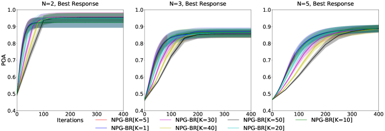
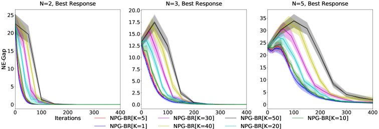
Figure 3: POA (top) and Nash-gap (bottom) under the tabular softmax parameterization (means and standard errors over 10 random initializations).The dashed lines are the curves of the log barrier regularized version of the algorithms with the same color.

H.2 Effect of the log barrier coefficient $\lambda$ for the PG dynamics under tabular softmax

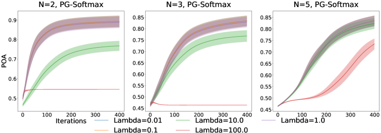
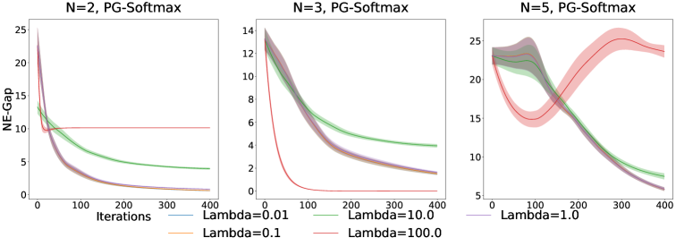
Figure 4: POA (top) and Nash-gap (bottom) for the PG dynamics under the tabular softmax parameterization (means and standard errors over 10 random initializations) with various choices for $\lambda$, the log barrier regularization coefficient.

In Figure 1, we plot in the dashed lines the best-performing $\lambda$, the log barrier regularization coefficient, for the PG dynamics under tabular softmax. Figure 4 complement the results with the POA and Nash-gap curves with various choices for $\lambda$ we searched.

References

- Agarwal et al. (2019) Agarwal, A., Kakade, S. M., Lee, J. D., and Mahajan, G. On the theory of policy gradient methods: Optimality, approximation, and distribution shift. arXiv preprint arXiv:1908.00261, 2019.
- Callaway & Hiskens (2010) Callaway, D. S. and Hiskens, I. A. Achieving controllability of electric loads. Proceedings of the IEEE, 99(1):184–199, 2010.
- Chu et al. (2019) Chu, T., Wang, J., Codecà, L., and Li, Z. Multi-agent deep reinforcement learning for large-scale traffic signal control. IEEE Transactions on Intelligent Transportation Systems, 21(3):1086–1095, 2019.
- Corke et al. (2005) Corke, P., Peterson, R., and Rus, D. Networked robots: Flying robot navigation using a sensor net. In Robotics research. The eleventh international symposium, pp. 234–243. Springer, 2005.
- Foerster et al. (2017) Foerster, J., Farquhar, G., Afouras, T., Nardelli, N., and Whiteson, S. Counterfactual multi-agent policy gradients. arXiv preprint arXiv:1705.08926, 2017.
- Fox et al. (2022) Fox, R., Mcaleer, S. M., Overman, W., and Panageas, I. Independent natural policy gradient always converges in markov potential games. In International Conference on Artificial Intelligence and Statistics, pp. 4414–4425. PMLR, 2022.
- Hu & Wellman (2003) Hu, J. and Wellman, M. P. Nash q-learning for general-sum stochastic games. Journal of machine learning research, 4(Nov):1039–1069, 2003.
- Leonardos et al. (2021) Leonardos, S., Overman, W., Panageas, I., and Piliouras, G. Global convergence of multi-agent policy gradient in markov potential games. arXiv preprint arXiv:2106.01969, 2021.
- Li et al. (2021) Li, G., Wei, Y., Chi, Y., Gu, Y., and Chen, Y. Softmax policy gradient methods can take exponential time to converge. In Conference on Learning Theory, pp. 3107–3110. PMLR, 2021.
- Lowe et al. (2017) Lowe, R., Wu, Y. I., Tamar, A., Harb, J., Abbeel, O. P., and Mordatch, I. Multi-agent actor-critic for mixed cooperative-competitive environments. In Advances in neural information processing systems, pp. 6379–6390, 2017.
- Macua et al. (2018) Macua, S. V., Zazo, J., and Zazo, S. Learning parametric closed-loop policies for markov potential games. arXiv preprint arXiv:1802.00899, 2018.
- Mei et al. (2020) Mei, J., Xiao, C., Szepesvari, C., and Schuurmans, D. On the global convergence rates of softmax policy gradient methods. In International Conference on Machine Learning, pp. 6820–6829. PMLR, 2020.
- Mirrokni & Vetta (2004) Mirrokni, V. S. and Vetta, A. Convergence issues in competitive games. In Approximation, randomization, and combinatorial optimization. algorithms and techniques, pp. 183–194. Springer, 2004.
- Roughgarden (2015) Roughgarden, T. Intrinsic robustness of the price of anarchy. Journal of the ACM (JACM), 62(5):1–42, 2015.
- Roughgarden (2016) Roughgarden, T. Twenty lectures on algorithmic game theory. Cambridge University Press, 2016.
- Shapley (1953) Shapley, L. S. Stochastic games. Proceedings of the national academy of sciences, 39(10):1095–1100, 1953.
- Tesauro (2003) Tesauro, G. Extending q-learning to general adaptive multi-agent systems. Advances in neural information processing systems, 16, 2003.
- Zhang et al. (2018) Zhang, K., Yang, Z., Liu, H., Zhang, T., and Başar, T. Fully decentralized multi-agent reinforcement learning with networked agents. arXiv preprint arXiv:1802.08757, 2018.
- Zhang et al. (2020) Zhang, K., Kakade, S., Basar, T., and Yang, L. Model-based multi-agent rl in zero-sum markov games with near-optimal sample complexity. Advances in Neural Information Processing Systems, 33:1166–1178, 2020.
- Zhang et al. (2021) Zhang, R., Ren, Z., and Li, N. Gradient play in stochastic games: stationary points, convergence, and sample complexity. arXiv preprint arXiv:2106.00198, 2021.