Abstract

While the optimal transport (OT) problem was originally formulated as a linear program, the addition of entropic regularization has proven beneficial both computationally and statistically, for many applications. The Sinkhorn fixed-point algorithm is the most popular approach to solve this regularized problem, and, as a result, multiple attempts have been made to reduce its runtime using, e.g., annealing in the regularization parameter, momentum or acceleration. The premise of this work is that initialization of the Sinkhorn algorithm has received comparatively little attention, possibly due to two preconceptions: since the regularized OT problem is convex, it may not be worth crafting a good initialization, since any is guaranteed to work; secondly, because the outputs of the Sinkhorn algorithm are often unrolled in end-to-end pipelines, a data-dependent initialization would bias Jacobian computations. We challenge this conventional wisdom, and show that data-dependent initializers result in dramatic speed-ups, with no effect on differentiability as long as implicit differentiation is used. Our initializations rely on closed-forms for exact or approximate OT solutions that are known in the 1D, Gaussian or GMM settings. They can be used with minimal tuning, and result in consistent speed-ups for a wide variety of OT problems.

1 Introduction

The optimal assignment problem and its generalization, the optimal transport (OT) problem, play an increasingly important role in modern machine learning. These problems define the Wasserstein geometry (Santambrogio,, 2015; Peyré et al.,, 2019), which is routinely used as a loss function in imaging (Schmitz et al.,, 2018; Janati et al.,, 2020), but also used to reconstruct correspondences between datasets, as for instance in domain adaptation (Courty et al.,, 2014, 2017) or single-cell genomics (Schiebinger et al.,, 2019). Several recent applications use OT to obtain an intermediate representation, as in self-supervised learning (Caron et al.,, 2020), balanced attention (Sander et al.,, 2022), parameterized matching (Sarlin et al.,, 2020), differentiable sorting and ranking (Adams and Zemel,, 2011; Cuturi et al.,, 2019, 2020; Xie et al., 2020a, ), differentiable resampling (Corenflos et al.,, 2021) and clustering (Genevay et al.,, 2019).

Sinkhorn as a subroutine for OT. A striking feature of all of the approaches outlined above is that they do not rely on the linear programming formulation of OT (Ahuja et al.,, 1988, §9-11), but use instead an entropy regularized formulation (Cuturi,, 2013). This formulation is typically solved with the  Sinkhorn, algorithm (1967), which has gained popularity for its versatility, efficiency and differentiability.

Ever Faster Sinkhorn. Given two discrete measures, the Sinkhorn algorithm runs a fixed-point iteration that outputs two optimal dual vectors, along with their objective–a proxy for their Wasserstein distance. Because Sinkhorn is often used as an inner routine within more complex architectures, its contribution to the total runtime may result in a substantial share of the entire computational burden. As a result, accelerating the Sinkhorn algorithm is crucial, and has been explored along two lines of works: through faster kernel matrix-vector multiplications, using geometric properties (Solomon et al.,, 2015; Altschuler et al.,, 2019; Scetbon and Cuturi,, 2020), or by reducing the total number of iterations needed to converge, using e.g. an annealing regularization parameter (Kosowsky and Yuille,, 1994; Schmitzer,, 2019; Xie et al., 2020b, ), momentum (Thibault et al.,, 2021; Lehmann et al.,, 2021), or Anderson, acceleration (1965), as considered in (Chizat et al.,, 2020).

Initialization as a Blind Spot. All methods above are, however, implemented by default by setting initial dual vectors naively at $\mathbf{0}$.

To our knowledge, initialization schemes have only been explored in a few restricted setups, such as semi-discrete settings in 2/3D (Meyron,, 2019), or for discrete Wasserstein barycenter problems (Cuturi and Peyré,, 2015). We argue that careful initialization of dual potentials presents an overlooked opportunity for efficiency.

Contributions. We propose multiple methods to initialize dual vectors. Contrary to concurrent and complementary work by Amos et al., (2022), our initializers are not trained, and not limited to fixed support setups. They require minimal hyperparameter tuning and result in small to negligible overheads. To do so, we leverage closed-form formulae and approximate solutions for simpler OT problems, resulting in the following procedures:

• We introduce a method to recover dual vectors when the primal problem solution is known in closed-form, and apply this to the non-regularized 1D problem. We show that initializing Sinkhorn with these vectors results in orders of magnitude speedups that can be readily applied to differentiable sorting and ranking.

• When the ground cost is the squared L2 distance in $\mathbb{R}^{d}$, $d>1$, we leverage closed-form dual potential functions from the Gaussian approximation of source/target measures, and evaluate them on source points to initialize the Sinkhorn algorithm. We extend this by introducing an approximation of OT potentials for Gaussian mixtures.

• Finally we reformulate the multiscale approach of (Feydy,, 2020, Alg. 3.6) as a subsample initializer.

We provide extensive empirical evaluation, and compare our approaches to other acceleration methods. We show that our initializations are robust and effective, outperforming existing alternatives, yet can also work in combination with them to achieve even better results.

2 Background material on OT

2.1 Entropic Regularization and Sinkhorn

Given two discrete probability measures $\mu=\sum_{i=1}^{n}a_{i}\delta_{x_{i}}$ and $\nu=\sum_{j=1}^{m}b_{j}\delta_{y_{j}}$ in $\mathcal{P}(\mathbb{R}^{d})$, where ${\mathbf{a}=(a_{1},\dots,a_{n})}$, ${\mathbf{b}=(b_{1},\dots,b_{m})}$ are probability weights and ${(\mathbf{x}_{1},\dots,\mathbf{x}_{n})\in\mathbb{R}^{d\times n}}$, ${(\mathbf{y}_{1},\dots,\mathbf{y}_{m})\in\mathbb{R}^{d\times m}}$, the entropy regularized OT problem between $\mu$ and $\nu$ parameterized by $\varepsilon\geq 0$ and a cost function $c$ has two equivalent formulations,

$$\min_{\begin{subarray}{c}\mathbf{P}\in\mathbb{R}_{+}^{n\times m},\mathbf{P}\mathbf{1}_{m}=\mathbf{a},\mathbf{P}^{T}\mathbf{1}_{n}=\mathbf{b}\end{subarray}}\!\!\!\langle\mathbf{P},\mathbf{C}\rangle-\varepsilon\langle\mathbf{P},\log(\mathbf{P})-1\rangle\,,$$ (1)

$$\!\!\!\!\!\!\max_{\mathbf{f}\in\mathbb{R}^{n},\mathbf{g}\in\mathbb{R}^{m}}\!\!\!\!\mathcal{E}_{\mu,\nu,c,\varepsilon}(\mathbf{f},\mathbf{g})\!:=\!\langle\mathbf{f},\mathbf{a}\rangle\!+\!\langle\mathbf{g},\mathbf{b}\rangle-\!\varepsilon\langle e^{\tfrac{\mathbf{f}}{\varepsilon}},\mathbf{K}e^{\tfrac{\mathbf{g}}{\varepsilon}}\rangle.\!$$ (2)

where $\mathbf{C}:=[c(\mathbf{x}_{i},\mathbf{y}_{j})]_{i,j}$, with corresponding kernel $\mathbf{K}:=e^{-\mathbf{C}/\varepsilon}$. While $(\mathbf{f},\mathbf{g})$ are unconstrained for $\varepsilon>0$, the regularization term converges as $\varepsilon\rightarrow 0$ to an indicator function that requires $\mathbf{f}_{i}+\mathbf{g}_{j}\leq c(\mathbf{x}_{i},\mathbf{y}_{j})$.

1:  Input: $\mathbf{a},\mathbf{b},\mathbf{C},\varepsilon>0,\omega>0,\mathbf{f}^{(0)},\mathbf{g}^{(0)}$.

2:  Initialize: $\mathbf{f}\leftarrow\mathbf{f}^{(0)},\mathbf{g}\leftarrow\mathbf{g}^{(0)}$

3:  while not converged do

4:     $\mathbf{f}\leftarrow\omega(\varepsilon\log\mathbf{a}-\min_{\varepsilon}(\mathbf{C}-\mathbf{f}\oplus\mathbf{g}))+\mathbf{f}$

5:     $\mathbf{g}\leftarrow\omega(\varepsilon\log\mathbf{b}-\min_{\varepsilon}(\mathbf{C}^{T}-\mathbf{g}\oplus\mathbf{f}))+\mathbf{g}$

6:  end while

7:  Return $\mathbf{f},\mathbf{g}$

Algorithm 1 Sinkhorn’s Algorithm

The Sinkhorn Algorithm. Algorithm 1 describes a sequence of updates to optimize $\mathbf{f},\mathbf{g}$ in (2). When $\omega=1$, these updates correspond to cancelling alternatively the gradients $\nabla_{1}\mathcal{E}_{\mu,\nu,c,\varepsilon}(\mathbf{f},\mathbf{g})$ (line 4) and $\nabla_{2}\mathcal{E}_{\mu,\nu,c,\varepsilon}(\mathbf{f},\mathbf{g})$ (line 5) of the objective in (2). These updates use the row-wise soft-min operator $\min_{\varepsilon}$, defined as:

$$\text{Given }\mathbf{S}=[\mathbf{S}_{i,j}],\,\text{min}_{\varepsilon}(\mathbf{S}):=[-\varepsilon\log\left(\mathbf{1}^{T}e^{-\mathbf{S}_{i,\cdot}/\varepsilon}\right)]_{i}\,,$$

and the tensor addition notation $\mathbf{f}\oplus\mathbf{g}=[\mathbf{f}_{i}+\mathbf{g}_{j}]_{i,j}$. The runtime of the Sinkhorn algorithm hinges on several factors, notably the choice of $\varepsilon$. Several works report that hundreds of iterations are typically required when using fairly small regularization $\varepsilon$ (e.g. 500 in Salimans et al., 2018, App.B). These scalability issues are compounded in advanced applications whereby multiple Sinkhorn layers are embedded in a single computation or batched across examples (Cuturi et al.,, 2019; Xie et al., 2020a, ; Cuturi et al.,, 2020). To mitigate runtime issues, popular acceleration techniques such as fixed (Thibault et al.,, 2021) or adaptive (Lehmann et al.,, 2021) momentum approaches, as well as Anderson acceleration (Chizat et al.,, 2020) have been considered. While acceleration methods are known to work well when initialized not too far away from optima (d’Aspremont et al.,, 2021), all common implementations (Flamary et al.,, 2021; Cuturi et al.,, 2022) initialize these vectors to $(\mathbf{0}_{n},\mathbf{0}_{m})$.

2.2 Dual Variables in the Sinkhorn Algorithm

On starting closer to the solution. While the Sinkhorn algorithm will converge with any initialization, the speed of convergence is bounded by  (Peyré et al.,, 2019, Rem. 4.14):

$$\|\mathbf{f}^{(\ell)}-\mathbf{f}^{\star}\|_{\text{var}}\leq\|\mathbf{f}^{(0)}-\mathbf{f}^{\star}\|_{\text{var}}\lambda(\mathbf{K})^{2\ell}\,,$$ (3)

where $\mathbf{f}^{(\ell)}$ denotes the potential vector $\mathbf{f}$ obtained after running  Algorithm 1 for $\ell$ iterations, $\mathbf{f}^{\star}$ the optimal potential, and deviation is measured using the variation norm. $\lambda(\mathbf{K})$ reflects conditioning in $\mathbf{K}$ (Peyré et al.,, 2019, Theorem 4.1), determined by the range and magnitude of costs evaluated on $(\mathbf{x}_{i},\mathbf{y}_{j})$ pairs relative to $\varepsilon$. Since $0<\lambda(\mathbf{K})<1$, the Sinkhorn algorithm converges more slowly as $\lambda(\mathbf{K})$ approaches $1$. The motivation to obtain a better initialization relies on targeting the initial gap in $\|\mathbf{f}^{(0)}-\mathbf{f}^{\star}\|_{\text{var}}$.

Two or One Dual Initializations? While Algorithm 1 lists two initial vectors $(\mathbf{f}^{(0)},\mathbf{g}^{(0)})$, a closer inspection of the updates shows that only a single dual variable is needed: when starting with an iteration updating $\mathbf{g}$, only $\mathbf{f}^{(0)}$ is required (the reference to $\mathbf{g}$ is only there for numerical stability). Conversely, only $\mathbf{g}^{(0)}$ is required when updating $\mathbf{f}$. Since only one is needed, we supply by default the smallest vector when $n\neq m$, and set the other to $\mathbf{0}$.

Differentiability and Dual initialization. Any output of the Sinkhorn fixed-point algorithm can be differentiated using unrolling (Adams and Zemel,, 2011; Hashimoto et al.,, 2016; Genevay et al.,, 2018, 2019; Cuturi et al.,, 2019; Caron et al.,, 2020). This approach has, however, two drawbacks: its memory footprint grows as $L(n+m)$, where $L$ is the number of iterations needed to converge, and, more fundamentally, it prevents us from using more efficient steps, such as adaptive momentum and acceleration, because they typically involve non-differentiable operations. These issues can be avoided by relying instead on implicit differentiation (Luise et al.,, 2018; Cuturi et al.,, 2020; Xie et al., 2020b, ; Cuturi et al.,, 2022), which only requires access to solutions $\mathbf{f}^{\star},\mathbf{g}^{\star}$ to work. We recall how this can be implemented for completeness. Introducing the following notations:

$$F: \,\mu,\nu,c,\varepsilon\mapsto\mathbf{f}^{\star},\mathbf{g}^{\star},\text{optimal solutions to\leavevmode\nobreak\ \eqref{eq:erot_d}}\,,$$

$$H: \,\mu,\nu,c,\varepsilon,\mathbf{f},\mathbf{g}\mapsto\begin{bmatrix}\nabla_{1}\mathcal{E}_{\mu,\nu,c,\varepsilon}(\mathbf{f},\mathbf{g})\\ \nabla_{2}\mathcal{E}_{\mu,\nu,c,\varepsilon}(\mathbf{f},\mathbf{g})\end{bmatrix}\,,$$

one has that $H(\mu,\nu,c,\varepsilon,F(\mu,\nu,c,\varepsilon))=\mathbf{0}_{n+m}$, which is the root equation that can be used to instantiate the implicit function theorem, to recover the Jacobian of the outputs of $F$ (i.e. $\mathbf{f}^{\star},\mathbf{g}^{\star}$) w.r.t. any variable “$\blacksquare$” within inputs. As a result, the transpose-Jacobian of $F$ applied to any perturbation of the size of $\blacksquare$ (the only operation needed to implement reverse-mode differentiation) is recovered as (where $\dots$ is a shorthand notation for $\blacksquare,(\mathbf{f}^{\star},\mathbf{g}^{\star})$):

$$J_{F,\blacksquare}(\dots)^{T}z=-J_{H,\blacksquare}(\dots)^{T}\left(J_{H,(\mathbf{f},\mathbf{g})}(\dots)^{T}\right)^{-1}\mathbf{z}$$

All of these operations can be instantiated easily using vjp Jacobian operators (Bradbury et al.,, 2018) and linear systems that rely on linear functions (rather than matrices) as detailed in (Cuturi et al.,, 2022). These computations only require access to optimal values $\mathbf{f}^{\star},\mathbf{g}^{\star}$, not the computational graph that was needed to reach them.

2.3 Closed-Form Expressions in Optimal Transport

A few closed-forms for unregularized ($\varepsilon=0$) OT are known. Some of these closed forms rely on the Monge, formulation of OT, recalled for completeness for two measures $\mu,\nu\in\mathcal{P}(\mathbb{R}^{d})$ in (4), using the push-forward $\sharp$ notation, as well as the dual formulation of OT in (5), using the convention $f^{c}(\mathbf{y}):=\min_{\mathbf{x}}c(\mathbf{x},\mathbf{y})-f(\mathbf{x})$, the $c$-transform of $f$.

$$\min_{\begin{subarray}{c}T:\mathbb{R}^{d}\rightarrow\mathbb{R}^{d}\\ T_{\sharp}\mu=\nu\end{subarray}} \int\!\!c(\mathbf{x},T(\mathbf{x}))\mathrm{d}\mu(\mathbf{x}).$$ (4)

$$\max_{f:\mathbb{R}^{d}\rightarrow\mathbb{R}} \int\!\!f\mathrm{d}\mu+\!\!\int\!\!f^{c}\mathrm{d}\nu\,.$$ (5)

We review two relevant cases, where either an optimal coupling $\mathbf{P}^{\star}$ (for $\varepsilon=0$) in the primal formulation of (1), or an optimal map $T^{\star}$ to (4) can be obtained in closed form. We show in §3 how these solutions can be leveraged to recover initialization vectors $\mathbf{f}^{(0)}$ and $\mathbf{g}^{(0)}$ for Alg. 1.

OT in 1D. For univariate data ($d=1)$, and when the cost function $c$ is such that $-c$ is supermodular $(\partial c/\partial x\partial y<0)$, a solution $\mathbf{P}^{\star}$ to (1) can be recovered in closed form (Chiappori et al.,, 2017; Santambrogio,, 2015, §3). Writing $\sigma$, $\rho$ for sorting permutations of the supports of $\mu$ and $\nu$, $x_{\sigma_{1}}\leq\dots\leq x_{\sigma_{n}}$ and $y_{\rho_{1}}\leq\dots\ y_{\rho_{m}}$, a solution $\mathbf{P}^{\star}$ is given by the north-west corner solution $\textbf{NW}(\mathbf{a}_{\sigma},\mathbf{b}_{\rho})$, where $\mathbf{a}_{\sigma}$ and $\mathbf{b}_{\rho}$ are the weight vectors $\mathbf{a},\mathbf{b}$ permuted using $\sigma$ and $\rho$ respectively (Peyré et al.,, 2019, §3.4.2).

Gaussian. The Monge, formulation of the OT problem (4) from a Gaussian measure $\mathfrak{N}_{1}=\mathcal{N}(\mathbf{m}_{1},\mathbf{\Sigma}_{1}),\mathbf{\Sigma}_{1}>0$, to another $\mathfrak{N}_{2}=\mathcal{N}(\mathbf{m}_{2},\mathbf{\Sigma}_{2})$, is solved by (see also Fig. 1):

$$T^{\star}(\mathbf{x}):=\mathbf{A}(\mathbf{x}-\mathbf{m}_{1})+\mathbf{m}_{2},\mathbf{A}=\mathbf{\Sigma}^{-\frac{1}{2}}_{1}(\mathbf{\Sigma}^{\frac{1}{2}}_{1}\mathbf{\Sigma}_{2}\mathbf{\Sigma}^{\frac{1}{2}}_{1})^{\frac{1}{2}}\mathbf{\Sigma}^{-\frac{1}{2}}_{1}.$$

The optimal dual potential $f^{\star}$ is a quadratic form given by

$$f^{\star}(\mathbf{x})=\tfrac{1}{2}\mathbf{x}^{T}(\mathbf{I}-\mathbf{A})\mathbf{x}+(\mathbf{m}_{2}-\mathbf{A}\mathbf{m}_{1})^{T}\mathbf{x}\,,$$ (6)

which recovers $T^{\star}=\text{Id}-\nabla f^{\star}$. The OT cost between $\mathfrak{N}_{1}$ and $\mathfrak{N}_{2}$ is known as the Bures-Wasserstein distance:

$$W_{2}^{2}(\mathfrak{N}_{1},\mathfrak{N}_{2}) =\|\mathbf{m}_{1}-\mathbf{m}_{2}\|^{2}+\mathcal{B}^{2}_{2}(\Sigma_{1},\Sigma_{2})\,,$$ (7)

$$\mathcal{B}^{2}_{2}(\Sigma_{1},\Sigma_{2}): =\text{tr}(\mathbf{\Sigma}_{1}+\mathbf{\Sigma}_{2}-2(\mathbf{\Sigma}^{\frac{1}{2}}_{1}\mathbf{\Sigma}_{2}\mathbf{\Sigma}^{\frac{1}{2}}_{1})^{\frac{1}{2}})\,.$$

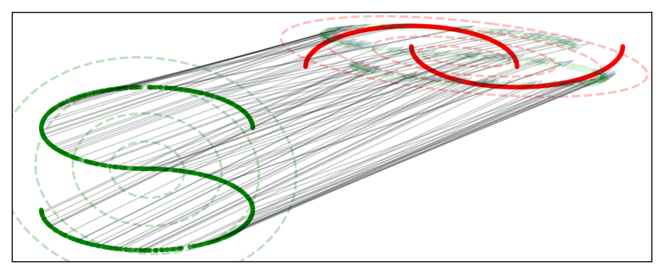
Figure 1: Transport map (black) from Gaussian approximations (dashed) of S-curve (green) and two-moons (red)

3 Crafting Sinkhorn Initializations

We present important scenarios where careful initialization can dramatically speed up the Sinkhorn algorithm. We start with the 1D case (§3.1), where entropic transport has been used recently as a possible approach to obtain differentiable rank and sorting operators. We follow with the generic and by now standard multivariate OT problem in $\mathbb{R}^{d}$ with squared-L2 ground cost, using Gaussian approximations (§3.2) and an extension to mixtures (§3.3).

3.1 Initialization for 1D Regularized OT

Ranking as an OT problem. Using a cost $c$ on $\mathbb{R}\times\mathbb{R}$ such that $\partial c/\partial x\partial y<0$, sorting the entries of a vector $\mathbf{x}=(x_{1},\dots,x_{n})\in\mathbb{R}^{n}$ can be recovered using a solution $\mathbf{P}^{\star}$ to  (1), setting $\varepsilon=0$, $\mathbf{a}=\mathbf{1}_{n}/n$, and $\nu$ to a uniform measure on $n$ increasing numbers, e.g. $\mathbf{y}=(1,2,\ldots,n)$. The ranks of the entries of $\mathbf{x}$ are then $n\mathbf{P}^{\star}\mathbf{z}$, where $\mathbf{z}=(1,2,...,n)$, and its sorted entries as $n\mathbf{P}^{\star T}\mathbf{x}$ (Cuturi et al.,, 2019).

Differentiable Ranking. A differentiable and fractional soft sorting/ranking operator can be derived from entropy regularized couplings, using instead a solution $\mathbf{P}_{\varepsilon}$ to (1, $\varepsilon>0$) to form $n\mathbf{P}_{\varepsilon}\mathbf{z}$ and $n\mathbf{P}_{\varepsilon}^{T}\mathbf{x}$ (Cuturi et al.,, 2019), with the possibility to use a different target size $m$ or non-uniform weights $\mathbf{a},\mathbf{b}$. A practical challenge of that approach is that the number of Sinkhorn iterations needed for the coupling to converge can be typically quite large, see  Figure 3 and further results in  Section B.1.

Dual 1D Initializers. Regularized 1D OT problems often require a small regularization $\varepsilon$ to be meaningful, in order to recover rank approximations that are not too smoothed, which then requires many Sinkhorn iterations to converge. To address this, we introduce an initializer using potentials for the non-regularized problem ($\varepsilon=0$). Our strategy to pick initialization vectors for  Algorithm 1 is upon first glance deceptively simple: sort $\mathbf{x}$, recover a primal solution $\mathbf{P}^{\star}$ (the North-West corner solution) that is guaranteed to solve (1); turn it into a pair of optimal dual vectors $\mathbf{f}^{\star}_{0},\mathbf{g}^{\star}_{0}$ for the same unregularized problem, and seed them to Alg. 1 to solve 2 with $\varepsilon>0$. While obtaining $\mathbf{P}^{\star}$ only requires a sort, efficiently recovering a corresponding dual pair ($\mathbf{f}^{\star}_{0},\mathbf{g}^{\star}_{0}$) is less straightforward. In principle, duals may be obtained by solving an elementary cascading linear system using primal-dual conditions (Peyré et al.,, 2019, §3.5.1). That approach does not always work, however, when the size of the support of $\mathbf{P}^{\star}$ is strictly smaller than $n+m-1$ (it results in a system that has less equalities than variables), which is the case in the original ranking problem, where $n=m$. Sejourne et al., (2022, Alg.1) propose an algorithm to construct $\mathbf{f}^{\star}_{0},\mathbf{g}^{\star}_{0}$ in $n+m$ sequential operations, interlaced with conditional statements. We consider a more generic algorithm that works in higher dimensions, but which, when particularized to the 1D case, results in the DualSort Algorithm 2 (see also Appendix E), a parallel approach with larger $\mathcal{O}(nm)$ complexity, but simpler to deploy on GPU, since it only requires a handful of iterations to converge, each directly comparable to that of the Sinkhorn algorithm. See application to experiments in §4.1 and §4.2.

1:  Input: Cost matrix $\mathbf{C}=[c(x_{\sigma_{i}},y_{\rho_{j}})]$ for the sorted entries of input vectors $\mathbf{x},\mathbf{y}$ entries, see §2.3.

2:  Initialize: $\mathbf{f}=0$

3:  while not converged do

14:     $\mathbf{f}\leftarrow\min_{\text{axis=1}}\left(\mathbf{C}-\textrm{diag}(\mathbf{C})\mathbf{1}^{T}+\mathbf{f}\mathbf{1}^{T}\right)$

5:  end while

6:  Return $\mathbf{f}$

Algorithm 2 DualSort Initializer

3.2 Computing Dual Initializers from Gaussian OT

From optimal potentials to dual initializers. We leverage Gaussian approximations to obtain an efficient initializer, coined Gaus, for the Sinkhorn problem, when $c(x,y)=\|x-y\|^{2}_{2}$, notably when $n\gg d$.

To do so, and given two discrete empirical measures $\mu$ and $\nu$, compute their empirical means and covariance matrices $(\mathbf{m}_{\mu},\mathbf{\Sigma}_{\mu})$ and $(\mathbf{m}_{\nu},\mathbf{\Sigma}_{\nu})$, to recover a dual potential function $f^{\star}$ from  (6) that solves the Gaussian dual OT problem, where $\mathbf{A}$ in that equation can be obtained by replacing $\mathbf{\Sigma}_{1}$ with $\mathbf{\Sigma}_{\mu}$ and $\mathbf{\Sigma}_{2}$ with $\mathbf{\Sigma}_{\nu}$. Next, evaluate that quadratic potential on all observed points of the first measure $[\mathbf{f}^{(0)}]_{i}\leftarrow f^{\star}(\mathbf{x}_{i})$ (or alternatively the second measure if $m<n$) to seed the Sinkhorn algorithm.

Table 1: Toy examples, $n=m=1024$, $d=2$, $200$ runs.

Dataset	# Iterations $(\textrm{mean}\pm\textrm{std})$
	Init $\mathbf{0}$	Init Gaus
2-moons	$120.0\pm 0.0$	$\mathbf{11.0\pm 0.0}$
S curve / 2-moons	$137.2\pm 16.7$	$\mathbf{49.6\pm 14.8}$
3 Gaussian blobs	$236.0\pm 24.3$	$\mathbf{45.4\pm 9.7}$

Complexity. Solving OT on the Gaussian approximations of $\mu,\nu$, requires computing means and covariance matrices $\mathcal{O}((n+m)d^{2})$, as well as matrix square-roots and their inverse, using the Newton-Schulz iterations (Higham,, 2008) at cost $\mathcal{O}(d^{3})$. The Gaus initializer is therefore particularly relevant in settings where $d\ll n$, which is typically the regime where OT has found practical relevance.

Implementation. Our experiments show that Gaus often works significantly better than the default null initialization, notably with toy datasets (see Table  1), but also when computing OT on latent space embeddings as shown in §4.3 and §4.4, or to word-embeddings as demonstrated in §4.5. The overhead induced by the computations of dual solutions is naturally dictated by the tradeoff between $n$ (the number of points) and $d$ (their dimension). In all cases considered here that overhead is negligible, but explored with more care in Appendix C. Note that many of the matrix-squared-roots computations can be pre-stored for efficiency, if the same measure $\mu$ is to be compared repeatedly to other measures.

3.3 Gaussian Mixture Approximations

The Gaussian initialization approach can be extended to Gaussian mixture models (GMMs), resulting in greater flexibility, yet pending further approximations. This requires the additional cost of pre-estimating GMMs for each input measure. By further approximations above, we refer more explicitly to the fact that, unlike for single Gaussians, we do not have access to closed-form OT solutions between GMMs, but instead only “efficient” couplings that return a cost that is an upper-bound on the true Wasserstein distance between two GMMs, as introduced next.

OT in the space of Gaussian measures. Given two Gaussian mixtures $\rho=\sum_{k=1}^{K}\alpha_{k}\rho_{k}$ and $\tau=\sum_{k=1}^{K}\beta_{k}\tau_{k}$, assuming each $\rho_{k}$ and $\tau_{k}$ is itself a Gaussian measure, and that weights $\alpha_{k}$ and $\beta_{k}$ sum to $1$. It was proposed in (Chen et al.,, 2018) to approximate the continuous OT problem between $\rho$ and $\tau$ in the space $\mathbb{R}^{d}$ as a discrete OT problem in the space of mixtures of Gaussians, where each mixture is a discrete measure on $K$ atoms (each atom being a Gaussian), and the ground cost between them is set to the pairwise Bures-Wasserstein distance, forming a cost matrix for (1) as $\mathbf{C}=[W_{2}^{2}(\rho_{i},\tau_{j})]_{ij}$ using (7). That optimization results in two potentials $\tilde{\mathbf{f}}$ and $\tilde{\mathbf{g}}\in\mathbb{R}^{K}$ that solve the corresponding regularized $K\times K$ OT problem.

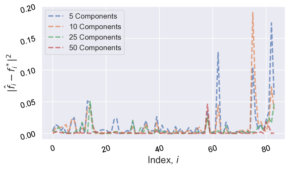
Figure 2: Gap between the true dual $\mathbf{f}^{\star}$ and the GMM approximate dual, for a pair of measures of word embeddings, as a function of $K$, the number of mixture components.

Approximating Dual Potentials with GMMs. Our proposed initializer, GMM, is computed as follows. Given two empirical measures $\mu,\nu$, we fit first two $K$-component GMMs $\tau$ and $\rho$, then obtain two potential vectors $\tilde{\mathbf{f}},\tilde{\mathbf{g}}\in\mathbf{R}^{K}$ using the Sinkhorn algorithm on a $K\times K$ problem, as described above. From those potentials, we propose to compute an approximate $\hat{f}$ dual potential function:

$$\hat{f}(\mathbf{x})=\tilde{\mathbf{f}}^{T}p(\mathbf{x}),\,[\,p(\mathbf{x})]_{k}=\frac{\alpha_{k}d\rho_{k}(\mathbf{x})}{\sum_{l=1}^{K}\alpha_{l}d\rho_{l}(\mathbf{x})}\,.$$ (8)

that is then evaluated on all $n$ points of $\mu$. Intuitively this approximation interpolates continuously the $K$ potentials depending on probability within mixture. This recovers, in the limit where $K\rightarrow n$, $n$ components with means $(x_{i})_{i}$ and zero covariance, resulting in the original potential $\mathbf{f}^{\star}$.

Complexity. Fitting GMMs cost $\mathcal{O}(nKd^{2})$. Computing the Bures-Wasserstein distances between two Gaussian measures would have complexity $\mathcal{O}(d^{3})$ for full covariance matrices and $\mathcal{O}(d)$ for diagonal. Computing the cost matrix for the GMM OT problem would then amount to $\mathcal{O}(K^{2}d^{3})$ or $\mathcal{O}(K^{2}d)$. Since naive Sinkhorn requires $\mathcal{O}(Ln^{2})$ to run between pointclouds of size $n$ for $L$ iterations, and so the proposed GMM initialization may provide, very roughly and not taking into account pre-storage, efficiency gains when $K^{2}d\ll n^{2}$.

3.4 Initialization via Subsampling

We next bring attention to a multi-scale approach described in detail in (Feydy,, 2020, Alg. 3.6), which is a competitive baseline for comparison. Although not how originally described, this approach may be framed as a Sinkhorn initializer which we call the Subsample initializer. The Subsample initializer builds on the idea of the out-of-sample extrapolated entropic potentials (Pooladian and Niles-Weed,, 2021) that are derived readily from a first resolution of the OT problem on a subset of points. Let $\breve{\mu}$, $\breve{\nu}$ denote uniformly subsampled measures of $\mu$ and $\nu$ of size $\breve{n}\ll n$ and $\breve{m}\ll m$. Write $\breve{\mu}=\tfrac{1}{\breve{n}}\sum_{i}\delta_{w_{i}}$, $\breve{\nu}=\tfrac{1}{\breve{m}}\sum_{i}\delta_{z_{i}}$ and write $\breve{\mathbf{f}},\breve{\mathbf{g}}$ the optimal vector dual potentials obtained for (2) for the same regularization $\varepsilon$ and cost, but using $\breve{\mu}$ and $\breve{\nu}$ instead. An initializer for $\mathbf{f}^{(0)}$, can be then defined by using the entropic potential function derived from $\breve{\mathbf{g}}$ (or, alternatively from $\breve{\mathbf{f}}$ if $n\ll m$):

$$[\mathbf{f}^{(0)}]_{i}=\breve{f}(\mathbf{x}_{i}),\text{with}\,\breve{f}:\mathbf{x}\mapsto-\varepsilon\log\tfrac{1}{\breve{m}}\!\sum_{j=1}^{\breve{m}}e^{\frac{\breve{\mathbf{g}}_{j}-c(\mathbf{x}_{,}\mathbf{z}_{j})}{\varepsilon}}.$$ (9)

Although more general than the GMM initializer, the Subsample initializer requires running Sinkhorn on a subsample of points $\breve{n},\breve{m}$ that is typically larger than the $K\times K$ problem induced by $K$-components GMMs. While this may show in runtime costs, as in Figure 7, the Sinkhorn initializer, on the other hand, not affected by large dimensions.

4 Experiments

In this section we illustrate the benefits of our proposed initialization strategies. In particular, we apply DualSort for differentiable sorting and soft-$0/1$ loss from (Cuturi et al.,, 2019). We investigate Gaussian (Gaus) initializers for deep differentiable clustering from (Genevay et al.,, 2019) and differentiable particle filtering from (Corenflos et al.,, 2021). Finally, we showcase GMM initializers with a document similarity task. The purpose of these experiments is to show the benefit of the initializer and not the performance in the particular task, or in claiming these tasks are original. With that in mind, we have not performed extensive network parameter tuning, though we do include some performance metrics to illustrate that the setups are reasonable. Further experimental details are given in Appendix B. Experiments were carried out using OTT-JAX (Cuturi et al.,, 2022), notably acceleration methods for comparison, but also, when relevant, implicit differentiation of Sinkhorn’s outputs.

We compare our proposed approaches to the default $\mathbf{0}$ initialization typical in most Sinkhorn implementations, in addition to fixed  (Thibault et al.,, 2021) and adaptive (Lehmann et al.,, 2021) momentum, $\varepsilon-decay$, as well as Anderson acceleration (Chizat et al.,, 2020).

4.1 Differentiable Sorting

Arrays of size ${n\in\{16,32,64,128,256,512,1024\}}$ were sampled in this experiment from the Gaussian blob dataset (Pedregosa et al.,, 2011) for $200$ different seeds. For each seed, $1$-dimensional Gaussian data was generated from $5$ random centers with centers uniformly distributed in $(-10,10)$ with standard deviation $3$. The Sinkhorn algorithm was then ran with the proposed initialization, DualSort, and with the default zero initializer, labelled $\mathbf{0}$. Other Sinkhorn acceleration methods were also investigated including Anderson acceleration (And$=5$), momentum ($\text{mom.}=1.05$), regularization decay ($\varepsilon\textrm{ decay}=0.8$) and adaptive momentum (adapt$=10$, meaning adaptation is recomputed after 10 iterations). The parameter values for these competing methods were pre-tuned following an initial hyper-parameter sweep.

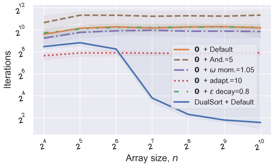
Figure 3: DualSort with a default Sinkhorn setup dominates all existing acceleration methods implemented when run with a default $\mathbf{0}$ initialization. We plot median, upper and lower quartiles of iterations needed to converge over $200$ seeds for various array sizes (iterations for DualSort include steps for the primal-dual procedure).

Figures 3 and 4 illustrate the dramatic speed-up effect from using the DualSort procedure, with just $3$ vectorized iterations. Figure 3 compares Sinkhorn algorithm with initialization to Sinkhorn enhanced through other acceleration method. Figure 4 illustrates the relative-speed up from including initialization along with other enhancements where speed-up is defined as the ratio of iterations using the zero initializer and the DualSort initializer, hence $>1$ indicates an improvement using DualSort. DualSort complements existing acceleration methods. When the DualSort initializer is paired with other acceleration methods, we still observe, no matter which one is used, very large speedups.

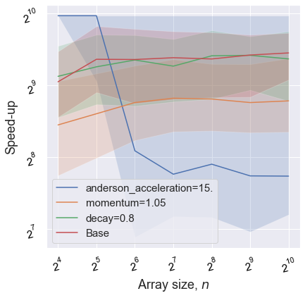
Figure 4: Relative speed-up (higher is better). Median, upper and lower quartiles of iterations needed to converge over $200$ seeds for various array sizes (iterations for DualSort include steps for the primal-dual procedure).

Runtime cost. The DualSort initializer’s runtime cost is negligible and took just $0.0012$ seconds (s) to run for all experiments. The resulting absolute speed-up was $0.06s$ to $0.13$s per OT problem. See further timing details in Appendices B.1. Note that this speed-up is compounded when running many thousands of OT problems.

Table 2: Average time in seconds for DualSort with 3 iterations and Sinkhorn iterations to convergence over 200 soft sorting problems for Gaussian blob data of dimension $n$

$n$	Initializer	Initialization	Iterations
$32$	$\mathbf{0}$	-	$0.28$
	DualSort	$0.0012$	$0.22$
$64$	$\mathbf{0}$	-	$0.22$
	DualSort	$0.0012$	$0.088$
$128$	$\mathbf{0}$	-	$0.17$
	DualSort	$0.0012$	$0.066$
$256$	$\mathbf{0}$	-	$0.17$
	DualSort	$0.0012$	$0.049$
$512$	$\mathbf{0}$	-	$0.13$
	DualSort	$0.0012$	$0.050$
$1024$	$\mathbf{0}$	-	$0.14$
	DualSort	$0.0012$	$0.058$

4.2 Soft Error Classification

The following experiment demonstrates the differentiability of the soft-sorting and ranking operations as well as how the DualSort initializer improves computational performance for real tasks.

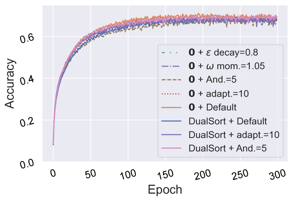
Figure 5: Accuracy of CNN classifier by Sinkhorn methods for CIFAR-100 with soft-error loss and $\varepsilon=0.01$

Let ${h_{\theta}:\mathcal{X}\rightarrow\mathbb{R}^{K}}$ be a parameterized $K$-label classifier and $R$ the differentiable ranking operator described in §3.1. For input $x\in\mathcal{X}$, the soft-$0/1$ loss (or soft-error) evaluated at labeled $(x,y)$, $y\leq K$, is therefore $\max(0,K-R(h_{\theta}(x))_{y})$, see (Cuturi et al.,, 2019) for details.

Table 3: Soft-Error: CIFAR 100, mean $\pm$ std of Sinkhorn iter./ training step, over $10$ seeds

	Iterations	Runtime ($\times 10^{-2}$s)
Zero	$17.9\pm 0.1$	$8.23\pm 0.2$
Anderson	$12.3\pm 0.2$	$5.74\pm 0.2$
Momentum	$15.7\pm 0.2$	$7.70\pm 0.2$
Adaptive	$15.2\pm 0.2$	$7.38\pm 0.3$
$\varepsilon$-decay	$17.0\pm 0.1$	$7.99\pm 0.2$
DualSort	${9.7\pm 0.1}$	$5.07\pm 0.3$
DualSort, Adap.	${10.3\pm 0.1}$	$5.27\pm 0.3$
DualSort, Ande.	$\mathbf{8.2\pm 0.1}$	$\mathbf{3.72\pm 0.3}$

We follow the experimental setup from (Cuturi et al.,, 2019). The classifier network from (Cuturi et al.,, 2022) is used for CIFAR-100, consisting of four CNN layers, and a fully connected hidden layer, full details given in §B.2.

The $\varepsilon$ regularization was set to $0.01$ and the network was trained until convergence over $10$ seeds. DualSort initializer was ran with $3$ iterations, which, as discussed in §3.1, is slightly cheaper than two Sinkhorn iterations.

Accuracy on the evaluation set is shown in Figure 5 for $300$ epochs. It is clear that, as expected, the Sinkhorn initialization procedure does not affect training nor accuracy. However, Table 3 shows that the DualSort initializer drastically reduces the number of Sinkhorn iterations needed for convergence, to compute the soft-error loss and its gradients at each evaluation.

4.3 Differentiable Clustering

We demonstrate the performance improvement from the Gaussian initializer on the task of deep differentiable clustering, with the experimental setup of (Genevay et al.,, 2018). Differentiable clustering aims at producing a latent representation amenable to clustering. This is achieved using a variational autoencoder (Kingma et al.,, 2014) with learnable, discrete cluster embeddings, and an additional loss term allocating encodings to cluster embeddings using OT.

Table 4: Avg. Sinkhorn iter./training step and runtime / training step $\textrm{mean}\pm\textrm{std}$ for differentiable clustering VAE, $10$ seeds, $\epsilon=0.001$

	Iterations	Runtime ($\times 10^{-3}$ s)
Zero	$354.1\pm 7.0$	${25.4\pm 0.2}$
$\varepsilon$-decay	${340.5\pm 17.8}$	${25.1\pm 0.1}$
Anderson	${844.4\pm 26.2}$	${144\pm 6.7}$
Momentum	${342.5\pm 3.7}$	${33.1\pm 1.7}$
Adaptive	${96.6\pm 4.1}$	${9.35\pm 0.02}$
Gaus	${196.6\pm 6.7}$	${16.2\pm 0.6}$
Gaus, Adapt.	$\mathbf{68.7\pm 1.3}$	$\mathbf{8.00\pm 0.1}$

For data of dimension $d_{x}$ and latent dimension $d_{z}$, let $E_{\theta}:\mathbb{R}^{d_{x}}\rightarrow\mathbb{R}^{2\times d_{z}}$ and $D_{\theta}:\mathbb{R}^{d_{z}}\rightarrow\mathbb{R}^{d_{x}}$ denote an encoder and decoder respectively, parameterized by $\theta$. Let $\mu_{\phi}\in\mathbb{R}^{K\times d_{z}}$ denote cluster embeddings for $K$ clusters. The objective of differentiable clustering is to learn $E_{\theta},D_{\theta}$ and embeddings $\mu_{\phi}\in\mathbb{R}^{K\times d_{z}}$. This may be achieved by minimizing the loss $\ell^{\textrm{ae}}(\theta)+\ell^{\textrm{OT}}(\phi,\theta)$ for each batch of data $(x_{i})_{i}$. Here $\ell^{\textrm{ae}}(\theta)$ is the standard variational auto-encoder loss and $\ell^{\textrm{OT}}(\phi,\theta)$ is the regularized OT loss from (1) between $\mu=\sum_{k=1}^{K}\tfrac{1}{K}\delta_{\mu_{\phi k}}$ and $\nu=\sum_{i=1}^{n}\tfrac{1}{n}\delta_{z_{i}}$. $z_{i}=\mathbf{m}_{i}+\sigma_{i}u_{i}$, where $(\mathbf{m}_{i},\sigma_{i})=E_{\theta}(x_{i})$, $u_{i}\sim\mathcal{N}(\mathbf{0}_{d_{z}},\mathbf{I}_{d_{z}})$, and $\tilde{x}_{i}=D_{\theta}(z_{i})$.

We demonstrate this task for MNIST (Deng,, 2012) over $10$ seeds. Fully connected networks with $4$ hidden layers were used for $E_{\theta}$ and $D_{\theta}$, where $d_{z}=32$ and $d_{x}=784$, further experimental details are given in §B.3. Table 4 shows that the Gaussian initializer outperforms the zero initialization for default Sinkhorn and all other combinations of default Sinkhorn plus acceleration techniques. Performance metrics and samples from the generative model are given in Appendix B.3.

4.4 Differentiable Particle Filtering

As introduced in Corenflos et al., (2021), the Sinkhorn algorithm provides an approximate differentiable resampling scheme, hence enables end-to-end differentiable particle filtering. Consider a simple linear state space model consisting of latent states $x_{t}\in\mathbb{R}^{2}$ where $x_{0}=\mathbf{0}$, $X_{t}|x_{t-1}\sim f(\cdot|x_{t-1})=\mathcal{N}(0.5\mathbb{I}x_{t-1},\mathbb{I})$ and observations $y_{t}\in\mathbb{R}^{2}$, $y_{t}\sim g(\cdot|x_{t})=\mathcal{N}(x_{t},\mathbb{I})$ for $t\in\{1,\ldots,T\}$, and time series length $T=500$. Differentiable resampling via OT consists of applying the Sinkhorn algorithm between weighted and unweighted pointclouds of $N$ simulated latent states at each timepoint $t$, for each forward pass. For full details see Corenflos et al., (2021).

Table 5: Mean $\pm$ std number of Sinkhorn iterations and runtime over $3$ seeds for the forward pass of a particle filter with $N$ particles, batch size $4$ of simple linear state space model, $T=500$.

N	Initializer	Iterations (’000s)	Runtime /s
$32$	Gaus	$440\pm 2.5$	$12.08\pm 0.25$
	$\mathbf{0}$	$611\pm 3.4$	$15.46\pm 0.35$
$64$	Gaus	$349\pm 2.9$	$9.62\pm 1.29$
	$\mathbf{0}$	$532\pm 3.4$	$12.49\pm 0.69$
$128$	Gaus	$269\pm 0.7$	$7.03\pm 1.21$
	$\mathbf{0}$	$471\pm 2.3$	$10.18\pm 0.88$
$256$	Gaus	$216\pm 1.5$	$6.340.78$
	$\mathbf{0}$	$439\pm 1.9$	$11.01\pm 0.59$
$512$	Gaus	$176\pm 1.3$	$14.43\pm 1.40$
	$\mathbf{0}$	$422\pm 1.7$	$30.17\pm 1.06$

For batch size $B=4$ and time steps $T=500$, under a naive implementation, each forward pass requires $T\times B$ Sinkhorn layer evaluations. This can be slow. As shown in Table 5, the Gaussian initializer is effective at reducing the runtime by reducing the number of Sinkhorn iterations by approximately $33\%$ to $50\%$ relative to the default Sinkhorn with $\mathbf{0}$ initialization.

4.5 Document Similarity

In this experiment, we compare the Gaus, GMM and Subsample initializers. Documents were gathered from the $20$ Newsgroup dataset (Lang,, 1995) and each word, $(w_{i})_{i=1}^{n}$, in the vocabulary across documents is embedded using the pre-trained GloVe word embeddings (Pennington et al.,, 2014) as $(e_{i})_{i=1}^{n}$ where $e_{i}\in\mathbb{R}^{50}$.

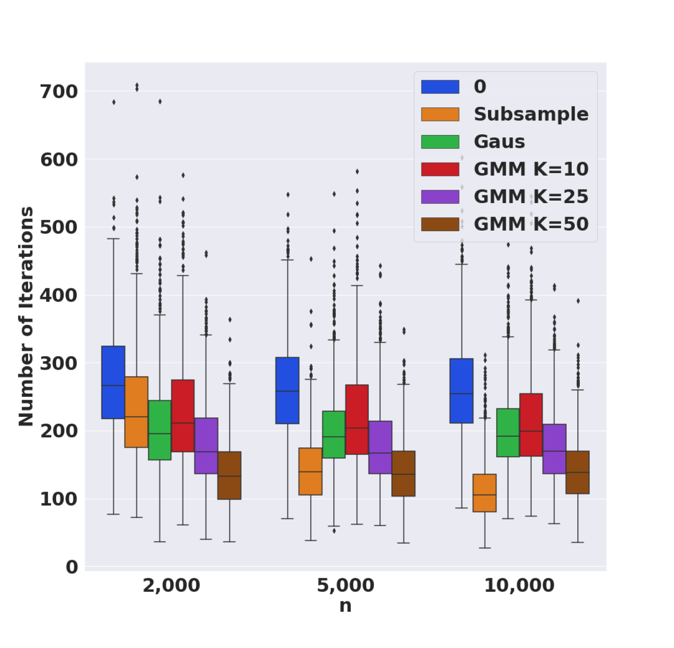
Figure 6: Distribution of number of Sinkhorn iterations required for Sinkhorn convergence between 1225 pairs of Newsgroup documents, represented as word embeddings histograms, $n$ being the total vocabulary size. The same convergence threshold for Sinkhorn is used for all $n$.

In a similar setup to Kusner et al., (2015), each document may be represented as a histogram with weights $(a_{i})_{i=1}^{n}$ corresponding to word-frequency, $\nu_{i}=\sum_{i=1}^{n}a_{i}\delta_{e_{i}}$, and we compute pairwise OT distances between $50$ documents, resulting in $1,225$ pairs. We report the number of Sinkhorn iterations and runtime required for convergence for the default zero intializer ($\mathbf{0}$), the proposed Gaus initializer, the GMM initializers with full covariance matrices and $K\in\{10,25,50\}$ components, and the Subsample initializer. A subset of the vocabulary of size $n\in\{2\times 10^{3},5\times 10^{3},10^{4}\}$ was used, and corresponding subsample of size $100,500$ and $1,000$ for the Subsample initializer. Regularization was $\varepsilon=0.001$.

The distribution of results are shown in Figure 6 and Figure 7 illustrating that improvements can be obtained for a range of $K$. Notice however that Gaus beats the GMM for low $K$, we suspect this is due to the additional approximation (8). Although often resulting in lower number of fine-tuning Sinkhorn iterations, the preprocessing cost of running the Subsample initializer is expensive, and only exhibits better aggregate runtime performance for large $n=10,000$, which was expected. A GMM was first fitted to each document, before being used for initializing Sinkhorn potentials. As Figure 7 shows, although the cost of fitting GMMs results in limited runtime savings for $n=2,000$, there are significant runtime savings for $n=5,000$ and $n=10,000$. See further discussion in §C.

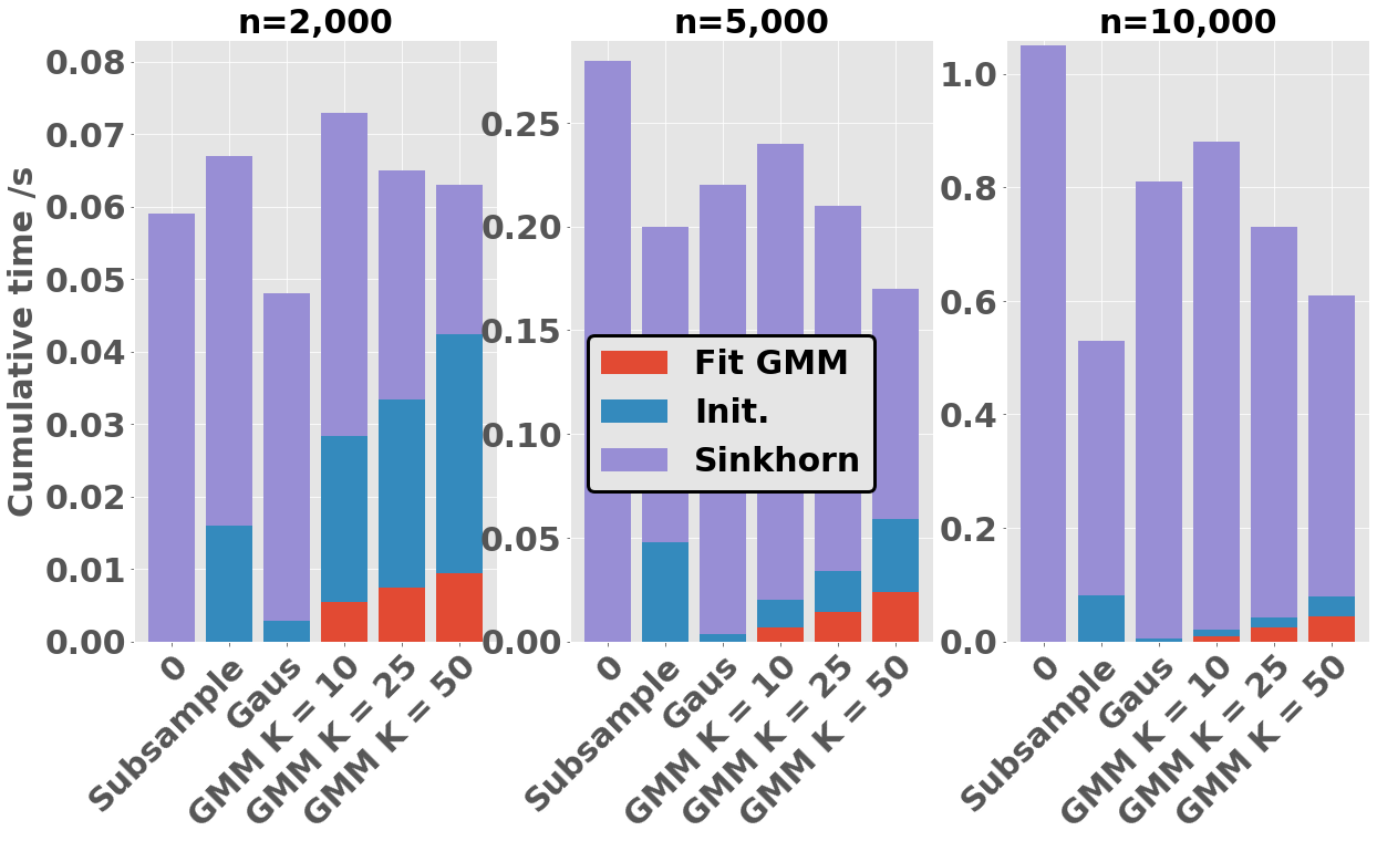
Figure 7: Average wall clock time for computing OT between each pair of word-embeddings ($1,225$ problems) for vocabulary of size $n=2\times 10^{3};5\times 10^{3};10^{4}$; split by initialization time (Init), time to compute Gaussian mixture models (Fit GMM) and Sinkhorn iterations (Sinkhorn).

5 Conclusion

We have introduced efficient and robust Sinkhorn potential initialization schemes: DualSort, Gaus, GMM and demonstrated how these carefully chosen initializers can significantly improve the performance of the Sinkhorn algorithm for a variety of tasks. These GPU-friendly initializers may also be embedded in end-to-end differentiable procedures by relying on implicit differentiation, as demonstrated in various tasks presented in our experiments (ranking, clustering, filtering), and are complementary to most common acceleration methods, creating an interesting space to optimize further the execution of Sinkhorn. Initialization is a neglected area of computational OT, and we hope that these promising results can inspire new research to other areas, such as initalizing calls to Sinkhorn in the internal loops of the Gromov-Wasserstein or barycenter problem. We also hope they can help extending OT’s reach to data-hungry application areas, such as single-cell or NLP tasks that involve typically a large number of samples.

Appendix A Dual Potential Comparison

For balanced OT problems, as considered here, Dual potentials $\mathbf{f}$, $\mathbf{g}$ are unique up to constant shifts i.e. $\mathbf{f}-s$, $\mathbf{g}+s$ for $s\in\mathbb{R}$. Therefore, in order to compare potentials $\mathbf{f}\in\mathbb{R}^{n}$, we center $\mathbf{f}$, as $\mathbf{f}\leftarrow\mathbf{f}-\frac{1}{n}\sum_{i}\mathbf{f}_{i}$.

A.1 From Optimal Primal to Dual Vectors

Properties of the optimal primal $\mathbf{P}^{\star}$. Taking the 1D case as motivation, we introduce a method to recover optimal dual potentials $\mathbf{f^{\star},g^{\star}}$ from an optimal primal solution $\mathbf{P}^{\star}$. To that end, one can cast an OT problem as a min-cost-flow problem on a bipartite graph $\mathcal{G}=(\mathcal{V},\mathcal{E})$, with vertices composed of source nodes $S=\{1,\ldots,n\}$ and target nodes $T=\{1^{\prime},\ldots,m^{\prime}\}$, $\mathcal{V}=S\cup T$, and edge set $\mathcal{E}=\{(i,j^{\prime}),i=1,\dots,n;j=1,\dots,m\}$ linking them. The KKT conditions state that, writing $\mathcal{E}(\mathbf{P})=\{(i,j^{\prime})|\mathbf{P}_{i,j}>0\}$ one has that the graph $(\mathcal{V},\mathcal{E}(\mathbf{P}^{\star}))$ is necessarily a forest (Peyré et al.,, 2019, Prop. 3.4).

We write $\mathcal{T}_{1},\dots,\mathcal{T}_{K}$ for the $K$ trees forming that forest, where $1\leq K\leq\min(n,m)$, and write $t_{k}$ for their size.

We use the lexicographic order to define the root node of each tree, chosen to be the smallest source node $s(k)$ contained in $\mathcal{T}_{k}$. For convenience, we assume that trees are ordered following $s(k)$, and therefore that $\mathcal{T}_{1}$ has $1$ as its root node. For each tree $k$, we introduce $p^{k}=(p^{k}_{1},\dots,p^{k}_{t_{k}-1})$ for a pre-order breadth-first-traversal of $\mathcal{T}_{k}$ originating at $s(k)$, enumerating $t_{k}-1$ edges, namely pairs in $S\times T$ or $T\times S$, guaranteed to be such that any parent node in the tree is visited before its descendants. $\iota(j)$ denotes the smallest source index $i$ such that $(i,j^{\prime})\in\mathcal{E}(\mathbf{P}^{\star})$.

1:  Input: Cost matrix $\mathbf{C}$ and graph $(\mathcal{V},\mathcal{E}(\mathbf{P}^{\star}))$

2:  Initialize: $\mathbf{f}=0$.

3:  while not converged do

4:     for $k\in\{2,\dots,K\}$ do

5:        $\mathbf{f}_{s(k)}\leftarrow\min_{j}c_{s(k),j}-c_{\iota(j),j}+\mathbf{f}_{\iota(j)}$

6:     end for

7:     for $k\in\{1,\dots,K\}$ do

8:        $\mathbf{f}\leftarrow\textsc{UpdateTree}(\mathbf{C},\mathbf{f},k)$

9:     end for

10:  end while

11:  Return $\mathbf{f}$

Algorithm 3 Recover dual from primal

1:  Input: Cost matrix $\mathbf{C}$, $\mathbf{f}$, tree index $k$

2:  for $e=(a,b)\in p^{k}$ do

3:     if $a\in S,b\in T$ then

4:        $g\leftarrow c_{a,b}-\mathbf{f}_{a}$

5:     else

6:        $\mathbf{f}_{a}\leftarrow c_{a,b}-g$

7:     end if

8:  end for

9:  Return $\mathbf{f}$

Algorithm 4 UpdateTree

Complementary and Feasibility Constraints. Complementary slackness provides a set of ${n+m-K}$ linear equations (10), while feasibility constraints are given in (11).

$$(i,j^{\prime})\in\mathcal{E}(\mathbf{P}^{\star})\Leftrightarrow\mathbf{f}_{i}^{\star}+\mathbf{g}_{j}^{\star}=c_{i,j}\;,$$ (10)

$$\forall i\leq n,j\leq m,\,\,\mathbf{f}_{i}+\mathbf{g}_{j}\leq c_{i,j}\,.$$ (11)

For the special case $K=1$, which happens for instance when $n$ and $m$ are co-primes and weights are uniform, the set of linear equations (10) suffices to recover the $n+m$ dual variables, with the convention that the first entry be $0$. When, on the contrary, $K>1$, that set of $n+m-K$ equations is no longer sufficient. For example, $K=n=m$ for the optimal assignment problem, in which $(\mathcal{V},\mathcal{E}(\mathbf{P}^{\star}))$ describes a set of $n$ isolated trees, and only $n$ equality relations are available for $2n$ variables. In such cases, one must additionally use the feasibility constraint (11) to obtain optimal dual variables (Peyré et al.,, 2019, Prop 3.3).

The $c$-transform ${\mathbf{g}^{c}_{i}:=\min_{j}c_{i,j}-\mathbf{g}_{j}}$ can be used to enforce constraints (11), however, it may no longer satisfy the complementary condition (10). This is remedied by updating all source nodes $i$ in tree $k$ by starting from $s(k)$ as detailed in Algorithm 4. Repeated application of these updates, Algorithm 3, guarantees convergence.

Lemma 1.

Given the optimal coupling matrix $\mathbf{P}^{*}$ solving OT problem (1) with $\varepsilon=0$, the procedure defined in Algorithm 3 converges to the optimal dual potentials for dual problem (5).

The proof is provided in §E, and uses the fact that Algorithm 3 is a primal-dual method (Dantzig et al.,, 1956), tweaked because the primal solution $\mathbf{P}^{\star}$ is known.

Appendix B Further Experimental Details

B.1 Differentiable Sorting Details

Regularization $\varepsilon=0.01$ was used, as per (Cuturi et al.,, 2019). In this experiment arrays of size $n\in\{16,32,64,128,256,512,1024\}$ were sampled from the Gaussian blob dataset (Pedregosa et al.,, 2011) for $200$ different seeds. At each seed, $1$-dimensional Gaussian data is generated from $5$ random centers with centers uniformly distributed in $(-10,10)$ with standard deviation $3$.

Baseline acceleration methods (Anderson acceleration, momentum, adaptive momentum, $\epsilon$ decay) were considered to augment the Sinkhorn algorithm, using the implementations from (Cuturi et al.,, 2022). The momentum hyper-parameter $\omega$ was set at $1.05$ from a grid search of $\{0.8,1.05,1.1,1.3\}$. Adaptive momentum consists of adjusting the momentum parameters every adapt_iters number of iterations where adapt_iters was set to $10$ from a search on $\{10,20,50,200\}$. $\epsilon$ decay consisted of gradually reducing the regularization term from $5\epsilon$ to $\epsilon$ by a factor of $0.8$, from a search of decay factors from $\{0.8,0.95\}$. The Anderson acceleration parameter was set to $5$ from a search on $\{3,5,8,10,15\}$.

B.2 Soft Error Details

Regularization $\epsilon=0.01$ was used for the soft-error task. The soft 0/1 error objective described in (Cuturi et al.,, 2019) was used, with a neural network classifier consisting of two CNN blocks with $32$ and $64$ features respectively, and a hidden layer of hidden size 512. Each CNN block consists of two CNN layers with $3\times 3$ kernel, relu activations between CNN layers and a max pooling layer at the end of each block. Implementation including neural network architecture was taken from (Cuturi et al.,, 2022). Our proposed method was compared to other acceleration baselines using the same grid of hyperparameters as described in §B.1. Batch size was set to $64$ and learning rate $0.001$.

B.3 Differentiable Clustering Details

The experiment was repeated for $\epsilon=0.1$ and $\epsilon=0.01$ and again compared to other acceleration baselines using the same grid of hyperparameters as described in §B.1. Batch size was set to $256$ and learning rate $0.001$.

Latent dimension was set to $d_{z}=32$ and MNIST (Deng,, 2012) images are of size $d_{x}=28\times 28$.The decoder $D_{\theta}:\mathbb{R}^{d_{x}}\rightarrow\mathbb{R}^{2\times d_{z}}$ consists of 4 hidden $[512,512,256,256]$ followed by a final linear layer converting the outputted embedding to a vector of dimension $784$. The encoder $E_{\theta}:\mathbb{R}^{d_{x}}\rightarrow\mathbb{R}^{2\times d_{z}}$ consists of 4 hidden layers of depths $[512,512,256,256]$ with relu activations, the final embeddings is mapped to $\mathbf{m}_{i}\in\mathbb{R}^{d_{z}}$ and $logvar_{i}\in\mathbb{R}^{d_{z}}$ by two separate linear layers without activations, where $\sigma_{i}=\exp{(0.5\times logvar_{i})}$. For batch $(x_{i})_{i}$, the standard VAE loss $\ell^{ae}(\theta)=\sum_{i}||x_{i}-\tilde{x}_{i}||_{2}^{2}-0.5\sum_{i}(1+2*\log(\sigma_{i})-\mathbf{m}_{i}^{2}-\sigma_{i}^{2})$. Recall $\tilde{x}_{i}=D_{\theta}(z_{i})$ and $z_{i}=\mathbf{m}_{i}+\sigma_{i}u_{i}$, $u_{i}\sim\mathcal{N}(\mathbf{0}_{d_{z}},\mathbf{I}_{d_{z}})$.

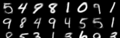
Figure 8: Generated Samples

As discussed in (Genevay et al.,, 2019), clusters may be used as an unsupervised classifier and accuracy is reported in Table 6, illustrating that the clusters are meaningful. In addition, samples from the clustered latent space may be used to generate new samples as a form of conditional generation, again shown in Figure 8.

Accuracy for each cluster is defined as in (Genevay et al.,, 2019), as follows. Accuracy for label $l$ in cluster $k$ is by $acc_{l,k}=\frac{\sum_{i}\mathbf{I}_{y_{i}==l,\tilde{y}_{i}==k}}{\sum_{i}\mathbf{I}_{y_{i}==k}}$ where $\tilde{y}_{i}=\arg\min_{k}||z_{i}-\mu_{\phi,k}||^{2}_{2}$ and $y_{i}$ is the true label of $x_{i}$. We write the top label accuracy for each cluster $k$ as $\max_{l}acc_{l,k}$. When using $10$ clusters for $10$ labels for MNIST, each cluster’s top label accuracy corresponds to a different label, one cluster for each digit. Table 6 shows that the clusters manage to capture geometrically meaningful information corresponding to each label.

Table 6: Evaluation Accuracy of trained clustered VAE for MNIST

Digit	0	1	2	3	4	5	6	7	8	9
Accuracy	0.91	0.66	0.42	0.56	0.80	0.61	0.68	0.64	0.90	0.78

Appendix C Overhead Analysis

Although timings are highly dependent on hardware and implementation, we provide some experimental examples running on a single V100 GPU and 4 CPUs. This shows that the time overhead for DualSort and Gaussian initializers are inconsequential relative to speed-up in terms of both time and iteration count for the savings in Sinkhorn iterations. The Gaussian mixture model (GMM) is computationally more expensive than the other proposed initializers, however the table below shows that it can also result in time savings.

C.1 Differentiable Sorting

Table 7: Average time in seconds for DualSort with 3 iterations and Sinkhorn iterations to convergence over 200 soft sorting problems of dimension $n$

$n$	Initializer	Initialization	Iterations
$32$	$\mathbf{0}$	-	$0.28$
	DualSort	$0.0012$	$0.22$
$64$	$\mathbf{0}$	-	$0.22$
	DualSort	$0.0012$	$0.088$
$128$	$\mathbf{0}$	-	$0.17$
	DualSort	$0.0012$	$0.066$
$256$	$\mathbf{0}$	-	$0.17$
	DualSort	$0.0012$	$0.049$
$512$	$\mathbf{0}$	-	$0.13$
	DualSort	$0.0012$	$0.050$
$1024$	$\mathbf{0}$	-	$0.14$
	DualSort	$0.0012$	$0.058$

It can be seen that the DualSort initialization procedure is extremely efficient and does not have significant impact on the total run-time. The timings above are averaged per OT problem over 200 runs with different seeds.

C.2 Gaussian and GMM

In this section we consider timings for the word embedding/ document similarity experiment.

For the GMM initializer, the pre-compute is the average time to compute each GMM (1 per document), divided by the number of OT problems. Each GMM is reused multiple times, so the cost is split. Each GMM was computed using scikit-learn (Pedregosa et al.,, 2011) on CPU, for lack of a convenient GPU implementation. There exists open-source GPU implementations of Gaussian mixture models for diagonal component covariance matrices which are significantly faster, and may be worth further investigation for more efficient implementation. Similarly, one may amortize inference in GMMs or provide a warm-start from a pooled GMM to initialize fitting the GMM. We use the default K-means initializer from scikit learn. The Initialization field reports the time to compute the approximate dual potentials given the GMM parameters.

For the Gaussian initializer, the mean and variance parameters are inexpensive to compute, hence were not computed and cached but instead computed repeatedly on the fly for each OT problem. Hence the total initialization compute time is reported in the Initialization column. Further computational savings could be made by caching the Gaussian parameters for each document. Note that the dimension for the Gaussian OT approximation is $d=50$ and given the Gaussian initialization is negligible here, it would also be negligible for lower dimensional settings.

Table 8: Time, in seconds, per OT problem split by task, averaged over $1,225$ OT problems, from each pair of $50$ documents from the Newsgroup 20 dataset with a subset of vocabulary of size $n$.

$n$	Initializer	Pre-compute	Initialization	Sinkhorn Iter.	Total
$2,000$	$\mathbf{0}$	-	-	$0.059$	$0.059$
	Subsample	-	$0.016$	$0.051$	$0.067$
	Gaus	-	$0.0028$	$0.045$	$0.048$
	GMM $K=10$	$0.0027$	$0.023$	$0.047$	$0.073$
	GMM $K=25$	$0.0037$	$0.026$	$0.035$	$0.065$
	GMM $K=50$	$0.0047$	$0.033$	$0.027$	$0.063$
$5,000$	$\mathbf{0}$	-	-	$0.28$	$0.28$
	Subsample	-	$0.048$	$0.15$	$0.20$
	Gaus	-	$0.0036$	$0.22$	$0.22$
	GMM $K=10$	$0.0035$	$0.013$	$0.23$	$0.24$
	GMM $K=25$	$0.0070$	$0.030$	$0.18$	$0.22$
	GMM $K=50$	$0.012$	$0.035$	$0.13$	$0.17$
$10,000$	$\mathbf{0}$	-	-	$1.05$	$1.05$
	Subsample	-	$0.082$	$0.45$	$0.53$
	Gaus	-	$0.0053$	$0.81$	$0.81$
	GMM $K=10$	$0.0042$	$0.013$	$0.86$	$0.88$
	GMM $K=25$	$0.012$	$0.019$	$0.70$	$0.73$
	GMM $K=50$	$0.022$	$0.035$	$0.56$	$0.62$

Appendix D Gaussian Potential

In this section we derive explicitly the Gaussian potential. The transport map $T$ solving the Monge problem (4) from a non-degenerate Gaussian measure $\mu=\mathcal{N}(\mathbf{m}_{\mu},\mathbf{\Sigma}_{\mu})$ to another Gaussian $\nu=\mathcal{N}(\mathbf{m}_{\nu},\mathbf{\Sigma}_{\nu})$ can be recovered in closed-form as $T^{\star}(x):=\mathbf{A}(x-\mathbf{m}_{\mu})+\mathbf{m}_{\nu}$, where $\mathbf{A}=\mathbf{\Sigma}^{-\frac{1}{2}}_{\mu}(\mathbf{\Sigma}^{\frac{1}{2}}_{\mu}\mathbf{\Sigma}_{\nu}\mathbf{\Sigma}^{\frac{1}{2}}_{\mu})^{\frac{1}{2}}\mathbf{\Sigma}^{-\frac{1}{2}}_{\mu}$, see e.g. (Peyré et al.,, 2019, Chapter 2.6) for a discussion. Brenier’s theorem (Brenier,, 1987) states that for cost $c:(x,y)\rightarrow\frac{\|x-y\|^{2}}{2}$ this map is uniquely defined as the gradient of a convex function $\varphi$, and it can be verified that $T^{\star}(x)=\nabla\varphi(x)$ where $\varphi(x)=\frac{1}{2}(x-m_{\mu})^{T}\mathbf{A}(x-m_{\mu})+m_{\nu}^{T}x$.

The convex function $\varphi(x)$ is related to dual potential $f$ through $\varphi(x)=\frac{||x||^{2}}{2}-f(x)$ hence

$$f^{\star}(x)=\frac{||x||^{2}}{2}-\frac{1}{2}(x-m_{\mu})^{T}\mathbf{A}(x-m_{\mu})-m_{\nu}^{T}x.$$

For cost $c:(x,y)\rightarrow\|x-y\|^{2}$, the optimal potential is therefore

$$f^{\star}(x)=||x||^{2}-(x-m_{\mu})^{T}\mathbf{A}(x-m_{\mu})-2m_{\nu}^{T}x.$$

Appendix E Convergence of Sorting Initializer and DualSort Details

E.1 Proof of Primal Dual Convergence

Recovering optimal dual potentials corresponding to the primal solution is equivalent to finding any vector of shortest paths $\mathbf{f}$ from a single node e.g. node 1, in the network to each of the other nodes, see e.g. (Bertsimas and Tsitsiklis,, 1997, Theorem 7.17) and (Ahuja et al.,, 1988, Chapter 9).

Algorithm 3 computes the shortest path using a particular case of a method known as label correcting (Bertsimas and Tsitsiklis,, 1997, Chapter 7). Given there are no cycles, the proposed method recovers the shortest path by (Bertsimas and Tsitsiklis,, 1997, Theorem 7.18) and hence recovers the optimal dual potentials.

Algorithm 3 exploits the primal solution efficiently by correcting all nodes in the same tree, hence the iterations are dependent on the number of trees and not necessarily the number of nodes.

The minimization step, $\mathbf{f}_{s(k)}\leftarrow\min_{j}c_{s(k),j}-c_{\iota(j),j}+\mathbf{f}_{\iota(j)}$ follows traditional label correcting methods. However, a key insight is updating nodes along tree of $s(k)$ is equivalent to updating the minimum path to each node in the tree.

$\mathbf{f}_{i}$ is the shortest path to node $i$ if $\mathbf{f}_{i}\leq c_{i,j}-c_{\iota(j),j}+\mathbf{f}_{\iota(j)}$ $\forall j$, which is equivalent to $\mathbf{f}_{i}+\mathbf{g}_{j}\leq c_{i,j}$ and may be interpreted as $\mathbf{f}_{i}$ being less than the route to any other source node $\mathbf{f}_{\iota(j)}$ then to $\mathbf{f}_{i}$ via sink node $j$, at cost $c_{i,j}-c_{\iota(j),j}$.

E.2 DualSort Algorithm

The DualSort algorithm is given sequentially below in Algorithm 2. Without loss of generality, we assume that $x_{i}$ is rearranged in increasing order, so that the sorting permutation $\sigma$ is the identity. Let diag denote the operator used to extract the diagonal of a matrix, so that $\textrm{diag}(\mathbf{C})\in\mathbb{R}^{n}$ and one has $[\textrm{diag}(\mathbf{C})]_{i}=c_{i,i}$, and write $\mathbf{1}$ for the vector of size $n$ with all entries $1$. The inner loop can be carried out in two different ways, either using a vectorized update or looping through coordinates one at a time. These two updates are distinct, and we do observe that cycling through coordinates in Gauss-Seidel fashion converges faster in terms of total number of updates. However, that perspective misses the fact that vectorized updates utilize more efficiently accelerators from a runtime perspective. Additionally, these updates are equal to, in terms of complexity to the Sinkhorn iterations, making it easier to discuss the benefits of our initializers. For these reasons, we use the vectorized=True flag in our experiments.

1:  Input: Cost matrix $\mathbf{C}$, primal solution, $\mathbf{P}$, vectorized flag

2:  Initialize: $\mathbf{f}=0$

3:  while not converged do

4:     if vectorized then

5:        $\mathbf{f}\leftarrow\min_{\text{axis=1}}\left(\mathbf{C}-\textrm{diag}(\mathbf{C})\mathbf{1}^{T}+\mathbf{f}\mathbf{1}^{T}\right)$

6:     else

7:        for $i\in\{1,\ldots,n\}$ do

8:           $\mathbf{f}_{i}\leftarrow\left(\min_{j}c_{i,j}-c_{j,j}+\mathbf{f}_{j}\right)$

9:        end for

10:     end if

11:  end while

12:  Return $\mathbf{f}$

Algorithm 5 DualSort Initializer

E.3 Number of DualSort Iterations

Figure 9 illustrates the convergence of the DualSort algorithm when compared to the true potentials found from linear programming. Visually, from the right plot of Figure 9, the approximate dual is close to the true dual after just one iteration. However the squared error (left plot) is still large. After $3$ iterations, the error is significantly reduced and after $10$, the error is not noticeable.

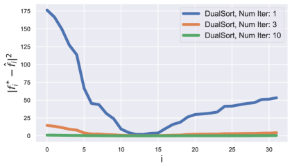
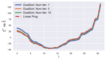
Figure 9: Single sample of size 32 from Gaussian blob dataset with 5 centers. Left: squared error vs true potential by number of DualSort iterations. Right: Potential from linear solver vs DualSort approximations.

Figure 10 shows how the performance of the initializer improves significantly from $1$ initialization iteration to $3$ or $10$ for the CIFAR-100 soft-error classification task. Here performance is measured in how many additional Sinkhorn iterations are required after initialization for convergence. Note however that empirically there is not much difference between $3$ and $10$, hence $3$ was used in experiments.

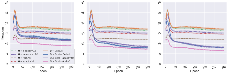
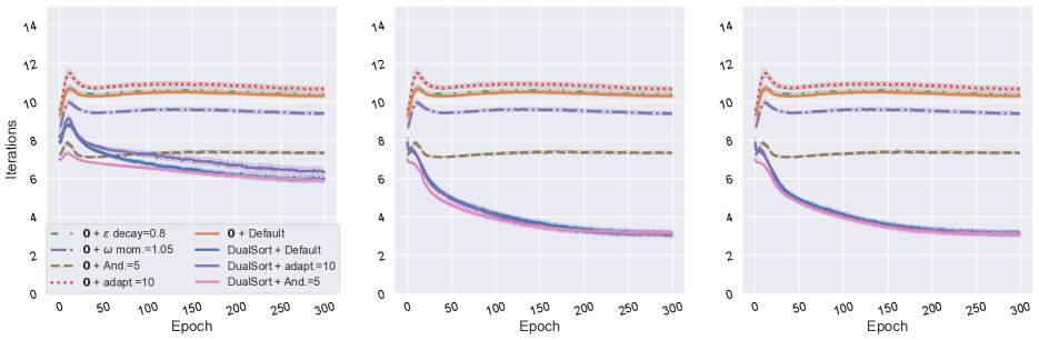
Figure 10: Number of Sinkhorn iterations per training step when using soft error loss for CIFAR-100 classifier. Top: threshold=0.01, bottom: threshold=0.05. Number of vectorized DualSort iterations 1,3,10 (left to right)

Appendix F Threshold Analysis

Convergence of each the Sinkhorn for each problem was determined according to a threshold tolerance, $\tau$, for how close the marginals from the coupling derived from potentials are to the true marginals. For OT problem between $\mu=\sum_{i=1}^{n}a_{i}\delta_{x_{i}}$ and $\nu=\sum_{j=1}^{n}b_{i}\delta_{y_{j}}$, and denote potentials after $l$ Sinkhorn iterations as $\mathbf{f}^{(l)}$, $\mathbf{g}^{(l)}$, then the corresponding coupling may be written elementwise as $\mathbf{p}^{(l)}_{i,j}=\exp{\frac{\mathbf{f}^{(l)}_{i}+\mathbf{g}^{(l)}_{j}-c_{i,j}}{\epsilon}}$ and the threshold condition may be written

$$\sum_{i}\lvert\sum_{j}\mathbf{p}^{(l)}_{i,j}-a_{i}\rvert+\sum_{j}\lvert\sum_{i}\mathbf{p}^{(l)}_{i,j}-b_{j}\rvert<\tau.$$

We use $\tau=0.01$ for speed. But also note that a higher threshold $\tau=0.05$ leads to faster convergence without drop in performance, as evidenced in Figure 11 for the soft error classification task on CIFAR-100. Figure 10 also illustrates that the DualSort initializer appears to exhibit relatively better performance to the zero initialization for a higher convergence threshold.

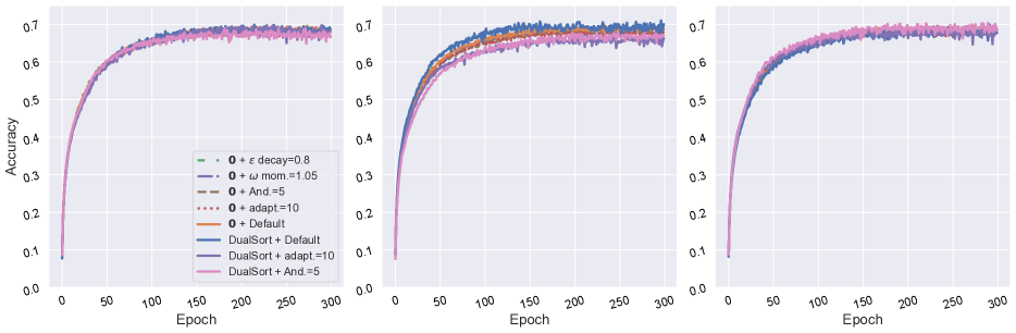
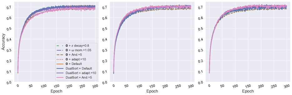
Figure 11: Evaluation accuracy through training when using soft error loss for CIFAR-100 classifier. Top: threshold=0.01, bottom: threshold=0.05. Number of vectorized DualSort iterations 1,3,10 (left to right)

Appendix G Other Details

Societal Impact. We are not aware of any direct negative societal impacts in this work. We acknowledge that the Sinkhorn algorithm may be used in various applications across compute vision and tracking with negative impacts, and this work may enable further such applications.
Code. Code for initializers has been incorporated into OTT library (Cuturi et al.,, 2022).
Open source software and licences. (Cuturi et al.,, 2022) has an Apache licence.

References

- Adams and Zemel, (2011) Adams, R. P. and Zemel, R. S. (2011). Ranking via sinkhorn propagation. arXiv preprint arXiv:1106.1925.
- Ahuja et al., (1988) Ahuja, R. K., Magnanti, T. L., and Orlin, J. B. (1988). Network flows.
- Altschuler et al., (2019) Altschuler, J., Bach, F., Rudi, A., and Niles-Weed, J. (2019). Massively scalable sinkhorn distances via the nyström method. Advances in neural information processing systems, 32.
- Amos et al., (2022) Amos, B., Cohen, S., Luise, G., and Redko, I. (2022). Meta optimal transport.
- Anderson, (1965) Anderson, D. G. (1965). Iterative procedures for nonlinear integral equations. Journal of the ACM (JACM), 12(4):547–560.
- Bertsimas and Tsitsiklis, (1997) Bertsimas, D. and Tsitsiklis, J. N. (1997). Introduction to linear optimization, volume 6. Athena Scientific Belmont, MA.
- Bradbury et al., (2018) Bradbury, J., Frostig, R., Hawkins, P., Johnson, M. J., Leary, C., Maclaurin, D., Necula, G., Paszke, A., VanderPlas, J., Wanderman-Milne, S., et al. (2018). Jax: composable transformations of python+ numpy programs. Version 0.2, 5:14–24.
- Brenier, (1987) Brenier, Y. (1987). Décomposition polaire et réarrangement monotone des champs de vecteurs. CR Acad. Sci. Paris Sér. I Math., 305:805–808.
- Caron et al., (2020) Caron, M., Misra, I., Mairal, J., Goyal, P., Bojanowski, P., and Joulin, A. (2020). Unsupervised learning of visual features by contrasting cluster assignments. Advances in Neural Information Processing Systems, 33:9912–9924.
- Chen et al., (2018) Chen, Y., Georgiou, T. T., and Tannenbaum, A. (2018). Optimal transport for gaussian mixture models. IEEE Access, 7:6269–6278.
- Chiappori et al., (2017) Chiappori, P.-A., McCann, R. J., and Pass, B. (2017). Multi-to one-dimensional optimal transport. Communications on Pure and Applied Mathematics, 70(12):2405–2444.
- Chizat et al., (2020) Chizat, L., Roussillon, P., Léger, F., Vialard, F.-X., and Peyré, G. (2020). Faster wasserstein distance estimation with the sinkhorn divergence. Advances in Neural Information Processing Systems, 33:2257–2269.
- Corenflos et al., (2021) Corenflos, A., Thornton, J., Deligiannidis, G., and Doucet, A. (2021). Differentiable particle filtering via entropy-regularized optimal transport. In International Conference on Machine Learning, pages 2100–2111. PMLR.
- Courty et al., (2017) Courty, N., Flamary, R., Habrard, A., and Rakotomamonjy, A. (2017). Joint distribution optimal transportation for domain adaptation. Advances in Neural Information Processing Systems, 30.
- Courty et al., (2014) Courty, N., Flamary, R., and Tuia, D. (2014). Domain adaptation with regularized optimal transport. In Joint European Conference on Machine Learning and Knowledge Discovery in Databases, pages 274–289. Springer.
- Cuturi, (2013) Cuturi, M. (2013). Sinkhorn distances: Lightspeed computation of optimal transport. Advances in neural information processing systems, 26.
- Cuturi et al., (2022) Cuturi, M., Meng-Papaxanthos, L., Tian, Y., Bunne, C., Davis, G., and Teboul, O. (2022). Optimal transport tools (ott): A jax toolbox for all things wasserstein. arXiv preprint arXiv:2201.12324.
- Cuturi and Peyré, (2015) Cuturi, M. and Peyré, G. (2015). A smoothed dual approach for variational wasserstein problems. arXiv preprint arXiv:1503.02533.
- Cuturi et al., (2020) Cuturi, M., Teboul, O., Niles-Weed, J., and Vert, J.-P. (2020). Supervised quantile normalization for low rank matrix factorization. In International Conference on Machine Learning, pages 2269–2279. PMLR.
- Cuturi et al., (2019) Cuturi, M., Teboul, O., and Vert, J.-P. (2019). Differentiable ranking and sorting using optimal transport. Advances in neural information processing systems, 32.
- Dantzig et al., (1956) Dantzig, G. B., Ford Jr, L. R., and Fulkerson, D. R. (1956). A primal–dual algorithm. Technical report, RAND CORP SANTA MONICA CA.
- Deng, (2012) Deng, L. (2012). The mnist database of handwritten digit images for machine learning research. IEEE Signal Processing Magazine, 29(6):141–142.
- d’Aspremont et al., (2021) d’Aspremont, A., Scieur, D., Taylor, A., et al. (2021). Acceleration methods. Foundations and Trends® in Optimization, 5(1-2):1–245.
- Feydy, (2020) Feydy, J. (2020). Geometric data analysis, beyond convolutions. PhD thesis, Université Paris-Saclay Gif-sur-Yvette, France.
- Flamary et al., (2021) Flamary, R., Courty, N., Gramfort, A., Alaya, M. Z., Boisbunon, A., Chambon, S., Chapel, L., Corenflos, A., Fatras, K., Fournier, N., et al. (2021). Pot: Python optimal transport. Journal of Machine Learning Research, 22(78):1–8.
- Genevay et al., (2019) Genevay, A., Dulac-Arnold, G., and Vert, J.-P. (2019). Differentiable deep clustering with cluster size constraints. arXiv preprint arXiv:1910.09036.
- Genevay et al., (2018) Genevay, A., Peyré, G., and Cuturi, M. (2018). Learning generative models with sinkhorn divergences. In International Conference on Artificial Intelligence and Statistics, pages 1608–1617. PMLR.
- Hashimoto et al., (2016) Hashimoto, T., Gifford, D., and Jaakkola, T. (2016). Learning Population-Level Diffusions with Generative Recurrent Networks. volume 33.
- Higham, (2008) Higham, N. J. (2008). Functions of matrices: theory and computation. SIAM.
- Janati et al., (2020) Janati, H., Bazeille, T., Thirion, B., Cuturi, M., and Gramfort, A. (2020). Multi-subject meg/eeg source imaging with sparse multi-task regression. NeuroImage, 220:116847.
- Kingma et al., (2014) Kingma, D. P., Mohamed, S., Jimenez Rezende, D., and Welling, M. (2014). Semi-supervised learning with deep generative models. Advances in neural information processing systems, 27.
- Kosowsky and Yuille, (1994) Kosowsky, J. and Yuille, A. L. (1994). The invisible hand algorithm: Solving the assignment problem with statistical physics. Neural networks, 7(3):477–490.
- Kusner et al., (2015) Kusner, M., Sun, Y., Kolkin, N., and Weinberger, K. (2015). From word embeddings to document distances. In International conference on machine learning, pages 957–966. PMLR.
- Lang, (1995) Lang, K. (1995). Newsweeder: Learning to filter netnews. In Proceedings of the Twelfth International Conference on Machine Learning, pages 331–339.
- Lehmann et al., (2021) Lehmann, T., Von Renesse, M.-K., Sambale, A., and Uschmajew, A. (2021). A note on overrelaxation in the sinkhorn algorithm. Optimization Letters, pages 1–12.
- Luise et al., (2018) Luise, G., Rudi, A., Pontil, M., and Ciliberto, C. (2018). Differential properties of sinkhorn approximation for learning with wasserstein distance. Advances in Neural Information Processing Systems, 31.
- Meyron, (2019) Meyron, J. (2019). Initialization procedures for discrete and semi-discrete optimal transport. Computer-Aided Design, 115:13–22.
- Monge, (1781) Monge, G. (1781). Mémoire sur la théorie des déblais et des remblais. Histoire de l’Académie Royale des Sciences, pages 666–704.
- Pedregosa et al., (2011) Pedregosa, F., Varoquaux, G., Gramfort, A., Michel, V., Thirion, B., Grisel, O., Blondel, M., Prettenhofer, P., Weiss, R., Dubourg, V., Vanderplas, J., Passos, A., Cournapeau, D., Brucher, M., Perrot, M., and Duchesnay, E. (2011). Scikit-learn: Machine learning in Python. Journal of Machine Learning Research, 12:2825–2830.
- Pennington et al., (2014) Pennington, J., Socher, R., and Manning, C. D. (2014). Glove: Global vectors for word representation. In Empirical Methods in Natural Language Processing (EMNLP), pages 1532–1543.
- Peyré et al., (2019) Peyré, G., Cuturi, M., et al. (2019). Computational optimal transport: With applications to data science. Foundations and Trends® in Machine Learning, 11(5-6):355–607.
- Pooladian and Niles-Weed, (2021) Pooladian, A.-A. and Niles-Weed, J. (2021). Entropic estimation of optimal transport maps.
- Salimans et al., (2018) Salimans, T., Zhang, H., Radford, A., and Metaxas, D. (2018). Improving GANs using optimal transport. In International Conference on Learning Representations.
- Sander et al., (2022) Sander, M. E., Ablin, P., Blondel, M., and Peyré, G. (2022). Sinkformers: Transformers with doubly stochastic attention. In International Conference on Artificial Intelligence and Statistics, pages 3515–3530. PMLR.
- Santambrogio, (2015) Santambrogio, F. (2015). Optimal transport for applied mathematicians. Birkhauser.
- Sarlin et al., (2020) Sarlin, P.-E., DeTone, D., Malisiewicz, T., and Rabinovich, A. (2020). Superglue: Learning feature matching with graph neural networks. In Proceedings of the IEEE/CVF Conference on Computer Vision and Pattern Recognition (CVPR).
- Scetbon and Cuturi, (2020) Scetbon, M. and Cuturi, M. (2020). Linear time sinkhorn divergences using positive features. Advances in Neural Information Processing Systems, 33:13468–13480.
- Schiebinger et al., (2019) Schiebinger, G., Shu, J., Tabaka, M., Cleary, B., Subramanian, V., Solomon, A., Gould, J., Liu, S., Lin, S., Berube, P., et al. (2019). Optimal-Transport Analysis of Single-Cell Gene Expression Identifies Developmental Trajectories in Reprogramming. Cell, 176(4).
- Schmitz et al., (2018) Schmitz, M. A., Heitz, M., Bonneel, N., Ngole, F., Coeurjolly, D., Cuturi, M., Peyré, G., and Starck, J.-L. (2018). Wasserstein dictionary learning: Optimal transport-based unsupervised nonlinear dictionary learning. SIAM Journal on Imaging Sciences, 11(1):643–678.
- Schmitzer, (2019) Schmitzer, B. (2019). Stabilized sparse scaling algorithms for entropy regularized transport problems. SIAM Journal on Scientific Computing, 41(3):A1443–A1481.
- Sejourne et al., (2022) Sejourne, T., Vialard, F.-X., and Peyré, G. (2022). Faster unbalanced optimal transport: Translation invariant sinkhorn and 1-d frank-wolfe. In Camps-Valls, G., Ruiz, F. J. R., and Valera, I., editors, Proceedings of The 25th International Conference on Artificial Intelligence and Statistics, volume 151 of Proceedings of Machine Learning Research, pages 4995–5021. PMLR.
- Sinkhorn, (1967) Sinkhorn, R. (1967). Diagonal equivalence to matrices with prescribed row and column sums. American Mathematical Monthly, 74:402–405.
- Solomon et al., (2015) Solomon, J., De Goes, F., Peyré, G., Cuturi, M., Butscher, A., Nguyen, A., Du, T., and Guibas, L. (2015). Convolutional Wasserstein distances: efficient optimal transportation on geometric domains. ACM Transactions on Graphics, 34(4):66:1–66:11.
- Thibault et al., (2021) Thibault, A., Chizat, L., Dossal, C., and Papadakis, N. (2021). Overrelaxed sinkhorn–knopp algorithm for regularized optimal transport. Algorithms, 14(5):143.
- (55) Xie, Y., Dai, H., Chen, M., Dai, B., Zhao, T., Zha, H., Wei, W., and Pfister, T. (2020a). Differentiable top-k with optimal transport. In Larochelle, H., Ranzato, M., Hadsell, R., Balcan, M., and Lin, H., editors, Advances in Neural Information Processing Systems, volume 33, pages 20520–20531. Curran Associates, Inc.
- (56) Xie, Y., Wang, X., Wang, R., and Zha, H. (2020b). A fast proximal point method for computing exact wasserstein distance. In Uncertainty in artificial intelligence, pages 433–453. PMLR.