The geometry of planar linear flows

Abstract

We identify incompressible planar linear flows that are generalizations of the well known one-parameter family characterized by the ratio of in-plane extension to (out-of-plane) vorticity. The latter ‘canonical’ family is classified into elliptic and hyperbolic linear flows with closed and open streamlines, respectively, corresponding to the extension-to-vorticity ratio being less or greater than unity; unity being the marginal case of simple shear flow. The novel flows possess an out-of-plane extension, but the streamlines may nevertheless be closed or open, allowing for an organization, in a three-dimensional parameter space, into regions of ‘eccentric’ elliptic and hyperbolic flows, separated by a surface of degenerate linear flows with parabolic streamlines that are generalizations of simple shear. We discuss implications for various fluid mechanical scenarios.

The one-parameter planar linear flow family is an important class of incompressible flows illustrating the fluid mechanical consequences of varying the relative magnitudes of extension and vorticityLealBook ; Kao ; Bentley ; Marath2 . Limiting members include planar extension (zero vorticity) and solid body rotation (zero extension) with simple shear, the transitional member with straight streamlines, separating hyperbolic and elliptic flows with open and closed streamlines, respectively. The planar linear flow family is of particular importance in microhydrodynamics; the microstructural element of a sheared complex fluid sees a local linear flow, and for an ambient two-dimensional flow, this must be one of the planar linear flows. Simple shear is rheologically significant, being the flow topology generated in standard rheometric devices. Drop deformation and break-up in planar linear flows have been extensively studiedTaylor ; Bentley2 ; Bentley ; RallisonRev ; StoneRev ; recent efforts focus on vesiclesdechampssteinberg2009 ; ZabuskySteinberg2011 ; vivek2019 and the hysteretic dynamics of macromolecules in these flowsLarson ; Shaqfeh1 ; Chu ; Shaqfeh2 ; HurShaqfeh2002 ; ChuShaqfeh2003 ; HoffmanShaqfeh2007 . Planar linear flows highlight diffusion-limited transport from suspended particles and drops in the Stokesian regimeFrankel1 ; Acrivos ; Poe ; Deepak1 , thereby emphasizing the role of streamline topology in convective enhancementSub1 ; Sub2 ; Deepak1 ; Deepak2 ; Mahan . These flows are crucial to dilute suspension rheology -​ closed pathlines in the two-sphere problemBatchelor ; Kao and closed (Jeffery) orbits of an axisymmetric particleJeffery ; Bretherton ; Hinch1 ; Hinch2 , in subsets of these flows, lead to an indeterminate stress in the pure-hydrodynamic limitBatchelor2 ; Brady ; Bergenholtz , rendering the rheology sensitive to departures from Stokesian hydrodynamicsBatchelor2 ; Bergenholtz ; SubBrady2006 ; Hinch1 ; Marath1 ; Marath2 ; Marath3 . The above examples showcase the importance of what, from hereon, is termed the canonical planar linear flow family. It forms an integral element of any flow-classification scheme based on microstructural evolutionOlbricht .

A linear flow is defined by $\!\bm{u}\!=\!\bm{\Gamma}\!\bm{\cdot}\!\bm{x}$, $\bm{\Gamma}$ being the transpose of the velocity gradient tensor. $\bm{\Gamma}\!\!=\!\!\left[\!\begin{smallmatrix}0&1&0&\\ \hat{\alpha}&0&0\\ 0&0&0\!\end{smallmatrix}\!\right]$ for canonical planar linear flows with $\hat{\alpha}\!\!\in\!\![-1,1]$;​ $\frac{(1+\hat{\alpha})}{(1-\hat{\alpha})}$ denotes the ratio of in-plane extension to (out-of-plane) vorticity. The eigenvalues of $\bm{\Gamma}$, $\mu_{i}\!\!\equiv\!\!\!\{-\sqrt{\hat{\alpha}},\sqrt{\hat{\alpha}},0\}$, imply a trivial cubic invariant ($R\!=\!\mu_{1}\mu_{2}\mu_{3}\!=\!0$), with the quadratic invariant $Q\!\!=\!\!\mu_{1}\mu_{2}\!+\!\mu_{2}\mu_{3}\!+\!\mu_{1}\mu_{3}\!\!=\!\!-\hat{\alpha}$ determining the nature of the flow. In the $QR$-classification of incompressible linear flowsPerry ; Cantwell , canonical planar linear flows lie on the $Q$-axis:$Q\!\!>\!\!0$ and $Q\!<\!0$ correspond to canonical elliptic and hyperbolic linear flows, respectively, with the streamlines being planar ellipses and hyperbolae; $Q\!=\!0$ corresponds to simple shear. Incompressible linear flows are uniquely characterized by their surface streamline topologies, obtained by projecting the 3D streamline pattern onto a unit sphere. As shown in Fig. 1b, surface streamlines for canonical elliptic flows are spherical ellipses or Jeffery orbitsJeffery ; Bretherton , with the geometrical aspect ratio replaced by an effective one ($\!1/\!\sqrt{-\hat{\alpha}}$) in terms of the flow-type parameter. Those for hyperbolic flows are open, and may be regarded as orbits with imaginary aspect ratiosDeepak1 ; simple shear yields a meridional surface-streamline topology. The origin, a fixed point in the dynamical systems parlancePerry , is a center for canonical elliptic flows and a saddle for hyperbolic ones, with eigenvectors:$\bm{v_{1}}\!=\!\{-(\sqrt{\hat{\alpha}})^{-1},1,0\}$; ​​$\bm{v_{2}}\!=\!\{(\sqrt{\hat{\alpha}})^{-1},1,0\}$; ​​$\bm{v_{3}}\!=\!\{0,0,1\}$. The vorticity $\bm{\omega}$ is normal to the flow plane, and aligned with the neutral eigenvector ($\bm{v_{3}}$); see suppmaterial .

Figure 1: Surface (red) and 3D (blue) streamlines of (a) eccentric ($\alpha\!=\!4\sqrt{2},\epsilon\!=\!-2,\theta_{\omega}\!=\!\pi/3,\phi_{\omega}\!=\!0$) and (b) canonical ($\hat{\alpha}=-0.5$) elliptic linear flows. (c) The neutral and inclined elliptical cones for the eccentric case; ${\boldsymbol{v}}_{3}$ lies on the neutral (circular)cone, and is the axis of the inclined elliptical cone of streamlines; $E_{i}(i\!=\!1\!-\!3)$ are the principal extensions.

We report generalizations of the canonical planar linear flows above, where streamlines are plane (quadratic) curves despite a non-trivial extensional component normal to the flow plane. The existence of these novel flows is most easily understood for the elliptic case, the surface streamline topology for which is shown in Fig. 1a; despite again being spherical ellipses, the eccentric disposition of the surface streamlines is in contrast to the concentric arrangement in the canonical case(Fig. 1b). The limiting surface streamlines in both cases comprise a great circle and the point in which $\bm{v_{3}}$ intersects the unit sphere. But, $\bm{v_{3}}$ for the eccentric case is neither aligned with ${\bm{\omega}}$, nor orthogonal to the plane of the flow.

The ‘eccentric’ elliptic linear flow (Fig. 1a) may be rationalized by first noting that a $3D$ extensional flow has an associated cone of neutral directions (${\boldsymbol{n}}$), defined by ${\boldsymbol{\Gamma}}\!\!:\!\!{\boldsymbol{n}}{\boldsymbol{n}}\!=\!0$. The cone, a circular one for axisymmetric extension and an elliptical one in general, separates regions with positive and negative rates of stretch; its interior corresponds to a positive rate of stretch when the largest (in magnitude) eigenvalue is positive. For $\boldsymbol{\omega}\!=\!0$, any material point comes from, and goes to, infinity, crossing the neutral cone in the process. But, for an appropriately oriented ${\boldsymbol{\omega}}$ of the right magnitude, a material point traverses a closed curve, since the line element connecting this point to the origin samples regions within and outside the cone such that the net rate of stretch over a $2\pi$-circuit is zero. Linearity of the flow implies that this curve is an ellipse, and that all streamlines are geometrically similar ellipses (the blue curves in Fig.1a); ${\boldsymbol{v}}_{3}$ lies on the neutral cone, the line along ${\boldsymbol{v}}_{3}$ being the locus of ellipse centers(Fig.1c). Each surface streamline is the projection of closed streamlines on an inclined elliptical cone with axis along ${\boldsymbol{v}}_{3}$. Elliptical double cones, with the vertex solid angle ranging from zero (the straight line along ${\boldsymbol{v}}_{3}$) to $2\pi$ (the plane of the flow), foliate 3D space.

In the canonical case, the aforementioned neutral cone opens out into a pair of planes($x_{1}\!=\!\!0;x_{2}\!=\!\!0$) orthogonal to the flow plane. For sufficiently large $|{\boldsymbol{\omega}}|$, any line element precesses about the $x_{3}$-axis, spending equal times in quadrants of positive ($x_{1}x_{2}>0$) and negative ($x_{1}x_{2}<0$) rates of stretch, automatically satisfying the net zero rate of stretch required for a closed elliptical streamline. Reducing $|{\boldsymbol{\omega}}|$ leads to increasingly elongated ellipses that degenerate to straight lines (simple shear) at a threshold $|{\boldsymbol{\omega}}|$ (for $\hat{\alpha}=0)$; canonical hyperbolic flows arise for smaller $|{\boldsymbol{\omega}}|$. An analogous argument implies the existence of eccentric hyperbolic flows(Fig.2a), although one needs to reorient ${\boldsymbol{\omega}}$, while decreasing its magnitude, so the flow remains planar. Simple shear is replaced by a degenerate linear flow with parabolic streamlines  at the threshold(Fig.2b).

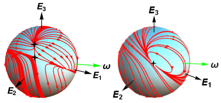
Figure 2: Surface streamlines of (a) eccentric hyperbolic ($\alpha\!\approx\!2.963,\epsilon\!=\!-2,\theta_{\omega}\!=4\pi/9,\phi_{\omega}\!=\!0$) and (b) parabolic ($\alpha\!=\!2\sqrt{3},\epsilon\!=\!-2,\theta_{\omega}\!=\!\tan^{-1}2\sqrt{2},\phi_{\omega}\!=\!0$) planar linear flows.

Eccentric planar linear flows have $R=0$, with $Q\!>\!0\,(<\!0)$ for eccentric elliptic (hyperbolic) flows. So, the $QR$-classification Perry ; Cantwell has canonical and eccentric planar linear flows in identical intervals on the $Q$-axis, highlighting the drawback of a scalar-invariant-based classification - the lack of ‘structural’ information, and the notion of a distance between flows. While this issue may be resolved for canonical compressible planar linear flowsFairlie ; Strogatz without enlarging the original parameter space (see suppmaterial ), three-dimensional flows require an alternate larger set of structural parametersTsinober2009 ; Meneveau . A convenient choice for incompressible linear flows is:​​ $\epsilon\!\!=\!\!E_{3}/E_{2}$ measuring the non-axisymmetry of the rate of strain tensor ${\bm{E}}$;$\alpha\!=\!|\bm{\omega}|/E_{2}$ measuring the vorticity magnitude (the analog of $2\frac{(1-\hat{\alpha})}{(1+\hat{\alpha})}$ for the canonical case);and angles ($\theta_{\omega},\phi_{\omega}$) characterizing the orientation of $\bm{\omega}$ in rate-of-strain-aligned coordinates; see Fig.3(center). Incompressible linear flows exist in an $(\epsilon,\alpha,\theta_{\omega},\phi_{\omega})$-hyperspace with :

$$\bm{\Gamma}=\begin{bmatrix}-(1+\epsilon)&-\frac{\alpha\cos\theta_{\omega}}{2}&-\frac{\alpha\sin\theta_{\omega}\sin\phi_{\omega}}{2}\\ \frac{\alpha\cos\theta_{\omega}}{2}&1&-\frac{\alpha\sin\theta_{\omega}\cos\phi_{\omega}}{2}\\ \frac{\alpha\sin\theta_{\omega}\sin\phi_{\omega}}{2}&\frac{\alpha\sin\theta_{\omega}\cos\phi_{\omega}}{2}&\epsilon\end{bmatrix}.$$ (1)

Accounting for axes relabeling, and invariance to an overall sign change, all flow topologies are covered for $\epsilon\!\in\![-2,0]$, $\alpha\!\geq\!0$, $\theta_{\omega},\phi_{\omega}\!\in\![0,\!\pi/2]$; $(\epsilon,\alpha,\theta_{\omega},\phi_{\omega})\!\equiv\!(0,\alpha,0,\phi_{\omega})$ and $(-1,\alpha,\frac{\pi}{2},0)$ correspond to canonical planar linear flows, with $\alpha=2$ for simple shear; $\alpha=0$ yields linear extensional flows parameterized by $\epsilon$Deepak1 , $\epsilon\!=\!-2$ being axisymmetric extension.

We characterize planar linear flows in the above hyperspace, beginning with expressions for the invariants:

$$Q\!=\!\frac{\alpha^{2}}{4}-(1+\epsilon+\epsilon^{2}),$$ (2)

$$R\!=\!\frac{\epsilon(\!8(1\!+\!\epsilon)\!\!-\!\frac{\alpha^{2}}{2}(1\!+\!\!3\cos\theta_{\omega})\!)\!+\!\!(2\!+\!\epsilon)\alpha^{2}\!\cos 2\phi_{\omega}\!\sin^{2}\!\theta_{\omega}}{8}\!.$$ (3)

Planar linear flows exist in the subspace $R=0$ corresponding to:

$$\alpha\! =\!\!\frac{4\sqrt{\epsilon(1+\epsilon)}}{[\cos 2\theta_{\omega}(3\epsilon\!+\!(2\!+\!\epsilon\!)\!\cos\!2\phi_{\omega})\!\!+\!\!(\epsilon\!-\!(2\!+\!\epsilon\!)\!\cos\!2\phi_{\omega})]^{\frac{1}{2}}}.$$ (4)

The inability to visualize the volume defined by (4), in a 4D-hyperspace, leads us to depict the domain of planar linear flows via its projections onto $\epsilon\!-\!\phi_{\omega}\!-\!\theta_{\omega}$ and $\epsilon\!-\!\phi_{\omega}\!-\!1/\alpha$ subspaces(Figs.3a and b).

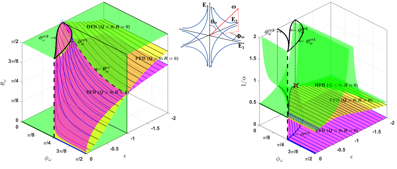
Figure 3: The planar linear flow domain in the (a) $\epsilon-\phi_{\omega}-\theta_{\omega}$ and (b) $\epsilon-\phi_{\omega}-1/\alpha$ sub-spaces. HFB PFB and EFB denote Hyperbolic, Parabolic and Elliptic Flow Boundaries. The central sketch depicts the flow-type parameters that characterize incompressible linear flows.

Assuming one boundary of $R=0$ to correspond to solid-body rotation, and using $1/\alpha=0$ in (4), leads to

$$\theta^{cr1}_{\omega} =\frac{1}{2}\cos^{-1}\left(\frac{(2+\epsilon)\cos 2\phi_{\omega}-\epsilon}{3\epsilon+(2+\epsilon)\cos 2\phi_{\omega}}\right),$$ (5)

which is real-valued for $\phi_{\omega}\geq\phi_{\omega}^{cr1}\!(\epsilon)\!=\!\frac{1}{2}\!\cos^{-1}\!\!\left(\!\frac{-\epsilon}{2+\epsilon}\!\right)$ for $\epsilon\!\!\in\!\![-1,0]$; $\theta^{cr1}_{\omega}\!=\!\frac{\pi}{2}$ for $\phi_{\omega}\!=\!\phi_{\omega}^{cr1}\!(\epsilon)$. The curves [$\theta_{\omega}\!=\!\frac{\pi}{2},\phi_{\omega}^{cr1}\!(\epsilon)]$ and $[1/\alpha\!=\!0,\phi_{\omega}^{cr1}\!(\epsilon)]$, for $\epsilon\!\in\![-1,0]$, therefore mark the edge of the parts of the boundary, comprising solid-body rotation, in the $\epsilon\!-\!\phi_{\omega}\!-\!\theta_{\omega}$ and $\epsilon\!-\!\phi_{\omega}\!-\!1/\alpha$ subspaces. The boundary for $\phi_{\omega}<\phi_{\omega}^{cr1}\!(\epsilon)$ consists of finite-$\alpha$ eccentric elliptic flows. It is the plane $\theta_{\omega}\!=\!\frac{\pi}{2}$ in the former subspace, and given by:

$$\frac{1}{\alpha^{cr1}}=\frac{\sqrt{\epsilon+(2+\epsilon)\cos 2\phi_{\omega}}}{2\sqrt{-2\epsilon(1+\epsilon)}},$$ (6)

in the latter one (obtained by setting $\theta_{\omega}\!=\!\frac{\pi}{2}$ in (4)). In both subspaces, the boundary ends in an intersection with the parabolic-flow surface obtained next. The curves of intersection are $[\theta_{\omega}\!=\!\frac{\pi}{2},\phi_{\omega}^{cr2}\!(\epsilon)]$ and $[1/\alpha\!=\!1/(2\!\sqrt{1\!+\!\epsilon\!+\!\epsilon^{2}}),\phi_{\omega}^{cr2}\!(\epsilon)]$, $\phi_{\omega}^{cr2}(\epsilon)$ being defined below (8).

Figs.3a and b show the ‘elliptic-flow boundaries’ above as magenta surfaces in the $\epsilon\!-\!\phi_{\omega}\!-\!\theta_{\omega}$ and $\epsilon\!-\!\phi_{\omega}\!-\!1/\alpha$ subspaces, respectively, along with the limiting curves (in black) $\phi_{\omega}^{cr1}\!(\epsilon)$ and $\phi_{\omega}^{cr2}\!(\epsilon)$. For $\epsilon\!\rightarrow\!-2$, the boundary approaches a $\phi_{\omega}$-independent limit in both subspaces, consistent with axisymmetry of ${\bm{E}}$. For $\epsilon\rightarrow\!0$, $\theta^{cr1}_{\omega}\!\rightarrow\!0$ for $\phi_{\omega}\in(\frac{\pi}{4},\frac{\pi}{2}]$. For $\phi_{\omega}=\frac{\pi}{4}$, the limiting $\theta^{cr1}_{\omega}$ depends on the direction of approach to $[\frac{\pi}{4},0]$ in the $\phi_{\omega}\!-\!\epsilon$ plane, and ranges over $[0,\frac{\pi}{2}]$ for $\frac{(\phi_{\omega}-\frac{\pi}{4})}{|\epsilon|}\!\in\![-\frac{1}{4},\infty)$. The elliptic-flow boundary in Fig.3a therefore asymptotes to an $L$-shape for $\epsilon\!\rightarrow\!0$ (dashed black and solid blue lines). Similar arguments show an approach to an $L$-shape in Fig.3b, in the same limit, with $1/\alpha\in\![0,\frac{1}{2}]$.

The surface of degenerate parabolic flows, that separates the elliptic and hyperbolic linear flows, is obtained by setting $R=Q=0$, giving:

$$1/\alpha =1/(2\sqrt{1+\epsilon+\epsilon^{2}}),$$ (7)

$$\theta_{\omega}^{cr2} =\frac{1}{2}\!\cos^{-1}\!\!\left(\!\!1\!-\!\frac{4\epsilon^{3}}{(1\!+\!\epsilon\!+\!\epsilon^{2})(3\epsilon\!+\!(2\!+\!\epsilon)\!\cos 2\phi_{\omega})}\!\right)\!,$$ (8)

which correspond to the yellow surfaces in Fig.3. $\theta_{\omega}^{cr2}$ is real-valued for $\phi_{\omega}\!\!\geq\!\phi_{\omega}^{cr2}\!(\epsilon)\!=\!\frac{1}{2}\!\cos^{-1}\!\!\left(\!\frac{3\epsilon+3\epsilon^{2}-\epsilon^{3}}{2+3\epsilon+3\epsilon^{2}+\epsilon^{3}}\!\!\right)$ for $\epsilon\!\in\!(-1,0)$. $\theta^{cr2}_{\omega}\!\!\rightarrow\!0$, for $\epsilon\!\!\rightarrow\!0$, for $\phi_{\omega}\!\in\!\!(\frac{\pi}{4},\frac{\pi}{2}]$, but ranges over $\!\![0,\frac{\pi}{2}]$ depending on the ratio $\frac{(\phi_{\omega}-\frac{\pi}{4})/|\epsilon|+\frac{3}{4}}{\epsilon^{2}}$. The parabolic surface in Fig.3a therefore asymptotes to the same $L$-shape, as the elliptic flow boundary, for $\epsilon\!\rightarrow\!0$. The parabolic and elliptic-flow boundaries, in Fig.3a, also intersect along the (dashed black) curve $\theta_{\omega}^{cr1}\!\!=\!\!\theta_{\omega}^{cr2}\!\!=\!\!\theta_{\omega}^{cr}\!=\!\!\frac{1}{2}\!\cos^{-1}\!\!\left(\!\frac{\cos 2\phi_{\omega}\!+\!1}{\cos 2\phi_{\omega}\!-\!3}\!\right)$ in the plane $\epsilon\!=\!-1$.

The hyperbolic-flow boundary, consisting almost entirely of finite-$\alpha$ flows, requires analyzing the zero-crossings of $R$ v/s $\alpha$ curves, details of which are given in suppmaterial . For a given $(\epsilon,\phi_{\omega})$, a hyperbolic flow on the boundary corresponds to the zero-crossing at the smallest $\alpha$ (with $Q\!<\!0$). For $\phi_{\omega}\!\!>\!\!\phi_{\omega}^{cr1}\!(\epsilon)$, there is a single zero-crossing at a finite $\alpha$, for $\theta_{\omega}\!\in\!(\theta_{\omega}^{cr1},\frac{\pi}{2})$ when $\epsilon\!\!\in\![-2,-1)$, and for $\theta_{\omega}\!\in\!(0,\theta_{\omega}^{cr1})$ when $\epsilon\!\in\!(-1,0]$. $R$ is independent of $\alpha$ at $\theta_{\omega}\!=\!\theta_{\omega}^{cr1}$, corresponding to a zero-crossing at infinity (solid-body rotation). The $\alpha$ at the zero crossing decreases (increases) with increasing $\theta_{\omega}$ for $-2\!<\!\epsilon\!<\!1$ ($-1\!<\!\epsilon\!<\!0$), so the hyperbolic-flow boundary is $\theta_{\omega}\!=\!\frac{\pi}{2}$ for $\epsilon\!<\!-1$ and $\theta_{\omega}\!=\!0$ for $\epsilon\!>\!-1$. This boundary, shown in green in Fig.3a, lies above the elliptic-flow boundary for $\epsilon\!<\!-1$, but below it for $\epsilon\!>\!-1$. Using these $\theta_{\omega}$’s in (4) leads to the two pieces of the hyperbolic-flow boundary in Fig.3b for $\phi_{\omega}\geq\phi_{\omega}^{cr1}\!(\epsilon)$, given by (6) for $\epsilon\!\!\in\!\![-2,-1)$ and by $1/\alpha^{cr2}\!=\!1\!/\!(2\sqrt{1\!+\!\epsilon})$ for $\epsilon\!\!\in\!\!(-1,0]$. Both bounding surfaces (green) diverge for $\epsilon\!\rightarrow\!-1$, planar extension($\alpha=0$) being the limiting flow in this plane.

$\theta_{\omega}^{cr1}$ not being real-valued for $\phi_{\omega}<\phi_{\omega}^{cr1}\!(\epsilon)$, with $\epsilon\!\in\!(-1,0)$, implies the absence of a zero-crossing at $\alpha=\infty$. As mentioned above, this leads to a lifting of the elliptic-flow boundary, across $\phi_{\omega}\!=\!\phi_{\omega}^{cr1}(\epsilon)$, onto the finite-$\alpha$ surface, defined by (6) (Fig.3b); the hyperbolic-flow boundary remains $\theta_{\omega}=0$ for $\phi_{\omega}^{cr2}\!(\epsilon)\!\leq\!\phi_{\omega}\!<\!\phi_{\omega}^{cr1}\!(\epsilon)$. For $\phi_{\omega}<\phi_{\omega}^{cr2}(\epsilon)$, all zero-crossings of $R$ have $Q\!<\!0$, and all planar linear flows are hyperbolic. Thus, in the region of the $\epsilon-\phi_{\omega}$ plane corresponding to $\epsilon\!\!\in\!\!(-1,0)$,$\phi_{\omega}\!<\!\phi_{\omega}^{cr2}\!(\epsilon)$, the domain of planar linear flows is contained between hyperbolic-flow boundaries given by $\theta_{\omega}\!=\!\frac{\pi}{2}$ and $0$. $\theta_{\omega}\!=\!\frac{\pi}{2}$ is a continuation of the elliptic-flow boundary, defined by (6), to $\phi_{\omega}\!<\!\phi_{\omega}^{cr2}(\epsilon)$, and is the third piece of the hyperbolic-flow boundary in Fig.3b being connected to the piece in $\epsilon\!\!\in\!\![-2,-1)$ at $(\epsilon,\phi_{\omega},1/\alpha)\!\equiv\!(-1,0,\frac{1}{2})$. Interestingly, the two hyperbolic-flow boundaries above intersect along $\phi_{\omega}^{cr3}(\epsilon)\!=\!\cos^{-1}(-\frac{3\epsilon}{2+\epsilon})$ in Fig.3b, so planar hyperbolic flows along this curve correspond to a unique $\alpha\,(=2\sqrt{1\!+\!\epsilon})$; see suppmaterial .

Sets of vanishing measure in the subspaces above correspond to canonical planar linear flows. The point $(\epsilon,\phi_{\omega},\theta_{\omega})\!\equiv\!(-1,0,\frac{\pi}{2})$ in Fig.3a includes all canonical flows, with $\alpha$ determining the flow-type. The horizontal arm of the limiting $L$-form of the elliptic and parabolic-flow surfaces, given by $[\epsilon\!=\!0,\theta_{\omega}\!=\!0,\phi_{\omega}\!\in\![\frac{\pi}{4},\frac{\pi}{2}]]$, contains the canonical elliptic flows and simple shear; it maps onto the $\epsilon\!=\!0$ plane with $\phi_{\omega}\!\in\![\frac{\pi}{4},\frac{\pi}{2}]$,$1/\alpha\!\in\![0,\frac{1}{2}]$ in Fig.3b. Canonical hyperbolic flows and simple shear occupy the complementary interval $[\epsilon\!=\!0,\theta_{\omega}\!=\!0,\phi_{\omega}\!\in\![0,\frac{\pi}{4}]]$ in Fig.3a (dark green line) and the part of the $\epsilon=0$ plane with $\phi_{\omega}\!\in\![0,\frac{\pi}{4}]$,$1/\alpha\!\in\![\frac{1}{2},\infty)$ in Fig.3b. Points on the vertical arm of the $L$, defined by $[\epsilon\!=\!0,\phi_{\omega}\!=\!\frac{\pi}{4},\theta_{\omega}\!\in\!(0,\frac{\pi}{2})]$, and on the critical curve $[\epsilon\!\!=\!\!-1,\theta_{\omega}^{cr}\!(\phi_{\omega})]$, include all three eccentric planar-flow-types. Any path approaching $\theta_{\omega}\!\neq\!\theta^{cr}_{\omega}(\phi_{\omega})$ on $\epsilon\!=\!-1$, or $\theta_{\omega}\!\neq\!0$ on $\epsilon\!=\!0$ (with $\phi_{\omega}<\frac{\pi}{4}$), asymptotes to planar extension ($1/\alpha\!\rightarrow\!\infty$). In this limiting sense, the planes $\epsilon\!=\!-1$ and $\epsilon\!=\!0\,(\phi_{\omega}\!<\!\frac{\pi}{4})$, outside of the above curves, may be regarded as parts of the hyperbolic-flow boundary .

Returning to Fig.1, the surface streamlines in the canonical case(Fig.1b) are Jeffery orbits, the curves of intersection of the unit sphere with a one-parameter family of right elliptical cones given by $x_{1}^{2}\!-\!\hat{\alpha}x_{2}^{2}\!\!=\!\!C^{2}\!x_{3}^{2}$Mason . This leads to the well known orbit constant $C\!\!=\!\frac{\tan\theta(\kappa^{2}\!\cos^{2}\!\phi\!+\!\sin^{2}\!\phi)^{1/2}}{\kappa}$ that parameterizes the orbits; $C\!=\!0$ and $\infty$ are the spinning and tumbling orbitsHinch1 ; Hinch2 . Here, $\kappa\!\!=\!\!1/\!\sqrt{-\hat{\alpha}}$, and $\theta$ and $\phi$ are angles in a spherical coordinate system with its polar axis aligned with the axis of the cone family. Interestingly, the surface streamlines in the eccentric case (Fig.1a) are generalized Jeffery orbits, obtained as curves of intersection of the unit sphere with the family of inclined elliptical cones, $(x_{1}\!-\!\hat{\delta}x_{3})^{2}\!+\!\frac{(x_{2}\!-\!\hat{\gamma}x_{3})^{2}}{(1-e^{2})}\!=\!\tilde{C}^{2}\!x_{3}^{2}$, where

$$\begin{split}\tilde{C}\!=\!\tan\theta\Big{(}\Big{.}\frac{1}{1\!-\!e^{2}}\Big{[}\!\Big{.}(\!\sin^{2}\phi\!-\!\hat{\gamma}^{2})\!\!+\!\csc^{2}\theta(\hat{\gamma}^{2}\!-\!\hat{\gamma}\!\sin\phi\sin 2\theta)\Big{.}\Big{]}\\ +\!\!\left[\!(\!\cos^{2}\phi\!-\!\hat{\delta}^{2})\!\!+\!\csc^{2}\theta(\hat{\delta}^{2}\!\!-\!\hat{\delta}\!\cos\phi\sin 2\theta)\right]\Big{.}\!\!\Big{)}^{\!\!\frac{1}{2}},\end{split}$$ (9)

is the generalized orbit constant. The polar axis defining $(\theta,\phi)$ is chosen normal to the flow plane; $\hat{\gamma}$, $\hat{\delta}$ and $e$ in (9) are expressible in terms of flow-type parameters; $\hat{\gamma}=\hat{\delta}=0$, $e\!=\!(1\!+\!\hat{\alpha})^{1/2}$ gives the canonical case (see suppmaterial ).

The significance of the eccentric planar flows is first seen for scalar transport from a drop in an ambient linear flow, a problem ubiquitous in nature and industry; the transport rate at large Peclet numbers($Pe$) is governed by the near-surface streamline topology. Surface streamlines are projections of the streamlines of an auxiliary linear flow whose ${\bm{\Gamma}}$ differs from (1) in diagonal elements having an additional factor $(1\!+\!\lambda)^{-1}$, $\lambda$ being the drop-to-medium viscosity ratio​Deepak1 . The auxiliary flow generically projects onto an open surface-streamline topology, with the dimensionless transport rate (the Nusselt number $Nu$) scaling as $Pe^{\frac{1}{2}}$ for $Pe\!\rightarrow\!\infty$Deepak1 ; Deepak2 . For canonical planar flows, however, the auxiliary flow has closed streamlines for all $\lambda$ when $\hat{\alpha}\!<\!0$, and for $\lambda\!>\!\frac{2\hat{\alpha}}{(1\!-\!\hat{\alpha})}$ when $\hat{\alpha}\!>\!0$Deepak1 ; Powell . The resulting closed surface-streamline topology implies diffusion-limited transport-​$Nu$ approaches an $O(1)$ value for $Pe\!\rightarrow\!\infty$Deepak1 ; Deepak2 . A closed surface-streamline topology must, in fact, arise whenever the auxiliary flow is an eccentric elliptic flow. Crucially, unlike the canonical case, the near-surface streamlines are open but tightly spiralling, similar to those around a rigid particle in a vortical linear flowBatchelor1 . Thus, drops in linear flows, with associated auxiliary flows that are eccentric elliptic flows, mimic rigid particles with $Nu\!\propto\!Pe^{\frac{1}{3}}$Batchelor1 ; Goddard ; Sub1 ; Sub2 ! The asymptotic ’transport surface’ obtained by plotting $Nu/Pe^{\frac{1}{2}}$ as a function of flow-type parameters and $\lambda$Deepak1 ; Deepak2 , exhibits a singular dip along the locus of auxiliary eccentric elliptic flowsSabarish . The actual and auxiliary flows are identical for bubbles ($\lambda\!=\!0$) which must exhibit diffusion limitation ($Nu\!\sim\!O(1)$) in canonical elliptic flows, but convective enhancement ($Nu\!\propto\!Pe^{\frac{1}{3}}$) in eccentric elliptic flows.

A second scenario concerns the evolution of an orientable microstructure in a linear flow, as governed by $\dot{\boldsymbol{p}}\!\!=\!\bm{\Omega}\!\cdot\!\bm{p}\!+\!B(\bm{E}\!\cdot\!\bm{p}\!-\!(\bm{E\!:\!pp})\bm{p})$; $\bm{\Omega}$ being the vorticity tensor and ${\bm{p}}$ the microstructure orientation. For spheroids of aspect ratio $\kappa$, $B\!=\!\frac{\kappa^{2}-1}{\kappa^{2}+1}$, and the curve $\hat{\alpha}\!\!=\!\!\kappa^{-2}(\kappa^{2})$ demarcates flow-aligning and tumbling dynamics of prolate (oblate) spheroids in the $\kappa\!-\!\hat{\alpha}$ plane for canonical planar flowsHinch1 ; Marath2 ; tumbling occurs along Jeffery orbitsHinch1 . The analogous problem for eccentric planar flowssuppmaterial shows flow-aligning behavior on either side of the critical curve for finite $\kappa$, with the approach to alignment changing character (spiralling vs non-spiralling); generalized Jeffery orbits only arise for $\kappa\!=\!0$ and $\!\infty$. One may extend these considerations to polymer molecules - it is of interest to examine the nature of the coil-stretch transitiondeGennes ; hinch77 ; ChuShaqfeh2003 ; Shaqfeh2 ; HoffmanShaqfeh2007 along eccentric planar linear flow sequences.

Planar linear flows have been examined in the context of hydrodynamic instabilities PanThien ; Kerswell and turbulence HuntConf ; Hunt . Canonical planar flows, both hyperbolic and elliptic Kerswell ; Ledizes1999 , serve as approximate base-states for the short-wavelength instabilities of stretched vortices with a precise alignment between the axes of extension and vorticity. The eccentric planar flows enable one to circumvent this alignment approximation, potentially allowing insight into the short-wavelength dynamics of a more general class of vortical structures.

- (1) L.G. Leal, Advanced Transport Phenomena: Fluid mechanics and convective transport processes, (Cambridge University Press, Cambridge, 2007).
- (2) A.E. Perry and M.S. Chong, Ann. Rev. Fluid Mech., 43, 219-245 (1987).
- (3) G.I. Taylor, Proc. Roy. Soc. Lond. A, 146(858), 501-523 (1934).
- (4) B.J. Bentley and L.G. Leal, J. Fluid Mech. 167, 219-240 (1986).
- (5) B.J. Bentley and L.G. Leal, J. Fluid Mech. 167, 241-283 (1986).
- (6) J.M. Rallison, Ann. Rev. Fluid Mech. 16, 45-66 (1984).
- (7) H.A. Stone, Ann. Rev. Fluid Mech. 26, 65-102 (1994).
- (8) J. Deschamps, V. Kantsler, E. Segre and V. Steinberg Proc. Natl. Acad. Sci. 106 (28), 11444-11447 (2009).
- (9) N.J. Zabusky, E. Segre, J. Deschamps, V. Kantsler and V. Steinberg Phys. Fluids, 23, 041905 (2011).
- (10) C. Lin and V. Narismhan Phys. Rev. Fluids, 4, 123606 (2019).
- (11) R.G. Larson, H. Hu, D.E. Smith and S. Chu J. Rheology, 43, 267-304, (1999).
- (12) J.S. Hur, E.S.G. Shaqfeh and R.G. Larson J. Rheology, 44(4), 713-742, (2000).
- (13) C.M. Schroeder, H.P. Babcock, E.S.G. Shaqfeh and S. Chu Science 301 1515-1519 (2003).
- (14) J.S. Hur, E.S.G. Shaqfeh, H.P. Babcock and S. Chu Phys. Rev. E 66, 011915 (2002).
- (15) H.P. Babcock, R.E. Teixeira, J.S. Hur, E.S.G. Shaqfeh and S. Chu Macromol. 36, 4544-4548 (2003).
- (16) B.D. Hoffman and E.S.G. Shaqfeh J. Rheol. 51(5), 947-969 (2007).
- (17) E.S.G. Shaqfeh J. Non-Newt. Fluid Mech., 130, 1-28, (2005).
- (18) N.A. Frankel and A. Acrivos, Phys. Fluids, 11, 1913-1915 (1968).
- (19) A. Acrivos, J. Fluid Mech., 46(2), 233-240 (1971).
- (20) G.Poe and A. Acrivos, Int. J. Multi. Flows, 2(4), 365-377 (1976).
- (21) D. Krishnamurthy and G. Subramanian, J. Fluid Mech., 850, 439-483 (2018).
- (22) G. Subramanian and D.L. Koch, Phys. Rev. Lett., 96, 134503, (2006).
- (23) G. Subramanian and D.L. Koch, Phys. Fluids, 18(7), (2006).
- (24) D. Krishnamurthy and G. Subramanian, J. Fluid Mech., 850, 484-524 (2018).
- (25) M.R. Bannerjee and G. Subramanian, J. Fluid Mech., 913, (2021).
- (26) G.K. Batchelor and J.T Greene, J. Fluid Mech., 56(2), 375-400 (1972).
- (27) S. Kao, R.G. Cox and S. Mason, Chem. Engg. Sci., 32(12), 150-155 (1977).
- (28) G.B. Jeffery, Proc. Roy. Soc. Lond. A, 102.715, 161-179 (1922).
- (29) F. P. Bretherton, J. Fluid Mech., 14, 284-304 (1962).
- (30) L.G. Leal and E.J. Hinch, J. Fluid Mech., 46, 685-703 (1971).
- (31) L.G. Leal and E.J. Hinch, J. Fluid Mech., 52, 683-712 (1972).
- (32) V. Dabade, N. K. Marath and G. Subramanian, J. Fluid Mech., 791, 631-703 (2016).
- (33) N. K. Marath and G. Subramanian, J. Fluid Mech., 844, 357-402 (2018).
- (34) N. K. Marath , R. Dwivedi and G. Subramanian, J. Fluid Mech. (Rapids), 811(R3), (2017).
- (35) G.K. Batchelor and J.T. Greene, J. Fluid Mech., 56(3), 401-427 (1972).
- (36) J.F. Brady and J.F. Morris, J. Fluid Mech., 348, 103-139 (1997).
- (37) J. Bergenholtz, J.F. Brady and M. Vicic, J. Fluid Mech., 456, 239-275 (2002).
- (38) G. Subramanian and J.F. Brady, J. Fluid Mech., 559, 151-203 (2006).
- (39) W.L. Olbricht, J.M. Rallison and L.G. Leal, J. Non-Newt. Fluid Mech., 10, 291-318 (1982).
- (40) M.S. Chong, A.E. Perry and B.J. Cantwell, Phys. Fluids A, 2, 765-777 (1990).
- (41) See Supplementary material.
- (42) C. Meneveau, Ann. Rev. Fluid Mech., 43, 219-245 (2011).
- (43) B.J. Trevelyan and S.G. Mason, J. Coll. Sci., 6, 354-367 (1951).
- (44) V.N. Sabarish, M.S.(Engg.) Thesis (Chapter 2, Fig. 2.52), JNCASR, Bangalore, India (2021).
- (45) A.E. Perry and B.D. Fairlie Adv. Geophys., 18(B), 299-315 (1975).
- (46) S.H. Strogatz, Nonlinear Dynamics and Chaos with applications to Physics, Biology, Chemistry and Engineering, (Perseus Books, New York, 1994) 137-138.
- (47) B. Luthi, M. Holzner and A. Tsinober, J. Fluid Mech. 641 497-507 (2009).
- (48) R.L. Powell, J. Coll. Interf. Sci., 95(1), 148-162 (1983).
- (49) G.K. Batchelor, J. Fluid Mech., 95(2), 369-400 (1979).
- (50) A. Acrivos and G.D. Goddard, J. Fluid Mech., 23(2), 273-291 (1965).
- (51) P.G. De Gennes, J. Chem. Phys., 60, 5030 (1974).
- (52) E.J. Hinch, Phys. Fluids 20, S22 (1977).
- (53) R.R. Lagnado, N.Phan-Thien and L.G. Leal, J. Non-Newt. Fluid Mech, 18(1), 25-59, (1985)
- (54) R.R. Kerswell, Ann. Rev. Fluid Mech., 34, 83-113 (2002).
- (55) J.C.R. Hunt, N. Kevlahan Rapid Distortion Theory and the structure of turbulence. In: New Approaches and Concepts in Turbulence. (Proceedings of the Centro Stefano Franscini Ascona), T. Dracos and A. Tsinober (eds), (Springer, Berlin, 1993) 285-317.
- (56) J.C.R. Hunt and D.J. Carruthers, J. Fluid Mech., 212 497-532 (1990).
- (57) H.K. Moffatt, S. Kida and K. Okhitani, J. Fluid Mech., 259, 241-264.
- (58) C. Eloy and S. Le dizes, J. Fluid Mech., 378, 145-166.