Sparse Subspace Clustering in Diverse Multiplex Network Model

Abstract

The paper considers the DIverse MultiPLEx (DIMPLE) network model, introduced in Pensky and Wang (2021), where all layers of the network have the same collection of nodes and are equipped with the Stochastic Block Models. In addition, all layers can be partitioned into groups with the same community structures, although the layers in the same group may have different matrices of block connection probabilities. The DIMPLE model generalizes a multitude of papers that study multilayer networks with the same community structures in all layers, as well as the Mixture Multilayer Stochastic Block Model (MMLSBM), where the layers in the same group have identical matrices of block connection probabilities. While Pensky and Wang (2021) applied spectral clustering to the proxy of the adjacency tensor, the present paper uses Sparse Subspace Clustering (SSC) for identifying groups of layers with identical community structures. Under mild conditions, the latter leads to the strongly consistent between-layer clustering. In addition, SSC allows to handle much larger networks than methodology of Pensky and Wang (2021), and is perfectly suitable for application of parallel computing.

Keywords: Multilayer network, Stochastic Block Model, Sparse Subspace Clustering

1 Introduction

Network models are an important tool for describing and analyzing complex systems in many areas such as the social, biological, physical, and engineering sciences. Originally, almost all studies of networks were focused on a single network, that is completely represented by a set of nodes and edges. Over the last decade, many models have been introduced to describe more complex networks. Specifically, the existence of many real networks with community structure has generated a surge of interest in studying Stochastic Block Model(SBM) and its extensions (see, e.g., Abbe (2018), Karrer and Newman (2011), Lorrain and White (1971), Sengupta and Chen (2018)).

Recently, the focus has changed to analysis of a multilayer network Kivelä et al. (2014), a powerful representation of relational data in which different individual networks evolve or interact with each other. In addition to a node set and an edge set, a multilayer network includes a layer set, whose each layer represents a different type of relation among those nodes. For example, a general multilayer network could be used to represent an urban transportation network, where nodes might be stations in the city and each layer might represent a mode of transportation such as buses, metro, rail, etc. While the term “multilayer network” is often used in a more general context, we focus on the multilayer networks where the same set of nodes appears on every layer, and there are no edges between two different layers. Following MacDonald et al. (2021), we call this multilayer network a multiplex network. One such example is a collection of brain connectivity networks of several individuals, where each layer corresponds to a brain connectivity network of an individual.

A time-varying network representing different states of a single network over time, can also be viewed as a particular case of the multiplex network. The difference between those models and the multilayer network is that, in a dynamic network, the layers are ordered according to time instances, while in a multiplex network the enumeration of layers is completely arbitrary.

In this paper, we study a multiplex network where each layer is enabled with a community structure. One of the problems in multilayer and dynamic networks is community detection with many important applications. While in such networks different layers have different forms of connections, it is often the case that one underlying unobserved community structure is in force. For example, in the multilayer Twitter networks in Greene and Cunningham (2013), ground truth community memberships can be assigned to the users (nodes) based on some fundamental attributes (e.g., political views, country of origin, football clubs) that are independent of the observed twitter interactions, whereas the interactions provide multiple sources of information about the same latent community structure. Combining information from these multiple sources would then lead to enhanced performance in the consensus community detection (Paul and Chen (2020a)).

The assumption of one common community structure may not be true in some applications. It is often the case that there are groups of layers that are similar in some sense, and layers within each group share the same community structure, but each group has different community structure. One example is the worldwide food trading networks, collected by De Domenico et al. (2015), which has been widely analyzed in literature (see, e.g., Jing et al. (2020), MacDonald et al. (2020), among others). The data present an international trading network, in which layers represent different food products, nodes are countries, and edges at each layer represent trading relationships of a specific food product among countries. Two types of products, e.g. unprocessed and processed foods, can be considered as two groups of layers where each group has its own pattern of trading among the countries. While some large countries import/export unprocessed food from and/or to a great number of other countries worldwide, for processed foods, countries are mainly clustered by the geographical location, i.e., countries in the same continent have closer trading ties (Jing et al. (2020)).

In this paper, we consider a multilayer network where each of the layers is equipped with the Stochastic Block Model (SBM). Specifically, we are interested in analyzing the DIverse MultiPLEx (DIMPLE) network model introduced in Pensky and Wang (2021). In this model, there are several types of layers, each of them is equipped with a distinct community structure, while the matrices of block probabilities can take different values in each of the layers.

The DIMPLE model generalizes a multitude of papers where communities persist throughout the network (Bhattacharyya and Chatterjee (2020), Lei and Lin (2021), Lei et al. (2019), Paul and Chen (2016), Paul and Chen (2020b)). In particular, it includes the networks where the block probabilities take only finite number of values, as it happens in ”checker board” and tensor block models (Chi et al. (2020), Han et al. (2021), Wang and Zeng (2019)), as well as more complex networks, where communities persist through all layers of the network but the matrices of block probabilities vary from one layer to another (see, e.g., Bhattacharyya and Chatterjee (2020), Lei and Lin (2021), Lei et al. (2019), Paul and Chen (2016), Paul and Chen (2020b) and references therein). In fact, the DIMPLE network model can be viewed as a concatenation of the latter type of networks, where the layers are scrambled. In addition, the recently introduced Mixture MultiLayer Stochastic Block Model (MMLSBM) (see Fan et al. (2022) and Jing et al. (2021)), where all layers can be partitioned into a few different types, with each type of layers equipped with its own community structure and a matrix of connection probabilities, is a particular case of the DIMPLE model, where each type of layers has its own specific block probability matrix.

Pensky and Wang (2021) developed clustering procedures for finding layers with similar community structures, and also for finding communities in those layers. The authors showed that the methodologies used in the networks with the persistent community structure, as well as the ones designed for the MMLSBM, cannot be applied to the DIMPLE model. The algorithms in Pensky and Wang (2021) are based on the spectral clustering. In particular, community detection is achieved by clustering of the vectorized versions of the spectral projection matrices of the layer networks. Consequently, for an $n$-node multilayer network, it requires clustering of vectors in $n(n-1)/2$-dimensional space. While the methodology works well for smaller $n$, it becomes extremely challenging when $n$ grows. For this reason, all simulations in Pensky and Wang (2021) are carried out for relatively small values of $n$.

In the present paper, we propose to use Subspace Clustering for finding groups of layers with similar community structures. Indeed, in what follows, we shall show that the vectorized probability matrices of such layers all belong to the same low-dimensional subspace. The subspace clustering relies on self-representation of the vectors to partition them into clusters. Consequently, one has to solve a regression problem for each vector separately to find the matrix of weights, which is usually of much smaller size. Subsequently, some kind of spectral clustering is applied to the weight matrix. Subspace Clustering is a very common technique in the computer vision field. In particular, we apply Sparse Subspace Clustering (SSC) approach to identify those groups. We provide a review of the SSC technique in Section 3. Although the SSC approach has been recently used in the some network models (see, e.g., Noroozi and Pensky (2022), Noroozi et al. (2021) and Noroozi et al. (2021)), to the best of our knowledge, it has not been applied to multilayer networks. Moreover, this paper is the first one to offer assessment of clustering precision of an SSC-based algorithm applied to Bernoulli type data. This requires a different set of assumptions from a traditional application of SSC to Gaussian data, and a novel clustering algorithm.

In this paper, we consider the problem of clustering of layers into the sets of layers with the identical community structures (the between-layer clustering) as well as identification of community structures in the groups of layers. We do not study estimation of block probability matrices since those matrices are different in all layers and can be viewed as nuisance parameters.

The rest of the paper is organized as follows. Section 2 introduces the DIMPLE model considered in this paper, presents notations, and reviews the existing results. Section 3 presents the algorithm for the between-layer clustering. Specifically, it reviews the SSC methodology and explains why it is a good candidate for the job. Section 4 introduces assumptions and provides theoretical guarantees for the consistency of the between-layer clustering. Section 5 contains a limited simulation study. Section 6 supplements the paper with a real data example. Section 7 provides concluding remarks. All the proofs are given in Appendix A.

2 The DIMPLE model

2.1 Review of DIMPLE model

This section reviews the DIMPLE model introduced in Pensky and Wang (2021). Consider an undirected multilayer network with $L$ layers over a common set of $n$ vertices with no self loops, where each of the layers follows the SBM. Assume that those $L$ layers can be partitioned into $M\ll L$ groups, ${\cal S}_{1},\ldots,{\cal S}_{M}$, where each group is equipped with its own community structure. The latter means that there exists a clustering function $c:[L]\to[M]$ such that $c(l)=m$ if the $l\in{\cal S}_{m}$, $m=1,...,M$, where $[N]=\{1,...,N\}$ for any positive integer $N$. Nodes in the layer $l\in{\cal S}_{m}$ follow SBM with the $K_{m}$ communities $G_{m,1},\ldots,G_{m,K_{m}}$, that persist in the layers of type $m$. Hence, for every $m\in[M]$, there exists a clustering function $z^{(m)}:[n]\to[K_{m}]$ with the corresponding clustering matrix $Z^{(m)}\in\{0,1\}^{n\times K_{m}}$, such that $Z^{(m)}_{i,k}=1$ if and only if $z^{(m)}(i)=k$. Nonetheless, the block connectivity matrices $B^{(l)}\in[0,1]^{K_{m}\times K_{m}}$ can vary from layer to layer. Therefore, the probability of connection between nodes $i$ and $j$ in layer $l$ is $P^{(l)}_{(i,j)}=B^{(l)}_{k_{1},k_{2}}$ where $k_{1}=z^{(m)}(i)$ and $k_{2}=z^{(m)}(j)$. In summary, while the membership function $z^{(m)}:[n]\to[K_{m}]$ is completely determined by the group $m$ of layers, the block connectivity matrices $B^{(l)}$ are not, and can be all different in the group $m$ of layers. In this case, the matrix of connection probabilities in layer $l$ is of the form

$$P^{(l)}=Z^{(m)}B^{(l)}(Z^{(m)})^{T},\quad m=c(l),\quad l=1,\ldots,L$$ (1)

Furthermore, we assume that symmetric adjacency matrices $A^{(l)}\in\{0,1\}^{n\times n}$, $l=1,...,L$, are such that $A^{(l)}_{i,j}\sim\mbox{Bernoulli}(P^{(l)}_{i,j}),$ $1\leq i<j\leq n,$ where $A^{(l)}_{i,j}$ are conditionally independent given $P^{(l)}_{i,j}$, $A^{(l)}_{i,j}=A^{(l)}_{j,i}$ and $A^{(l)}_{i,i}=0$. Denote the three-way tensors with layers $A^{(l)}$ and $P^{(l)}$, $l\in[L]$, by $\mathbf{A},\mathbf{P}\in{\mathbb{R}}^{n\times n\times L}$, respectively.

It is easy to see that, for $M=1$, the DIMPLE model reduces to the common multilayer network setting in, e.g., Bhattacharyya and Chatterjee (2020), Lei and Lin (2021), Lei et al. (2019), Paul and Chen (2016), Paul and Chen (2020b), where the community structures persist throughout the network. On the other hand, it becomes the MMLSBM of Fan et al. (2022) and Jing et al. (2021) if the block connectivity matrices $B^{(l)}$ are the same for all layers in a group, i.e., $B^{(l)}=B^{(c(l))}$, $l\in[L]$.

While the analysis of a multilayer network above can potentially involve three objectives: finding the partition function $c:[L]\to[M]$ for the layers of the network (between-layer clustering), finding community structures for each group of layers (within-layer clustering), and recovering block probability matrices $B^{(l)}$, $l\in[L]$, in this paper we pursue only the first two goals. Moreover, while we are using a novel Sparse Subspace Clustering based algorithm for the between layer clustering, we utilize the within-layer clustering algorithm of Pensky and Wang (2021), which is inspired by Lei and Lin (2021). However, while the algorithms in the present paper and in Pensky and Wang (2021) are the same, the community detection error rates are smaller in the present paper, which is due to a more accurate between-layer clustering. Finally, since block probability matrices $B^{(l)}$ carry no information about the multilayer structure, they act like a kind of nuisance parameters, and, therefore, are of no interest. Moreover, if the need to retrieve them occurs, one can easily estimate them by averaging the entries of the adjacency matrix $A^{(l)}$ over the estimated community assignment.

2.2 Notation

For any vector $\mathbf{v}\in{\mathbb{R}}^{p}$, denote its $\ell_{2}$, $\ell_{1}$, $\ell_{0}$ and $\ell_{\infty}$ norms by $\|\mathbf{v}\|$, $\|\mathbf{v}\|_{1}$, $\|\mathbf{v}\|_{0}$ and $\|\mathbf{v}\|_{\infty}$, respectively. Denote by $\mathbf{1}_{m}$ the $m$-dimensional column vector with all components equal to one.

For any matrix $A$, denote its spectral and Frobenius norms by, respectively, $\|A\|$ and $\|A\|_{F}$. The column $j$ and the row $i$ of a matrix $A$ are denoted by $A(:,j)$ and $A(i,:)$, respectively. Let $\mbox{vec}(A)$ be the vector obtained from matrix $A$ by sequentially stacking its columns. Denote by $A\otimes B$ the Kronecker product of matrices $A$ and $B$. Denote the diagonal of a matrix $A$ by $\mbox{diag}(A)$. Also, denote the $K$-dimensional diagonal matrix with $a_{1},\ldots,a_{K}$ on the diagonal by $\mbox{diag}(a_{1},\ldots,a_{K})$.

For any matrix $A\in{\mathbb{R}}^{n\times m}$, denote its projection on the nearest rank $K$ matrix or its rank $K$ approximation by $\Pi_{K}(A)$, that is, if $\sigma_{k}$ are the singular values, and $\mathbf{u}_{k}$ and $\mathbf{v}_{k}$ are the left and the right singular vectors of $A$, $k=1,\ldots,r$, then

$$A=\sum_{k=1}^{r}\sigma_{k}\mathbf{u}_{k}\mathbf{v}_{k}^{T}\quad\Rightarrow\quad\Pi_{K}(A)=\sum_{k=1}^{\min(r,K)}\sigma_{k}\mathbf{u}_{k}\mathbf{v}_{k}^{T}.$$

Denote

$${\mathcal{O}}_{n,K}=\left\{A\in{\mathbb{R}}^{n\times K}:A^{T}A=I_{K}\right\},\quad{\mathcal{O}}_{n}={\mathcal{O}}_{n,n}.$$ (2)

A matrix $X\in\{0,1\}^{n_{1}\times n_{2}}$ is a clustering matrix if it is binary and has exactly one 1 per row. Also, we denote an absolute constant independent of $n,K,L$ and $M$, which can take different values at different instances, by $\mathbb{C}$.

2.3 Review of the existing results

To the best of our knowledge, Pensky & Wang (2021) Pensky and Wang (2021) is the only paper that studied the DIMPLE model. In particular, the authors there assumed that the number of communities in each group of layers is the same, i.e. $K_{1}=K_{2}=\ldots=K_{M}=K$. The motivation for this decision is the fact that the labels of the groups are interchangeable, so that, in the case of non-identical numbers of communities, it is hard to choose, which of the values correspond to which of the groups.

Pensky and Wang (2021) Pensky and Wang (2021) used spectral clustering for estimation of the label function $c:[L]\to[M]$ and the corresponding clustering matrix $C$.

1 Input: Adjacency tensor $\mathbf{A}\in\{0,1\}^{n\times n\times L}$, number of groups of layers $M$, number of communities $K$.

2 Output: Estimated clustering matrix $\widehat{C}\in{\mathcal{M}}_{L,M}$.

3 Steps:

4 1: For $l=1,...,L$, find the SVDs $A^{(l)}=\widehat{U}_{A,l}\widehat{\Lambda}_{P,l}(\widehat{U}_{A,l})^{T}$, $\widehat{U}_{A,l}\in{\mathcal{O}}_{n,K}$.

5 2: Form matrix $\widehat{\Theta}\in{\mathbb{R}}^{n^{2}\times L}$ with columns $\widehat{\Theta}(:,l)=\mbox{vec}(\widehat{U}_{A,l}(\widehat{U}_{A,l})^{T})$.

6 3: Construct the SVD $\widehat{\Theta}=\widetilde{\cal{V}}\widetilde{\Lambda}\widetilde{\cal{W}}$, $\widetilde{\cal{V}}\in{\mathcal{O}}_{n^{2},L}$, $\widetilde{\cal{W}}\in{\mathcal{O}}_{L}$, and obtain matrix $\widehat{{\cal{W}}}=\widetilde{\cal{W}}(:,1:M)\in{\mathcal{O}}_{L,M}$.

4: Cluster $L$ rows of $\widehat{{\cal{W}}}$ into $M$ clusters using $(1+\epsilon)$-approximate $K$-means clustering. Obtain estimated clustering matrix $\widehat{C}$.

Algorithm 1  The between-layer clustering

In order to find the clustering matrix $C$, Pensky and Wang (2021) denoted $U_{z}^{(m)}=Z^{(m)}(D_{z}^{(m)})^{-1/2}$, where matrices $D_{z}^{(m)}=(Z^{(m)})^{T}Z^{(m)}$ and $U_{z}^{(m)}\in{\mathcal{O}}_{n,K}$, $m=1,...,M$. They observed that matrices $P^{(l)}$ in (1) can be written as

$$P^{(l)}=U_{z}^{(m)}(D_{z}^{(m)})^{1/2}B^{(l)}(D_{z}^{(m)})^{1/2}(U_{z}^{(m)})^{T},\quad l=1,...,L.$$ (3)

In order to extract common information from matrices $P^{(l)}$, Pensky and Wang (2021) considered the singular value decomposition (SVD) of $P^{(l)}$

$$P^{(l)}=U_{P,l}\Lambda_{P,l}(U_{P,l})^{T},\quad U_{P,l}\in{\mathcal{O}}_{n,K},\ l=1,...,L,$$ (4)

and related it to expansion (3). If

$$B_{D}^{(l)}\equiv(D_{z}^{(m)})^{1/2}B^{(l)}(D_{z}^{(m)})^{1/2}=O_{z}^{(l)}S_{z}^{(l)}(O_{z}^{(l)})^{T}$$ (5)

are the corresponding SVDs of $B_{D}^{(l)}$, where $S_{z}^{(l)}$ are $K$-dimensional diagonal matrices, and matrices $B^{(l)}$ are of full rank, then $O_{z}^{(l)}\in{\mathcal{O}}_{K}$, so that $O_{z}^{(l)}(O_{z}^{(l)})^{T}=(O_{z}^{(l)})^{T}O_{z}^{(l)}=I_{K}$. The latter leads to

$$U_{P,l}(U_{P,l})^{T}=U_{z}^{(m)}O_{z}^{(l)}(O_{z}^{(l)})^{T}(U_{z}^{(m)})^{T}=U_{z}^{(m)}(U_{z}^{(m)})^{T},\quad m=c(l),$$ (6)

so that matrices $U_{P,l}(U_{P,l})^{T}$ depend on $l$ only via $m=c(l)$ and are uniquely defined for $l=1,...,L$. Since matrices $U_{P,l}(U_{P,l})^{T}$ are unavailable, in Pensky and Wang (2021), they were replaced by their proxies $\widehat{U}_{A,l}(\widehat{U}_{A,l})^{T}$ obtained by the SVD of layers $A^{(l)}$ of the tensor $\mathbf{A}$. The procedure is summarized in Algorithm 1.

After the groups of layers are identified by Algorithm 1, one can find the communities by some kind of averaging. Specifically, Pensky and Wang (2021) averaged the estimated version of the squares of the probability matrices $P^{(l)}$, similarly to Lei and Lin (2021). Pensky and Wang Pensky and Wang (2021) introduced matrix $\widehat{\Psi}$ of the form

$$\widehat{\Psi}=\widehat{C}(\widehat{D}_{\hat{c}})^{-1/2}\in{\mathcal{O}}_{L,M},\quad\mbox{with}\quad\widehat{D}_{\hat{c}}=\widehat{C}^{T}\widehat{C}.$$ (7)

They constructed a tensor $\widehat{\mathbf{G}}\in{\mathbb{R}}^{n\times n\times L}$ with layers $\widehat{G}^{(l)}=\widehat{\mathbf{G}}(:,:,l)$ of the form

$$\widehat{G}^{(l)}=\left(A^{(l)}\right)^{2}-\mbox{diag}(\widehat{\mathbf{d}}^{(l)}),\quad l=1,...,L,$$ (8)

where $\widehat{\mathbf{d}}^{(l)}$ is the vector of estimated nodes’ degrees. Subsequently, they averaged layers of the same types, obtaining tensor $\widehat{\mathbf{H}}\in{\mathbb{R}}^{n\times n\times M}$,

$$\widehat{\mathbf{H}}=\widehat{\mathbf{G}}\times_{3}\widehat{\Psi}^{T},$$ (9)

where $\widehat{\Psi}$ is defined in (7). They applied spectral clustering to layers of tensor $\widehat{\mathbf{H}}$. The procedure follows Lei and Lin (2021) and is summarized in Algorithm 2.

1 Input: Adjacency tensor $\mathbf{A}\in\{0,1\}^{n\times n\times L}$, number of groups of layers $M$, number of communities $K$, estimated layer clustering matrix $\widehat{C}\in{\mathcal{M}}_{L,M}$.

2 Output: Estimated community assignments $\widehat{Z}^{(m)}\in{\mathcal{M}}_{n,K}$, $m=1,...,M$.

3 Steps:

4 1: Construct tensor $\widehat{\mathbf{G}}$ with layers $\widehat{G}^{(l)}=\left(A^{(l)}\right)^{2}-\mbox{diag}(A^{(l)}\,1_{n})$, $l=1,...,L$.

5 2: Construct tensor $\widehat{\mathbf{H}}$ using formula $\widehat{\mathbf{H}}=\widehat{\mathbf{G}}\times_{3}\widehat{\Psi}^{T}$.

6 3: Construct the SVDs of layers $\widehat{H}^{(m)}=\widetilde{U}_{\widehat{H}}^{(m)}\widehat{\Lambda}_{\widehat{H}}^{(m)}(\widetilde{U}_{\widehat{H}}^{(m)})^{T}$, $m=1,...,M$.

7 4: Find $\widehat{U}_{\widehat{H}}^{(m)}=\widetilde{U}_{\widehat{H}}^{(m)}(:,1:K)=\Pi_{K}(\widetilde{U}_{\widehat{H}}^{(m)})$, $m=1,...,M$.

8 5: Cluster rows of $\widehat{U}_{\widehat{H}}^{(m)}$ into $K$ clusters using $(1+\epsilon)$-approximate $K$-means clustering. Obtain clustering matrices $\widehat{Z}^{(m)}$, $m=1,...,M$.

Algorithm 2  The within-layer clustering

3 Between-Layer Clustering Procedure

3.1 Finding the matrix of weights

In this paper, similarly to Pensky and Wang (2021), we assume that the number of communities in each group of layers is the same, i.e. $K_{1}=K_{2}=\ldots=K_{M}=K$.

If one is unsure that each of the layers of the network has the same number of communities, one can use a different number of communities $K^{(l)}$ in each layer. After groups of layers are identified, the number of layers in each group should be re-adjusted, so that $K^{(l)}=K_{m}$ if $m=c(l)$. One can, of course, assume that the values of $K_{m}$, $m=1,...,M$, are known. However, since group labels are interchangeable, in the case of non-identical subspace dimensions (numbers of communities), it is hard to choose, which of the values correspond to which of the groups. This is actually the reason why Jing et al. (2021) and Fan et al. (2022), who imposed this assumption, used it only in theory while their simulations and real data examples are all restricted to the case of equal $K_{m}$, $m=1,...,M$. On the contrary, knowledge of $K^{(l)}$ allows one to deal with different ambient dimensions (number of communities) in the groups of layers in simulations and real data examples.

In addition, for the purpose of methodological developments, we assume that the number of communities $K$ in each layer of the network is known. Identifying the number of clusters is a common issue in data clustering, and it is a separate problem from the process of actually solving the clustering problem with a known number of clusters. A common method for finding the number of clusters is the so called “elbow” method that looks at the fraction of the variance explained as a function of the number of clusters. The method is based on the idea that one should choose the smallest number of clusters, such that adding another cluster does not significantly improve fitting of the data by a model. There are many ways to determine the “elbow”. For example, one can base its detection on evaluation of the clustering error in terms of an objective function, as in, e.g., Zhang et al. (2012). Another possibility is to monitor the eigenvalues of the non-backtracking matrix or the Bethe Hessian matrix, as it is done in Le and Levina (2015). One can also employ a simple technique of checking the eigen-gaps, as it has been discussed in von Luxburg (2007), or use a scree plot as it is done in Zhu and Ghodsi (2006).

In order to partition the layers of the network into groups with the distinct community structures, note that

$$\mbox{vec}(P^{(l)})=(Z^{(m)}\otimes Z^{(m)})\mathbf{b}^{(l)},\quad\mathbf{b}^{(l)}=\mbox{vec}(B^{(l)}),\quad m=c(l),\quad l\in[L]$$ (10)

Hence, for $m=c(l)$, vectors $\mbox{vec}(P^{(l)})$ belong to distinct subspaces $\overline{\cal S}_{m}=\mbox{Span}(Z^{(m)}\otimes Z^{(m)})$. Denote

$$D^{(m)} =(Z^{(m)})^{T}(Z^{(m)})=\mbox{diag}(n_{1}^{(m)},...,n_{K}^{(m)}),$$

$$U^{(m)} =Z^{(m)}(D^{(m)})^{-1/2},\quad m\in[M],$$

and observe that $U^{(m)}\in{\mathcal{O}}_{n,K}$. Therefore, (10) can be rewritten as

$$\mbox{vec}(P^{(l)})=(U^{(m)}\otimes U^{(m)})\left(\sqrt{D^{(m)}}\otimes\sqrt{D^{(m)}}\right)\,\mathbf{b}^{(l)},\quad m=c(l),\ l\in[L],$$ (11)

so that $\overline{\cal S}_{m}=\mbox{Span}(U^{(m)}\otimes U^{(m)})$. Equations (10) and (11) confirm that vectors $\mbox{vec}(P^{(l)})$ lie in distinct subspaces $\overline{\cal S}_{m}$ with $m=c(l)$ and, hence, possibly can be partitioned into groups using subspace clustering.

Yet, there is one potential complication in applying subspace clustering to the problem above. Indeed, the subspace clustering works well when the subspaces do not intersect or have insignificant intersection. However, each of the subspaces $\overline{\cal S}_{m}$ includes $n^{-1}\,\mathbf{1}_{n^{2}}$ as its main basis vector. The latter is likely to compromise the precision of subspace clustering techniques. However, luckily, it is relatively easy to remove this vector from all subspaces. Consider a projection matrix

$$\mathscr{P}=n^{-1}\,\mathbf{1}_{n}\mathbf{1}_{n}^{T},\quad\mathscr{P}^{2}=\mathscr{P}$$ (12)

Then, for

$$\widetilde{P}^{(l)} =(I-\mathscr{P})P^{(l)}(I-\mathscr{P})=(I-\mathscr{P})Z^{(m)}B^{(l)}(Z^{(m)})^{T}(I-\mathscr{P}),$$ (13)

$$\widetilde{U}^{(m)} =(I-\mathscr{P})U^{(m)}=(I-\mathscr{P})Z^{(m)}(D^{(m)})^{-1/2},\quad m=1,\ldots,M,$$ (14)

and $\mathbf{b}^{(l)}$ defined in (10), one has, for $m=c(l)$

$$\mathbf{q}^{(l)}=\mbox{vec}(\widetilde{P}^{(l)})=(\widetilde{U}^{(m)}\otimes\widetilde{U}^{(m)})\tilde{\mathbf{b}}^{(l)},\,\,\tilde{\mathbf{b}}^{(l)}=\left(\sqrt{D^{(m)}}\otimes\sqrt{D^{(m)}}\right)\mathbf{b}^{(l)}$$ (15)

Consider subspaces ${\cal S}_{m}=\mbox{Span}(\widetilde{U}^{(m)}\otimes\widetilde{U}^{(m)})$ with dimension $(K-1)^{2}=\mbox{rank}(\widetilde{U}^{(m)}\otimes\widetilde{U}^{(m)})$. In many scenarios, the new subspaces ${\cal S}_{m}$ have very little or no intersection and, hence, can be well separated using the subspace clustering technique.

Subspace clustering has been widely used in computer vision and, for this reason, it is a very well studied and developed methodology. Subspace clustering is designed for separation of points that lie in the union of subspaces. Let $\mathbf{x}^{(j)}\in\mathbb{R}^{D}$, $j=1,\ldots,L$ be a given set of points drawn from an unknown union of $M\geq 1$ linear or affine subspaces ${\cal S}_{i}$, $i=1,\ldots,M$, of unknown dimensions $d_{i}=\text{dim}({\cal S}_{i})$, $0<d_{i}<D$, $i=1,...,M$. In the case of linear subspaces, the subspaces can be described as

$${\cal S}_{i}=\left\{\mathbf{x}\in\mathbb{R}^{D}:\mathbf{x}=\mathcal{U}^{(i)}\mathbf{f}\right\},\quad i=1,...,M$$

where $\mathcal{U}^{(i)}\in\mathbb{R}^{D\times d_{i}}$ is a basis for subspace ${\cal S}_{i}$ and $\mathbf{f}\in\mathbb{R}^{d_{i}}$ is a low-dimensional representation for point $\mathbf{x}$. The goal of subspace clustering is to find the number of subspaces $M$, their dimensions $d_{i}$, $i=1,\ldots,M$, the subspace bases $\mathcal{U}^{(i)}$, $i=1,\ldots,M$, and the segmentation of the points according to the subspaces.

Several methods have been developed to implement subspace clustering such as algebraic methods ( Vidal et al. (2005)), iterative methods (Tseng (2000)) and spectral clustering based methods (Elhamifar and Vidal (2013), Soltanolkotabi et al. (2014), Vidal (2011)). In this paper, we shall use the latter group of techniques. Spectral clustering algorithms rely on construction of an affinity matrix whose entries are based on some distance measures between the points. For example, in the case of the SBM, adjacency matrix itself serves as the affinity matrix, while for the Degree Corrected Block Model (DCBM) (Karrer and Newman (2011)), the affinity matrix is obtained by normalizing rows/columns of the adjacency matrix. In the case of the subspace clustering problem, one cannot use the typical distance-based affinity measures because two points could be very close to each other, but lie in different subspaces, while they could be far from each other, but lie in the same subspace. One of the solutions is to construct the affinity matrix using self-representation of the points, with the expectation that a point is more likely to be presented as a linear combination of points in its own subspace rather than from a different one. A number of approaches such as Low Rank Representation (Liu et al. (2010)) and Sparse Subspace Clustering (SSC) (Elhamifar and Vidal (2009) and Elhamifar and Vidal (2013)) have been proposed for the solution of this problem.

In this paper we use the self-representation version of the SSC developed in Elhamifar and Vidal (2013). The technique is based on representation of each of the vectors as a sparse linear combination of all other vectors. The weights obtained by this procedure are used to form the affinity matrix which, in turn, is partitioned using the spectral clustering methods. If vectors $\mathbf{q}^{(l)},$ $l=1,\ldots,L$, in (15) were known, the weight matrix $W$ would be based on writing every vector as a sparse linear combination of all other vectors by minimizing the number of nonzero coefficients

$$\min_{\mathbf{w}^{(l)}}\left\|\mathbf{w}^{(l)}\right\|_{0}\quad\mbox{s.t.}\quad\mathbf{q}^{(l)}=\sum_{k\neq l}W_{k,l}\mathbf{q}^{(k)},\quad\mathbf{w}^{(l)}=W(:,l)$$ (16)

The affinity matrix of the SSC is the symmetrized version of the weight matrix $W$. Since the problem (16) is NP-hard, one usually solves its convex relaxation, with $\|\mathbf{w}^{(l)}\|_{0}$ in (16) replaced by $\|\mathbf{w}^{(l)}\|_{1}$.

In the case of the DIMPLE model, vectors $\mathbf{q}^{(l)}$, $l=1,...,L$, are unavailable. Instead, we use their proxies based on the adjacency matrices. Specifically, we consider matrices

$$\widehat{\widetilde{P}}^{(l)}=\Pi_{K-1}(\widetilde{A}^{(l)}),\quad\widetilde{A}^{(l)}=(I-\mathscr{P})A^{(l)}(I-\mathscr{P}),\quad\mathscr{P}=n^{-1}\,\mathbf{1}_{n}\mathbf{1}_{n}^{T}.$$ (17)

Here $\widehat{\widetilde{P}}^{(l)}$ is the rank $(K-1)$ approximation of $\widetilde{A}^{(l)}$. Construct matrices $Y,\widehat{Q}\in{\mathbb{R}}^{n^{2}\times L}$ with columns $\mathbf{y}^{(l)}$ and $\hat{\mathbf{q}}^{(l)}$, respectively, given by

$$\mathbf{y}^{(l)}=Y(:,l)=\hat{\mathbf{q}}^{(l)}/\|\ \hat{\mathbf{q}}^{(l)}\|,\quad\hat{\mathbf{q}}^{(l)}=\mbox{vec}\left(\widehat{\widetilde{P}}^{(l)}\right),\ \ l=1,\ldots,L$$ (18)

In the case of data contaminated by noise, the SSC algorithm does not attempt to write each ${\mathbf{y}}^{(l)}$ as an exact linear combination of other points. Instead, the SSC is built upon solutions of the LASSO problems

$$\widehat{\mathbf{w}}^{(l)}\in\underset{\mathbf{w}\in{\mathbb{R}}^{L},\mathbf{w}_{l}=0}{\text{argmin}}\left\{\left\|{\mathbf{y}}^{(l)}-Y\mathbf{w}\right\|^{2}+2\lambda\left\|\mathbf{w}\right\|_{1}\right\},\ l=1,\ldots,L,$$ (19)

where $\lambda>0$ is the tuning parameter. We solve (19) using a fast version of the LARS algorithm implemented in SPAMS Matlab toolbox Mairal et al. (2014).

1 Input: Tensor $\mathbf{A}$; the number of communities $K$ in each layer; parameter $\lambda$.

2 Output: matrix $\widehat{\widetilde{W}}$ of weights.

3 Steps:

4 1: For $l=1,...,L$, find pre-conditioned rank $(K-1)$ approximations $\widehat{\widetilde{P}}^{(l)}$ of $A^{(l)}=\mathbf{A}(:,:,l)$, using formula (17).

5 2: Construct matrix $Y\in{\mathbb{R}}^{n^{2}\times L}$ with columns ${\mathbf{y}}^{(l)}$, $l=1,\ldots,L$, defined in (18).

6 3: Find a matrix of weights, $\widehat{W}\in{\mathbb{R}}^{L\times L}$ with columns $\widehat{\mathbf{w}}^{(l)}=\widehat{W}(:,l)$ and $\mbox{diag}(\widehat{W})=0$, by solving the LASSO problem (19) for $l=1,\ldots,L$.

4: Construct matrix $\widehat{\widetilde{W}}=|\widehat{W}|+|\widehat{W}^{T}|$ of weights.

Algorithm 3  Finding the matrix of weights

Given $\widehat{W}$, the clustering function $\hat{c}:[L]\to[M]$ is obtained by applying spectral clustering to the affinity matrix $|\widehat{W}|+|\widehat{W}^{T}|$, where, for any matrix $B$, matrix $|B|$ has absolute values of elements of $B$ as its entries. Algorithm 3 summarizes the methodology described above.

1 Input: Matrix $\widehat{\widetilde{W}}\in{\mathbb{R}}^{L\times L}$ of weights; the number of communities $K$ in each layer; the number of groups of layers $M$, threshold $T$.

2 Output: The clustering function $\hat{c}:[L]\rightarrow[M]$ and the corresponding clustering matrix $\widehat{C}$.

3 Steps:

4 1: Find $\hat{\tilde{c}}:[L]\to[M]$ by applying spectral clustering to $\widehat{\widetilde{W}}$. Find the corresponding clustering matrix $\widehat{\widetilde{C}}$.

5 2: Find $\widehat{\mathcal{D}}=\mbox{diag}(\widehat{\widetilde{W}}\mathbf{1})$ and the Laplacian ${\mathcal{L}}=\widehat{\mathcal{D}}-\widehat{\widetilde{W}}$. Find $\widetilde{M}$, the number of disconnected components of ${\mathcal{L}}$ and the clustering function $\phi:[L]\to[\widetilde{M}]$.

6 3: If $\widetilde{M}\leq M$, then $\hat{c}=\hat{\tilde{c}}$ and $\widehat{C}=\widehat{\widetilde{C}}$.

7 4: If $\widetilde{M}>M$, then construct matrix $\widehat{\Upsilon}\in{\mathbb{R}}^{L\times L}$ with elements $\widehat{\Upsilon}_{l_{1},l_{2}}=|(\mathbf{y}^{(l_{1})})^{T}\mathbf{y}^{(l_{2})}|$, where $l_{1},l_{2}=1,\ldots,L$, and ${\mathbf{y}}^{(l)}=Y(:,l)$ are defined in (18).

8 5: Let $\Phi\in\{0,1\}^{L\times\widetilde{M}}$ be the clustering matrix corresponding to the clustering function $\phi$. Let $D_{\Phi}=\Phi^{T}\Phi$. Construct matrix $\widehat{\widetilde{\Upsilon}}=(D_{\Phi})^{-1/2}\,\Phi^{T}\,\widehat{\Upsilon}\,\Phi\,(D_{\Phi})^{-1/2}\in{\mathbb{R}}^{\widetilde{M}\times\widetilde{M}}$ and its thresholded version $\widehat{G}\in\{0,1\}^{\widetilde{M}\times\widetilde{M}}$ with elements $\widehat{G}_{\widetilde{m}_{1},\widetilde{m}_{2}}=I(\widehat{\widetilde{\Upsilon}}_{\widetilde{m}_{1},\widetilde{m}_{2}}>T)$, $\widetilde{m}_{1},\widetilde{m}_{2}=1,\ldots,\widetilde{M}$.

9 6: Find the SVD $\widehat{G}=U_{\widehat{G}}\,\Lambda_{\widehat{G}}\,(U_{\widehat{G}})^{T}$ of $\widehat{G}$, and cluster rows of $U_{\widehat{G}}(:,1:M)$ into $M$ clusters. Obtain clustering function $\theta:[\widetilde{M}]\rightarrow[M]$ and the corresponding clustering matrix $\Theta$.

7: Set $\widehat{C}=\Phi\Theta$ and $\hat{c}(l)=\theta(\phi(l)),\,l=1,\ldots,L$, superposition of $\theta$ and $\phi$.

Algorithm 4  The between-layer clustering

3.2 Between-layer clustering

As a result of Algorithms 3, one obtains a matrix $\widehat{\widetilde{W}}=|\widehat{W}|+|\widehat{W}^{T}|$ of weights. Then, one can apply spectral clustering to $\widehat{\widetilde{W}}$, partitioning $L$ layers into $M$ clusters.

The success of clustering relies on the fact that the weight matrix $\widehat{W}$ is such that $\widehat{W}_{k,l}\neq 0$ only if points $k$ and $l$ lie in the same subspace, which guarantees that vectors $\mathbf{y}^{(l)}$ are represented by vectors in their own cluster only. This notion is formalized as the Self-Expressiveness Property. Specifically, we say that the weight matrix $W\in{\mathbb{R}}^{L\times L}$ satisfies the Self-Expressiveness Property (SEP) if $|W(i,j)|>0$ implies $c(i)=c(j)$, where $c:[L]\to[M]$ is the true clustering function. Hence, for the success of clustering, we would like to ensure that matrix $\widehat{W}$ with columns $\widehat{\mathbf{w}}^{(l)}$, $l=1,\ldots,L$, defined in (19), satisfies the SEP with high probability. Indeed, if SEP holds, then no two layer networks from different groups of layers can have a nonzero weight in the matrix $\widehat{\widetilde{W}}$.

However, it is known that SEP alone does not guarantee perfect clustering since the similarity graph obtained on the basis of $\widehat{\widetilde{W}}$ can be poorly connected (see, e.g., Nasihatkon and Hartley (2011)). Indeed, if the similarity graph has $\widetilde{M}>M$ disconnected components, then one would obtain spurious clustering errors due to the incorrect grouping of those components. It is possible to have $\widetilde{M}>M$ since, within one subspace, one can have a group of vectors that can be expressed as weighted sums of each other. The connectivity issue has been addressed in, e.g., Wang et al. (2016), where the authors proved that the SSC achieves correct clustering with high probability under the restricted eigenvalue assumption. They propose an innovative algorithm for merging subspaces by using single linkage clustering of the disconnected components. Since we cannot guarantee that the restricted eigenvalue assumption holds in our case, we suggest a different novel methodology for clustering the disconnected components into $M$ clusters. The method is summarized in Algorithm 4. Algorithm 4 requires milder conditions and is easier to implement than the respective technique in Nasihatkon and Hartley (2011).

4 Theoretical guarantees

4.1 Assumptions

In this paper, we assume that a DIMPLE network is generated by randomly sampling the nodes similarly to how this is done in SBM models Bickel and Chen (2009), Bickel et al. (2013). Consider vectors $\overline{{\boldsymbol{\varpi}}}=(\varpi_{1},...,\varpi_{M})\in[0,1]^{M}$ and $\overline{\boldsymbol{\pi}}^{(m)}=(\pi_{1}^{(m)},...,\pi_{K}^{(m)})\in[0,1]^{K}$, $m\in[M]$, such that

$$\sum_{m=1}^{M}\varpi_{m}=1,\quad\sum_{k=1}^{K}\pi_{k}^{(m)}=1,\quad m\in[M].$$

For each layer $l\in[L]$, we generate its group membership $c(l)\sim{\rm Multinomial}(\overline{\boldsymbol{\varpi}})$. For each node $j\in[n]$ in a layer of type $m\in[M]$, the membership function $z^{(m)}$ is generated as $z^{(m)}(j)\sim{\rm Multinomial}(\overline{\boldsymbol{\pi}}^{(m)})$. Hence, $\varpi_{m}$ is the probability of a layer of type $m$, and $\pi_{k}^{(m)}$, $k=1,...,K$, is the probability of the $k$-th community in a layer of type $m$.

While, in general, the values of $\pi_{k}^{(m)}$ can be different for different $m$, in this paper, we assume that $\pi_{k}^{(m)}=\pi_{k}$, $m\in[M]$, $k\in[K]$. The latter means that for a node $j$ in a group of layers $m$, its community membership can be generated as

$$\xi_{j}^{(m)}\sim\text{Multinomial}(\bar{\boldsymbol{\pi}},K)\quad\mbox{with}\quad\bar{\boldsymbol{\pi}}=(\pi_{1},\ldots,\pi_{K}),\quad j\in[n]$$ (20)

$$Z_{j,k}^{(m)}=I(\xi_{j}^{(m)}=k),\quad{\mathbb{P}}(Z_{j,k}^{(m)}=1)=\pi_{k},\quad k\in[K],\ j\in[n],\ m\in[M]$$ (21)

After layers’ memberships and nodes’ memberships in groups of layers are generated, the set of matrices $B^{(l)}$ is chosen independently from the groups of layers and community assignments.

In order to derive theoretical guarantees for the SEP, one needs to impose conditions that ensure that the layer networks maintain some regularity and are not too sparse. We also need to ensure that the subspaces, that represent the layer networks, are sufficiently separated, and are also well represented by the sets of vectors $\mathbf{q}^{(l)}$ with $c(l)=m$, where $\mathbf{q}^{(l)}$ are defined in (15). For this purpose, we introduce matrices $Q,X\in{\mathbb{R}}^{n^{2}\times L}$ with columns $\mathbf{q}^{(l)}$ and $\mathbf{x}^{(l)}$, respectively, where

$$\mathbf{x}^{(l)}=X(:,l)=\mathbf{q}^{(l)}/\|\mathbf{q}^{(l)}\|,\quad\mathbf{q}^{(l)}=\mbox{vec}(\widetilde{P}^{(l)}),\ \ l=1,...,L,$$ (22)

Matrix $X$ can be viewed as the “true” version of matrix $Y$ in (18). We impose the following assumptions:

A1. For some positive constants $\underline{C}$ and $\bar{C}$, $0<\underline{C}\leq\bar{C}<\infty$ , one has

$$B^{(l)}=\rho_{n}B^{(l)}_{0}\quad\mbox{with}\quad\underline{C}\leq\|B^{(l)}_{0}\|\leq\bar{C}$$ (23)

A2. For some positive constant $C_{\sigma,0}$, one has

$$\min_{l=1,...,L}\ \sigma_{\min}(B^{(l)}_{0})/\sigma_{\max}(B^{(l)}_{0})\geq C_{\sigma,0}$$ (24)

A3. For some positive constant $C_{\rho}$, one has

$$\rho_{n}\geq C_{\rho}n^{-1}\log n$$

A4. For some positive constants $\underline{c}_{\varpi}$, $\bar{c}_{\varpi}$, $\underline{c}_{\pi}$ and $\bar{c}_{\pi}$, one has

$$\underline{c}_{\varpi}/M\leq\varpi_{m}\leq\bar{c}_{\varpi}/M;\quad\underline{c}_{\pi}/K\leq\pi_{k}\leq\bar{c}_{\pi}/K;\quad k\in[K],\ m\in[M]$$ (25)

A5. Matrices $B^{(l)}$ are such that, for any $l\in[L]$ with $c(l)=m$, there exists representation $\mathbf{x}=\widetilde{X}_{*}\mathbf{w}_{*}$ of $\mathbf{x}\equiv\mathbf{x}^{(l)}$ via other columns of $X$ in ${\cal S}_{m}$, such that $\|\mathbf{w}_{*}\|_{1}\leq\aleph_{w,K}$ where $\aleph_{w,K}$ can only depend on $K$.

Assumptions A1-A4 are common regularity assumptions for network papers. Since majority of networks are sparse, Assumption A1 introduces a sparsity factor $\rho_{n}$ and confirms that all matrices $B^{(l)}$ maintain approximately the same level of sparsity. Assumption A2 requires that all matrices $B^{(l)}_{0}$, $l=1,...,L$, are well conditioned. Assumption A3 guarantees that the eigenvectors of the subspaces constructed on the basis of the adjacency matrices are close to those that are defined by the matrices of probabilities of connections. Assumption A4 ensures that groups of layers in the network, as well as communities in each of the groups, are balanced, i.e., the number of members have the same order of magnitude when $n$ and $L$ grow. Denote

$$\widehat{L}_{m}=\sum_{l=1}^{M}I(c(l)=m),\quad\hat{n}_{k}^{(m)}=\sum_{j=1}^{n}I(\xi_{j}^{(m)}=k),\quad k\in[K],\ m\in[M]$$ (26)

Then, it turns out that, under Assumption A4, there is a set $\Omega_{t}$ such that, for $\omega\in\Omega_{t}$

$$\min_{m}\widehat{L}_{m}\geq C_{0}\,L/M,\quad\widetilde{C}_{0}\,n/K\leq\hat{n}_{k}^{(m)}\leq\widetilde{\widetilde{C}}_{0}\,n/K,\quad m\in[M],\,\,k\in[K]$$ (27)

It follows from Lemma 2 in Section A.2 that, if $L$ and $n$ are sufficiently large, (27) holds with

$$C_{0}=\underline{c}_{\varpi}/2,\quad\widetilde{C}_{0}=\underline{c}_{\pi}/2,\quad\widetilde{\widetilde{C}}_{0}=3\bar{c}_{\pi}/2$$ (28)

on a set $\Omega_{t}$ with ${\mathbb{P}}(\Omega_{t})\geq 1-2L^{-t}-2K\,n^{-t}$. It turns out that Assumption A4 also ensures that groups of layers of the network are well separated.

Assumption A5 replaces much more stringent conditions, which are present in majority of papers that provide theoretical guarantees for the sparse subspace clustering, specifically, the assumption of sufficient sampling density and spherical symmetry of the residuals. While neither of these above conditions holds in our setting, Assumption A5 is much easier to satisfy. It actually requires that the low-dimensional vectors $\mathbf{b}^{(l_{0})}$ are easily represented by other vectors $\mathbf{b}^{(l)}$, where $c(l)=c(l_{0})$ and $l\neq l_{0}$. Assumption A5 is valid under a variety of sufficient conditions. Some examples of those conditions are presented in the following lemma.

Lemma 1.

(a) Consider vectors $\mathbf{b}_{0}^{(l)}=\mbox{vec}(B_{0}^{(l)})$ where matrices $B_{0}^{(l)}$ are defined in (23). Let, for any $m\in[M]$ and any $l_{0}$ with $c(l_{0})=m$, there exist a set of indices ${\cal L}_{0}$ such that $l_{0}\not\in{\cal L}_{0}$ and $c(l)=m$ for $l\in{\cal L}_{0}$, and matrix ${\cal B}_{0}$ with columns $\mathbf{b}_{0}^{(l)}$, $l\in{\cal L}_{0}$, is a full-rank matrix with the lowest singular value $\sigma_{min}({\cal B}_{0})\geq\sigma_{0,K}$, where $\sigma_{0,K}$ can only depend on $K$. Then, Assumption A5 holds with

$$\aleph_{w,K}=\frac{(\bar{C})^{2}\,\widetilde{\widetilde{C}}_{0}}{\underline{C}\,C_{\sigma,0}\,\widetilde{C}_{0}}\,\frac{K\sqrt{K}}{\sigma_{0,K}}$$

(b) If, for $m\in[M]$, matrices $B^{(l)}$ with $c(l)=m$ take only $M_{m}$ distinct values, with at least two matrices $B^{(l)}$ taking identical values, then Assumption A5 holds with $\aleph_{w,K}=1$.

Note that part (a) of Lemma 1 just prevents the situation where all but one of the vectors $\mathbf{b}^{(l)}$ are positioned in close proximity of one another. Part (b) of Lemma 1 includes the MMLSBM as its particular case, which means that our theoretical results also hold for the MMLSBM.

4.2 Between-layer clustering precision guarantees

The success of clustering relies on the fact that the weight matrix $\widehat{W}$ with columns $\widehat{\mathbf{w}}^{(l)}$, $l=1,\ldots,L$, defined in (19), satisfies the SEP with high probability. It turns out that Assumption A3 ensures that subspaces ${\cal S}_{m}$, $m\in[M]$, corresponding to different types of layers, do not have large intersections and allow sparse representation of vectors within each subspace. The following statement guarantees that this is true for the weight matrix $\widehat{W}$ in Algorithm 3.

Theorem 1.

Let Assumptions A1-A5 hold and $t>0$. Define

$$\delta_{n,K,t}=C_{t,\delta}\,K\,(n\rho_{n})^{-1/2},$$ (29)

where $C_{t,\delta}$ is a constant that depends only on $t$ and constants in Assumptions A1-A4. Let $\widehat{W}$ be a solution of problem (19) with $\lambda=\lambda_{n,K}$ such that

$$\lambda_{n,K}\leq(4\,\aleph_{w,K})^{-1},\quad\lim_{n\to\infty}\frac{\delta_{n,K,t}\ \aleph_{w,K}}{\lambda_{n,K}}=0,$$ (30)

where $\aleph_{w,K}$ is defined in Assumption A5. If $n$ is large enough and $t>0$ satisfies

$$t<\min\left(\underline{c}_{\varpi}^{2}\,L\,(2M^{2}\log L)^{-1},\quad\underline{c}_{\pi}^{2}\,n\,(2K^{2}\log n)^{-1}\right),$$ (31)

then matrix $\widehat{W}$ (and, consequently, $\widehat{\widetilde{W}}$) satisfies the SEP on a set $\Omega_{t}$ with

$${\mathbb{P}}(\Omega_{t})\geq 1-2\,L^{-t}-L\,n^{-t}-2\,KM(M+2)n^{-t}.$$ (32)

We would like to point out the fact that although the statement in Theorem 1 is relatively standard, its proof follows completely different path than proofs of SEP known to us. Indeed, those proofs (see, e.g., Soltanolkotabi and Candes (2012), Soltanolkotabi et al. (2014), Wang and Xu (2016)) are tailored to the case of Gaussian errors and are based on the idea that the errors are rotationally invariant. In addition, those proofs require that the sampled vectors uniformly cover each of the subspaces. It is easy to observe that rotational invariance fails in the case of the Bernoulli random vectors, so our proof is totally original. Moreover, we do not require the sampling condition as in, e.g., Soltanolkotabi et al. (2014) and Wang and Xu (2016). Observe that condition A5 does not require uniform sampling or sufficient sampling density. Instead, condition A5 guarantees that each vector has a sparse representation via the vectors in the same subspace.

The following theorem states that, if the threshold $T=T_{n,K}$ in Algorithm 4 satisfies certain conditions, $n$ is large enough and the SEP holds, then Algorithm 4 leads to perfect recovery of clusters with high probability. The latter implies that our clustering procedure is strongly consistent.

Theorem 2.

Let Assumptions A1 - A5 hold and the clustering function $\hat{c}:[L]\rightarrow[M]$ be obtained by Algorithm 4. Let $T\equiv T_{n,K}$ be such that

$$\lim_{n\to\infty}T_{n,K}=0;\quad\lim_{n\to\infty}\left(\frac{K^{2}\,\log n}{T_{n,K}\,n}+\frac{K}{T_{n,K}\,\sqrt{n\,\rho_{n}}}\right)=0.$$ (33)

If $n$ is large enough and $t>0$ satisfies (31), then, up to permutation of $M$ cluster labels, for $\omega\in\Omega_{t}$ defined in (32), one has ${\mathbb{P}}(\hat{c}=c)$, i.e., the clustering procedure is strongly consistent.

Note that Algorithm 4 is very different from Algorithm 2 of Wang et al. (2016) which relies on subspaces recovery and merging. Also, Theorem 2 above holds under milder and more intuitive assumptions than Theorem 3.2 of Wang et al. (2016). In conclusion, Theorem 2 establishes strong consistency of SSC for data that is not rotationally invariant.

4.3 Within-layer clustering precision guarantees

After the between-layer clustering has been accomplished, the within layer clustering can be carried out by Algorithm 2 of Pensky and Wang (2021).

Since the clustering is unique only up to a permutation of clusters, denote the set of $K$-dimensional permutation functions of $[K]$ by $\aleph(K)$ and the set of $K\times K$ permutation matrices by $\mathfrak{F}(K)$. The local community detection error in the layer of type $m$ is then given by

$$R_{WL}(m)=(2n)^{-1}\ \min_{\mathscr{P}_{m}\in\mathfrak{F}(K)}\ \|\widehat{Z}^{(m)}-Z^{(m)}\,\mathscr{P}_{m}\|^{2}_{F},\ \quad m=1,...,M,$$ (34)

where $Z^{(m)}$ is defined in (1). Note that, since the numbering of layers is defined also up to a permutation, the errors $R_{WL}(1)$, …, $R_{WL}(M)$ should be minimized over the set of permutations $\aleph(M)$. The average error rate of the within-layer clustering is then given by

$$R_{WL} =\frac{1}{M}\ \min_{\aleph(M)}\ \sum_{m=1}^{M}R_{WL}(m)$$ (35)

$$=\frac{1}{2\,M\,n}\ \min_{\aleph(M)}\ \sum_{m=1}^{M}\left[\min_{\mathscr{P}_{m}\in\mathfrak{F}(K)}\ \|\widehat{Z}^{(m)}-Z^{(m)}\,\mathscr{P}_{m}\|^{2}_{F}\right]$$

With these definitions, one obtains the following statement.

Theorem 3.

Let Assumptions A1 - A5 hold and the between-layer clustering function $\hat{c}:[L]\rightarrow[M]$ be obtained by using Algorithm 4. Let $T\equiv T_{n,K}$ satisfy condition (33) and $t>0$ obeys (31). Then, for $n$ large enough, there exists a set $\widetilde{\Omega}_{t}$ and an absolute positive constant $C_{t}$ such that

$${\mathbb{P}}(\widetilde{\Omega}_{t})\geq 1-2L^{-t}-C_{t}(KM^{2}+L+n^{2})\,n^{1-t}$$ (36)

and, for any $\omega\in\widetilde{\Omega}_{t}$, the average within-layer clustering error $R_{WL}$ satisfies

$$R_{WL}\leq C_{t}\,\left[\frac{MK^{4}\log(L+n)}{Ln\rho_{n}}\ +\frac{K^{4}}{n^{2}}\right].$$ (37)

5 Simulations

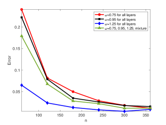
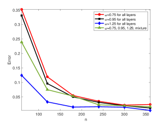
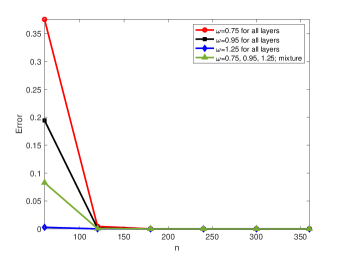
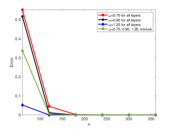
Figure 1: The clustering errors for $K=3$, $M=3$ (top left), $K=3$, $M=6$ (top right), $K=6$, $M=3$ (bottom left), and $K=6$, $M=6$ (bottom right). The number of nodes ranges from $n=60$ to $n=360$ with the increments of 60. The number of layers, $L=60$, is fixed for all panels. The lines with different colors represent the results for different values of $\omega$: $\omega=0.75$ (red); $\omega=0.95$ (black); $\omega=1.25$ (blue); $\omega=0.75,0.95,1.25$ (green). The errors are evaluated over 100 simulation runs.

In this section, we carry out a limited simulation study to illustrate the performance of our clustering method for finite values of $n$ and $L$. To this end, we investigate the effect of various combinations of model parameters on the clustering errors obtained by our algorithms. The proportion of misclassified layers (the between-layer clustering error) is evaluated as

$$\mbox{Err}(C,\widehat{C})=(2L)^{-1}\,\underset{\mathscr{P}_{M}\in\mathfrak{F}(M)}{\min}\|\widehat{C}-C\mathscr{P}_{M}\|_{F}^{2}$$ (38)

where $C,\widehat{C}\in\{0,1\}^{L\times M}$ are, respectively, the true and the estimated clustering matrices.

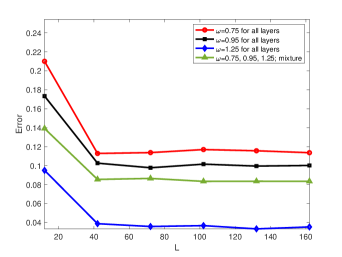
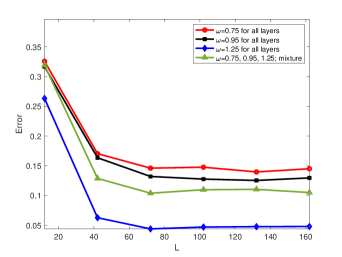
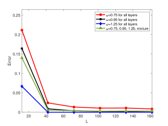
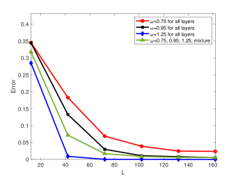
Figure 2: The clustering errors for $K=3$, $M=3$ (top left), $K=3$, $M=6$ (top right), $K=6$, $M=3$ (bottom left), and $K=6$, $M=6$ (bottom right). The number of layers ranges from $L=12$ to $L=162$ with the increments of 30. The number of nodes, $n=100$, is fixed for all panels. The lines with different colors represent the results for different values of $\omega$: $\omega=0.75$ (red); $\omega=0.95$ (black); $\omega=1.25$ (blue); $\omega=0.75,0.95,1.25$ (green). The errors are evaluated over 100 simulation runs.

In our simulations, we generate layer and node memberships as multinomial random variables, as it is described in Section 4.1, where $\pi_{k}=1/K$, $k\in[K]$, and $\varpi_{m}=1/M$, $m\in[M]$. The block probability matrices $B^{(l)}$ are generated as follows. First, elements of the diagonal and the lower halves of $B^{(l)}$ are generated as independent uniform random variables on the interval $[a,b]$, and the upper halves are obtained by symmetry. Subsequently, all non-diagonal elements of $B^{(l)}$ are multiplied by assortativity parameter $\omega>0$. When $\omega<1$ is small, the layer networks are assortative; when $\omega>1$ is large, they are disassortative; otherwise, they can be neither. We find the probability matrices $P^{(l)}$ using (1), and generate symmetric adjacency matrices $A^{(l)}$, $l=1,...,L$, with the lower halves obtained as independent Bernoulli variables $A^{(l)}_{i,j}\sim\mbox{Bernoulli}(P^{(l)}_{i,j})$, $1\leq j<i\leq n$. Finally, we set $A^{(l)}_{i,j}=A^{(l)}_{j,i}$ when $j>i$, and $A^{(l)}_{i,i}=0$ since diagonal elements are not available.

We apply Algorithms 3 and 4 to find the clustering matrix $\widehat{C}$. In Algorithm 3, the tuning parameter $\lambda$ is chosen empirically from synthetic networks as $\lambda=4\bar{\widehat{Q}}$ where $\bar{\widehat{Q}}$ is the average of the absolute values of entries of matrix $\widehat{Q}$ defined in (18).

We carry out simulations with $K=3$ or 6 and $M=3$ or 6. In our simulations, we choose $[a,b]=[0.3,0.8]$ and use three different values for $\omega$, $\omega=0.75$, 0.95, and 1.25. Specifically, we generate four types of multilayer networks: (i) a multilayer network whose all layers are generated using $\omega=0.75$; (ii) a multilayer network whose all layers are generated using $\omega=0.95$; (iii) a multilayer network whose all layers are generated using $\omega=1.25$; (iv) a multilayer network whose each one-third of layers corresponds to one of those three values of $\omega$ (a mixture of types (i), (ii), and (iii)).

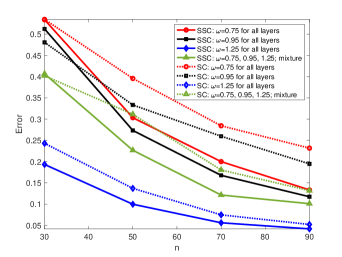
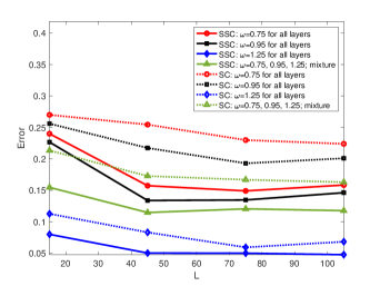
Figure 3: Comparison of clustering errors between Algorithm 4 (solid) and the method described in Pensky and Wang (2021) (dotted) for $K=3$, $M=3$. Left panel: $L=60$ and the number of nodes ranges from $n=30$ to $n=90$ with the increments of 20. Right panel: $n=80$ and the number of layers ranges from $L=15$ to $L=105$ with the increments of 30.

Figure 1 displays the between layer clustering errors for four types of multilayer networks with the fixed number of layers $L=60$, and $K=3$, $M=3$ (top left), $K=3$, $M=6$ (top right), $K=6$, $M=3$ (bottom left), and $K=6$, $M=6$ (bottom right). The number of nodes ranges from $n=60$ to $n=360$ with the increments of 60. Figure 2 displays the between layer clustering errors for four types of multilayer networks with the fixed number of nodes $n=100$, and $K=3$, $M=3$ (top left), $K=3$, $M=6$ (top right), $K=6$, $M=3$ (bottom left), and $K=6$, $M=6$ (bottom right). The number of layers ranges from $L=12$ to $L=162$ with the increments of 30.

Each of the panels presents all four scenarios for parameter $\omega$. It is easy to see that $\omega=1.25$ leads to the smallest and $\omega=0.75$ to the largest between-layer clustering errors. This is due to the fact that smaller values of $\omega$ lead to sparser networks, and the between-layer clustering error decreases when $n\rho_{n}$ grows. The latter shows that parameter $\omega$ does not act as a “signal-to-noise” ratio in the between-layer clustering, as it happens in community detection in the SBM. Indeed, if this were true, then the between layer clustering error would be smaller for $\omega=0.75$ than for $\omega=0.95$.

It is easy to see that, for a fixed value of $L$, the between layer clustering errors approach zero for all four types of networks as $n$ increases (since $\rho_{n}$ depends on the value of $\omega$ only and is fixed). On the other hand, when $n$ is fixed and $L$ grows, the between layer clustering errors decrease initially and then flattens. This agrees with the assessment of Pensky and Wang (2021) where the authors observed the similar phenomenon. Indeed, growing $L$ neither increases separation between subspaces, nor decreases the random deviations between the true vectors $\mathbf{x}^{(l)}$ and their estimated versions $\mathbf{y}^{(l)}$. Initial decrease in the error rate is due to initial decrease in the values of $\aleph_{w,K}$ in Assumption A5, the value of which flattens as $L$ grows. Also, as both figures show, the errors, for fixed $n$ and $L$, are larger for larger values of $K$ and $M$ (in all cases), which agrees with our theoretical assessments.

Figure 3 shows the results of comparison of the between layer clustering errors of Algorithm 4 and the technique described in Pensky and Wang (2021), which is based on the Spectral Clustering (SC). Since the algorithm used in Pensky and Wang (2021) is computationally very expensive as $n$ grows, we have compared the performances of these two methods using relatively small values of $n$. Specifically, Figure 3 illustrates the performances of the methods in two scenarios: fixed $L=60$ and the number of nodes ranging from $n=30$ to $n=90$ with the increments of 20 (left panel); fixed $n=80$ and the number of layers ranges from $L=15$ to $L=105$ with the increments of 30 (right panel). For both panels, $K=3$ and $M=3$. It is easy to see that, Algorithm 4 is competitive with the clustering method used in Pensky and Wang (2021). In fact, the former outperforms the latter in almost all cases.

6 A Real Data Example

In this section, we apply the proposed method to the Worldwide Food Trading Networks data collected by the Food and Agriculture Organization of the United Nations. The data have been described in De Domenico et al. (2015), and it is available at
https://www.fao.org/faostat/en/#data/TM. The data includes export/import trading volumes among 245 countries for more than 300 food items. In this multiplex network, layers represent food products, nodes are countries and edges at each layer represent import/export relationships of a specific food product among countries.

Table 1: List of three groups of food products obtained by Algorithm 4

	Food Products
Group 1	”Macaroni”, ”Pastry”, ”Rice, paddy (rice milled equivalent)”,
	”Rice, milled”, ”Cereals, breakfast”, ”Mixes and doughs”,
	”Food preparations, flour, malt extract”, ”Wafers”, ”Sugar nes”,
	”Sugar confectionery”, ”Nuts, prepared (exc. groundnuts)”,
	”Vegetables, preserved nes”, ”Juice, orange, single strength”,
	”Juice, fruit nes”, ”Fruit, prepared nes”, ”Beverages, non alcoholic”,
	”Beverages, distilled alcoholic”, ”Food wastes”, ”Coffee, green”,
	”Coffee, roasted”, ”Chocolate products nes”, ”Pepper (piper spp.)”,
	”Pet food”, ”Food prep nes”, ”Crude materials”
Group 2	”Flour, wheat”, ”Flour, maize”, ”Infant food”, ”Sugar refined”,
	”Oil, sunflower”, ”Waters,ice etc”, ”Meat, cattle, boneless (beef & veal)”,
	”Butter, cow milk”, ”Buttermilk, curdled, acidified milk”, ”Milk, whole dried”,
	”Milk, skimmed dried”, ”Cheese, whole cow milk”, ”Cheese, processed”,
	”Ice cream and edible ice”, ”Meat, pig sausages”, ”Meat, chicken”,
	”Meat, chicken, canned”, ”Margarine, short”
Group 3	”Wheat”, ”Maize”, ”Potatoes”, ”Potatoes, frozen”, ”Sugar Raw Centrifugal”,
	”Lentils”, ”Groundnuts, prepared”, ”Oil, olive, virgin”,
	”Chillies and peppers, green”, ”Vegetables, fresh nes”,
	”Vegetables, dehydrated”, ”Vegetables in vinegar”, ”Vegetables, frozen”,
	”Juice, orange, concentrated”, ”Apples”, ”Pears”, ”Grapes”,
	”Dates”, ”Fruit, fresh nes”, ”Fruit, dried nes”, ”Coffee, extracts”,
	”Tea”, ”Spices nes”, ”Oil, essential nes”, ”Cigarettes”

In our analysis we used data for the year 2018. As a pre-processing step, we remove low density layers and nodes. The original dataset contains 207 countries and 395 traded products. We choose the countries that are active in trading of at least 70% of products, reducing the number of countries to 130. To create a network for each product, we draw an edge between two countries if the export/import value of the product exceeds $10,000. After that, we choose the layers whose average degrees are larger than 10%, that is, layers with average degrees of at least 13. This reduces the number of layers to 68, so that the final multilayer network has 68 layers with 130 nodes in each layer.

Subsequently, we use Algorithm 4 to partition layers of the multiplex network (food products) into groups. For this purpose, we choose $K=5$ which is consistent with the number of continents (Africa, Americas, Asia, Europe, and Oceania) and can be considered as a natural partition of countries, although different groups of layers may have different communities. After experimenting with different values of $M$, we choose $M=3$ since it provides the most meaningful clustering results.

Table 1 represents the list of food products in the three resulting clusters. As is evident from Table 1, group 1 contains mostly cereals, stimulant crops, and derived products; group 2 consists mostly of animal products, and most products in group 3 are fruits, vegetables, and products derived from them (like tea or vegetable oil).

Table 2: List of three groups of food products obtained by ALMA

	Food Products
Group 1	”Pastry”, ”Sugar confectionery”, ”Fruit, prepared nes”,
	”Beverages, non alcoholic”, ”Beverages, distilled alcoholic”,
	”Food wastes”, ”Chocolate products nes”, ”Food prep nes”, ”Crude materials”
Group 2	”Cereals, breakfast”, ”Infant food”, ”Wafers”, ”Mixes and doughs”,
	”Food preparations, flour, malt extract”, ”Potatoes”, ”Potatoes, frozen”,
	”Oil, sunflower”, ”Chillies and peppers, green”, ”Vegetables, frozen”,
	”Apples”, ”Waters,ice etc”, ”Coffee, roasted”, ”Cigarettes”, ”Pet food”,
	”Meat, cattle, boneless (beef & veal)”, ”Butter, cow milk”,
	”Buttermilk, curdled, acidified milk”, ”Milk, whole dried”,
	”Milk, skimmed dried”, ”Cheese, whole cow milk”, ”Cheese, processed”,
	”Ice cream and edible ice”, ”Meat, pig sausages”, ”Meat, chicken”,
	”Meat, chicken, canned”, ”Margarine, short”
Group 3	”Wheat”, ”Flour, wheat”, ”Macaroni”, ”Rice, paddy (rice milled equivalent)”,
	”Rice, milled”, ”Maize”, ”Flour, maize”, ”Sugar Raw Centrifugal”,
	”Sugar refined”, ”Sugar nes”, ”Lentils”, ”Nuts, prepared (exc. groundnuts)”,
	”Groundnuts, prepared”, ”Oil, olive, virgin”, ”Vegetables, fresh nes”,
	”Vegetables, dehydrated”, ”Vegetables in vinegar”,
	”Vegetables, preserved nes”, ”Juice, orange, single strength”,
	”Juice, orange, concentrated”, ”Pears”, ”Grapes”, ”Dates”, ”Fruit, fresh nes”,
	”Fruit, dried nes”, ”Juice, fruit nes”, ”Coffee, green”, ”Coffee, extracts”,
	”Tea”, ”Pepper (piper spp.)”, ”Spices nes”, ”Oil, essential nes”

In order to study communities for each of the three groups of layers, we apply the bias-adjusted clustering algorithm of Lei and Lin (2021). Indeed, it is shown to be more robust than pure averaging of adjacency matrices since we cannot be sure that all layers of the network are assortative. Figure 4 confirms that communities are indeed different for different types of food layers. Indeed, for Group 1, community 1 mainly includes Middle East, South Asia and Australia, community 2 - Central and South America, community 3 - Africa, community 4 - former Soviet Union, community 5 - Western Europe and Indochina. For Group 2, community 1 is comprised of countries in Middle East and Northern and Central Africa, community 2 - Central and South America and some Central Asian Countries, community 3 - Southern and Central Africa, community 4 - Western Europe, community 5 - Canada, US, Asia and Australia. Finally, for Group 3, communities are much more mixed and scattered over the continents.

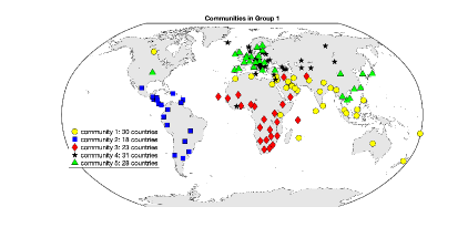
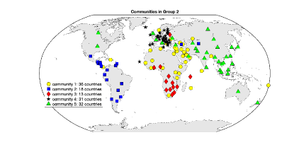
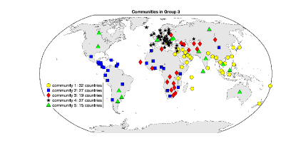
Figure 4: Trading communities of countries for products in groups 1,2 and 3.

As a comparison, we also carry out clustering of layers using the Alternating Minimization Algorithm (ALMA) introduced in Fan et al. (2022) for clustering a multiples network that follows the MMLSBM. ALMA is known to be competitive with TWIST (Jing et al. (2021)), another clustering method employed for the MMLSBM. The purpose of the comparison is to prove that, due to the flexibility of the DIMPLE model, it allows a better fit to the data than the MMLSBM.

Table 2 contains the list of food products in the three resulting groups obtained by ALMA with $K=5$ and $M=3$. We see that, similarly to the results in Table 1, most animal products are in group 2 and most fruits, vegetables, and derived products are classified in group 3. However, we do not see any dominant type of products in group 1 and the products do not seem to have meaningful relationships. Other possible values of $M$ don’t lead to meaningful groups either. Hence, the network does not seem to fit the MMLSBM well.

Therefore, based on results in Table 1 and Table 2, we can conclude that the DIMPLE model, with our proposed clustering method, is more suitable for this network.

7 Discussion

The present paper considers the DIverse MultiPLEx (DIMPLE) network model, introduced in Pensky and Wang Pensky and Wang (2021). However, while Pensky and Wang (2021) applied spectral clustering to the proxy of the adjacency tensor, this paper uses the SSC for identifying groups of layers with identical community structures. We provide algorithms for the between-layer clustering and formulate sufficient conditions, under which these algorithms lead to the strongly consistent clustering. Indeed, if the number of nodes is large enough, then the clustering error becomes zero with high probability.

The SSC has been applied to clustering single layer networks in Noroozi and Pensky (2022), Noroozi et al. (2021) and Noroozi et al. (2021). To the best of our knowledge, our paper offers the first application of the SSC to the Bernoulli multilayer network. While the weights in Algorithm 3 are obtained in a relatively conventional manner, our between-layer clustering Algorithm 4 is entirely original and very different from the one in Wang et al. (2016).

In addition, neither of Noroozi and Pensky (2022), Noroozi et al. (2021) and Noroozi et al. (2021) offer any evaluation of clustering errors. To the best of our knowledge, this paper is the first one to provide assessment of clustering precision of an SSC-based algorithm which is applied to a non-Gaussian network. Specifically, majority of papers provide theoretical guarantees for the sparse subspace clustering under the assumptions of spherical symmetry of the residuals and sufficient sampling density (see, e.g., Soltanolkotabi and Candes (2012), Soltanolkotabi et al. (2014), Wang and Xu (2016)). It is easy to observe that rotational invariance fails in the case of the Bernoulli random vectors. In addition, the assumption that the sampled vectors uniformly cover each of the subspaces may not be true either (for example, it does not hold for the MMLSBM). For this reason, our paper offers a completely original proof of the clustering precision of the SSC-based technique.

The present paper offers a strongly consistent between-layer clustering algorithm. In comparison, the spectral clustering Algorithm 1 of Pensky and Wang (2021) leads, with high probability, to the between layer clustering error of $O(K^{2}\,(n\rho_{n})^{-1})$. The latter results in a higher within-layer clustering error $R_{WL}^{(PW)}$. Indeed, assumptions in both papers are similar, and, with high probability, for some constants $C_{1}$ and $C_{2}$,

$$R_{WL}^{(PW)} \leq C_{1}\,\left(\frac{MK^{4}\log(L+n)}{n\,\rho_{n}\,L}+\frac{MK^{6}}{n\,\rho_{n}}\right)$$

(39)

$$R_{WL} \leq C_{2}\,\left(\frac{MK^{4}\log(L+n)}{n\,\rho_{n}\,L}\ +\frac{K^{4}}{n^{2}}\right)$$

where the second expression in (39) is a repetition of formula (37). While the first terms in the expressions of $R_{WL}^{(PW)}$ and $R_{WL}$ coincide, the second term in $R_{WL}^{(PW)}$ is significantly larger than the one in $R_{WL}$. Indeed, the second term in $R_{WL}^{(PW)}$ results from the between layer clustering error of $O(K^{2}\,(n\rho_{n})^{-1})$. On the contrary $K^{4}\,n^{-2}$ in (37) is due to smaller order terms.

Clustering methodology in this paper has a number of advantages. Not only is it strongly consistent with high probability when the number of nodes is large, but also competitive with (and often more precise than) the spectral clustering in Pensky and Wang (2021). In addition, the algorithm of Pensky and Wang (2021) requires SVD of $n(n-1)/2\times L$ matrix, which is challenging for large $n$, while in our case the SVD is applied to $L\times L$ matrix. Hence, the SSC-based technique allows to handle much larger networks. Moreover, the most time consuming part of the algorithm, finding the weight matrix, is perfectly suitable for application of parallel computing which can drastically reduce the computational time.

Appendix A Proofs

A.1 Proof of Self-Expressiveness property under the separation condition

Proof of Theorem 1 relies on the fact that the subspaces ${\cal S}_{m}$, $m=1,...,M$, corresponding to different types of layers do not have large intersections. Specifically, we prove the following statement from which the validity of Theorem 1 will readily follow.

Proposition 1.

Let Assumptions A1, A2, A3 and A5 hold. Let $L_{m}$ and $n_{k}^{(m)}$be, respectively, the number of layers of type $m$ and the number of nodes in the $k$-th community in the group of layers of type $m$, where $L_{m}$ and $n_{k}^{(m)}$ satisfy condition (27). Assume, in addition, that there exists $\tau\equiv\tau_{n,K}\in(0,1)$ such that for any arbitrary vectors $\mathbf{x}\in{\cal S}_{m}$ and $\mathbf{x}^{\prime}\in{\cal S}_{m^{\prime}}$, where $m\neq m^{\prime}$, one has $|\mathbf{x}^{T}\mathbf{x}^{\prime}|\leq\tau\,\|\mathbf{x}\|\,\|\mathbf{x}^{\prime}\|$. Let $t>0$ and $\delta=\delta_{n,K,t}$ be defined in (29) where $C_{t,\delta}$ is a constant that depends only on $t$ and constants in Assumptions A1, A2, A3 and A5, and condition (27).

Let $\widehat{W}$ be a solution of problem (19) with $\lambda=\lambda_{n,K}$ such that

$$\lambda_{n,K}\leq(4\,\aleph_{w,K})^{-1},\quad\lim_{n\to\infty}\frac{(\delta_{n,K,t}+\tau_{n,K})(1+\aleph_{w,K})}{\lambda_{n,K}}=0$$ (40)

where $\aleph_{w,K}$ is defined in Assumption A5. If $\displaystyle{\max_{1\leq l\leq L}\|\mathbf{y}^{(l)}-\mathbf{x}^{(l)}\|\leq\delta}$ and $n$ is large enough, then, matrix $\widehat{W}$ (and, consequently, $\widehat{\widetilde{W}}$) satisfies the SEP.

Proof of Proposition 1.
Let matrices $Q,X\in{\mathbb{R}}^{n^{2}\times L}$ and $\widehat{Q},Y\in{\mathbb{R}}^{n^{2}\times L}$ be defined in (22) and (18), respectively. Choose an arbitrary $l_{0}\in[L]$ and, without loss of generality, assume that $c(l_{0})=1$, i.e. $\mathbf{x}^{(l_{0})}\in{\cal S}_{1}$. Denote $\mathbf{x}=\mathbf{x}^{(l_{0})}$, $\mathbf{y}=\mathbf{y}^{(l_{0})}$, $\widetilde{\cal S}={\cal S}_{1}$ and $\widetilde{\widetilde{\cal S}}={\cal S}_{2}\cup\ldots\cup{\cal S}_{M}$, and present the remainder of matrix $X$ (i.e., $X$ with $X(:,l_{0})$ removed) as $[\widetilde{X}\,|\,\widetilde{\widetilde{X}}]$. Here, $\widetilde{X}$ and $\widetilde{\widetilde{X}}$ are portions of $X$ with $X(:,l_{0})$ removed, that correspond to $\widetilde{\cal S}$ and $\widetilde{\widetilde{S}}$, respectively. With some abuse of notations, we denote $X$ with $X(:,l_{0})$ removed by $X$ again, i.e., $X=[\widetilde{X}\,|\,\widetilde{\widetilde{X}}]$.

Denote $Z=Y-X$, $\mathbf{z}^{(l)}=Z(:,l)$ and $\mathbf{z}=\mathbf{z}^{(l_{0})}=\mathbf{y}-\mathbf{x}$, so that

$$\widetilde{Y}=\widetilde{X}+\widetilde{Z},\quad\widetilde{\widetilde{Y}}=\widetilde{\widetilde{X}}+\widetilde{\widetilde{Z}},\quad\mathbf{y}=\mathbf{x}+\mathbf{z}$$

Let $\mathbf{w}=[\widetilde{\mathbf{w}}\,|\,\widetilde{\widetilde{\mathbf{w}}}]$ be the solution of problem (19) for $l=l_{0}$. Then, (19) implies that

$$\|\mathbf{y}-\widetilde{Y}\widetilde{\mathbf{w}}-\widetilde{\widetilde{Y}}\widetilde{\widetilde{\mathbf{w}}}\|^{2}+2\lambda\|\widetilde{\mathbf{w}}\|_{1}+2\lambda\|\widetilde{\widetilde{\mathbf{w}}}\|_{1}\leq\|\mathbf{y}-\widetilde{Y}\widetilde{\mathbf{w}}\|^{2}+2\lambda\|\widetilde{\mathbf{w}}\|_{1}$$

By simplifying the inequality, obtain

$$\Delta\overset{def}{=}\|\widetilde{\widetilde{Y}}\widetilde{\widetilde{\mathbf{w}}}\|^{2}-2\langle\mathbf{y}-\widetilde{Y}\widetilde{\mathbf{w}},\widetilde{\widetilde{Y}}\widetilde{\widetilde{\mathbf{w}}}\rangle+\lambda\|\widetilde{\widetilde{\mathbf{w}}}\|_{1}\leq 0$$ (41)

Note that the Cauchy-Schwarz inequality and Assumption A5 yield

$$\langle\mathbf{y}-\widetilde{Y}\widetilde{\mathbf{w}},\widetilde{\widetilde{Y}}\widetilde{\widetilde{\mathbf{w}}}\rangle\leq \tau\|\mathbf{x}-\widetilde{X}\widetilde{\mathbf{w}}\|\|\widetilde{\widetilde{X}}\widetilde{\widetilde{\mathbf{w}}}\|+\|\mathbf{z}-\widetilde{Z}\widetilde{\mathbf{w}}\|\|\widetilde{\widetilde{X}}\widetilde{\widetilde{\mathbf{w}}}\|$$

$$+ \|\mathbf{x}-\widetilde{X}\widetilde{\mathbf{w}}\|\|\widetilde{\widetilde{Z}}\widetilde{\widetilde{\mathbf{w}}}\|+\|\mathbf{z}-\widetilde{Z}\widetilde{\mathbf{w}}\|\|\widetilde{\widetilde{Z}}\widetilde{\widetilde{\mathbf{w}}}\|$$

Moreover,

$$\|\mathbf{z}-\widetilde{Z}\widetilde{\mathbf{w}}\|\leq[\|\widetilde{\mathbf{w}}\|_{1}+1]\delta;\quad\|\widetilde{\widetilde{Z}}\widetilde{\widetilde{\mathbf{w}}}\|\leq\|\widetilde{\widetilde{\mathbf{w}}}\|_{1}\delta;\quad\|\mathbf{x}-\widetilde{X}\widetilde{\mathbf{w}}\|\leq\|\widetilde{\mathbf{w}}\|_{1}+1$$

Since $\|\widetilde{\widetilde{Y}}\widetilde{\widetilde{\mathbf{w}}}\|^{2}\geq 0.5\,\|\widetilde{\widetilde{X}}\widetilde{\widetilde{\mathbf{w}}}\|^{2}-\|\widetilde{\widetilde{Z}}\widetilde{\widetilde{\mathbf{w}}}\|^{2}$, obtain

$$\Delta\geq \left[0.5\,\|\widetilde{\widetilde{X}}\widetilde{\widetilde{\mathbf{w}}}\|^{2}-2(\tau+\delta)(\|\widetilde{\mathbf{w}}\|_{1}+1)\|\widetilde{\widetilde{X}}\widetilde{\widetilde{\mathbf{w}}}\|\right]$$ (42)

$$+\|\widetilde{\widetilde{\mathbf{w}}}\|_{1}\left[\lambda-\delta-2(\|\widetilde{\mathbf{w}}\|_{1}+1)\delta(1+\delta)\right]$$

To find an upper bound for $(\|\widetilde{\mathbf{w}}\|_{1}+1)$, consider $\widetilde{\mathbf{w}}_{*}$, the solution of exact problem, that is $\mathbf{x}=\widetilde{X}\widetilde{\mathbf{w}}_{*}$. By Assumption A6, there exists a sub-matrix $\widetilde{X}_{*}\in{\mathbb{R}}^{n^{2}\times(K-1)^{2}}$ of $\widetilde{X}$, such that $\mathbf{x}=\widetilde{X}_{*}{\mathbf{w}}_{*}$ and $\|\mathbf{w}_{*}\|_{1}\leq\aleph_{w,K}$. Let $\widetilde{Y}_{*}$ be the portion of $\widetilde{Y}$ corresponding to $\widetilde{X}_{*}$ and $\widetilde{Z}_{*}=\widetilde{Y}_{*}-\widetilde{X}_{*}$. Since $\|\mathbf{y}-\widetilde{Y}\mathbf{w}_{*}\|^{2}=\|\mathbf{z}-\widetilde{Z}\mathbf{w}_{*}\|^{2}$, derive

$$\|\mathbf{y}-\widetilde{Y}\mathbf{w}_{*}\|^{2}+2\lambda\|\mathbf{w}_{*}\|_{1}\leq\delta^{2}\left[\|\mathbf{w}_{*}\|_{1}+1\right]^{2}+2\lambda\|\mathbf{w}_{*}\|_{1}$$ (43)

Note that, since $\mathbf{w}_{*}$ is not an optimal solution, one has

$$\|\mathbf{y}-\widetilde{Y}\mathbf{w}_{*}\|^{2}+2\lambda\|\mathbf{w}_{*}\|_{1}\geq\|\mathbf{y}-\widetilde{Y}\widetilde{\mathbf{w}}-\widetilde{\widetilde{Y}}\widetilde{\widetilde{\mathbf{w}}}\|^{2}+2\lambda\|\widetilde{\mathbf{w}}\|_{1}+2\lambda\|\widetilde{\widetilde{\mathbf{w}}}\|_{1}\geq 2\lambda\|\widetilde{\mathbf{w}}\|_{1}$$

Thus, $\|\widetilde{\mathbf{w}}\|_{1}+1\leq(\|\mathbf{w}_{*}\|_{1}+1)+\|\mathbf{y}-\widetilde{Y}\mathbf{w}_{*}\|^{2}/(2\lambda)$, so that

$$\|\widetilde{\mathbf{w}}\|_{1}+1\leq(1+\aleph_{w,K})+0.5\,\delta^{2}\,(1+\aleph_{w,K})^{2}/\lambda$$ (44)

Then, using (42) and (44), due to $\|\widetilde{\widetilde{X}}\widetilde{\widetilde{\mathbf{w}}}\|\leq\|\widetilde{\widetilde{\mathbf{w}}}\|_{1}$, obtain

$$\Delta\geq \frac{1}{2}\,\|\widetilde{\widetilde{X}}\widetilde{\widetilde{\mathbf{w}}}\|^{2}$$

$$+\|\widetilde{\widetilde{\mathbf{w}}}\|_{1}\left[\lambda-\delta-2\,(1+\aleph_{w,K})\left(1+\frac{1}{2}\delta^{2}(1+\aleph_{w,K})/\lambda\right)(2\delta+2\tau+\delta^{2})\right]$$

Now, observe that, due to condition (40), $\delta<1$ and $\delta^{2}(1+\aleph_{w,K})/\lambda$ tends to zero. Hence, for $n$ large enough, arrive at

$$\Delta\geq\frac{1}{2}\|\widetilde{\widetilde{X}}\widetilde{\widetilde{\mathbf{w}}}\|^{2}+\lambda\|\widetilde{\widetilde{\mathbf{w}}}\|_{1}\left[1-\frac{\delta}{\lambda}-\frac{12\,(\delta+\tau)(1+\aleph_{w,K})}{\lambda}\right]>0$$

unless $\widetilde{\widetilde{\mathbf{w}}}=0$. Since, by (41), $\Delta\leq 0$, one has $\widetilde{\widetilde{\mathbf{w}}}=0$ and the SEP holds.

In order to complete the proof, we need to show that there exists $\lambda$ which is not too large, so the optimization problem (19) for $l=l_{0}$ has a non-zero solution. If we show that, for some $\mathbf{w}\neq 0$, the objective function is smaller than that for $\mathbf{w}\equiv 0$, then (19) for $l=l_{0}$ yields a non-zero solution. To this end, we find a sufficient condition such that $\|\mathbf{y}-\widetilde{Y}\mathbf{w}_{*}\|^{2}+2\lambda\|\mathbf{w}_{*}\|_{1}\leq\|\mathbf{y}\|^{2}=1$ holds. It follows from (43) and Assumption A6 that

$$\|\mathbf{y}-\widetilde{Y}\mathbf{w}_{*}\|^{2}+2\lambda\|\mathbf{w}_{*}\|_{1}\leq\delta^{2}(1+\aleph_{w,K})^{2}+2\lambda\aleph_{w,K}$$

Hence,

$$\delta^{2}\,(1+\aleph_{w,K})^{2}+2\lambda\aleph_{w,K}\leq 1$$

is sufficient for $\mathbf{w}\neq 0$. By condition (40), one has $\delta\,(1+\aleph_{w,K})\to 0$ as $n\rightarrow\infty$, so that for $n$ large enough, $\delta\,(1+\aleph_{w,K})\leq 1/2$. Therefore, $2\lambda\aleph_{w,K}\leq 1/2$ is sufficient for $\mathbf{w}\neq 0$, which is equivalent to the first inequality in (40). The latter completes the proof.

A.2 Proof of Theorem 1

In order to prove that Theorem 1 holds, we show that, under assumptions of Theorem 1, (27) is true and that $\tau_{n,K}\leq\mathbb{C}K^{2}\,n^{-1}\,\log n$ in Proposition 1. Let $\widehat{L}_{m}$ and $\hat{n}_{k}^{(m)}$ be defined in (26). Then, the following statements are valid.

Lemma 2.

Let Assumption A4 hold. Let $t>0$ satisfy condition (31). Then, there exists a set $\bar{\Omega}_{t1}$ with

$${\mathbb{P}}(\Omega_{t1})\geq 1-2L^{-t}-2KM\,n^{-t}$$

such that, for $\omega\in{\Omega}_{t1}$, one has simultaneously

$$\frac{\underline{c}_{\varpi}\,L}{2\,M}\leq\widehat{L}_{m}\leq\frac{3\,\bar{c}_{\varpi}\ L}{2\,M},\quad{\rm and}\quad\bigcap_{m=1}^{M}\bigcap_{k=1}^{K}\left\{\omega:\frac{\underline{c}_{\pi}\,n}{2\,K}\leq\hat{n}_{k}^{(m)}\leq\frac{3\,\bar{c}_{\pi}\ n}{2\,K}\right\}$$ (45)

Apply the following lemma, proved later in Section A.5, which ensures the upper bound $\displaystyle\max_{l}\,\|\mathbf{y}^{(l)}-\mathbf{x}^{(l)}\|\leq\delta_{n,K,t}$ in Proposition 1.

Lemma 3.

Let Assumptions of Theorem 1 hold and $t>0$ satisfies condition (31). Let $\mathbf{q}^{(l)}$ and $\hat{\mathbf{q}}^{(l)}$ be defined in (15) and (18), respectively. Let matrices $Q,\widehat{Q}\in{\mathbb{R}}^{n^{2}\times L}$ be defined in (22) and (18), respectively. Then,

$$\min_{l}\|\mathbf{q}^{(l)}\|\geq\widetilde{C}_{0}C_{\sigma,0}\,\underline{C}\,K^{-1/2}\,n\,\rho_{n},\quad\max_{l}\|\mathbf{q}^{(l)}\|\leq\widetilde{\widetilde{C}}_{0}\,\bar{C}\,K^{-1/2}\,n\,\rho_{n}$$ (46)

Moreover, there exists a set $\Omega_{t2}$ such that ${\mathbb{P}}(\Omega_{t2})\geq 1-Ln^{-t}$, and for $\omega\in\Omega_{t2}$, one has

$$\max_{l}\ \|\hat{\mathbf{q}}^{(l)}-\mathbf{q}^{(l)}\|/\|\mathbf{q}^{(l)}\|\leq C_{t,\rho,\sigma}\,K/\sqrt{n\rho_{n}}$$ (47)

where $C_{t,\rho,\sigma}$ depends only on $t$ and constants in Assumptions A1–A5.

In addition, the following lemma provides an upper bound on $\tau_{n,K}$ in Proposition 1.

Lemma 4.

Let Assumption A4 hold, and $Z_{j,k}^{(m)}$, $k\in[K]$, $j\in[n]$, $m\in[M]$, be generated according to (21). Let $t>0$ satisfy condition (31). Then, there exists a set $\Omega_{t3}$ with

$${\mathbb{P}}(\Omega_{t3})\geq 1-2L^{-t}-2KM(M+1)\,n^{-t}$$

such that, for $\omega\in\Omega_{t3}$, and for any arbitrary vectors $\mathbf{x}\in{\cal S}_{m}$ and $\mathbf{x}^{\prime}\in{\cal S}_{m^{\prime}}$, where $m\neq m^{\prime}$, one has $|\mathbf{x}^{T}\mathbf{x}^{\prime}|\leq\tau\,\|\mathbf{x}\|\,\|\mathbf{x}^{\prime}\|$ with

$$\tau\equiv\tau_{n,K}\leq 2\,(\sqrt{2}+3/\underline{c}_{\pi})^{2}\,t\,K^{2}\,n^{-1}\,\log n$$ (48)

It is easy to show that, for any $l\in[L]$, one has $\|\mathbf{z}^{(l)}\|=\|\mathbf{y}^{(l)}-\mathbf{x}^{(l)}\|\leq 2\|\hat{\mathbf{q}}^{(l)}-\mathbf{q}^{(l)}\|/\|\mathbf{q}^{(l)}\|$. Hence, Lemma 3 implies that, for $\delta\equiv\delta_{n,K,t}$ defined in (29), one has

$${\mathbb{P}}\left\{\max_{1\leq l\leq L}\|\mathbf{z}^{(l)}\|\leq\delta\right\}\geq 1-Ln^{-t}$$ (49)

Now, in order to apply Proposition 1, it remains to show that condition (30) implies (40). For this purpose, note that, since columns of matrix $X$ have unit norms, one has $\aleph_{w,K}\geq 1$ in A5 and, hence, (40) implies that $\delta_{n,K,t}/\lambda_{n,K}\to 0$ as $n\to\infty$. The latter furthermore yields that $n^{-1}\,K^{2}\,\log n\to 0$, so that $\tau_{n,K}=o(\delta_{n,K,t})$ as $n\to\infty$, where $\tau_{n,K}$ and $\delta_{n,K,t}$ are defined in (48) and (29), respectively. This completes the proof.

A.3 Proof of Theorem 2

Let $\widehat{W}$ be the matrix of weights and $\Omega_{t}$ be the set in Theorem 1, so that $\Omega_{t}$ is exactly the set where SEP holds. Note that Algorithm 4 allows the situation where $\widetilde{M}<M$. However, if the SEP holds, then no two network layers in different clusters can be a part of the same connected component, and hence, $\widetilde{M}\geq M$.

Consider a clustering function $\phi:[L]\rightarrow[\widetilde{M}]$ and the corresponding clustering matrix $\Phi\in\{0,1\}^{L\times\widetilde{M}}$, which partitions $L$ layers into $\widetilde{M}\geq M$, disconnected components. Due to SEP, some of the vectors that belong to different clusters, according to $\phi$, belong to the same cluster, according to $c$. On the other hand, if two vectors belong to different clusters according to $c$, they belong to different clusters according to $\phi$. That is, for $l_{1},l_{2}=1,\ldots,L$, $l_{1}\neq l_{2}$, one has

$$\phi(l_{1})=\phi(l_{2})\,\Longrightarrow\,c(l_{1})=c(l_{2}),\quad c(l_{1})\neq c(l_{2})\,\Longrightarrow\,\phi(l_{1})\neq\phi(l_{2})$$ (50)

Hence, if $\widetilde{M}=M$, then $\phi=c$.

Let $\widetilde{M}>M$. Then, due to (50), one can partition $\widetilde{M}$ clusters into $M$ groups. Let $\theta:[\widetilde{M}]\rightarrow[M]$ be such clustering function, and $\Theta$ be the corresponding clustering matrix. Then, for $\omega\in\Omega_{t}$, SEP holds and $C=\Phi\Theta$. Observe that $\theta(\widetilde{m}_{1})=\theta(\widetilde{m}_{2})$ if $c(l_{i})=c(l_{j})$ for all $l_{i},l_{j}$ with $\phi(l_{i})=\widetilde{m}_{1}$ and $\phi(l_{j})=\widetilde{m}_{2}$, where $l_{i},l_{j}=1,\ldots,L,$ and $\widetilde{m}_{1},\widetilde{m}_{2}=1,\ldots,\widetilde{M}$. To prove the theorem, we use the following statement.

Lemma 5.

Let Assumptions A1 - A5 hold and $K^{2}/(n\rho_{n})\to 0$ as $n\to\infty$. Then, if $\omega\in\Omega_{t}$, for some positive constant $\check{C}$, one has

$$|(\mathbf{x}^{(l_{1})})^{T}\mathbf{x}^{(l_{2})}| \geq\check{C}\quad\text{if}\quad c(l_{1})=c(l_{2});$$

(51)

$$|(\mathbf{x}^{(l_{1})})^{T}\mathbf{x}^{(l_{2})}| \leq\tau_{n,K}\quad\text{if}\quad c(l_{1})\neq c(l_{2})$$ (52)

Moreover, for $\omega\in\Omega_{t}$ and $n$ large enough

$$\min_{\begin{subarray}{c}l_{1},l_{2}\\ c(l_{1})=c(l_{2})\end{subarray}}|(\mathbf{y}^{(l_{1})})^{T}\mathbf{y}^{(l_{2})}|\geq\check{C}/2,$$

$$\max_{\begin{subarray}{c}l_{1},l_{2}\\ c(l_{1})\neq c(l_{2})\end{subarray}}|(\mathbf{y}^{(l_{1})})^{T}\mathbf{y}^{(l_{2})}|\leq\tau_{n,K}+2\delta_{n,K,t}$$

Consider matrices $\Upsilon,\widehat{\Upsilon}\in{\mathbb{R}}^{L\times L}$ with elements

$$\Upsilon_{l_{1},l_{2}}=|(\mathbf{x}^{(l_{1})})^{T}\mathbf{x}^{(l_{2})}|,\quad\widehat{\Upsilon}_{l_{1},l_{2}}=|(\mathbf{y}^{(l_{1})})^{T}\mathbf{y}^{(l_{2})}|,\quad l_{1},l_{2}=1,\ldots,L$$

Denote $D_{\Phi}=(\Phi)^{T}\Phi$ and define matrices $\widetilde{\Upsilon},\widehat{\widetilde{\Upsilon}}\in{\mathbb{R}}^{\widetilde{M}\times\widetilde{M}}$

$$\widetilde{\Upsilon}=(D_{\Phi})^{-1/2}\Phi^{T}\Upsilon\Phi(D_{\Phi})^{-1/2},\quad\widehat{\widetilde{\Upsilon}}=(D_{\Phi})^{-1/2}\Phi^{T}\widehat{\Upsilon}\Phi(D_{\Phi})^{-1/2},$$

Then, due to (33), by Lemma 5, for $\widetilde{m}_{1},\widetilde{m}_{2}=1,\ldots,\widetilde{M}$, $\widetilde{\Upsilon}_{\widetilde{m}_{1},\widetilde{m}_{2}}\geq\check{C}$ if $\theta(\widetilde{m}_{1})=\theta(\widetilde{m}_{2})$, and $\widetilde{\Upsilon}_{\widetilde{m}_{1},\widetilde{m}_{2}}\leq\tau_{n,K}$ if $\theta(\widetilde{m}_{1})\neq\theta(\widetilde{m}_{2})$. Also, for $\omega\in\Omega_{t}$, one has $\widehat{\widetilde{\Upsilon}}_{\widetilde{m}_{1},\widetilde{m}_{2}}\geq{\check{C}}/2$ if $\theta(\widetilde{m}_{1})=\theta(\widetilde{m}_{2})$, and $\widehat{\widetilde{\Upsilon}}_{\widetilde{m}_{1},\widetilde{m}_{2}}\leq\tau_{n,K}+2\delta_{n,K,t}$ if $\theta(\widetilde{m}_{1})\neq\theta(\widetilde{m}_{2})$.

Now, consider matrices $G,\widehat{G}\in\{0,1\}^{\widetilde{M}\times\widetilde{M}}$ with

$$G_{\widetilde{m}_{1},\widetilde{m}_{2}}=I(\theta(\widetilde{m}_{1})=\theta(\widetilde{m}_{2})),\,\,\,\widehat{G}_{\widetilde{m}_{1},\widetilde{m}_{2}}=I(|\widehat{\widetilde{\Upsilon}}_{\widetilde{m}_{1},\widetilde{m}_{2}}|\geq T),\,\,\,\widetilde{m}_{1},\widetilde{m}_{2}=1,\ldots,\widetilde{M}$$

Then, $G=\Theta\Theta^{T}$. Moreover, if $n$ is large enough, then $\tau_{n,K}+2\delta_{n,K,t}<T<{\check{C}}/2$, whenever $T$ satisfies conditions (33). Consequently, $\widehat{G}=G$ for $\omega\in\Omega_{t}$ and hence, spectral clustering of $\widehat{G}$ correctly recovers $M$ clusters given by $\Theta$.

A.4 Proof of Theorem 3

The proof of this theorem is very similar to the proof of Theorem 3 in Pensky and Wang (2021). In this proof, same as before, we denote by $\mathbb{C}$ an absolute constant which can be different at different instances. Consider tensors $\mathbf{G}\in{\mathbb{R}}^{n\times n\times L}$ and $\mathbf{H}=\mathbf{G}\times_{3}(CD_{c}^{-1/2})^{T}\in{\mathbb{R}}^{n\times n\times M}$ with layers, respectively, $G^{(l)}=\mathbf{G}(:,:,l)$ and $H^{(m)}=\mathbf{H}(:,:,m)$ of the forms

$$G^{(l)}=(P^{(l)})^{2},\quad H^{(m)}=L_{m}^{-1/2}\,\sum_{c(l)=m}\,G^{(l)},\quad l\in[L],\ m\in[M]$$ (54)

In order to assess $R_{WL}$, one needs to examine the spectral structure of matrices $H^{(m)}$ and their deviation from the sample-based versions $\widehat{H}^{(m)}=\widehat{\mathbf{H}}(:,:,m)$. We start with the first task.

It follows from (3) and (5) that

$$H^{(m)}=U_{z}^{(m)}\,\bar{Q}_{D}^{(m)}\,(U_{z}^{(m)})^{T}\quad\mbox{with}\quad\bar{Q}_{D}^{(m)}=L_{m}^{-1/2}\,\sum_{c(l)=m}\,\left(B_{D}^{(l)}\right)^{2}$$ (55)

Since all eigenvalues of $(B_{D}^{(l)})^{2}$ are positive, applying the Theorem in Complement 10.1.2 on page 327 of Rao and Rao (1998) and Assumptions A1–A5, obtain that

$$\sigma_{\min}(H^{(m)}) =\sigma_{K}\left(\bar{Q}_{D}^{(m)}\right)\geq L_{m}^{-1/2}\,\sum_{c(l)=m}\sigma_{K}\left((B_{D}^{(l)})^{2}\right)$$

$$\geq L_{m}^{-1/2}\,\left(\min_{k}(\hat{n}_{k}^{(m)})\right)^{2}\ \rho_{n}^{2}\,\sum_{c(l)=m}\sigma_{K}\left((B_{0}^{(l)})^{2}\right)$$

$$\geq\mathbb{C}\,n^{2}\,\rho_{n}^{2}\,K^{-2}\,\sqrt{LM^{-1}}$$ (56)

Note that the Euclidean separation $\gamma_{m}$ of rows of $U_{H}^{(m)}$ is the same as the Euclidean separation of rows of $U_{z}^{(m)}$, and $\displaystyle\gamma_{m}^{2}\geq 2(\min_{k}(\hat{n}_{k}^{(m)}))^{-1}\geq\mathbb{C}K/n$ for $\omega\in\Omega_{t}$.

Therefore, by Lemma 9 of Lei and Lin (2021), derive that the total number of clustering errors $\Delta$ within all layers is bounded as

$$\Delta\leq\mathbb{C}\,\frac{n}{K}\,\sum_{m=1}^{M}\,\left\|\sin\Theta\left(\widehat{U}_{\widehat{H}}^{(m)},U_{H}^{(m)}\right)\right\|^{2}_{F}$$

Using Davis-Kahan theorem and formula (56), obtain

$$\left\|\sin\Theta\left(\widehat{U}_{\widehat{H}}^{(m)},U_{H}^{(m)}\right)\right\|^{2}_{F}\leq\frac{4K\|\widehat{H}^{(m)}-H^{(m)}\|^{2}}{\sigma^{2}_{\min}(H^{(m)})}\leq\mathbb{C}\,\frac{K^{5}M\,\|\widehat{H}^{(m)}-H^{(m)}\|^{2}}{n^{4}\rho_{n}^{4}L}$$

where we use $\mathbb{C}$ for different constants that depend on the constants in Assumptions A1-A5. Combination of the last two inequalities yields that the total number of clustering errors within all layers is bounded by

$$\Delta\leq\mathbb{C}\,\frac{K^{4}M}{n^{3}\rho_{n}^{4}L}\,\sum_{m=1}^{M}\,\|\widehat{H}^{(m)}-H^{(m)}\|^{2}$$ (57)

Recall that $H^{(m)}=[\mathbf{G}\times_{3}\Psi^{T}](:,:,m)$ and $\widehat{H}^{(m)}=[\widehat{\mathbf{G}}\times_{3}\widehat{\Psi}^{T}](:,:,m)$. Since, by Theorem 2, for $\omega\in\Omega_{t}$ one has $\widehat{\Psi}=\Psi$, obtain that

$$\|\widehat{H}^{(m)}-H^{(m)}\|^{2}\leq L_{m}^{-1}\left\|\bar{\widehat{G}}^{(m)}-\bar{G}^{(m)}\right\|^{2}$$

where

$$\bar{G}^{(m)}=\displaystyle\sum_{c(l)=m}G^{(l)}=\sqrt{L_{m}}\,H^{(m)},\quad\bar{\widehat{G}}^{(m)}=\sqrt{L_{m}}\,[\widehat{\mathbf{G}}\times_{3}\Psi^{T}](:,:,m)=\displaystyle\sum_{c(l)=m}\widehat{G}^{(l)}$$

use the following lemma that modifies upper bounds in Lei and Lin (2021) in the absence of the sparsity assumption $\rho_{n}n\leq\mathbb{C}$:

Lemma 6.

Let Assumptions A1–A5 hold, $G^{(l)}=(P^{(l)})^{2}$ and $\widehat{G}^{(l)}=(A^{(l)})^{2}-\mbox{diag}(A^{(l)}{\bf 1})$, where $c(l)=m$, $l=1,...,\tilde{L}$. Let

$$G=\sum_{l=1}^{\tilde{L}}\,G^{(l)},\quad\widehat{G}=\sum_{l=1}^{\tilde{L}}\,\widehat{G}^{(l)}$$

Then, for any $t>0$, there exists a constant $\widetilde{C}$ that depends only on $t$ and constants in Assumptions A1–A5, and $\widetilde{C}_{t,\epsilon}$ which depends only on $t$ and $\epsilon$ in Algorithm 2, such that one has

$${\mathbb{P}}\left\{\|\widehat{G}-G\|^{2}\leq\widetilde{C}\left[\rho_{n}^{3}n^{3}\tilde{L}\log(\tilde{L}+n)+\rho_{n}^{4}n^{2}\tilde{L}^{2}\right]\right\}\geq 1-\widetilde{C}_{t,\epsilon}(\tilde{L}+n)^{1-t}$$ (58)

Applying Lemma 6 with $\tilde{L}=L_{m}$, obtain that there exists a set $\Omega_{t4}$, with

$${\mathbb{P}}(\Omega_{t4})\geq 1-\widetilde{C}_{t,\epsilon}n^{1-t},$$

and for $\omega\in\Omega_{t4}$, one has

$$\|\widehat{H}^{(m)}-H^{(m)}\|^{2}\leq\mathbb{C}\,[\rho_{n}^{3}n^{3}\,\log(L+n)+\rho_{n}^{4}\,n^{2}L/M]$$ (59)

To complete the proof, combine formulas (57) and (59), set $\tilde{\Omega}_{t}=\Omega_{t}\cap\Omega_{t4}$ and recall that $R_{WL}=\Delta/(Mn)$ and $n\rho_{n}\geq C_{\rho}\log n$.

A.5 Proofs of supplementary statements

Proof of Lemma 1. First, we prove part (a). Recall that, for $l$ with $c(l)=m$, by formula (15), one has

$$\mathbf{q}^{(l)}=\rho_{n}\,(\widetilde{U}^{(m)}\otimes\widetilde{U}^{(m)})\left(\sqrt{D^{(m)}}\otimes\sqrt{D^{(m)}}\right)\mathbf{b}_{0}^{(l)}$$ (60)

Since ${\cal B}_{0}$ is a full rank matrix, one can present $\mathbf{b}_{0}^{(l_{0})}$ as $\mathbf{b}_{0}^{(l_{0})}={\cal B}_{0}\mathbf{w}$ for some vector $\mathbf{w}$. Note that, although vectors $\mathbf{b}_{0}^{(l)}\in{\mathbb{R}}^{K^{2}}$, due to symmetry of matrices $B_{0}^{(l)}$, the ambient dimension of those vectors is $K(K+1)/2=|{\cal L}_{0}|$. Then, by Assumption A1, obtain

$$\|\mathbf{w}\|_{1} \leq K\|\mathbf{w}\|_{2}\leq K\,(\sigma_{min}({\cal B}_{0}))^{-1}\,\|\mathbf{b}_{0}^{(l_{0})}\|$$

$$\leq K\,(\sigma_{0,K})^{-1}\,\|B_{0}^{(l_{0})}\|_{F}\leq\bar{C}\,(\sigma_{0,K})^{-1}\,K\sqrt{K}$$

Now, (60) and $\mathbf{b}_{0}^{(l_{0})}={\cal B}_{0}\mathbf{w}$ imply that

$$\mathbf{q}^{(l_{0})}=\sum_{l\in{\cal L}_{0}}\mathbf{q}^{(l)}\,\mathbf{w}_{l}$$

Therefore,

$$\mathbf{x}^{(l_{0})}=\sum_{l\in{\cal L}_{0}}\mathbf{x}^{(l)}\,(\mathbf{w}_{*})_{l}$$

where $|(\mathbf{w}_{*})_{l}|=|\mathbf{w}_{l}|\|\mathbf{q}^{(l)}\|/\|\mathbf{q}^{(l_{0})}\|$. By Lemma 3, one has $\|\mathbf{q}^{(l)}\|/\|\mathbf{q}^{(l_{0})}\|\leq(\widetilde{C}_{0}\,C_{\sigma,0}\,\underline{C})^{-1}\,\widetilde{\widetilde{C}}_{0}\,\bar{C}$, and, hence,

$$\|\mathbf{w}_{*}\|_{1}\leq\frac{(\bar{C})^{2}\,\widetilde{\widetilde{C}}_{0}}{\underline{C}\,\widetilde{C}_{0}\,C_{\sigma,0}}\ \frac{K\sqrt{K}}{\sigma_{0,K}},$$

which proves part (a).

Validity of part (b) follows from the fact that there are at least two copies of any vector $\mathbf{x}^{(l)}$ for any $l$ and any group of layers.

Proof of Lemma 2. For a fixed $k$, note that $\hat{n}_{k}^{(m)}\sim\text{Binomial}(\pi_{k},n)$. By Hoeffding inequality, for any $x>0$

$${\mathbb{P}}\left\{\left|\hat{n}_{k}^{(m)}/n-\pi_{k}\right|\geq x\right\}\leq 2\exp\{-2nx^{2}\}$$

Then, using (25), obtain

$${\mathbb{P}}\left\{\underline{c}_{\pi}\,n/K-nx\leq\hat{n}_{k}^{(m)}\leq\bar{c}_{\pi}\,\,n/K+nx\right\}\geq 1-2\exp\{-2nx^{2}\}$$

Now, set $x=\sqrt{t\log n/(2n)}$ and let $n$ be large enough, so that $K\sqrt{t\log n/(2n)}<1/2$, which is equivalent to $t<n/(2K^{2}\log n)$. Then, combination of the union bound over $k$ and $m$ and

$${\mathbb{P}}\left\{\frac{\underline{c}_{\pi}\,n}{K}\left(1-\frac{K\,\sqrt{t\log n}}{\underline{c}_{\pi}\sqrt{2\,n}}\right)\leq\hat{n}_{k}^{(m)}\leq\frac{\bar{c}_{\pi}\,n}{K}\left(1+\frac{K\,\sqrt{t\log n}}{\bar{c}_{\pi}\sqrt{2\,n}}\right)\right\}\geq 1-2n^{-t}$$

implies the second inequality in (45). The first inequality in (45) can be proved in a similar manner.

Proof of Lemma 3. Denote $D=\mbox{diag}(n_{1},\ldots,n_{K})$, $\widehat{D}^{(m)}=\left(Z^{(m)}\right)^{T}\left(Z^{(m)}\right)=\mbox{diag}(\hat{n}_{1}^{(m)},\ldots,\hat{n}_{K}^{(m)})$, where $n_{k}=n\pi_{k}$ and $\hat{n}_{k}^{(m)}$ are defined in (26). Consider matrices

$$U^{(m)}=Z^{(m)}\left(\widehat{D}^{(m)}\right)^{-1/2}\in{\mathcal{O}}_{n,K},\quad\widetilde{U}^{(m)}=(I-\mathscr{P})U^{(m)},\quad m=1,\ldots,M,$$

where $\mathscr{P}$ is defined in (12), and note that ${\cal S}_{m}=\text{span}\left(\widetilde{U}^{(m)}\otimes\widetilde{U}^{(m)}\right)$. For $m=1,...,M$, denote

$$\mathbf{t}=n^{-1/2}\,\left(\sqrt{n_{1}},\ldots,\sqrt{n_{K}}\right)^{T},\quad\hat{\mathbf{t}}^{(m)}=n^{-1/2}\,\left(\sqrt{\hat{n}_{1}^{(m)}},\ldots,\sqrt{\hat{n}_{K}^{(m)}}\right)^{T},$$ (61)

$$\Pi_{\hat{\mathbf{t}}^{(m)}}=\hat{\mathbf{t}}^{(m)}(\hat{\mathbf{t}}^{(m)})^{T}$$

where $\Pi_{\hat{\mathbf{t}}^{(m)}}$ are the projection matrices and $\Pi_{\hat{\mathbf{t}}^{(m)}}^{\perp}=I_{K}-\Pi_{\hat{\mathbf{t}}^{(m)}}$. Then, for $m=1,\ldots,M$, due to $\mathbf{1}_{n}=Z^{(m)}\mathbf{1}_{K}$, one has

$$\widetilde{U}^{(m)}=U^{(m)}\left(I_{K}-\left(\widehat{D}^{(m)}\right)^{1/2}\frac{\mathbf{1}_{K}\mathbf{1}_{n}^{T}}{n}Z^{(m)}\left(\widehat{D}^{(m)}\right)^{-1/2}\right)$$

Now, since $\left(\widehat{D}^{(m)}\right)^{1/2}\mathbf{1}_{K}=\sqrt{n}\,\hat{\mathbf{t}}^{(m)}$ and $\mathbf{1}_{n}^{T}Z^{(m)}\left(\widehat{D}^{(m)}\right)^{-1/2}=\sqrt{n}\,(\hat{\mathbf{t}}^{(m)})^{T}$, one obtains

$$\widetilde{U}^{(m)}=(I-\mathscr{P})U^{(m)}=U^{(m)}\left(I_{K}-\hat{\mathbf{t}}^{(m)}(\hat{\mathbf{t}}^{(m)})^{T}\right)=U^{(m)}\Pi_{\hat{\mathbf{t}}^{(m)}}^{\perp},$$ (62)

Note that, $\Pi_{\hat{\mathbf{t}}^{(m)}}^{\perp}=\widehat{V}^{(m)}(\widehat{V}^{(m)})^{T}$, for some matrix $\widehat{V}^{(m)}\in{\mathcal{O}}_{K,K-1}$. Denote

$$\widetilde{W}^{(m)}=U^{(m)}\widehat{V}^{(m)}\in{\mathcal{O}}_{n,K-1},\quad m=1,\ldots,M$$ (63)

Hence,

$$\widetilde{U}^{(m)}=\widetilde{W}^{(m)}(\widehat{V}^{(m)})^{T}\quad\text{and}\quad{\cal S}_{m}=\mbox{Span}\left[\left(\widetilde{W}^{(m)}\otimes\widetilde{W}^{(m)}\right)\left(\widehat{V}^{(m)}\otimes\widehat{V}^{(m)}\right)^{T}\right].$$

Consider $\mathbf{q}^{(l_{i})}$ with $c(l_{i})=m_{i}$, $i=1,2$. Due to (10), (13)–(15) and (62), obtain

$$\mathbf{q}^{(l_{i})}=\left(U^{(m_{i})}\otimes U^{(m_{i})}\right)\left(\Pi_{\mathbf{t}^{(m_{i})}}^{\perp}\otimes\Pi_{\mathbf{t}^{(m_{i})}}^{\perp}\right)\widetilde{\mathbf{b}}^{(l_{i})},\quad i=1,2$$

If $m_{1}=m_{2}=m$, then, due to $(U^{(m)})^{T}U^{(m)}=I_{K}$ and using Theorem 1.2.22 in Gupta and Nagar (1999), obtain

$$(\mathbf{q}^{(l_{1})})^{T}\mathbf{q}^{(l_{2})} =(\widetilde{\mathbf{b}}^{(l_{1})})^{T}\left(\Pi_{\mathbf{t}^{(m)}}^{\perp}\otimes\Pi_{\mathbf{t}^{(m)}}^{\perp}\right)\widetilde{\mathbf{b}}^{(l_{2})}$$

$$=\left[\mbox{vec}(\widetilde{B}^{(l_{1})})\right]^{T}\mbox{vec}\left[\Pi_{\mathbf{t}^{(m)}}^{\perp}\widetilde{B}^{(l_{2})}\Pi_{\mathbf{t}^{(m)}}^{\perp}\right]$$

$$=\mbox{Tr}\left[\widetilde{B}^{(l_{1})}\Pi_{\mathbf{t}^{(m)}}^{\perp}\widetilde{B}^{(l_{2})}\Pi_{\mathbf{t}^{(m)}}^{\perp}\right]$$

$$=\left(\mbox{vec}(\Pi_{\mathbf{t}^{(m)}}^{\perp})\right)^{T}(\widetilde{B}^{(l_{1})}\otimes\widetilde{B}^{(l_{2})})\mbox{vec}(\Pi_{\mathbf{t}^{(m)}}^{\perp}),$$

so that

$$|(\mathbf{q}^{(l_{1})})^{T}\mathbf{q}^{(l_{2})}|\geq\sigma_{\min}(\widetilde{B}^{(l_{1})})\sigma_{\min}(\widetilde{B}^{(l_{2})})\left\|\mbox{vec}(\Pi_{\mathbf{t}^{(m)}}^{\perp})\right\|^{2}$$

Since $\widetilde{B}^{(l_{i})}=\sqrt{D^{(m)}}B^{(l_{i})}\sqrt{D^{(m)}}$, by Assumptions (A1)-(A3), one has

$$\sigma_{\min}(\widetilde{B}^{(l_{i})})\geq\sigma_{\min}(D^{(m)})\,\sigma_{\min}(B_{0}^{(l_{i})})\,\rho_{n}\geq\widetilde{C}_{0}C_{\sigma,0}\,\sigma_{\max}(B_{0}^{(l_{i})})n\,\rho_{n}/K$$

and $\left\|\mbox{vec}(\Pi_{\mathbf{t}^{(m)}}^{\perp})\right\|^{2}=\left\|\Pi_{\mathbf{t}^{(m)}}^{\perp}\right\|_{F}^{2}=K-1$. Hence, for $K\geq 2$ and $c(l_{1})=c(l_{2})$, one has

$$|(\mathbf{q}^{(l_{1})})^{T}\mathbf{q}^{(l_{2})}|\geq(\widetilde{C}_{0}\,C_{\sigma,0})^{2}\,\sigma_{\max}(B_{0}^{(l_{1})})\,\sigma_{\max}(B_{0}^{(l_{2})})n^{2}\rho_{n}^{2}/(2K)$$ (64)

Using (64) with $l_{1}=l_{2}=l$ and taking into account that $\sigma_{\max}(B_{0}^{(l)})\geq\underline{C}$ by Assumption A1, obtain that, for $K\geq 2$,

$$\|\mathbf{q}^{(l)}\|\geq 0.5\,\widetilde{C}_{0}\,\underline{C}\,C_{\sigma,0}\,K^{-1/2}\,n\rho_{n}$$

which implies the first inequality in (46). On the other hand, if $l_{1}=l_{2}=l$, then

$$\|\mathbf{q}^{(l)}\|\leq\sigma_{\max}(D^{(m)})\,\rho_{n}\,\sigma_{\max}(B_{0}^{(l)})\,\|\mbox{vec}(\Pi_{\mathbf{t}^{(m)}}^{\perp})\|\leq\widetilde{\widetilde{C}}_{0}\,\sigma_{\max}(B_{0}^{(l)})\,n\,\rho_{n}\,K^{-1/2}$$ (65)

which yields the second inequality in (46).

In order to prove (47), note that, due to $\|\Pi_{(K-1)}(\widetilde{A}^{(l)})-\widetilde{A}^{(l)}\|^{2}\leq\|\widetilde{P}^{(l)}-\widetilde{A}^{(l)}\|^{2}$ and $\|\widetilde{P}^{(l)}-\widetilde{A}^{(l)}\|\leq\|P^{(l)}-A^{(l)}\|$, one derives

$$\|\widehat{\widetilde{P}}^{(l)}-\widetilde{P}^{(l)}\|_{F}^{2} \leq 2K\|\Pi_{(K-1)}(\widetilde{A}^{(l)})-\widetilde{P}^{(l)}\|^{2}$$

$$\leq 2K\left[2\|\Pi_{(K-1)}(\widetilde{A}^{(l)})-\widetilde{A}^{(l)}\|^{2}+2\|\widetilde{A}^{(l)}-\widetilde{P}^{(l)}\|^{2}\right]$$

$$\leq 8\,K\,\|P^{(l)}-A^{(l)}\|^{2}$$

Using Theorem 5.2 of Lei and Rinaldo (2015), for any $t>0$, with probability at least $1-n^{-t}$, obtain $\|P^{(l)}-A^{(l)}\|\leq C_{t,\rho}\sqrt{n\rho_{n}}$, where $C_{t,\rho}$ depends on $C_{\rho},\bar{C}$ and $t$ only. Hence, with probability at least $1-n^{-t}$, one has

$$\|\hat{\mathbf{q}}^{(l)}-\mathbf{q}^{(l)}\|=\|\widehat{\widetilde{P}}^{(l)}-\widetilde{P}^{(l)}\|_{F}\leq 2\sqrt{2}\,C_{t,\rho}\sqrt{K\,n\,\rho_{n}}$$

Application of the union bound and (46) yields that, with probability at least $1-Ln^{-t}$,

$$\max_{l}\ \frac{\|\hat{\mathbf{q}}^{(l)}-\mathbf{q}^{(l)}\|}{\|\mathbf{q}^{(l)}\|}\leq\frac{2\sqrt{2}C_{t,\rho}\sqrt{\rho_{n}Kn}\,\sqrt{K}}{\widetilde{C}_{0}\,\underline{C}\,\,C_{\sigma,0}\rho_{n}n},$$

which completes the proof.

Proof of Lemma 4. Consider $\mathbf{x}\in{\cal S}_{m}$ and $\mathbf{x}^{\prime}\in{\cal S}_{m^{\prime}}$, where $m\neq m^{\prime}$. Then $\mathbf{x}=\left(\widetilde{W}^{(m)}\otimes\widetilde{W}^{(m)}\right)\mathbf{v}$, where $\mathbf{v}\in{\mathbb{R}}^{(K-1)^{2}}$ and $\widetilde{W}^{(m)}$ is defined in (63), and

$$\|\mathbf{x}\|^{2}=\mathbf{v}^{T}\left(\left(\widetilde{W}^{(m)}\right)^{T}\widetilde{W}^{(m)}\otimes\left(\widetilde{W}^{(m)}\right)^{T}\widetilde{W}^{(m)}\right)\mathbf{v}=\|\mathbf{v}\|^{2},$$

Similarly, $\mathbf{x}^{\prime}=\left(\widetilde{W}^{(m^{\prime})}\otimes\widetilde{W}^{(m^{\prime})}\right)\mathbf{v}^{\prime}$, where $\mathbf{v}^{\prime}\in{\mathbb{R}}^{(K-1)^{2}}$ and $\|\mathbf{x}^{\prime}\|=\|\mathbf{v}^{\prime}\|$. Then, using the Cauchy-Schwarz inequality, obtain

$$|\mathbf{x}^{T}\mathbf{x}^{\prime}|\leq\|\mathbf{x}\|\left\|\left(\widetilde{W}^{(m)}\right)^{T}\widetilde{W}^{(m^{\prime})}\otimes\left(\widetilde{W}^{(m)}\right)^{T}\widetilde{W}^{(m^{\prime})}\right\|\|\mathbf{x}^{\prime}\|$$

Since $\widetilde{W}^{(m)}=\widetilde{U}^{(m)}\widehat{V}^{(m)}$ and $\widehat{V}^{(m)}\in{\mathcal{O}}_{K,K-1}$, $m\in[M]$, it is easy to see that

$$\left\|\left(\widetilde{W}^{(m)}\right)^{T}\widetilde{W}^{(m^{\prime})}\otimes\left(\widetilde{W}^{(m)}\right)^{T}\widetilde{W}^{(m^{\prime})}\right\| =\left\|\left(\widetilde{W}^{(m)}\right)^{T}\widetilde{W}^{(m^{\prime})}\right\|^{2}$$

$$\leq\left\|\left(\widetilde{U}^{(m)}\right)^{T}\widetilde{U}^{(m^{\prime})}\right\|^{2}$$

Therefore, if $\mathbf{x}\in{\cal S}_{m},\,\mathbf{x}^{\prime}\in{\cal S}_{m^{\prime}},$ and $\|\mathbf{x}\|=\|\mathbf{x}^{\prime}\|=1$, $m\neq m^{\prime}$, then

$$|\mathbf{x}^{T}\mathbf{x}^{\prime}|\leq\left\|\left(\widetilde{U}^{(m)}\right)^{T}\widetilde{U}^{(m^{\prime})}\right\|^{2}$$ (66)

In order to derive an upper bound for (66) when $m\neq m^{\prime}$, note that matrix $\widetilde{U}^{(m)}$, defined in (62), has elements

$$\widetilde{U}_{j,k}^{(m)}=(\hat{n}_{k}^{(m)})^{-1/2}\,\left[I(\xi_{j}^{(m)}=k)-n^{-1}\,\sum_{i=1}^{n}I(\xi_{i}^{(m)}=k)\right]\quad\mbox{with}\quad\sum_{j=1}^{n}\widetilde{U}_{j,k}^{(m)}=0$$

Rows of matrix $\widetilde{U}^{(m)}$ are identically distributed but not independent, which makes the analysis difficult. For this reason, we consider proxies $\widetilde{\widetilde{U}}^{(m)}$ for $\widetilde{U}^{(m)}$ with elements

$$\widetilde{\widetilde{U}}_{j,k}^{(m)}=\frac{1}{\sqrt{n_{k}}}I(\xi_{j}^{(m)}=k)-\frac{\sqrt{n_{k}}}{n}\equiv\frac{1}{\sqrt{n\pi_{k}}}\left[I(\xi_{j}^{(m)}=k)-\pi_{k}\right],\ j\in[n],k\in[K]$$

so that $E\widetilde{\widetilde{U}}_{j,k}^{(m)}=0$. Rows of $\widetilde{\widetilde{U}}^{(m)}$ are i.i,d, and also $\widetilde{\widetilde{U}}^{(m)}$ and $\widetilde{\widetilde{U}}^{(m^{\prime})}$ are independent when $m\neq m^{\prime}$. Hence, matrices $\widetilde{\widetilde{U}}^{(m)}$ are i.i.d with $E\widetilde{\widetilde{U}}^{(m)}=0$. We shall use the following statement, proved later in Section A.5.

Lemma 7.

Let $\bar{\boldsymbol{\pi}}=(\pi_{1},\ldots,\pi_{K})$ be such that $\pi_{k}\geq\underline{c}_{\pi}/K$ for $k=1,\ldots,K$. Then, there exists a set $\widetilde{\Omega}_{t}$ with ${\mathbb{P}}(\widetilde{\Omega}_{t})\geq 1-2KM^{2}n^{-t}$ such that, for any $\omega\in\widetilde{\Omega}_{t}$,

$$\max_{\begin{subarray}{c}1\leq m_{1},m_{2}\leq M\\ m_{1}\neq m_{2}\end{subarray}}\left\|\left(\widetilde{\widetilde{U}}^{(m_{1})}\right)^{T}\widetilde{\widetilde{U}}^{(m_{2})}\right\|\leq\frac{2K\sqrt{t\log n}}{\sqrt{n}}\\$$ (67)

In order to obtain an upper bound for (66) when $m\neq m^{\prime}$, use the fact that proxies $\widetilde{\widetilde{U}}^{(m)}$ are close to $\widetilde{U}^{(m)}$. Indeed, the following statement is valid.

Lemma 8.

Let $\bar{\boldsymbol{\pi}}=(\pi_{1},\ldots,\pi_{K})$ be such that $\pi_{k}\geq\underline{c}_{\pi}/K$, $k=1,\ldots,K$. Then, there exists a set $\widetilde{\widetilde{\Omega}}_{t}$ with ${\mathbb{P}}(\widetilde{\widetilde{\Omega}}_{t})\geq 1-2KMn^{-t}$ such that, for any $\omega\in\widetilde{\widetilde{\Omega}}_{t}$, one has

$$\Delta\equiv\max_{1\leq m\leq M}\left\|\widetilde{\widetilde{U}}^{(m)}-\widetilde{U}^{(m)}\right\|\leq\frac{K\,\sqrt{2t\log n}}{\underline{c}_{\pi}\,\sqrt{n}}\\$$ (68)

Then, due to

$$\left\|\widetilde{U}^{(m)}\right\|=\left\|(I-\mathscr{P})U^{(m)}\right\|\leq 1\quad\text{and}\quad\left\|\widetilde{\widetilde{U}}^{(m)}\right\|\leq\left\|\widetilde{U}^{(m)}\right\|+\left\|\widetilde{\widetilde{U}}^{(m)}-\widetilde{U}^{(m)}\right\|,$$

derive for any $m_{1},m_{2}$

$$\left\|\left(\widetilde{U}^{(m_{1})}\right)^{T}\widetilde{U}^{(m_{2})}\right\| \leq\left\|\left(\widetilde{\widetilde{U}}^{(m_{1})}\right)^{T}\widetilde{\widetilde{U}}^{(m_{2})}\right\|+\left\|\left[\widetilde{\widetilde{U}}^{(m_{1})}-\widetilde{U}^{(m_{1})}\right]^{T}\widetilde{\widetilde{U}}^{(m_{2})}\right\|$$

$$+\left\|\left(\widetilde{U}^{(m_{1})}\right)^{T}\left[\widetilde{\widetilde{U}}^{(m_{2})}-\widetilde{U}^{(m_{2})}\right]\right\|$$

$$\leq\left\|\left(\widetilde{\widetilde{U}}^{(m_{1})}\right)^{T}\widetilde{\widetilde{U}}^{(m_{2})}\right\|+\Delta(1+\Delta)+\Delta$$

Now, let $\check{\Omega}_{t}=\widetilde{\Omega}_{t}\cap\widetilde{\widetilde{\Omega}}_{t}$. Note that $\Delta<1$ for $n$ large enough. Then, ${\mathbb{P}}(\check{\Omega}_{t})\geq 1-2KM(M+1)n^{-t}$ and, for $\omega\in\check{\Omega}_{t}$, one has

$$\max_{m\neq m^{\prime}}\left\|\left(\widetilde{U}^{(m)}\right)^{T}\widetilde{U}^{(m^{\prime})}\right\|\leq\frac{K\sqrt{2t\log n}}{\sqrt{n}}\left[\sqrt{2}+\frac{3}{\underline{c}_{\pi}}\right]$$

which completes the proof.

Proof of Lemma 5. In addition, the last inequality and (64) imply that

$$|(\mathbf{x}^{(l_{1})})^{T}\mathbf{x}^{(l_{2})}|=\frac{|(\mathbf{q}^{(l_{1})})^{T}\mathbf{q}^{(l_{2})}|}{\|\mathbf{q}^{(l_{1})}\|\|\mathbf{q}^{(l_{2})}\|}\geq\frac{(\widetilde{C}_{0}\,C_{\sigma,0})^{2}}{2(\widetilde{\widetilde{C}}_{0})^{2}},$$ (69)

which completes the proof of the first inequality in (51). The second inequality in (51) is true by by A5.

To prove (LABEL:eq:scalar_products_y), note that, for any $l_{1}$ and $l_{2}$, by the Cauchy-Schwarz inequality and (49), one has

$$|(\mathbf{y}^{(l_{1})})^{T}\mathbf{y}^{(l_{2})}-(\mathbf{x}^{(l_{1})})^{T}\mathbf{x}^{(l_{2})}| \leq|(\mathbf{y}^{(l_{1})})^{T}\left[\mathbf{y}^{(l_{2})}-\mathbf{x}^{(l_{2})}\right]|+|\left[\mathbf{y}^{(l_{1})}-\mathbf{x}^{(l_{1})}\right]^{T}\mathbf{x}^{(l_{2})}|$$

$$\leq 2\max_{1\leq l\leq L}\|\mathbf{y}^{(l)}-\mathbf{x}^{(l)}\|\leq 2\delta_{n,K,t}$$

for $\omega\in\Omega_{t}$, where $\Omega_{t}$ and $\delta_{n,K,t}$ are defined, respectively, in Theorem 1 and (29). Then, using (51), for $c(l_{1})=c(l_{2})=m$ and $\omega\in\Omega_{t}$, obtain

$$\min_{\begin{subarray}{c}l_{1},l_{2}\end{subarray}}|(\mathbf{y}^{(l_{1})})^{T}\mathbf{y}^{(l_{2})}|\geq|(\mathbf{x}^{(l_{1})})^{T}\mathbf{x}^{(l_{2})}|-2\delta_{n,K,t}\geq\check{C}/2$$

if $n$ is large enough, due to $\delta_{n,K,t}\to 0$ as $n\to\infty$. If $c(l_{1})\neq c(l_{2})$, then, again by (51), for $\omega\in\Omega_{t}$, derive

$$\max_{\begin{subarray}{c}l_{1},l_{2}\end{subarray}}|(\mathbf{y}^{(l_{1})})^{T}\mathbf{y}^{(l_{2})}|\leq\tau_{n,K}+2\delta_{n,K,t}$$

which completes the proof.

Proof of Lemma 7. Note that $\widetilde{\widetilde{U}}^{(m)}$ are i.i.d. for $m=1,\ldots,M,$ so, for simplicity, we can consider $m=1,2$. Let $S=\left(\widetilde{\widetilde{U}}^{(1)}\right)^{T}\widetilde{\widetilde{U}}^{(2)}\in{\mathbb{R}}^{K\times K}$. Since $\widetilde{\widetilde{U}}^{(1)}$ and $\widetilde{\widetilde{U}}^{(2)}$ are independent and ${\mathbb{E}}\left(\widetilde{\widetilde{U}}^{(m)}\right)=0$, obtain ${\mathbb{E}}S=0$. Now let $\mathbf{u}_{j}^{(m)}=\widetilde{\widetilde{U}}^{(m)}(j,:)$ be the $j$-th row of $\widetilde{\widetilde{U}}^{(m)}$, $j=1,\ldots,n$. Then,

$$S=\sum_{j=1}^{n}S^{(j)},\quad S^{(j)}=\left(\mathbf{u}_{j}^{(1)}\right)^{T}\mathbf{u}_{j}^{(2)}\in{\mathbb{R}}^{K\times K},\quad j=1,\ldots,n$$

Note that $S^{(j)}$ are independent, ${\mathbb{E}}S^{(j)}=0,$ and $\mbox{rank}(S^{(j)})=1$. Hence, $\|S^{(j)}\|=\|S^{(j)}\|_{F}=\|\mathbf{u}_{j}^{(1)}\|\|\mathbf{u}_{j}^{(2)}\|$. Also, note that, due to $\sum_{k=1}^{K}I(\xi_{j}^{(m)}=k)=1$ and $1/\pi_{k}\leq K/\underline{c}_{\pi}$, one has

$$\|\mathbf{u}_{j}^{(m)}\|^{2}=\sum_{k=1}^{K}\left[\widetilde{\widetilde{U}}^{(m)}_{j,k}\right]^{2}=\sum_{k=1}^{K}\frac{1}{n_{k}}\left[I(\xi_{j}^{(m)}=k)-\pi_{k}\right]^{2}\leq\frac{K}{\underline{c}_{\pi}n}$$

Hence, $\|S^{(j)}\|\leq K/(\underline{c}_{\pi}n)$.

Now, we are going to apply matrix Bernstein inequality to matrix $S$. Observe that

$${\mathbb{E}}(S^{T}S)={\mathbb{E}}(SS^{T})=\sum_{j=1}^{n}{\mathbb{E}}\left(S^{(j)}(S^{(j)})^{T}\right)$$ (70)

where ${\mathbb{E}}\left(S^{(j)}(S^{(j)})^{T}\right)={\mathbb{E}}\left([\mathbf{u}_{j}^{(1)}]^{T}\mathbf{u}_{j}^{(1)}\right){\mathbb{E}}\left\|\mathbf{u}_{j}^{(2)}\right\|^{2}$. Therefore,

$$\left\|{\mathbb{E}}\left(S^{(j)}(S^{(j)})^{T}\right)\right\|={\mathbb{E}}\left\|\mathbf{u}_{j}^{(2)}\right\|^{2}\left\|{\mathbb{E}}\left([\mathbf{u}_{j}^{(1)}]^{T}\mathbf{u}_{j}^{(1)}\right)\right\|$$

Since the operator norm is a convex function, by Jensen inequality and due to $\mbox{rank}\left([\mathbf{u}_{j}^{(1)}]^{T}\mathbf{u}_{j}^{(1)}\right)=1$, obtain

$$\left\|{\mathbb{E}}\left([\mathbf{u}_{j}^{(1)}]^{T}\mathbf{u}_{j}^{(1)}\right)\right\|\leq{\mathbb{E}}\left\|[\mathbf{u}_{j}^{(1)}]^{T}\mathbf{u}_{j}^{(1)}\right\|={\mathbb{E}}\left\|\mathbf{u}_{j}^{(1)}\right\|^{2}$$

On the other hand, it is easy to show that, for any $m$, one has ${\mathbb{E}}\left\|\mathbf{u}_{j}^{(m)}\right\|^{2}\leq K/n$. Therefore, $\left\|{\mathbb{E}}\left(S^{(j)}(S^{(j)})^{T}\right)\right\|\leq n^{-2}\,K^{2}$, so that $\|{\mathbb{E}}(SS^{T})\|\leq n^{-1}\,K^{2}$. Now applying Theorem 1.6.2 (matrix Bernstein inequality) in Tropp (2012), derive that, for any $x>0$, one has

$${\mathbb{P}}\left\{\|S\|>x\right\}\leq 2K\,\exp\left\{-\frac{x^{2}/2}{n^{-1}\,K^{2}+n^{-1}\,Kx/(3\,\underline{c}_{\pi})}\right\}$$ (71)

For any $t>0$, setting $x=2K\,n^{-1/2}\,\sqrt{t\log n}$ ensures that, for $n$ large enough, the denominator of the exponent in (71) is bounded above by $2K^{2}\,n^{-1}$. Then, for any $m_{1},m_{2}=1,\ldots,M$, obtain

$${\mathbb{P}}\left(\|S\|\geq 2K\,n^{-1/2}\,\sqrt{t\log n}\right) ={\mathbb{P}}\left(\left\|\left(\widetilde{\widetilde{U}}^{(m_{1})}\right)^{T}\widetilde{\widetilde{U}}^{(m_{2})}\right\|\geq 2K\,n^{-1/2}\,\sqrt{t\log n}\right)$$ (72)

$$\leq 2Kn^{-t}$$

To complete the proof, apply the union bound to (72) and let $\widetilde{\Omega}_{t}$ be the set where this union bound holds.

Proof of Lemma 8. Since $\widetilde{U}^{(m)}$ and $\widetilde{\widetilde{U}}^{(m)}$ are i.i.d for every $m$, for simplicity, we drop the index $m$. By definition, for $k=1,\ldots,K$, one has

$$\widetilde{U}(:,k)=U(:,k)-n^{-1/2}\,\mathbf{1}_{n}\cdot\hat{\mathbf{t}}_{k},\quad\widetilde{\widetilde{U}}(:,k)=U(:,k)\,\sqrt{\hat{n}_{k}}/\sqrt{n_{k}}-n^{-1/2}\,\mathbf{1}_{n}\cdot{\mathbf{t}}_{k}.$$

Hence,

$$\widetilde{U}=U-n^{-1/2}\,\mathbf{1}_{n}\hat{\mathbf{t}}^{T},\quad\widetilde{\widetilde{U}}=U\Lambda-n^{-1/2}\,\mathbf{1}_{n}{\mathbf{t}}^{T},\,\,\mbox{with}\,\,\Lambda=\mbox{diag}\left(\frac{\sqrt{\hat{n}_{1}}}{\sqrt{n_{1}}},\ldots,\frac{\sqrt{\hat{n}_{K}}}{\sqrt{n_{K}}}\right),$$

where $\hat{\mathbf{t}}$ and ${\mathbf{t}}$ are defined in (LABEL:eq:btm). Then,

$$\left\|\widetilde{\widetilde{U}}-\widetilde{U}\right\| \leq\|U(\Lambda-I)\|+n^{-1/2}\,\left\|\mathbf{1}_{n}(\hat{\mathbf{t}}-\mathbf{t})^{T}\right\|\leq\|I-\Lambda\|+\left\|\hat{\mathbf{t}}-\mathbf{t}\right\|$$ (73)

$$=\max_{1\leq k\leq K}\left|1-\frac{\sqrt{\hat{n}_{k}}}{\sqrt{n_{k}}}\right|+\left[\sum_{k=1}^{K}\frac{(\sqrt{\hat{n}_{k}}-\sqrt{n_{k}})^{2}}{n}\right]^{1/2}$$

Since, for $a,b>0$, one has $|\sqrt{a}-\sqrt{b}|\leq|a-b|/\sqrt{b}$, and $n_{k}=n\pi_{k}\geq\underline{c}_{\pi}n/K$, one can easily show that

$$\left|1-\frac{\sqrt{\hat{n}_{k}}}{\sqrt{n_{k}}}\right|\leq\frac{K}{\underline{c}_{\pi}n}|\hat{n}_{k}-n_{k}|,\quad\sum_{k=1}^{K}\frac{(\sqrt{\hat{n}_{k}}-\sqrt{n_{k}})^{2}}{n}\leq\frac{K}{\underline{c}_{\pi}n^{2}}\sum_{k=1}^{K}(\hat{n}_{k}-n_{k})^{2}$$

Now, recall that $\hat{n}_{k}=\sum_{j=1}^{n}I(\xi_{j}=k)$ and ${\mathbb{E}}(\hat{n}_{k})=n_{k}$, and, using Hoeffding inequality, for any $x>0$, obtain

$${\mathbb{P}}\left\{\left|\hat{n}_{k}-n_{k}\right|\geq n\,x\right\}\leq 2\exp{\{-2nx^{2}\}}$$ (74)

For any $t>0$, setting $x=\sqrt{t\log n/(2n)}$ and taking the union bound, derive

$${\mathbb{P}}\left\{\max_{\begin{subarray}{c}1\leq m\leq M\\ 1\leq k\leq K\end{subarray}}\left|\frac{\hat{n}_{k}^{(m)}-n_{k}^{(m)}}{n}\right|\leq\sqrt{\frac{t\log n}{2n}}\right\}\geq 1-2KMn^{-t}$$ (75)

Now let $\widetilde{\widetilde{\Omega}}_{t}$ be the set where (75) holds. Then for $\omega\in\widetilde{\widetilde{\Omega}}_{t}$, one has

$$\|I-\Lambda\|\leq\frac{K}{\underline{c}_{\pi}}\sqrt{\frac{t\log n}{2n}},\quad\|\hat{\mathbf{t}}-\mathbf{t}\|\leq\sqrt{\frac{K^{2}}{\underline{c}_{\pi}}}\sqrt{\frac{t\log n}{2n}}$$ (76)

Finally, combining (73) and (76), for $\omega\in\widetilde{\widetilde{\Omega}}_{t}$, we arrive at

$$\max_{1\leq m\leq M}\left\|\widetilde{\widetilde{U}}^{(m)}-\widetilde{U}^{(m)}\right\|\leq n^{-1/2}\,K\,\sqrt{2t\log n}/\underline{c}_{\pi}$$

which completes the proof.

References

- Abbe (2018) Abbe, E. (2018). Community detection and stochastic block models: Recent developments. J. Mach. Learn. Res. 18(177), 1–86.
- Bhattacharyya and Chatterjee (2020) Bhattacharyya, S. and S. Chatterjee (2020). General community detection with optimal recovery conditions for multi-relational sparse networks with dependent layers. ArXiv:2004.03480.
- Bickel et al. (2013) Bickel, P., D. Choi, X. Chang, and H. Zhang (2013). Asymptotic normality of maximum likelihood and its variational approximation for stochastic blockmodels. The Annals of Statistics 41(4), 1922 – 1943.
- Bickel and Chen (2009) Bickel, P. J. and A. Chen (2009). A nonparametric view of network models and newman–girvan and other modularities. Proceedings of the National Academy of Sciences 106(50), 21068–21073.
- Chi et al. (2020) Chi, E. C., B. J. Gaines, W. W. Sun, H. Zhou, and J. Yang (2020). Provable convex co-clustering of tensors. Journal of Machine Learning Research 21(214), 1–58.
- De Domenico et al. (2015) De Domenico, M., V. Nicosia, A. Arenas, and V. Latora (2015). Structural reducibility of multilayer networks. Nature communications 6(1), 1–9.
- Elhamifar and Vidal (2009) Elhamifar, E. and R. Vidal (2009). Sparse subspace clustering. In 2009 IEEE Conference on Computer Vision and Pattern Recognition, pp. 2790–2797.
- Elhamifar and Vidal (2013) Elhamifar, E. and R. Vidal (2013). Sparse subspace clustering: Algorithm, theory, and applications. IEEE Trans. Pattern Anal. Mach. Intell. 35(11), 2765–2781.
- Fan et al. (2022) Fan, X., M. Pensky, F. Yu, and T. Zhang (2022). Alma: Alternating minimization algorithm for clustering mixture multilayer network. Journal of Machine Learning Research 23(330), 1–46.
- Greene and Cunningham (2013) Greene, D. and P. Cunningham (2013). Producing a unified graph representation from multiple social network views. In Proceedings of the 5th annual ACM web science conference, pp. 118–121.
- Gupta and Nagar (1999) Gupta, A. and D. Nagar (1999). Matrix Variate Distributions. Chapman and Hall/CRC.
- Han et al. (2021) Han, R., Y. Luo, M. Wang, and A. R. Zhang (2021). Exact clustering in tensor block model: Statistical optimality and computational limit. ArXiv:2012.09996.
- Jing et al. (2020) Jing, B.-Y., T. Li, Z. Lyu, and D. Xia (2020). Community detection on mixture multi-layer networks via regularized tensor decomposition. arXiv preprint arXiv:2002.04457.
- Jing et al. (2021) Jing, B.-Y., T. Li, Z. Lyu, and D. Xia (2021). Community detection on mixture multilayer networks via regularized tensor decomposition. The Annals of Statistics 49(6), 3181 – 3205.
- Karrer and Newman (2011) Karrer, B. and M. E. J. Newman (2011). Stochastic blockmodels and community structure in networks. Physical review. E, Statistical, nonlinear, and soft matter physics 83, 016107.
- Kivelä et al. (2014) Kivelä, M., A. Arenas, M. Barthelemy, J. P. Gleeson, Y. Moreno, and M. A. Porter (2014). Multilayer networks. Journal of complex networks 2(3), 203–271.
- Le and Levina (2015) Le, C. M. and E. Levina (2015). Estimating the number of communities in networks by spectral methods. ArXiv:1507.00827.
- Lei et al. (2019) Lei, J., K. Chen, and B. Lynch (2019, 12). Consistent community detection in multi-layer network data. Biometrika 107(1), 61–73.
- Lei and Lin (2021) Lei, J. and K. Z. Lin (2021). Bias-adjusted spectral clustering in multi-layer stochastic block models. ArXiv:2003.08222.
- Lei and Rinaldo (2015) Lei, J. and A. Rinaldo (2015). Consistency of spectral clustering in stochastic block models. The Annals of Statistics 43(1), 215–237.
- Liu et al. (2010) Liu, G., Z. Lin, and Y. Yu (2010). Robust subspace segmentation by low-rank representation. In Proceedings of the 27th International Conference on International Conference on Machine Learning, ICML’10, USA, pp. 663–670. Omnipress.
- Lorrain and White (1971) Lorrain, F. and H. C. White (1971). Structural equivalence of individuals in social networks. The Journal of Mathematical Sociology 1(1), 49–80.
- MacDonald et al. (2020) MacDonald, P. W., E. Levina, and J. Zhu (2020). Latent space models for multiplex networks with shared structure. arXiv preprint arXiv:2012.14409.
- MacDonald et al. (2021) MacDonald, P. W., E. Levina, and J. Zhu (2021). Latent space models for multiplex networks with shared structure. ArXiv:2012.14409.
- Mairal et al. (2014) Mairal, J., F. Bach, J. Ponce, G. Sapiro, R. Jenatton, and G. Obozinski (2014). Spams: A sparse modeling software, v2.3. URL http://spams-devel. gforge. inria. fr/downloads. html.
- Nasihatkon and Hartley (2011) Nasihatkon, B. and R. Hartley (2011). Graph connectivity in sparse subspace clustering. In CVPR 2011, pp. 2137–2144.
- Noroozi and Pensky (2022) Noroozi, M. and M. Pensky (2022). The hierarchy of block models. Sankhya A 84, 64–107.
- Noroozi et al. (2021) Noroozi, M., M. Pensky, and R. Rimal (2021). Sparse popularity adjusted stochastic block model. Journal of Machine Learning Research 22(193), 1–36.
- Noroozi et al. (2021) Noroozi, M., R. Rimal, and M. Pensky (2021). Estimation and clustering in popularity adjusted block model. Journal of the Royal Statistical Society: Series B (Statistical Methodology) 83(2), 293–317.
- Paul and Chen (2016) Paul, S. and Y. Chen (2016). Consistent community detection in multi-relational data through restricted multi-layer stochastic blockmodel. Electron. J. Statist. 10(2), 3807–3870.
- Paul and Chen (2020a) Paul, S. and Y. Chen (2020a). Spectral and matrix factorization methods for consistent community detection in multi-layer networks. The Annals of Statistics 48(1), 230–250.
- Paul and Chen (2020b) Paul, S. and Y. Chen (2020b, 02). Spectral and matrix factorization methods for consistent community detection in multi-layer networks. Ann. Statist. 48(1), 230–250.