Sobolev-Orthogonal Systems with Tridiagonal Skew-Hermitian Differentiation Matrices

Arieh Iserles111ai@damtp.cam.ac.uk, Department of Applied Mathematics and Theoretical Physics, University of Cambridge, Wilberforce Road, Cambridge CB3 0WA, United Kingdom. โ€ƒโ€ƒ Marcus Webb222Corresponding author, marcus.webb@manchester.ac.uk, Department of Mathematics, University of Manchester, Alan Turing Building, Manchester M13 9PL, United Kingdom.
Abstract

We introduce and develop a theory of orthogonality with respect to Sobolev inner products on the real line for sequences of functions with a tridiagonal, skew-Hermitian differentiation matrix. While a theory of such L2subscriptL2\mathrm{L}_{2}-orthogonal systems is well established, Sobolev orthogonality requires new concepts and their analysis. We characterise such systems completely as appropriately weighed Fourier transforms of orthogonal polynomials and present a number of illustrative examples, inclusive of a Sobolev-orthogonal system whose leading N๐‘N coefficients can be computed in ๐’ชโ€‹(Nโ€‹logโกN)๐’ช๐‘๐‘{\cal O}\!\left(N\log N\right) operations.

Keywords Orthogonal systems, Sobolev orthogonality, spectral methods, Malmquistโ€“Takenaka functions
Mathematics Subject Classification 42C05, 42C10, 42C30, 65M12, 65M70

1 Introduction

1.1 Orthonormal systems on the real line

The theory of L2subscriptL2\mathrm{L}_{2}-orthonormal systems on the real line with a tridiagonal differentiation matrix has been developed in (?,ย ?,ย ?,ย ?). In its simplest (real) version, let wโ‰ฅ0๐‘ค0w\geq 0 be an absolutely continuous, nonzero weight function, symmetric with respect to the origin, and {pn}nโˆˆโ„ค+subscriptsubscript๐‘๐‘›๐‘›subscriptโ„ค\{p_{n}\}_{n\in\mbox{\sBbb Z}_{+}} the underlying system of orthonormal polynomials, which must satisfy

bnโ€‹pn+1โ€‹(ฮพ)=ฮพโ€‹pnโ€‹(ฮพ)โˆ’bnโˆ’1โ€‹pnโˆ’1โ€‹(ฮพ),nโˆˆโ„ค+.formulae-sequencesubscript๐‘๐‘›subscript๐‘๐‘›1๐œ‰๐œ‰subscript๐‘๐‘›๐œ‰subscript๐‘๐‘›1subscript๐‘๐‘›1๐œ‰๐‘›subscriptโ„คb_{n}p_{n+1}(\xi)=\xi p_{n}(\xi)-b_{n-1}p_{n-1}(\xi),\qquad n\in\mbox{\Bbb Z}_{+}.

for some real numbers {bn}nโˆˆโ„ค+subscriptsubscript๐‘๐‘›๐‘›subscriptโ„ค\{b_{n}\}_{n\in\mbox{\sBbb Z}_{+}}. Setting

ฯ†nโ€‹(x)=in2โ€‹ฯ€โ€‹โˆซโˆ’โˆžโˆžpnโ€‹(ฮพ)โ€‹wโ€‹(ฮพ)โ€‹eiโ€‹xโ€‹ฮพโ€‹dฮพ,xโˆˆโ„,nโˆˆโ„ค+,formulae-sequencesubscript๐œ‘๐‘›๐‘ฅsuperscripti๐‘›2๐œ‹superscriptsubscriptsubscript๐‘๐‘›๐œ‰๐‘ค๐œ‰superscriptei๐‘ฅ๐œ‰differential-d๐œ‰formulae-sequence๐‘ฅโ„๐‘›subscriptโ„ค\varphi_{n}(x)=\frac{{\mathrm{i}}^{n}}{\sqrt{2\pi}}\int_{-\infty}^{\infty}p_{n}(\xi)\sqrt{w(\xi)}\mathrm{e}^{{\mathrm{i}}x\xi}\,\mathrm{d}\xi,\qquad x\in\mbox{\Bbb R},\quad n\in\mbox{\Bbb Z}_{+}, (1.1)

we obtain by Parsevalโ€™s theorem an orthonormal system of functions in L2โ€‹(โ„)subscriptL2โ„\mathrm{L}_{2}(\mbox{\Bbb R}). Moreover, under the mild assumption that polynomials are dense in L2โ€‹(โ„;w)subscriptL2โ„๐‘ค\mathrm{L}_{2}(\mbox{\Bbb R};w), this system is dense in L2โ€‹(โ„)subscriptL2โ„\mathrm{L}_{2}(\mbox{\Bbb R}) if the support of w๐‘คw is all of โ„, otherwise its closure is the Paleyโ€“Wiener space ๐’ซโ€‹๐’ฒsuppโ€‹wโ€‹(โ„)๐’ซsubscript๐’ฒsupp๐‘คโ„\mathcal{PW}_{\mathrm{supp}\,w}(\mbox{\Bbb R}) of all L2โ€‹(โ„)subscriptL2โ„\mathrm{L}_{2}(\mbox{\Bbb R}) functions whose Fourier transform is supported on suppโ€‹wsupp๐‘ค\mathrm{supp}\,w. Moreover, ฮฆ={ฯ†n}nโˆˆโ„ค+ฮฆsubscriptsubscript๐œ‘๐‘›๐‘›subscriptโ„ค\Phi=\{\varphi_{n}\}_{n\in\mbox{\sBbb Z}_{+}} obeys

ฯ†nโ€ฒโ€‹(x)=โˆ’bnโˆ’1โ€‹ฯ†nโˆ’1โ€‹(x)+bnโ€‹ฯ†n+1โ€‹(x),nโˆˆโ„ค+.formulae-sequencesuperscriptsubscript๐œ‘๐‘›โ€ฒ๐‘ฅsubscript๐‘๐‘›1subscript๐œ‘๐‘›1๐‘ฅsubscript๐‘๐‘›subscript๐œ‘๐‘›1๐‘ฅ๐‘›subscriptโ„ค\varphi_{n}^{\prime}(x)=-b_{n-1}\varphi_{n-1}(x)+b_{n}\varphi_{n+1}(x),\qquad n\in\mbox{\Bbb Z}_{+}. (1.2)

In vector form, (1.2) is ๐‹โ€ฒ=๐’Ÿโ€‹๐‹superscript๐‹โ€ฒ๐’Ÿ๐‹\mbox{\boldmath$\varphi$\unboldmath}^{\prime}=\mathcal{D}\mbox{\boldmath$\varphi$\unboldmath}, where ๐’Ÿ๐’Ÿ\mathcal{D} is the differentiation matrix of the system, which in this case is tridiagonal and skew-symmetric. Skew symmetry and the tridiagonal form provide important advantages on the design of spectral methods with the basis ฮฆฮฆ\Phi (?).

In this paper we generalise the theory to the case of Sobolev-orthogonal systems, where the Sobolev inner product is of the form

โŸจฯ†,ฯˆโŸฉv=โˆ‘โ„“=0โˆžvโ„“โ€‹โˆซโˆ’โˆžโˆžฯ†(โ„“)โ€‹(x)โ€‹ฯˆ(โ„“)โ€‹(x)ยฏโ€‹dx,subscript๐œ‘๐œ“๐‘ฃsuperscriptsubscriptโ„“0subscript๐‘ฃโ„“superscriptsubscriptsuperscript๐œ‘โ„“๐‘ฅยฏsuperscript๐œ“โ„“๐‘ฅdifferential-d๐‘ฅ\langle\varphi,\psi\rangle_{v}=\sum_{\ell=0}^{\infty}v_{\ell}\int_{-\infty}^{\infty}\varphi^{(\ell)}(x)\overline{\psi^{(\ell)}(x)}\,\,\mathrm{d}x,

defined by the non-zero, non-negative sequence {vโ„“}โ„“โˆˆโ„ค+โŠ‚[0,โˆž)subscriptsubscript๐‘ฃโ„“โ„“subscriptโ„ค0\{v_{\ell}\}_{\ell\in\mbox{\sBbb Z}_{+}}\subset[0,\infty). The Hsโ€‹(โ„)superscriptH๐‘ โ„\mathrm{H}^{s}(\mbox{\Bbb R}) norm, where sโˆˆโ„ค+๐‘ subscriptโ„คs\in\mbox{\Bbb Z}_{+} corresponds to vโ„“=1subscript๐‘ฃโ„“1v_{\ell}=1 for โ„“=0,1โ€‹โ€ฆ,sโ„“01โ€ฆ๐‘ \ell=0,1\ldots,s and vโ„“=0subscript๐‘ฃโ„“0v_{\ell}=0 otherwise.

Besides the resulting theory being of interest in its own right, we can motivate our exploration in the context of spectral methods for PDEs using the example of the Ornsteinโ€“Uhlenbeck process,

โˆ‚uโˆ‚t=โˆ‚2uโˆ‚x2โˆ’aโ€‹โˆ‚โˆ‚xโ€‹(xโ€‹u),xโˆˆโ„,tโ‰ฅ0,formulae-sequence๐‘ข๐‘กsuperscript2๐‘ขsuperscript๐‘ฅ2๐‘Ž๐‘ฅ๐‘ฅ๐‘ขformulae-sequence๐‘ฅโ„๐‘ก0\frac{\partial u}{\partial t}=\frac{\partial^{2}u}{\partial x^{2}}-a\frac{\partial}{\partial x}\left(xu\right),\qquad x\in\mbox{\Bbb R},\quad t\geq 0, (1.3)

with coefficient of friction described by the positive constant a๐‘Ža (?,ย ?). Solutions to this PDE satisfy

ddโ€‹tโ€‹โˆซโˆ’โˆžโˆžux2โ€‹(x)+u2โ€‹(x)โ€‹dโ€‹x=โˆ’โˆซโˆ’โˆžโˆž2โ€‹uxโ€‹x2โ€‹(x)+(2+3โ€‹a)โ€‹ux2โ€‹(x)+aโ€‹u2โ€‹(x)โ€‹dโ€‹x,dd๐‘กsuperscriptsubscriptsuperscriptsubscript๐‘ข๐‘ฅ2๐‘ฅsuperscript๐‘ข2๐‘ฅd๐‘ฅsuperscriptsubscript2superscriptsubscript๐‘ข๐‘ฅ๐‘ฅ2๐‘ฅ23๐‘Žsuperscriptsubscript๐‘ข๐‘ฅ2๐‘ฅ๐‘Žsuperscript๐‘ข2๐‘ฅd๐‘ฅ\frac{\,\mathrm{d}}{\,\mathrm{d}t}\int_{-\infty}^{\infty}u_{x}^{2}(x)+u^{2}(x)\,\,\mathrm{d}x=-\int_{-\infty}^{\infty}2u_{xx}^{2}(x)+\left(2+3a\right)u_{x}^{2}(x)+au^{2}(x)\,\,\mathrm{d}x, (1.4)

which shows that the solution decays monotonically to zero in the H1โ€‹(โ„)superscriptH1โ„\mathrm{H}^{1}(\mbox{\Bbb R}) norm. In fact, we can drop some terms and show that ddโ€‹tโ€‹โŸจu,uโŸฉH1โ‰คโˆ’aโ€‹โŸจu,uโŸฉH1dd๐‘กsubscript๐‘ข๐‘ขsuperscript๐ป1๐‘Žsubscript๐‘ข๐‘ขsuperscript๐ป1\frac{\,\mathrm{d}}{\,\mathrm{d}t}\langle u,u\rangle_{H^{1}}\leq-a\langle u,u\rangle_{H^{1}}, and hence the norm decreases at least exponentially with rate dependent on a๐‘Ža.

Now, consider semi-discretising equation (1.3) in space by spectral method uโ€‹(x,t)โ‰ˆuNโ€‹(x,t):=โˆ‘n=0Nanโ€‹(t)โ€‹ฯ†nโ€‹(x)๐‘ข๐‘ฅ๐‘กsubscript๐‘ข๐‘๐‘ฅ๐‘กassignsuperscriptsubscript๐‘›0๐‘subscript๐‘Ž๐‘›๐‘กsubscript๐œ‘๐‘›๐‘ฅu(x,t)\approx u_{N}(x,t):=\sum_{n=0}^{N}a_{n}(t)\varphi_{n}(x), where ฮฆ={ฯ†n}nโˆˆโ„ค+โŠ‚L2โ€‹(โ„)ฮฆsubscriptsubscript๐œ‘๐‘›๐‘›subscriptโ„คsubscriptL2โ„\Phi=\{\varphi_{n}\}_{n\in\mbox{\sBbb Z}_{+}}\subset\mathrm{L}_{2}(\mbox{\Bbb R}) are orthonormal with respect to the H1โ€‹(โ„)superscriptH1โ„\mathrm{H}^{1}(\mbox{\Bbb R}) inner product. If a Galerkin scheme is used with respect to the H1โ€‹(โ„)superscriptH1โ„\mathrm{H}^{1}(\mbox{\Bbb R}) inner product (i.e.ย the residual of the PDE at each time t๐‘กt is orthogonal to spanโ€‹{ฯ†n}nโˆˆโ„ค+spansubscriptsubscript๐œ‘๐‘›๐‘›subscriptโ„ค\mathrm{span}\{\varphi_{n}\}_{n\in\mbox{\sBbb Z}_{+}}), then the inequality (1.4) is also satisfied by uNsubscript๐‘ข๐‘u_{N} (cf.ย (?, Ch.ย 8)). It therefore follows that any A-stable discretisation in time will be stable.

The plan of this paper is as follows. In Sectionย 2, basing ourselves upon our earlier theory on L2subscriptL2\mathrm{L}_{2} inner products, we present a complete framework for the construction of Sobolev-orthogonal systems on the real line with a tridiagonal differentiation matrix. This leads to two alternatives towards the construction of Hsโ€‹(โ„)superscriptH๐‘ โ„\mathrm{H}^{s}(\mbox{\Bbb R})-orthogonal systems, which are debated in Sectionย 3: the first is the arguably more obvious approach, yet it leads to formulรฆ which typically are impossible to express explicitly, while the second, less natural, results in a more constructive approach. Sectionย 4 is concerned with systems based upon the familiar Hermite weight and Sectionย 5 with bilateral (i.e., symmetrised with respect to the origin) Laguerre weights. In Sectionย 6 we discuss Bessel-like orthogonal systems originating in various ultraspherical weights: in that case the closure of the orthogonal system is not Hsโ€‹(โ„)superscriptH๐‘ โ„\mathrm{H}^{s}(\mbox{\Bbb R}) but a relevant Paleyโ€“Wiener space. Sectionย 7 generalises the discourse to non-symmetric measures. In that instance our orthogonal systems are complex-valued but the approach confers some important advantages. In particular, it allows us to generalise the Malmquistโ€“Takenaka system to Sobolev setting while retaining the most welcome feature of this system, namely that the coefficients can be computed rapidly with Fast Fourier Transform. Finally, in Sectionย 8 we present brief conclusions.

1.2 Sobolev norms beyond this paper

As an aside, our original interest in orthonormal systems (1.1) has been motivated in (?) by the numerical solution of the linear Schrรถdinger equation in the semi-classical regime,

iโ€‹ฮตโ€‹โˆ‚uโˆ‚t=โˆ’ฮต2โ€‹โˆ‚2uโˆ‚x2+Vโ€‹(x)โ€‹u,xโˆˆโ„,tโ‰ฅ0,formulae-sequencei๐œ€๐‘ข๐‘กsuperscript๐œ€2superscript2๐‘ขsuperscript๐‘ฅ2๐‘‰๐‘ฅ๐‘ขformulae-sequence๐‘ฅโ„๐‘ก0{\mathrm{i}}\varepsilon\frac{\partial u}{\partial t}=-\varepsilon^{2}\frac{\partial^{2}u}{\partial x^{2}}+V(x)u,\qquad x\in\mbox{\Bbb R},\quad t\geq 0,

given with an initial condition at t=0,xโˆˆโ„formulae-sequence๐‘ก0๐‘ฅโ„t=0,x\in\mbox{\Bbb R}. Here 0<ฮตโ‰ช10๐œ€much-less-than10<\varepsilon\ll 1, while the interaction potential V๐‘‰V is real. The solution of this equation conserves the standard L2subscriptL2\mathrm{L}_{2} norm (which motivates the use of L2subscriptL2\mathrm{L}_{2}-orthogonal systems), but it also has another important invariant: its Hamiltonian,

Hโ€‹(u)=โˆซโˆ’โˆžโˆž[ฮตโ€‹|uxโ€‹(x)|2+ฮตโˆ’1โ€‹Vโ€‹(x)โ€‹|uโ€‹(x)|2]โ€‹dx,๐ป๐‘ขsuperscriptsubscriptdelimited-[]๐œ€superscriptsubscript๐‘ข๐‘ฅ๐‘ฅ2superscript๐œ€1๐‘‰๐‘ฅsuperscript๐‘ข๐‘ฅ2differential-d๐‘ฅH(u)=\int_{-\infty}^{\infty}[\varepsilon|u_{x}(x)|^{2}+\varepsilon^{-1}V(x)|u(x)|^{2}]\,\mathrm{d}x,

is conserved. This might be viewed as a conservation of a non-standard Sobolev norm (if V๐‘‰V is positive). While the design of Hamiltonian methods for the Schrรถdinger equation is still an open problem, it motivates the work reported in this paper.

We mention in passing another example in which nonstandard Sobolev norms are non-increasing, the diffusion equation,

โˆ‚uโˆ‚t=โˆ‚โˆ‚xโ€‹[aโ€‹(x)โ€‹โˆ‚uโˆ‚x],xโˆˆโ„,tโ‰ฅ0,formulae-sequence๐‘ข๐‘ก๐‘ฅdelimited-[]๐‘Ž๐‘ฅ๐‘ข๐‘ฅformulae-sequence๐‘ฅโ„๐‘ก0\frac{\partial u}{\partial t}=\frac{\partial}{\partial x}\left[a(x)\frac{\partial u}{\partial x}\right],\qquad x\in\mbox{\Bbb R},\quad t\geq 0,

where aโ€‹(x)>amin>0๐‘Ž๐‘ฅsubscript๐‘Žmin0a(x)>a_{\mathrm{min}}>0 for all xโˆˆโ„๐‘ฅโ„x\in\mbox{\Bbb R}, given with an initial condition for t=0,xโˆˆโ„formulae-sequence๐‘ก0๐‘ฅโ„t=0,x\in\mbox{\Bbb R}. It is readily shown that norm induced by the following nonstandard Sobolev inner product is non-increasing as a function of time,

โŸจu,uโŸฉa:=โˆซโˆ’โˆžโˆž[aโ€‹(x)โ€‹ux2โ€‹(x)+u2โ€‹(x)]โ€‹dx.assignsubscript๐‘ข๐‘ข๐‘Žsuperscriptsubscriptdelimited-[]๐‘Ž๐‘ฅsuperscriptsubscript๐‘ข๐‘ฅ2๐‘ฅsuperscript๐‘ข2๐‘ฅdifferential-d๐‘ฅ\langle u,u\rangle_{a}:=\int_{-\infty}^{\infty}[a(x)u_{x}^{2}(x)+u^{2}(x)]\,\mathrm{d}x.

We do not pursue these general Sobolev inner products in this paper, but anticipate reporting on such results in the future.

1.3 Related work

Sobolev orthogonality: Polynomials orthogonal with respect to Sobolev measures have been considered for a long while but the subject received considerable impetus with the introduction of coherent pairs in (?) and has been surveyed in (?,ย ?). Natural questions, given the constructs (1.1) and (1.2) are, firstly, how to generate Sobolev-orthogonal systems on the real line and, secondly, is a Fourier integral of an orthogonal polynomial system scaled by any reasonable function orthogonal with respect to some inner product, whether in a classical or Sobolev sense, in line with the L2subscriptL2\mathrm{L}_{2} theory as briefly reviewed in Sectionย 2. These related questions are the focus of this paper. Intriguingly, as things stand, the theory in this paper is heavily based on the theory of classical orthogonal polynomials (as distinct from Sobolev-orthogonal polynomials).

Fourierโ€“Bessel functions (?,ย ?): Given a Borel measure dโ€‹ฮผd๐œ‡\,\mathrm{d}\mu and the underlying orthonormal system {pn}nโˆˆโ„ค+subscriptsubscript๐‘๐‘›๐‘›subscriptโ„ค\{p_{n}\}_{n\in\mbox{\sBbb Z}_{+}}, we define

ฯ†nโ€‹(x)=โˆซโˆ’โˆžโˆžpnโ€‹(ฮพ)โ€‹eโˆ’iโ€‹xโ€‹ฮพโ€‹dฮผโ€‹(ฮพ)subscript๐œ‘๐‘›๐‘ฅsuperscriptsubscriptsubscript๐‘๐‘›๐œ‰superscriptei๐‘ฅ๐œ‰differential-d๐œ‡๐œ‰\varphi_{n}(x)=\int_{-\infty}^{\infty}p_{n}(\xi)\mathrm{e}^{-{\mathrm{i}}x\xi}\,\mathrm{d}\mu(\xi) (1.5)

as the n๐‘›nth Fourierโ€“Bessel function: the name is motivated by the Legendre measure dโ€‹ฮผโ€‹(x)=ฯ‡(โˆ’1,1)โ€‹(x)โ€‹dโ€‹xd๐œ‡๐‘ฅsubscript๐œ’11๐‘ฅd๐‘ฅ\,\mathrm{d}\mu(x)=\chi_{(-1,1)}(x)\,\mathrm{d}x, whereby ฯ†nโ€‹(x)=2โ€‹ฯ€/xโ€‹Jn+12โ€‹(x)subscript๐œ‘๐‘›๐‘ฅ2๐œ‹๐‘ฅsubscriptJ๐‘›12๐‘ฅ\varphi_{n}(x)=\sqrt{2\pi/x}\mathrm{J}_{n+\frac{1}{2}}(x). Note the similarity between (1.1) and (1.5) (disregarding the normalising factor and the sign in the exponential, neither of which is of much importance), namely that both are Fourier transforms of pnsubscript๐‘๐‘›p_{n} with added scaling function: w๐‘ค\sqrt{w} in the first instance, w๐‘คw in the second.

Further variation on this theme is the identity

โˆซโˆ’11Tnโ€‹(ฮพ)โ€‹eiโ€‹xโ€‹ฮพโ€‹dโ€‹ฮพ1โˆ’ฮพ2=ฯ€โ€‹inโ€‹Jnโ€‹(x),nโˆˆโ„ค+,formulae-sequencesuperscriptsubscript11subscriptT๐‘›๐œ‰superscriptei๐‘ฅ๐œ‰d๐œ‰1superscript๐œ‰2๐œ‹superscripti๐‘›subscriptJ๐‘›๐‘ฅ๐‘›subscriptโ„ค\int_{-1}^{1}\mathrm{T}_{n}(\xi)\mathrm{e}^{{\mathrm{i}}x\xi}\frac{\,\mathrm{d}\xi}{\sqrt{1-\xi^{2}}}=\pi{\mathrm{i}}^{n}\mathrm{J}_{n}(x),\qquad n\in\mbox{\Bbb Z}_{+}, (1.6)

where TnsubscriptT๐‘›\mathrm{T}_{n} is the n๐‘›nth Chebyshev polynomial (?). In that case the weight function has disappeared altogether in the Fourier integral. Note that, unlike (1.1), Fourierโ€“Bessel functions need not be orthogonal although, interestingly enough, disregarding signs and normalising constants, the two formulรฆ concide (and orthogonality is recovered) for the Legendre measure.

2 Characterisation of Sobolev-orthogonal systems

Let us first state the desiderata. We are interested in functions ฮฆ={ฯ†n}nโˆˆโ„ค+โŠ‚L2โ€‹(โ„)ฮฆsubscriptsubscript๐œ‘๐‘›๐‘›subscriptโ„คsubscriptL2โ„\Phi=\{\varphi_{n}\}_{n\in\mbox{\sBbb Z}_{+}}\subset\mathrm{L}_{2}(\mbox{\Bbb R}) such that both of the following properties hold.

  1. (A)

    There exists sequences {bn}nโˆˆโ„ค+โŠ‚โ„‚โˆ–{0}subscriptsubscript๐‘๐‘›๐‘›subscriptโ„คโ„‚0\{b_{n}\}_{n\in\mbox{\sBbb Z}_{+}}\subset\mbox{\Bbb C}\setminus\{0\} and {cn}nโˆˆโ„ค+โŠ‚โ„subscriptsubscript๐‘๐‘›๐‘›subscriptโ„คโ„\{c_{n}\}_{n\in\mbox{\sBbb Z}_{+}}\subset\mbox{\Bbb R} such that

    ฯ†nโ€ฒโ€‹(x)=โˆ’bnโˆ’1ยฏโ€‹ฯ†nโˆ’1โ€‹(x)+iโ€‹cnโ€‹ฯ†nโ€‹(x)+bnโ€‹ฯ†n+1โ€‹(x)superscriptsubscript๐œ‘๐‘›โ€ฒ๐‘ฅยฏsubscript๐‘๐‘›1subscript๐œ‘๐‘›1๐‘ฅisubscript๐‘๐‘›subscript๐œ‘๐‘›๐‘ฅsubscript๐‘๐‘›subscript๐œ‘๐‘›1๐‘ฅ\varphi_{n}^{\prime}(x)=-\overline{b_{n-1}}\varphi_{n-1}(x)+\mathrm{i}c_{n}\varphi_{n}(x)+b_{n}\varphi_{n+1}(x) (2.1)

    for n=0,1,โ€ฆ๐‘›01โ€ฆn=0,1,\ldots (with bโˆ’1=0subscript๐‘10b_{-1}=0 by convention);

  2. (B)

    ฮฆฮฆ\Phi is an orthonormal sequence with respect to the Sobolev inner product

    โŸจฯ†,ฯˆโŸฉv=โˆ‘โ„“=0โˆžvโ„“โ€‹โˆซโˆ’โˆžโˆžฯ†(โ„“)โ€‹(x)โ€‹ฯˆ(โ„“)โ€‹(x)ยฏโ€‹dx,subscript๐œ‘๐œ“๐‘ฃsuperscriptsubscriptโ„“0subscript๐‘ฃโ„“superscriptsubscriptsuperscript๐œ‘โ„“๐‘ฅยฏsuperscript๐œ“โ„“๐‘ฅdifferential-d๐‘ฅ\langle\varphi,\psi\rangle_{v}=\sum_{\ell=0}^{\infty}v_{\ell}\int_{-\infty}^{\infty}\varphi^{(\ell)}(x)\overline{\psi^{(\ell)}(x)}\,\mathrm{d}x, (2.2)

    defined by the non-zero, non-negative sequence {vโ„“}โ„“โˆˆโ„ค+โŠ‚[0,โˆž)subscriptsubscript๐‘ฃโ„“โ„“subscriptโ„ค0\{v_{\ell}\}_{\ell\in\mbox{\sBbb Z}_{+}}\subset[0,\infty) such that โˆ‘โ„“=0โˆžvโ„“>0superscriptsubscriptโ„“0subscript๐‘ฃโ„“0\sum_{\ell=0}^{\infty}v_{\ell}>0.

Theorem 1 ((?,ย ?))

A sequence ฮฆ={ฯ†n}nโˆˆโ„ค+โŠ‚L2โ€‹(โ„)ฮฆsubscriptsubscript๐œ‘๐‘›๐‘›subscriptโ„คsubscriptL2โ„\Phi=\{\varphi_{n}\}_{n\in\mbox{\sBbb Z}_{+}}\subset\mathrm{L}_{2}(\mbox{\Bbb R}) satisfies criterion (A)๐ด(A) if and only if

ฯ†nโ€‹(x)=eiโ€‹ฮธn2โ€‹ฯ€โ€‹โˆซโˆ’โˆžโˆžeiโ€‹xโ€‹ฮพโ€‹pnโ€‹(ฮพ)โ€‹gโ€‹(ฮพ)โ€‹dฮพ,subscript๐œ‘๐‘›๐‘ฅsuperscripteisubscript๐œƒ๐‘›2๐œ‹superscriptsubscriptsuperscriptei๐‘ฅ๐œ‰subscript๐‘๐‘›๐œ‰๐‘”๐œ‰differential-d๐œ‰\varphi_{n}(x)=\frac{\mathrm{e}^{{\mathrm{i}}\theta_{n}}}{\sqrt{2\pi}}\int_{-\infty}^{\infty}\mathrm{e}^{{\mathrm{i}}x\xi}p_{n}(\xi)g(\xi)\,\mathrm{d}\xi, (2.3)

where

  • โ€ข

    P={pn}nโˆˆโ„ค+๐‘ƒsubscriptsubscript๐‘๐‘›๐‘›subscriptโ„คP=\{p_{n}\}_{n\in\mbox{\sBbb Z}_{+}} is an orthonormal polynomial system on the real line with respect to a probability measure on the real line with all moments finite and with infinitely many points of increase;

  • โ€ข

    ฮ˜={ฮธn}nโˆˆโ„ค+โŠ‚[0,2โ€‹ฯ€)ฮ˜subscriptsubscript๐œƒ๐‘›๐‘›subscriptโ„ค02๐œ‹\Theta=\{\theta_{n}\}_{n\in\mbox{\sBbb Z}_{+}}\subset[0,2\pi);

  • โ€ข

    gโˆˆL2โ€‹(โ„)๐‘”subscriptL2โ„g\in\mathrm{L}_{2}(\mbox{\Bbb R}) satisfies limฮพโ†’ยฑโˆž|ฮพkโ€‹gโ€‹(ฮพ)|=0โ€‹ย forย โ€‹k=0,1,2,โ€ฆformulae-sequencesubscriptโ†’๐œ‰plus-or-minussuperscript๐œ‰๐‘˜๐‘”๐œ‰0ย forย ๐‘˜012โ€ฆ\lim_{\xi\to\pm\infty}|\xi^{k}g(\xi)|=0\text{ for }k=0,1,2,\ldots. We call such functions mollifiers.

Remark 2

It is possible to ensure that the paramters {bn}nโˆˆโ„ค+subscriptsubscript๐‘๐‘›๐‘›subscriptโ„ค\{b_{n}\}_{n\in\mbox{\sBbb Z}_{+}} satisfy bn>0subscript๐‘๐‘›0b_{n}>0 without any genuine loss of generality. This is achieved by simply setting eiโ€‹ฮธn=insuperscripteisubscript๐œƒ๐‘›superscripti๐‘›\mathrm{e}^{{\mathrm{i}}\theta_{n}}={\mathrm{i}}^{n}. We henceforth assume that bn>0subscript๐‘๐‘›0b_{n}>0.

Remark 3

Under the assumption of Remark 2, the functions ฮฆฮฆ\Phi are real if and only if gโ€‹(ฮพ)๐‘”๐œ‰g(\xi) has even real part and odd imaginary part, and P๐‘ƒP is orthonormal with respect to an even measure (i.e.ย it is symmetric about the axis). In this case, bn>0subscript๐‘๐‘›0b_{n}>0 and cn=0subscript๐‘๐‘›0c_{n}=0 for all n๐‘›n.

Theorem 1 and Remarks 2 and 3 were proved by the present authors in (?,ย ?) along with results characterising when such systems are orthogonal with respect to the standard inner product on L2โ€‹(โ„)subscriptL2โ„\mathrm{L}_{2}(\mbox{\Bbb R}). The following Theorem generalises these orthogonality results to the Sobolev inner products in equation (2.2).

Theorem 4

Let ฯ†๐œ‘\varphi satisfy criterion (A)๐ด(A), which implies that (2.3) holds. Then ฯ†๐œ‘\varphi also satisfies criterion (B)๐ต(B) if and only if the mollifier g๐‘”g satisfies

wโ€‹(ฮพ)=vโ€‹(ฮพ)โ€‹|gโ€‹(ฮพ)|2,๐‘ค๐œ‰๐‘ฃ๐œ‰superscript๐‘”๐œ‰2w(\xi)=v(\xi)|g(\xi)|^{2}, (2.4)

where wโ€‹(ฮพ)๐‘ค๐œ‰w(\xi) is the positive weight function with respect to which the polynomials P๐‘ƒP are orthonormal, and vโ€‹(ฮพ)=โˆ‘โ„“=0โˆžvโ„“โ€‹ฮพ2โ€‹โ„“๐‘ฃ๐œ‰superscriptsubscriptโ„“0subscript๐‘ฃโ„“superscript๐œ‰2โ„“v(\xi)=\sum_{\ell=0}^{\infty}v_{\ell}\xi^{2\ell}. In particular, it is necessary for the non-negative sequence {vโ„“}โ„“โˆˆโ„ค+subscriptsubscript๐‘ฃโ„“โ„“subscriptโ„ค\{v_{\ell}\}_{\ell\in\mbox{\sBbb Z}_{+}} to decay sufficiently fast that vโ€‹(ฮพ)๐‘ฃ๐œ‰v(\xi) is finite on the support of w๐‘คw.

Proofโ€ƒBy Parsevalโ€™s Theorem,

โˆซโˆ’โˆžโˆžฯ†nโ€‹(x)โ€‹ฯ†mโ€‹(x)ยฏโ€‹dx=(โˆ’i)mโˆ’nโ€‹โˆซโˆ’โˆžโˆžpnโ€‹(ฮพ)โ€‹pmโ€‹(ฮพ)โ€‹|gโ€‹(ฮพ)|2โ€‹dฮพ.superscriptsubscriptsubscript๐œ‘๐‘›๐‘ฅยฏsubscript๐œ‘๐‘š๐‘ฅdifferential-d๐‘ฅsuperscripti๐‘š๐‘›superscriptsubscriptsubscript๐‘๐‘›๐œ‰subscript๐‘๐‘š๐œ‰superscript๐‘”๐œ‰2differential-d๐œ‰\int_{-\infty}^{\infty}\varphi_{n}(x)\overline{\varphi_{m}(x)}\,\,\mathrm{d}x=(-{\mathrm{i}})^{m-n}\int_{-\infty}^{\infty}p_{n}(\xi)p_{m}(\xi)|g(\xi)|^{2}\,\,\mathrm{d}\xi.

Furthermore, since ฯ†(โ„“)^โ€‹(ฮพ)=(โˆ’iโ€‹ฮพ)โ„“โ€‹ฯ†^โ€‹(ฮพ)^superscript๐œ‘โ„“๐œ‰superscripti๐œ‰โ„“^๐œ‘๐œ‰\widehat{\varphi^{(\ell)}}(\xi)=(-{\mathrm{i}}\xi)^{\ell}\hat{\varphi}(\xi) (where ฯ†^^๐œ‘\hat{\varphi} denotes the Fourier transform of ฯ†๐œ‘\varphi) we have

โˆซโˆ’โˆžโˆžฯ†n(โ„“)โ€‹(x)โ€‹ฯ†m(โ„“)โ€‹(x)ยฏโ€‹dx=(โˆ’i)mโˆ’nโ€‹โˆซโˆ’โˆžโˆžpnโ€‹(ฮพ)โ€‹pmโ€‹(ฮพ)โ€‹ฮพ2โ€‹โ„“โ€‹|gโ€‹(ฮพ)|2โ€‹dฮพ.superscriptsubscriptsubscriptsuperscript๐œ‘โ„“๐‘›๐‘ฅยฏsubscriptsuperscript๐œ‘โ„“๐‘š๐‘ฅdifferential-d๐‘ฅsuperscripti๐‘š๐‘›superscriptsubscriptsubscript๐‘๐‘›๐œ‰subscript๐‘๐‘š๐œ‰superscript๐œ‰2โ„“superscript๐‘”๐œ‰2differential-d๐œ‰\int_{-\infty}^{\infty}\varphi^{(\ell)}_{n}(x)\overline{\varphi^{(\ell)}_{m}(x)}\,\,\mathrm{d}x=(-{\mathrm{i}})^{m-n}\int_{-\infty}^{\infty}p_{n}(\xi)p_{m}(\xi)\xi^{2\ell}|g(\xi)|^{2}\,\,\mathrm{d}\xi.

Therefore,

โŸจฯ†n,ฯ†mโŸฉv=(โˆ’i)mโˆ’nโ€‹โˆซโˆ’โˆžโˆžpnโ€‹(ฮพ)โ€‹pmโ€‹(ฮพ)โ€‹vโ€‹(ฮพ)โ€‹|gโ€‹(ฮพ)|2โ€‹dฮพsubscriptsubscript๐œ‘๐‘›subscript๐œ‘๐‘š๐‘ฃsuperscripti๐‘š๐‘›superscriptsubscriptsubscript๐‘๐‘›๐œ‰subscript๐‘๐‘š๐œ‰๐‘ฃ๐œ‰superscript๐‘”๐œ‰2differential-d๐œ‰\langle\varphi_{n},\varphi_{m}\rangle_{v}=(-{\mathrm{i}})^{m-n}\int_{-\infty}^{\infty}p_{n}(\xi)p_{m}(\xi)v(\xi)|g(\xi)|^{2}\,\,\mathrm{d}\xi

This makes it clear that ฯ†๐œ‘\varphi is orthonormal with respect to the Sovolev inner product if and only if P๐‘ƒP is orthonormal with respect to the measure vโ€‹(ฮพ)โ€‹|gโ€‹(ฮพ)|2โ€‹dโ€‹ฮพ๐‘ฃ๐œ‰superscript๐‘”๐œ‰2d๐œ‰v(\xi)|g(\xi)|^{2}\mathrm{d}\xi. ย ย ย ย ย ย  โ–กโ–ก\Box

Remark 5

There are infinitely many choices of g๐‘”g which satisfy (2.4), namely

gโ€‹(ฮพ)=wโ€‹(ฮพ)vโ€‹(ฮพ)โ€‹eiโ€‹ฯ‘โ€‹(ฮพ),๐‘”๐œ‰๐‘ค๐œ‰๐‘ฃ๐œ‰superscripteiitalic-ฯ‘๐œ‰g(\xi)=\sqrt{\frac{w(\xi)}{v(\xi)}}\mathrm{e}^{{\mathrm{i}}\vartheta(\xi)},

for any measurable real-valued function ฯ‘italic-ฯ‘\vartheta. Our canonical choice is ฯ‘โ‰ก0italic-ฯ‘0\vartheta\equiv 0, although we know of no good reason, except for simplicity, why this might be superior to other choices.

It is important to answer what space the resulting orthonormal system is dense in: ideally this is the inner product space

Hvโ€‹(โ„):={ฯˆโˆˆL2โ€‹(โ„):โŸจฯˆ,ฯˆโŸฉv<โˆž},assignsubscriptH๐‘ฃโ„conditional-set๐œ“subscriptL2โ„subscript๐œ“๐œ“๐‘ฃ\mathrm{H}_{v}(\mbox{\Bbb R}):=\left\{\psi\in\mathrm{L}_{2}(\mbox{\Bbb R}):\langle\psi,\psi\rangle_{v}<\infty\right\}, (2.5)

endowed with the inner product โŸจโ‹…,โ‹…โŸฉvsubscriptโ‹…โ‹…๐‘ฃ\langle\cdot,\cdot\rangle_{v}, but this need not be the case.

Theorem 6 (Orthogonal bases of Paleyโ€“Wiener spaces)

Let ฮฆ={ฯ†n}nโˆˆโ„ค+ฮฆsubscriptsubscript๐œ‘๐‘›๐‘›subscriptโ„ค\Phi=\{\varphi_{n}\}_{n\in\mbox{\sBbb Z}_{+}} satisfy the requirements of Theorem 4 with weight function wโ€‹(ฮพ)๐‘ค๐œ‰w(\xi) such that polynomials are dense in L2โ€‹(โ„;wโ€‹(ฮพ)โ€‹dโ€‹ฮพ)subscriptL2โ„๐‘ค๐œ‰d๐œ‰\mathrm{L}_{2}(\mbox{\Bbb R};w(\xi)\mathrm{d}\xi). Then ฮฆฮฆ\Phi forms a basis for the closure (in Hvโ€‹(โ„)subscriptH๐‘ฃโ„\mathrm{H}_{v}(\mbox{\Bbb R})) of the Paleyโ€“Wiener space ๐’ซโ€‹๐’ฒฮฉโ€‹(โ„)๐’ซsubscript๐’ฒฮฉโ„\mathcal{PW}_{\Omega}(\mbox{\Bbb R}), where ฮฉฮฉ\Omega is the support of w๐‘คw.

A proof of Theorem 6 can be obtained by modifying Theorem 9 from (?). The key corollary is that for a basis ฮฆฮฆ\Phi satisfying the requirements of Theorem 4 to be complete in L2โ€‹(โ„)subscriptL2โ„\mathrm{L}_{2}(\mbox{\Bbb R}), it is necessary that the polynomial basis P๐‘ƒP is orthogonal with respect to a measure which is supported on the whole real line.

3 Sobolev cascades

In this section we derive two methods for producing orthonormal systems in the Sobolev space Hsโ€‹(โ„)superscriptH๐‘ โ„\mathrm{H}^{s}(\mbox{\Bbb R}) where s=0,1,2,โ€ฆ๐‘ 012โ€ฆs=0,1,2,\ldots.

3.1 Cascades of first and second kind

For a weight function w๐‘คw and sโˆˆโ„ค+๐‘ subscriptโ„คs\in\mbox{\Bbb Z}_{+} we can define the following two sequences of bases:

ฯ†nโŸจsโŸฉโ€‹(x)=in2โ€‹ฯ€โ€‹โˆซโˆ’โˆžโˆžeiโ€‹xโ€‹ฮพโ€‹pnโ€‹(ฮพ)โ€‹wโ€‹(ฮพ)โˆ‘k=0sฮพ2โ€‹kโ€‹dฮพ,superscriptsubscript๐œ‘๐‘›delimited-โŸจโŸฉ๐‘ ๐‘ฅsuperscripti๐‘›2๐œ‹superscriptsubscriptsuperscriptei๐‘ฅ๐œ‰subscript๐‘๐‘›๐œ‰๐‘ค๐œ‰superscriptsubscript๐‘˜0๐‘ superscript๐œ‰2๐‘˜differential-d๐œ‰\varphi_{n}^{\langle s\rangle}(x)=\frac{{\mathrm{i}}^{n}}{\sqrt{2\pi}}\int_{-\infty}^{\infty}\mathrm{e}^{{\mathrm{i}}x\xi}\,p_{n}(\xi)\,\sqrt{\frac{w(\xi)}{\sum_{k=0}^{s}\xi^{2k}}}\,\mathrm{d}\xi, (3.1)

where P={pn}nโˆˆโ„ค+๐‘ƒsubscriptsubscript๐‘๐‘›๐‘›subscriptโ„คP=\{p_{n}\}_{n\in\mbox{\sBbb Z}_{+}} are orthonormal polynomials with respect to wโ€‹(ฮพ)๐‘ค๐œ‰w(\xi), and

ฯ†n[s]โ€‹(x)=in2โ€‹ฯ€โ€‹โˆซโˆ’โˆžโˆžeiโ€‹xโ€‹ฮพโ€‹pn[s]โ€‹(ฮพ)โ€‹wโ€‹(ฮพ)โ€‹dฮพ,superscriptsubscript๐œ‘๐‘›delimited-[]๐‘ ๐‘ฅsuperscripti๐‘›2๐œ‹superscriptsubscriptsuperscriptei๐‘ฅ๐œ‰subscriptsuperscript๐‘delimited-[]๐‘ ๐‘›๐œ‰๐‘ค๐œ‰differential-d๐œ‰\varphi_{n}^{[s]}(x)=\frac{{\mathrm{i}}^{n}}{\sqrt{2\pi}}\int_{-\infty}^{\infty}\mathrm{e}^{{\mathrm{i}}x\xi}\,p^{[s]}_{n}(\xi)\,\sqrt{w(\xi)}\,\mathrm{d}\xi, (3.2)

where P[s]={pn[s]}nโˆˆโ„ค+superscript๐‘ƒdelimited-[]๐‘ subscriptsuperscriptsubscript๐‘๐‘›delimited-[]๐‘ ๐‘›subscriptโ„คP^{[s]}=\{p_{n}^{[s]}\}_{n\in\mbox{\sBbb Z}_{+}} are orthonormal polynomials with respect to the weight

w[s]โ€‹(ฮพ)=(โˆ‘k=0sฮพ2โ€‹k)โ€‹wโ€‹(ฮพ)=1โˆ’ฮพ2โ€‹(s+1)1โˆ’ฮพ2โ€‹wโ€‹(ฮพ).superscript๐‘คdelimited-[]๐‘ ๐œ‰superscriptsubscript๐‘˜0๐‘ superscript๐œ‰2๐‘˜๐‘ค๐œ‰1superscript๐œ‰2๐‘ 11superscript๐œ‰2๐‘ค๐œ‰w^{[s]}(\xi)=\left(\sum_{k=0}^{s}\xi^{2k}\right)\!w(\xi)=\frac{1-\xi^{2(s+1)}}{1-\xi^{2}}w(\xi).

By the theory described in Section 2, both systems ฮฆโŸจsโŸฉ={ฯ†nโŸจsโŸฉ}nโˆˆโ„ค+superscriptฮฆdelimited-โŸจโŸฉ๐‘ subscriptsuperscriptsubscript๐œ‘๐‘›delimited-โŸจโŸฉ๐‘ ๐‘›subscriptโ„ค\Phi^{\langle s\rangle}=\{\varphi_{n}^{\langle s\rangle}\}_{n\in\mbox{\sBbb Z}_{+}} and ฮฆ[s]={ฯ†n[s]}nโˆˆโ„ค+superscriptฮฆdelimited-[]๐‘ subscriptsuperscriptsubscript๐œ‘๐‘›delimited-[]๐‘ ๐‘›subscriptโ„ค\Phi^{[s]}=\{\varphi_{n}^{[s]}\}_{n\in\mbox{\sBbb Z}_{+}} have skew-Hermitian tridiagonal differentiation matrices and both are orthonormal systems with respect to the standard Hsโ€‹(โ„)superscriptH๐‘ โ„\mathrm{H}^{s}(\mbox{\Bbb R}) Sobolev inner product described in the introduction. Furthermore, all of these systems are bases for (closure of) the Paleyโ€“Wiener space ๐’ซโ€‹๐’ฒฮฉโ€‹(โ„)๐’ซsubscript๐’ฒฮฉโ„\mathcal{PW}_{\Omega}(\mbox{\Bbb R}), where ฮฉฮฉ\Omega is the support of w๐‘คw.

We call the sequence ฮฆโŸจ0โŸฉ,ฮฆโŸจ1โŸฉ,ฮฆโŸจ2โŸฉโ€‹โ€ฆsuperscriptฮฆdelimited-โŸจโŸฉ0superscriptฮฆdelimited-โŸจโŸฉ1superscriptฮฆdelimited-โŸจโŸฉ2โ€ฆ\Phi^{\langle 0\rangle},\Phi^{\langle 1\rangle},\Phi^{\langle 2\rangle}\ldots a Sobolev cascade of the first kind for the weight function w๐‘คw, and ฮฆ[0],ฮฆ[1],ฮฆ[2]โ€‹โ€ฆsuperscriptฮฆdelimited-[]0superscriptฮฆdelimited-[]1superscriptฮฆdelimited-[]2โ€ฆ\Phi^{[0]},\Phi^{[1]},\Phi^{[2]}\ldots a Sobolev cascade of the second kind for the weight function w๐‘คw. Note that ฯ†n[0]=ฯ†nโŸจ0โŸฉsuperscriptsubscript๐œ‘๐‘›delimited-[]0superscriptsubscript๐œ‘๐‘›delimited-โŸจโŸฉ0\varphi_{n}^{[0]}=\varphi_{n}^{\langle 0\rangle}.

While a cascade of the first kind is perhaps a more natural generalisation of L2subscriptL2\mathrm{L}_{2}-orthogonality, it is also more problematic. Typically the polynomials pnsubscript๐‘๐‘›p_{n} might be already known, however the explicit form of the integrals (3.1), hence of the ฯ†nโŸจsโŸฉsuperscriptsubscript๐œ‘๐‘›delimited-โŸจโŸฉ๐‘ \varphi_{n}^{\langle s\rangle}s, is often unknown, even for s=1๐‘ 1s=1. The issue with cascades of the second kind is different: the polynomials P[s]superscript๐‘ƒdelimited-[]๐‘ P^{[s]} are usually unknown for sโˆˆโ„•๐‘ โ„•s\in\mbox{\Bbb N} even for the most familiar measures like Legendre or Hermite. On the other hand, once we know pn[s]superscriptsubscript๐‘๐‘›delimited-[]๐‘ p_{n}^{[s]} and can compute ฯ†n[0]superscriptsubscript๐œ‘๐‘›delimited-[]0\varphi_{n}^{[0]} explicitly, the closed form of ฯ†n[s]superscriptsubscript๐œ‘๐‘›delimited-[]๐‘ \varphi_{n}^{[s]} is available for all n,sโˆˆโ„ค+๐‘›๐‘ subscriptโ„คn,s\in\mbox{\Bbb Z}_{+} through the integral (3.2). Note that to compute (1.1) in a closed form we need to be able to integrate explicitly Fourier transforms of pโ€‹w๐‘๐‘คp\sqrt{w} for polynomials p๐‘p: exactly the same is required for the computation of (3.2).

3.2 Sobolev cascades of the second kind

Orthogonal systems in a cascade of the second kind have a simple relationship.

Theorem 7

Let sโˆˆโ„ค+๐‘ subscriptโ„คs\in\mbox{\Bbb Z}_{+}. There exists an infinite, lower triangular matrix C[s]superscript๐ถdelimited-[]๐‘ C^{[s]} which has bandwidth 2โ€‹s2๐‘ 2s, such that

๐‹[๐ŸŽ]=C[s]โ€‹๐‹[๐’”].superscript๐‹delimited-[]0superscript๐ถdelimited-[]๐‘ superscript๐‹delimited-[]๐’”\boldsymbol{\varphi^{[0]}}=C^{[s]}\boldsymbol{\varphi^{[s]}}. (3.3)

Proofโ€ƒSince pn[0]superscriptsubscript๐‘๐‘›delimited-[]0p_{n}^{[0]} and pn[s]superscriptsubscript๐‘๐‘›delimited-[]๐‘ p_{n}^{[s]} are polynomials of degree n๐‘›n (for every n๐‘›n), there exists an upper triangular connection coefficient matrix C[s]superscript๐ถdelimited-[]๐‘ C^{[s]} such that

pn[0]=โˆ‘j=0nC~n,j[s]โ€‹pj[s].superscriptsubscript๐‘๐‘›delimited-[]0superscriptsubscript๐‘—0๐‘›subscriptsuperscript~๐ถdelimited-[]๐‘ ๐‘›๐‘—superscriptsubscript๐‘๐‘—delimited-[]๐‘ p_{n}^{[0]}=\sum_{j=0}^{n}\tilde{C}^{[s]}_{n,j}p_{j}^{[s]}. (3.4)

Since P[s]superscript๐‘ƒdelimited-[]๐‘ P^{[s]} is an orthonormal basis with respect to the weight function (โˆ‘k=0sฮพ2โ€‹k)โ€‹wโ€‹(ฮพ)superscriptsubscript๐‘˜0๐‘ superscript๐œ‰2๐‘˜๐‘ค๐œ‰\left(\sum_{k=0}^{s}\xi^{2k}\right)w(\xi), we have the formula

C~n,j[s]=โˆซโˆ’โˆžโˆžpn[0]โ€‹(ฮพ)โ€‹pj[s]โ€‹(ฮพ)โ€‹(โˆ‘k=0sฮพ2โ€‹k)โ€‹wโ€‹(ฮพ)โ€‹dฮพ.subscriptsuperscript~๐ถdelimited-[]๐‘ ๐‘›๐‘—superscriptsubscriptsuperscriptsubscript๐‘๐‘›delimited-[]0๐œ‰superscriptsubscript๐‘๐‘—delimited-[]๐‘ ๐œ‰superscriptsubscript๐‘˜0๐‘ superscript๐œ‰2๐‘˜๐‘ค๐œ‰differential-d๐œ‰\tilde{C}^{[s]}_{n,j}=\int_{-\infty}^{\infty}p_{n}^{[0]}(\xi)p_{j}^{[s]}(\xi)\left(\sum_{k=0}^{s}\xi^{2k}\right)\!w(\xi)\,\mathrm{d}\xi. (3.5)

Since pj[s]โ€‹(ฮพ)โ€‹(โˆ‘k=0sฮพk)superscriptsubscript๐‘๐‘—delimited-[]๐‘ ๐œ‰superscriptsubscript๐‘˜0๐‘ superscript๐œ‰๐‘˜p_{j}^{[s]}(\xi)\left(\sum_{k=0}^{s}\xi^{k}\right) is a polynomial of degree at most j+2โ€‹s๐‘—2๐‘ j+2s, and P[0]superscript๐‘ƒdelimited-[]0P^{[0]} is orthonormal with respect to w๐‘คw, we have that Cn,j[s]=0subscriptsuperscript๐ถdelimited-[]๐‘ ๐‘›๐‘—0C^{[s]}_{n,j}=0 if jโ‰คnโˆ’2โ€‹sโˆ’1๐‘—๐‘›2๐‘ 1j\leq n-2s-1, which proves the desired bandwidth of the matrix. The proof is completed by multiplying equation (3.4) by wโ€‹(ฮพ)๐‘ค๐œ‰\sqrt{w(\xi)} and taking the inverse Fourier transform:

ฯ†n[0]=โˆ‘j=0nCn,j[s]โ€‹ฯ†j[s],ย whereย โ€‹Cn,j[s]=inโˆ’jโ€‹C~n,j[s].formulae-sequencesuperscriptsubscript๐œ‘๐‘›delimited-[]0superscriptsubscript๐‘—0๐‘›subscriptsuperscript๐ถdelimited-[]๐‘ ๐‘›๐‘—superscriptsubscript๐œ‘๐‘—delimited-[]๐‘ ย whereย subscriptsuperscript๐ถdelimited-[]๐‘ ๐‘›๐‘—superscripti๐‘›๐‘—subscriptsuperscript~๐ถdelimited-[]๐‘ ๐‘›๐‘—\varphi_{n}^{[0]}=\sum_{j=0}^{n}C^{[s]}_{n,j}\varphi_{j}^{[s]},\text{ where }C^{[s]}_{n,j}={\mathrm{i}}^{n-j}\tilde{C}^{[s]}_{n,j}. (3.6)

โ–กโ–ก\Box

Note further that if the weight function w๐‘คw is symmetric then all the polynomials pn[s]superscriptsubscript๐‘๐‘›delimited-[]๐‘ p_{n}^{[s]} maintain the parity of n๐‘›n and it follows easily that Cn,j[s]=0superscriptsubscript๐ถ๐‘›๐‘—delimited-[]๐‘ 0C_{n,j}^{[s]}=0 for n+j๐‘›๐‘—n+j odd.

Theorem 7 has two consequences. Firstly, if one can calculate {ฯ†0[0],ฯ†1[0],โ€ฆ,ฯ†N[0]}superscriptsubscript๐œ‘0delimited-[]0superscriptsubscript๐œ‘1delimited-[]0โ€ฆsuperscriptsubscript๐œ‘๐‘delimited-[]0\{\varphi_{0}^{[0]},\varphi_{1}^{[0]},\ldots,\varphi_{N}^{[0]}\}, then it is possible to calculate {ฯ†0[s],ฯ†1[s],โ€ฆ,ฯ†N[s]}superscriptsubscript๐œ‘0delimited-[]๐‘ superscriptsubscript๐œ‘1delimited-[]๐‘ โ€ฆsuperscriptsubscript๐œ‘๐‘delimited-[]๐‘ \{\varphi_{0}^{[s]},\varphi_{1}^{[s]},\ldots,\varphi_{N}^{[s]}\} in ๐’ชโ€‹(N)๐’ช๐‘\mathcal{O}(N) operations by applying forward substitution to the banded lower triangular system with matrix C[s]superscript๐ถdelimited-[]๐‘ C^{[s]}.

Secondly, given N+1๐‘1N+1 expansion coefficients in the basis ฮฆ[0]superscriptฮฆdelimited-[]0\Phi^{[0]}, we can compute the equivalent expansion coefficients in the basis ฮฆ[s]superscriptฮฆdelimited-[]๐‘ \Phi^{[s]} in ๐’ชโ€‹(N)๐’ช๐‘\mathcal{O}(N) operations. Specifically, if

โˆ‘n=0Nan[0]โ€‹ฯ†n[0]โ€‹(x)=โˆ‘n=0Nan[s]โ€‹ฯ†n[s]โ€‹(x),superscriptsubscript๐‘›0๐‘superscriptsubscript๐‘Ž๐‘›delimited-[]0superscriptsubscript๐œ‘๐‘›delimited-[]0๐‘ฅsuperscriptsubscript๐‘›0๐‘superscriptsubscript๐‘Ž๐‘›delimited-[]๐‘ superscriptsubscript๐œ‘๐‘›delimited-[]๐‘ ๐‘ฅ\sum_{n=0}^{N}a_{n}^{[0]}\varphi_{n}^{[0]}(x)=\sum_{n=0}^{N}a_{n}^{[s]}\varphi_{n}^{[s]}(x),

then

C[s]โŠคโ€‹๐’‚[๐’”]=๐’‚[๐ŸŽ],superscriptsuperscript๐ถdelimited-[]๐‘ topsuperscript๐’‚delimited-[]๐’”superscript๐’‚delimited-[]0{C^{[s]}}^{\top}\!\boldsymbol{a^{[s]}}=\boldsymbol{a^{[0]}}, (3.7)

which can be solved in ๐’ชโ€‹(N)๐’ช๐‘\mathcal{O}(N) operations by back substitution.

In general, it appears that the nonzero entries of Cn,j[s]superscriptsubscript๐ถ๐‘›๐‘—delimited-[]๐‘ C_{n,j}^{[s]} obey no recognisable numerical relations: for example, the 6ร—6666\times 6 principal minor of C[1]superscript๐ถdelimited-[]1C^{[1]} for the Hermite weight is

[3200000052000013019600003503910000018190173380000819407040778].delimited-[]3200000052000013019600003503910000018190173380000819407040778\left[\begin{array}[]{cccccc}\sqrt{\frac{3}{2}}&0&0&0&0&0\\ 0&\sqrt{\frac{5}{2}}&0&0&0&0\\ \sqrt{\frac{1}{3}}&0&\sqrt{\frac{19}{6}}&0&0&0\\ 0&\sqrt{\frac{3}{5}}&0&\sqrt{\frac{39}{10}}&0&0\\ 0&0&\sqrt{\frac{18}{19}}&0&\sqrt{\frac{173}{38}}&0\\ 0&0&0&\sqrt{\frac{819}{407}}&0&\sqrt{\frac{407}{78}}\end{array}\right]\!.

It is difficult to discern a pattern: numerical experiments for large values of n๐‘›n indicate that both Cn,n[1]superscriptsubscript๐ถ๐‘›๐‘›delimited-[]1C_{n,n}^{[1]} and Cn+2,n[1]superscriptsubscript๐ถ๐‘›2๐‘›delimited-[]1C_{n+2,n}^{[1]} grow like ๐’ชโ€‹(n)๐’ช๐‘›{\cal O}\!\left(\sqrt{n}\right).

All this does not rule out computing the Cn,j[s]subscriptsuperscript๐ถdelimited-[]๐‘ ๐‘›๐‘—C^{[s]}_{n,j}s numerically. Modifying a weight by a quadratic factor and computing the connection coefficients is discussed in (?) and (?). We wonโ€™t go into the details of this in this paper.

4 Hermite-type systems

4.1 The Hermiteโ€“Sobolev cascade of the first kind

A natural starting point is the Hermite weight wโ€‹(ฮพ)=eโˆ’ฮพ2๐‘ค๐œ‰superscriptesuperscript๐œ‰2w(\xi)=\mathrm{e}^{-\xi^{2}}, ฮพโˆˆโ„๐œ‰โ„\xi\in\mbox{\Bbb R}, and s=1๐‘ 1s=1. The mollifier, by the definitions in Section 3, is gโ€‹(ฮพ)=eโˆ’ฮพ2/(1+ฮพ2)1/2๐‘”๐œ‰superscriptesuperscript๐œ‰2superscript1superscript๐œ‰212g(\xi)=\mathrm{e}^{-\xi^{2}}/(1+\xi^{2})^{1/2}, so

ฯ†nโ€‹(x)=in2โ€‹ฯ€โ€‹โˆซโˆ’โˆžโˆžH~nโ€‹(ฮพ)โ€‹eโˆ’ฮพ21+ฮพ2โ€‹eiโ€‹xโ€‹ฮพโ€‹dฮพ,nโˆˆโ„ค+,formulae-sequencesubscript๐œ‘๐‘›๐‘ฅsuperscripti๐‘›2๐œ‹superscriptsubscriptsubscript~H๐‘›๐œ‰superscriptesuperscript๐œ‰21superscript๐œ‰2superscriptei๐‘ฅ๐œ‰differential-d๐œ‰๐‘›subscriptโ„ค\varphi_{n}(x)=\frac{{\mathrm{i}}^{n}}{\sqrt{2\pi}}\int_{-\infty}^{\infty}\tilde{\mathrm{H}}_{n}(\xi)\sqrt{\frac{\mathrm{e}^{-\xi^{2}}}{1+\xi^{2}}}\mathrm{e}^{{\mathrm{i}}x\xi}\,\mathrm{d}\xi,\qquad n\in\mbox{\Bbb Z}_{+}, (4.1)

where

H~nโ€‹(ฮพ)=12nโ€‹n!โ€‹ฯ€โ€‹Hnโ€‹(ฮพ),nโˆˆโ„ค+,formulae-sequencesubscript~H๐‘›๐œ‰1superscript2๐‘›๐‘›๐œ‹subscriptH๐‘›๐œ‰๐‘›subscriptโ„ค\tilde{\mathrm{H}}_{n}(\xi)=\frac{1}{\sqrt{2^{n}n!\sqrt{\pi}}}\mathrm{H}_{n}(\xi),\qquad n\in\mbox{\Bbb Z}_{+},

are the orthonormalised Hermite polynomials. Unfortunately, the integrals (4.1) are not known in an explicit form, not even ฯ†0subscript๐œ‘0\varphi_{0}.

Refer to caption
Refer to caption
Refer to caption
Refer to caption
Refer to caption
Refer to caption
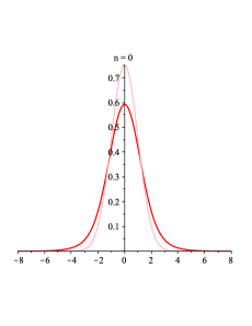
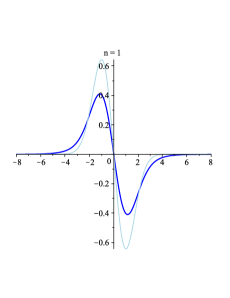
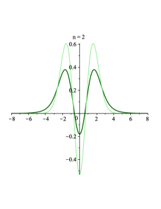
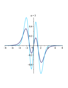
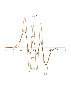
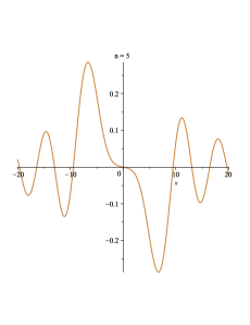
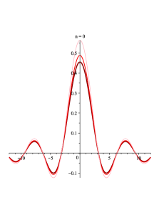
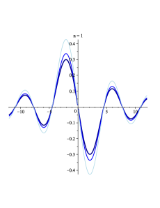
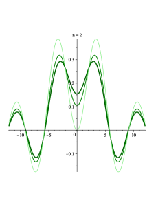
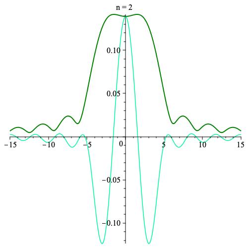
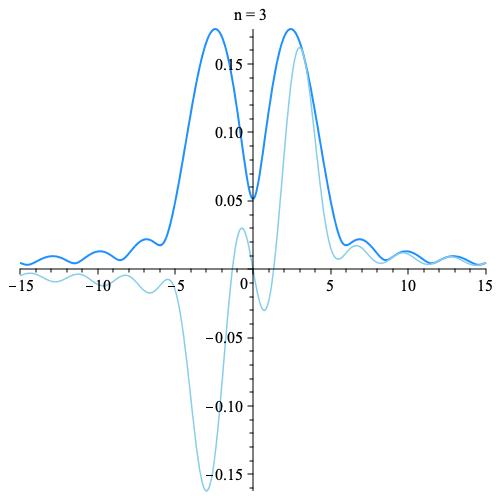
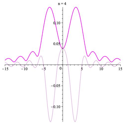
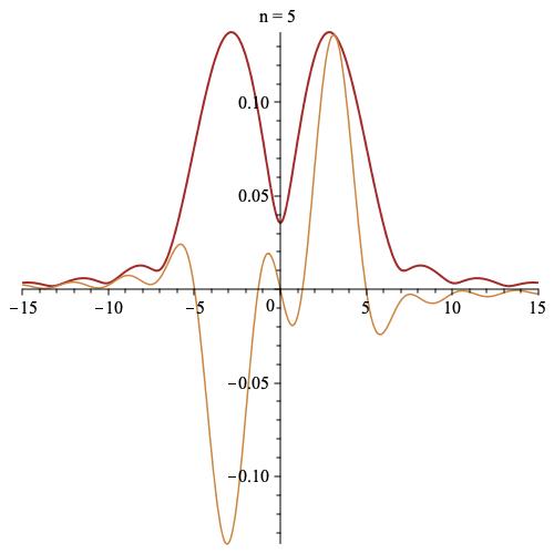
Figure 4.1: The first six functions ฯ†nโŸจ1โŸฉsuperscriptsubscript๐œ‘๐‘›delimited-โŸจโŸฉ1\varphi_{n}^{\langle 1\rangle} defined by (4.1), with corresponding Hermite functions ฯ†nโŸจ0โŸฉโ€‹(x)=(โˆ’1)nโ€‹eโˆ’x2/2โ€‹H~nโ€‹(x)superscriptsubscript๐œ‘๐‘›delimited-โŸจโŸฉ0๐‘ฅsuperscript1๐‘›superscriptesuperscript๐‘ฅ22subscript~H๐‘›๐‘ฅ\varphi_{n}^{\langle 0\rangle}(x)=(-1)^{n}\mathrm{e}^{-x^{2}/2}\tilde{\mathrm{H}}_{n}(x) in darker shade.

In Fig.ย 4.1 we display the functions ฯ†nsubscript๐œ‘๐‘›\varphi_{n}, n=0,โ€ฆ,5๐‘›0โ€ฆ5n=0,\ldots,5, computed by brute-force numerical quadrature. In the background, in fainter colour, we display the familiar Hermite functions which follow from (1.1) and are orthonormal in L2โ€‹(โ„)subscriptL2โ„\mathrm{L}_{2}(\mbox{\Bbb R}) (while, by Theoremย 2, the ฯ†nsubscript๐œ‘๐‘›\varphi_{n}s are orthonormal in H1โ€‹(โ„)superscriptH1โ„\mathrm{H}^{1}(\mbox{\Bbb R})).

4.2 The Hermiteโ€“Sobolev cascade of the second kind

While the polynomials pn[s]superscriptsubscript๐‘๐‘›delimited-[]๐‘ p_{n}^{[s]} from Subsectionย 3.1 are unknown for sโˆˆโ„•๐‘ โ„•s\in\mbox{\Bbb N}, it is possible to generate them, as explained in Sectionย 3 or directly from the moments: in the simplest nontrivial case, s=1๐‘ 1s=1, the moments are

ฮผn=โˆซโˆ’โˆžโˆžฮพnโ€‹(1+ฮพ2)โ€‹eโˆ’ฮพ2โ€‹dฮพ={ฯ€โ€‹(2โ€‹n)!โ€‹(2โ€‹n+3)22โ€‹n+1โ€‹n!,nโ€‹ย even,0,nโ€‹ย odd,subscript๐œ‡๐‘›superscriptsubscriptsuperscript๐œ‰๐‘›1superscript๐œ‰2superscriptesuperscript๐œ‰2differential-d๐œ‰cases๐œ‹2๐‘›2๐‘›3superscript22๐‘›1๐‘›๐‘›ย even,0๐‘›ย odd,\mu_{n}=\int_{-\infty}^{\infty}\xi^{n}(1+\xi^{2})\mathrm{e}^{-\xi^{2}}\,\mathrm{d}\xi=\left\{\begin{array}[]{ll}\displaystyle\frac{\sqrt{\pi}(2n)!(2n+3)}{2^{2n+1}n!},&n\mbox{\ even,}\\[4.0pt] 0,&n\mbox{\ odd,}\end{array}\right.

and the first few pn[1]superscriptsubscript๐‘๐‘›delimited-[]1p_{n}^{[1]}s are

p0[1]โ€‹(ฮพ)superscriptsubscript๐‘0delimited-[]1๐œ‰\displaystyle p_{0}^{[1]}(\xi) โ‰ก\displaystyle\equiv 63โ€‹ฯ€1/4,63superscript๐œ‹14\displaystyle\frac{\sqrt{6}}{3\pi^{1/4}},
p1[1]โ€‹(ฮพ)superscriptsubscript๐‘1delimited-[]1๐œ‰\displaystyle p_{1}^{[1]}(\xi) =\displaystyle= 2โ€‹55โ€‹ฯ€1/4โ€‹ฮพ,255superscript๐œ‹14๐œ‰\displaystyle\frac{2\sqrt{5}}{5\pi^{1/4}}\xi,
p2[1]โ€‹(ฮพ)superscriptsubscript๐‘2delimited-[]1๐œ‰\displaystyle p_{2}^{[1]}(\xi) =\displaystyle= 2โ€‹5719โ€‹ฯ€1/4โ€‹(ฮพ2โˆ’56),25719superscript๐œ‹14superscript๐œ‰256\displaystyle\frac{2\sqrt{57}}{19\pi^{1/4}}\left(\xi^{2}-\frac{5}{6}\right)\!,
p3[1]โ€‹(ฮพ)superscriptsubscript๐‘3delimited-[]1๐œ‰\displaystyle p_{3}^{[1]}(\xi) =\displaystyle= 2โ€‹13039โ€‹ฯ€1/4โ€‹(ฮพ3โˆ’2110โ€‹ฮพ),213039superscript๐œ‹14superscript๐œ‰32110๐œ‰\displaystyle\frac{2\sqrt{130}}{39\pi^{1/4}}\left(\xi^{3}-\frac{21}{10}\xi\right)\!,
p4[1]โ€‹(ฮพ)superscriptsubscript๐‘4delimited-[]1๐œ‰\displaystyle p_{4}^{[1]}(\xi) =\displaystyle= 2โ€‹9861519โ€‹ฯ€1/4โ€‹(ฮพ4โˆ’7519โ€‹ฮพ2+11776),29861519superscript๐œ‹14superscript๐œ‰47519superscript๐œ‰211776\displaystyle\frac{2\sqrt{9861}}{519\pi^{1/4}}\left(\xi^{4}-\frac{75}{19}\xi^{2}+\frac{117}{76}\right)\!,
p5[1]โ€‹(ฮพ)superscriptsubscript๐‘5delimited-[]1๐œ‰\displaystyle p_{5}^{[1]}(\xi) =\displaystyle= 2โ€‹529102035โ€‹ฯ€1/4โ€‹(ฮพ5โˆ’24539โ€‹ฮพ3+33552โ€‹ฮพ)2529102035superscript๐œ‹14superscript๐œ‰524539superscript๐œ‰333552๐œ‰\displaystyle\frac{2\sqrt{52910}}{2035\pi^{1/4}}\left(\xi^{5}-\frac{245}{39}\xi^{3}+\frac{335}{52}\xi\right)

and so on. Likewise, it is possible to compute recurrence coefficients,

b0=56,b1=1915,b2=315190,b3=1730741,b4=3866513494,b5=23692570411formulae-sequencesubscript๐‘056formulae-sequencesubscript๐‘11915formulae-sequencesubscript๐‘2315190formulae-sequencesubscript๐‘31730741formulae-sequencesubscript๐‘43866513494subscript๐‘523692570411b_{0}=\sqrt{\frac{5}{6}},\;b_{1}=\sqrt{\frac{19}{15}},\;b_{2}=\sqrt{\frac{315}{190}},\;b_{3}=\sqrt{\frac{1730}{741}},\;b_{4}=\sqrt{\frac{38665}{13494}},\;b_{5}=\sqrt{\frac{236925}{70411}}

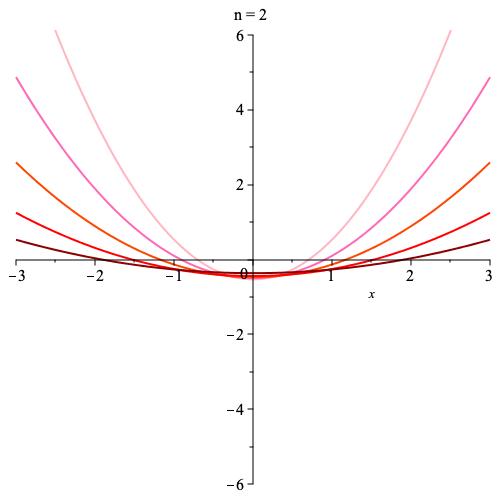
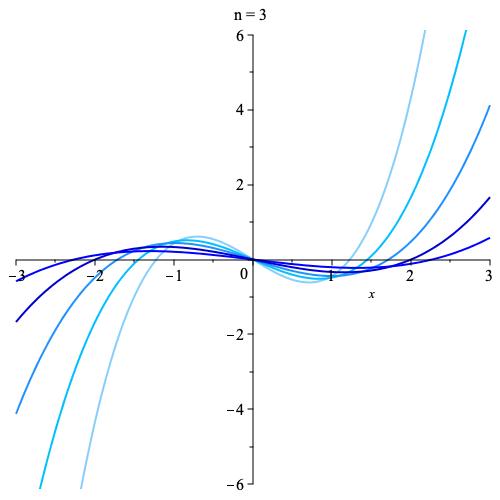
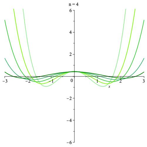
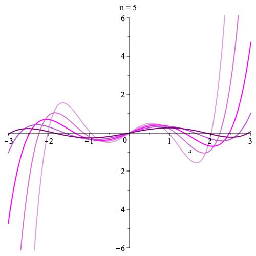
etc.ย but difficult to discern any pattern except for the obvious, bn=๐’ชโ€‹(n1/2)subscript๐‘๐‘›๐’ชsuperscript๐‘›12b_{n}={\cal O}\!\left(n^{1/2}\right), nโ‰ซ1much-greater-than๐‘›1n\gg 1, a consequence of the proof of the Freud conjecture in (?). Likewise, we can compute pn[s]superscriptsubscript๐‘๐‘›delimited-[]๐‘ p_{n}^{[s]} for sโ‰ฅ2๐‘ 2s\geq 2: Fig.ย 4.2 displays pn[s]superscriptsubscript๐‘๐‘›delimited-[]๐‘ p_{n}^{[s]} for n=2,3,4,5๐‘›2345n=2,3,4,5 and s=0,1,2,3,4๐‘ 01234s=0,1,2,3,4.

Refer to caption
Refer to caption
Refer to caption
Refer to caption
Figure 4.2: The polynomials pn[s]superscriptsubscript๐‘๐‘›delimited-[]๐‘ p_{n}^{[s]} for n=2,3,4,5๐‘›2345n=2,3,4,5 and s=0,1,2,4๐‘ 0124s=0,1,2,4 (darker hue corresponds to larger s๐‘ s).

Computing the ฯ†n[1]superscriptsubscript๐œ‘๐‘›delimited-[]1\varphi_{n}^{[1]}s in line with (1.5) is straightforward:

ฯ†0[1]โ€‹(x)superscriptsubscript๐œ‘0delimited-[]1๐‘ฅ\displaystyle\varphi_{0}^{[1]}(x) =\displaystyle= 23โ€‹ฯ€โˆ’1/4โ€‹eโˆ’x2/2,23superscript๐œ‹14superscriptesuperscript๐‘ฅ22\displaystyle\sqrt{\frac{2}{3}}\pi^{-1/4}\mathrm{e}^{-x^{2}/2},
ฯ†1[1]โ€‹(x)superscriptsubscript๐œ‘1delimited-[]1๐‘ฅ\displaystyle\varphi_{1}^{[1]}(x) =\displaystyle= โˆ’45โ€‹ฯ€โˆ’1/4โ€‹xโ€‹eโˆ’x2/2,45superscript๐œ‹14๐‘ฅsuperscriptesuperscript๐‘ฅ22\displaystyle-\sqrt{\frac{4}{5}}\pi^{-1/4}x\mathrm{e}^{-x^{2}/2},
ฯ†2[1]โ€‹(x)superscriptsubscript๐œ‘2delimited-[]1๐‘ฅ\displaystyle\varphi_{2}^{[1]}(x) =\displaystyle= 157โ€‹ฯ€โˆ’1/4โ€‹(6โ€‹x2โˆ’1)โ€‹eโˆ’x2/2,157superscript๐œ‹146superscript๐‘ฅ21superscriptesuperscript๐‘ฅ22\displaystyle\frac{1}{\sqrt{57}}\pi^{-1/4}(6x^{2}-1)\mathrm{e}^{-x^{2}/2},
ฯ†3[1]โ€‹(x)superscriptsubscript๐œ‘3delimited-[]1๐‘ฅ\displaystyle\varphi_{3}^{[1]}(x) =\displaystyle= โˆ’2585โ€‹ฯ€โˆ’1/4โ€‹(10โ€‹x3โˆ’9โ€‹x)โ€‹eโˆ’x2/2,2585superscript๐œ‹1410superscript๐‘ฅ39๐‘ฅsuperscriptesuperscript๐‘ฅ22\displaystyle-\sqrt{\frac{2}{585}}\pi^{-1/4}(10x^{3}-9x)\mathrm{e}^{-x^{2}/2},
ฯ†4[1]โ€‹(x)superscriptsubscript๐œ‘4delimited-[]1๐‘ฅ\displaystyle\varphi_{4}^{[1]}(x) =\displaystyle= 139444โ€‹ฯ€โˆ’1/4โ€‹(76โ€‹x4โˆ’156โ€‹x2+45)โ€‹eโˆ’x2/2,139444superscript๐œ‹1476superscript๐‘ฅ4156superscript๐‘ฅ245superscriptesuperscript๐‘ฅ22\displaystyle\frac{1}{\sqrt{39444}}\pi^{-1/4}(76x^{4}-156x^{2}+45)\mathrm{e}^{-x^{2}/2},
ฯ†5[1]โ€‹(x)superscriptsubscript๐œ‘5delimited-[]1๐‘ฅ\displaystyle\varphi_{5}^{[1]}(x) =\displaystyle= โˆ’1476190โ€‹ฯ€โˆ’1/4โ€‹(156โ€‹x5โˆ’580โ€‹x3+405โ€‹x)โ€‹eโˆ’x2/21476190superscript๐œ‹14156superscript๐‘ฅ5580superscript๐‘ฅ3405๐‘ฅsuperscriptesuperscript๐‘ฅ22\displaystyle-\frac{1}{\sqrt{476190}}\pi^{-1/4}(156x^{5}-580x^{3}+405x)\mathrm{e}^{-x^{2}/2}

and so on.

Refer to captionRefer to caption
Refer to caption
Refer to caption
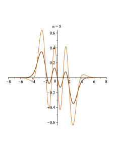
Figure 4.3: The first six functions ฯ†n[1]superscriptsubscript๐œ‘๐‘›delimited-[]1\varphi_{n}^{[1]} with corresponding functions ฯ†n[0]superscriptsubscript๐œ‘๐‘›delimited-[]0\varphi_{n}^{[0]}, which are orthogonal in L2โ€‹(โ„)subscriptL2โ„\mathrm{L}_{2}(\mbox{\Bbb R}), in darker shade.

Fig.ย 4.3 displays the above functions ฯ†n[1]superscriptsubscript๐œ‘๐‘›delimited-[]1\varphi_{n}^{[1]} and, in fainter colour, the functions ฯ†nโŸจ0โŸฉsuperscriptsubscript๐œ‘๐‘›delimited-โŸจโŸฉ0\varphi_{n}^{\langle 0\rangle} based on the same weight wโ€‹(ฮพ)=(1+ฮพ2)โ€‹eโˆ’ฮพ2๐‘ค๐œ‰1superscript๐œ‰2superscriptesuperscript๐œ‰2w(\xi)=(1+\xi^{2})\mathrm{e}^{-\xi^{2}} and defined by (1.1).

Lemma 8

For every nโˆˆโ„ค+๐‘›subscriptโ„คn\in\mbox{\Bbb Z}_{+} we have ฯ†nโ€‹(x)=ฮปnโ€‹(x)โ€‹eโˆ’x2/2subscript๐œ‘๐‘›๐‘ฅsubscript๐œ†๐‘›๐‘ฅsuperscriptesuperscript๐‘ฅ22\varphi_{n}(x)=\lambda_{n}(x)\mathrm{e}^{-x^{2}/2}, where ฮปnsubscript๐œ†๐‘›\lambda_{n} is an n๐‘›nth-degree polynomial.

Proofโ€ƒIt is enough to prove that

ฯƒnโ€‹(x)=in2โ€‹ฯ€โ€‹โˆซโˆ’โˆžโˆžฮพnโ€‹eโˆ’ฮพ2/2+iโ€‹xโ€‹ฮพโ€‹dฮพ,nโˆˆโ„ค+,formulae-sequencesubscript๐œŽ๐‘›๐‘ฅsuperscripti๐‘›2๐œ‹superscriptsubscriptsuperscript๐œ‰๐‘›superscriptesuperscript๐œ‰22i๐‘ฅ๐œ‰differential-d๐œ‰๐‘›subscriptโ„ค\sigma_{n}(x)=\frac{{\mathrm{i}}^{n}}{\sqrt{2\pi}}\int_{-\infty}^{\infty}\xi^{n}\mathrm{e}^{-\xi^{2}/2+{\mathrm{i}}x\xi}\,\mathrm{d}\xi,\qquad n\in\mbox{\Bbb Z}_{+},

is of the asserted form, i.e.ย an n๐‘›nth degree polynomial times eโˆ’x2/2superscriptesuperscript๐‘ฅ22\mathrm{e}^{-x^{2}/2}. This follows readily by induction on n๐‘›n from ฯƒ0โ€‹(x)=eโˆ’x2/2subscript๐œŽ0๐‘ฅsuperscriptesuperscript๐‘ฅ22\sigma_{0}(x)=\mathrm{e}^{-x^{2}/2} and ฯƒnโ€ฒ=ฯƒn+1superscriptsubscript๐œŽ๐‘›โ€ฒsubscript๐œŽ๐‘›1\sigma_{n}^{\prime}=\sigma_{n+1} because, letting ฯƒnโ€‹(x)=ฮฑnโ€‹(x)โ€‹eโˆ’x2/2subscript๐œŽ๐‘›๐‘ฅsubscript๐›ผ๐‘›๐‘ฅsuperscriptesuperscript๐‘ฅ22\sigma_{n}(x)=\alpha_{n}(x)\mathrm{e}^{-x^{2}/2}, we obtain ฮฑn+1โ€‹(x)=ฮฑnโ€ฒโ€‹(x)โˆ’xโ€‹ฮฑnโ€‹(x)subscript๐›ผ๐‘›1๐‘ฅsuperscriptsubscript๐›ผ๐‘›โ€ฒ๐‘ฅ๐‘ฅsubscript๐›ผ๐‘›๐‘ฅ\alpha_{n+1}(x)=\alpha_{n}^{\prime}(x)-x\alpha_{n}(x). ย ย ย ย ย ย  โ–กโ–ก\Box

Alternatively, substituting into (2.1), it is easy to see that

ฮปnโ€ฒโ€‹(x)=โˆ’bnโˆ’1โ€‹ฮปnโˆ’1โ€‹(x)+xโ€‹ฮปnโ€‹(x)+bnโ€‹ฮปn+1โ€‹(x),nโˆˆโ„ค+.formulae-sequencesuperscriptsubscript๐œ†๐‘›โ€ฒ๐‘ฅsubscript๐‘๐‘›1subscript๐œ†๐‘›1๐‘ฅ๐‘ฅsubscript๐œ†๐‘›๐‘ฅsubscript๐‘๐‘›subscript๐œ†๐‘›1๐‘ฅ๐‘›subscriptโ„ค\lambda_{n}^{\prime}(x)=-b_{n-1}\lambda_{n-1}(x)+x\lambda_{n}(x)+b_{n}\lambda_{n+1}(x),\qquad n\in\mbox{\Bbb Z}_{+}.

The proof that ฮปnsubscript๐œ†๐‘›\lambda_{n} is an n๐‘›nth degree polynomial follows at once by induction on this differential recurrence, since bn>0subscript๐‘๐‘›0b_{n}>0, nโˆˆโ„•๐‘›โ„•n\in\mbox{\Bbb N}.

The bad news is that the ฮปnsubscript๐œ†๐‘›\lambda_{n}s are not known and, as is trivial to verify, they do not obey a three-term recurrence relation (hence, by the Favard theorem, cannot be orthogonal with respect to any Borel measure). Having said so, the result is highly interesting. It has been proved in (?) that there exists a unique L2subscriptL2\mathrm{L}_{2}-orthonormal system on the real line which obeys (1.2) and where each function is a polynomial multiple of the same L2subscriptL2\mathrm{L}_{2} function, specifically Hermite functions (or ฯ†n[0]=ฯ†nโŸจ0โŸฉsuperscriptsubscript๐œ‘๐‘›delimited-[]0superscriptsubscript๐œ‘๐‘›delimited-โŸจโŸฉ0\varphi_{n}^{[0]}=\varphi_{n}^{\langle 0\rangle} in present notation). The functions {ฯ†n[1]}nโˆˆโ„ค+subscriptsuperscriptsubscript๐œ‘๐‘›delimited-[]1๐‘›subscriptโ„ค\{\varphi_{n}^{[1]}\}_{n\in\mbox{\sBbb Z}_{+}}, though, are H1superscriptH1\mathrm{H}^{1}-orthonormal, they obey (1.2) and ฯ†n[1]โ€‹(x)=eโˆ’x2/2โ€‹ฮปnโ€‹(x)superscriptsubscript๐œ‘๐‘›delimited-[]1๐‘ฅsuperscriptesuperscript๐‘ฅ22subscript๐œ†๐‘›๐‘ฅ\varphi_{n}^{[1]}(x)=\mathrm{e}^{-x^{2}/2}\lambda_{n}(x).

Lemma 9

The only Hvโ€‹(โ„)subscriptH๐‘ฃโ„\mathrm{H}_{v}(\mbox{\Bbb R})-orthonormal systems (see equation (2.5)) with a tridiagonal differentiation matrix which are of the form ฯ†nโ€‹(x)=Gโ€‹(x)โ€‹ฮปnโ€‹(x)subscript๐œ‘๐‘›๐‘ฅ๐บ๐‘ฅsubscript๐œ†๐‘›๐‘ฅ\varphi_{n}(x)=G(x)\lambda_{n}(x), nโˆˆโ„ค+๐‘›subscriptโ„คn\in\mbox{\Bbb Z}_{+}, for some function GโˆˆL2โ€‹(โ„)๐บsubscriptL2โ„G\in\mathrm{L}_{2}(\mbox{\Bbb R}), G>0๐บ0G>0 (and Gโ€‹(0)=1๐บ01G(0)=1 without loss of generality), where each ฮปnsubscript๐œ†๐‘›\lambda_{n} is a polynomial of degree n๐‘›n, correspond to

Gโ€‹(x)=expโก(โˆ’ฮณโ€‹x2+ฮดโ€‹x)๐บ๐‘ฅ๐›พsuperscript๐‘ฅ2๐›ฟ๐‘ฅG(x)=\exp\left(-\gamma x^{2}+\delta x\right) (4.2)

for some constants ฮณ>0๐›พ0\gamma>0 and ฮดโˆˆโ„๐›ฟโ„\delta\in\mbox{\Bbb R}. The corresponding weight of orthonormality for P๐‘ƒP in Theorem 1 is

wโ€‹(ฮพ)โˆvโ€‹(ฮพ)โ€‹eโˆ’ฮพ2/(2โ€‹ฮณ).proportional-to๐‘ค๐œ‰๐‘ฃ๐œ‰superscriptesuperscript๐œ‰22๐›พw(\xi)\propto v(\xi)\mathrm{e}^{-\xi^{2}/(2\gamma)}. (4.3)

Proofโ€ƒWe substitute ฯ†nโ€‹(x)=Gโ€‹(x)โ€‹ฮปnโ€‹(x)subscript๐œ‘๐‘›๐‘ฅ๐บ๐‘ฅsubscript๐œ†๐‘›๐‘ฅ\varphi_{n}(x)=G(x)\lambda_{n}(x) into (2.1), bearing in mind that G>0๐บ0G>0, to obtain,

ฮปnโ€ฒโ€‹(x)=โˆ’bnโˆ’1โ€‹ฮปnโˆ’1โ€‹(x)+(iโ€‹cnโˆ’Gโ€ฒโ€‹(x)Gโ€‹(x))โ€‹ฮปnโ€‹(x)+bnโ€‹ฮปn+1โ€‹(x),nโˆˆโ„ค+.formulae-sequencesuperscriptsubscript๐œ†๐‘›โ€ฒ๐‘ฅsubscript๐‘๐‘›1subscript๐œ†๐‘›1๐‘ฅisubscript๐‘๐‘›superscript๐บโ€ฒ๐‘ฅ๐บ๐‘ฅsubscript๐œ†๐‘›๐‘ฅsubscript๐‘๐‘›subscript๐œ†๐‘›1๐‘ฅ๐‘›subscriptโ„ค\lambda_{n}^{\prime}(x)=-b_{n-1}\lambda_{n-1}(x)+\left({\mathrm{i}}c_{n}-\frac{G^{\prime}(x)}{G(x)}\right)\lambda_{n}(x)+b_{n}\lambda_{n+1}(x),\qquad n\in\mbox{\Bbb Z}_{+}.

Since degโกฮปm=mdegreesubscript๐œ†๐‘š๐‘š\deg\lambda_{m}=m by assumption, we deduce, comparing degrees, that Gโ€ฒ/Gsuperscript๐บโ€ฒ๐บG^{\prime}/G is a linear polynomial, and hence that Gโ€‹(x)๐บ๐‘ฅG(x) is the exponential of a quadratic polynomial. We can set the constant term in this quadratic to zero since Gโ€‹(0)=1๐บ01G(0)=1 without loss of generality, so we obtain equation (4.2).

Inverting the representation in Theorem 1, we have

pnโ€‹(ฮพ)โ€‹gโ€‹(ฮพ)=(โˆ’i)n2โ€‹ฯ€โ€‹โˆซโˆ’โˆžโˆžฯ†nโ€‹(x)โ€‹eโˆ’iโ€‹xโ€‹ฮพโ€‹dx=(โˆ’i)n2โ€‹ฯ€โ€‹โˆซโˆ’โˆžโˆžฮปnโ€‹(x)โ€‹eโˆ’ฮณโ€‹x2โ€‹ฮพ+ฮดโ€‹xโˆ’iโ€‹xโ€‹ฮพโ€‹dx.subscript๐‘๐‘›๐œ‰๐‘”๐œ‰superscripti๐‘›2๐œ‹superscriptsubscriptsubscript๐œ‘๐‘›๐‘ฅsuperscriptei๐‘ฅ๐œ‰differential-d๐‘ฅsuperscripti๐‘›2๐œ‹superscriptsubscriptsubscript๐œ†๐‘›๐‘ฅsuperscripte๐›พsuperscript๐‘ฅ2๐œ‰๐›ฟ๐‘ฅi๐‘ฅ๐œ‰differential-d๐‘ฅp_{n}(\xi)g(\xi)=\frac{(-{\mathrm{i}})^{n}}{\sqrt{2\pi}}\int_{-\infty}^{\infty}\varphi_{n}(x)\mathrm{e}^{-{\mathrm{i}}x\xi}\,\mathrm{d}x=\frac{(-{\mathrm{i}})^{n}}{\sqrt{2\pi}}\int_{-\infty}^{\infty}\lambda_{n}(x)\mathrm{e}^{-\gamma x^{2}\xi+\delta x-{\mathrm{i}}x\xi}\,\mathrm{d}x.

The case n=0๐‘›0n=0 tells us that

gโ€‹(ฮพ)โˆexpโก(โˆ’(ฮพโˆ’iโ€‹ฮด)2/(4โ€‹ฮณ)).proportional-to๐‘”๐œ‰superscript๐œ‰i๐›ฟ24๐›พg(\xi)\propto\exp(-(\xi-{\mathrm{i}}\delta)^{2}/(4\gamma)). (4.4)

Theoremย 2 tells us that for Hvโ€‹(โ„)subscriptH๐‘ฃโ„\mathrm{H}_{v}(\mbox{\Bbb R}) orthonormality we require

wโ€‹(ฮพ)=vโ€‹(ฮพ)โ€‹|gโ€‹(ฮพ)|2,๐‘ค๐œ‰๐‘ฃ๐œ‰superscript๐‘”๐œ‰2w(\xi)=v(\xi)|g(\xi)|^{2}, (4.5)

which completes the proof of necessity of the forms of G๐บG and w๐‘คw.

Now we prove sufficiency. Let wโ€‹(ฮพ)=C2โ€‹vโ€‹(ฮพ)โ€‹eโˆ’ฮพ2/2โ€‹ฮณ๐‘ค๐œ‰superscript๐ถ2๐‘ฃ๐œ‰superscriptesuperscript๐œ‰22๐›พw(\xi)=C^{2}v(\xi)\mathrm{e}^{-\xi^{2}/2\gamma} where C๐ถC ensures w๐‘คw has unit integral, gโ€‹(ฮพ)=Cโ€‹eโˆ’(ฮพโˆ’iโ€‹ฮด)2/(4โ€‹ฮณ)๐‘”๐œ‰๐ถsuperscriptesuperscript๐œ‰i๐›ฟ24๐›พg(\xi)=C\mathrm{e}^{-(\xi-{\mathrm{i}}\delta)^{2}/(4\gamma)}, and define ฮฆฮฆ\Phi as in Theorem 1. By Theorem 4, ฮฆฮฆ\Phi is an Hvโ€‹(โ„)subscriptH๐‘ฃโ„\mathrm{H}_{v}(\mbox{\Bbb R})-orthonormal system, so all that remains to prove is that ฯ†nโ€‹(x)=Gโ€‹(x)โ€‹ฮปnโ€‹(x)subscript๐œ‘๐‘›๐‘ฅ๐บ๐‘ฅsubscript๐œ†๐‘›๐‘ฅ\varphi_{n}(x)=G(x)\lambda_{n}(x) where ฮปnsubscript๐œ†๐‘›\lambda_{n} is a polynomial of degree n๐‘›n. It is sufficient to show that ฯnโ€‹(x)=โˆซโˆ’โˆžโˆžฮพnโ€‹gโ€‹(ฮพ)โ€‹eiโ€‹xโ€‹ฮพโ€‹dฮพsubscript๐œŒ๐‘›๐‘ฅsuperscriptsubscriptsuperscript๐œ‰๐‘›๐‘”๐œ‰superscriptei๐‘ฅ๐œ‰differential-d๐œ‰\rho_{n}(x)=\int_{-\infty}^{\infty}\xi^{n}g(\xi)\mathrm{e}^{{\mathrm{i}}x\xi}\,\,\mathrm{d}\xi is Gโ€‹(x)๐บ๐‘ฅG(x) times a polynomial of degree n๐‘›n, which can be readily shown by induction starting from ฯ0โ€‹(x)โˆGโ€‹(x)proportional-tosubscript๐œŒ0๐‘ฅ๐บ๐‘ฅ\rho_{0}(x)\propto G(x) and leveraging ฯn+1โ€‹(x)=โˆ’iโ€‹ฯnโ€ฒโ€‹(x)subscript๐œŒ๐‘›1๐‘ฅisuperscriptsubscript๐œŒ๐‘›โ€ฒ๐‘ฅ\rho_{n+1}(x)=-{\mathrm{i}}\rho_{n}^{\prime}(x). ย ย ย ย ย ย  โ–กโ–ก\Box

4.3 An Hโˆžโ€‹(โ„)superscriptHโ„\mathrm{H}^{\infty}(\mbox{\Bbb R}) system based on the Hermite weight

Let ฯƒโˆˆ(0,1)๐œŽ01\sigma\in(0,1), wโ€‹(ฮพ)=eโˆ’ฮพ2๐‘ค๐œ‰superscriptesuperscript๐œ‰2w(\xi)=\mathrm{e}^{-\xi^{2}} (i.e.ย the standard Hermite weight) and vโ€‹(ฮพ)=eฯƒโ€‹ฮพ2๐‘ฃ๐œ‰superscripte๐œŽsuperscript๐œ‰2v(\xi)=\mathrm{e}^{\sigma\xi^{2}}, ฮพโˆˆโ„๐œ‰โ„\xi\in\mbox{\Bbb R}. Therefore, by Theoremย 3, the functions ฯ†nsubscript๐œ‘๐‘›\varphi_{n}, as defined by (2.3), are orthogonal with respect to the infinite Sobolev inner product

โŸจf,gโŸฉv=โˆ‘โ„“=0โˆžฯƒโ„“โ„“!โ€‹โˆซโˆ’โˆžโˆžf(โ„“)โ€‹(x)โ€‹g(โ„“)โ€‹(x)โ€‹dx.subscript๐‘“๐‘”๐‘ฃsuperscriptsubscriptโ„“0superscript๐œŽโ„“โ„“superscriptsubscriptsuperscript๐‘“โ„“๐‘ฅsuperscript๐‘”โ„“๐‘ฅdifferential-d๐‘ฅ\langle f,g\rangle_{v}=\sum_{\ell=0}^{\infty}\frac{\sigma^{\ell}}{\ell!}\int_{-\infty}^{\infty}f^{(\ell)}(x)g^{(\ell)}(x)\,\mathrm{d}x. (4.6)

In this case pnsubscript๐‘๐‘›p_{n}s are scaled Hermite polynomials and ฯ†nsubscript๐œ‘๐‘›\varphi_{n}s can be computed explicitly.

Theorem 10

The Hermite weight wโ€‹(ฮพ)=eโˆ’ฮพ2๐‘ค๐œ‰superscriptesuperscript๐œ‰2w(\xi)=\mathrm{e}^{-\xi^{2}}, xโˆˆโ„๐‘ฅโ„x\in\mbox{\Bbb R}, generates the Hโˆžโ€‹(โ„)superscriptHโ„\mathrm{H}^{\infty}(\mbox{\Bbb R}) system

ฯ†n[โˆž]โ€‹(x)=11+ฯƒโ€‹(1โˆ’ฯƒ1+ฯƒ)n/2โ€‹ฯ†n[0]โ€‹(x1โˆ’ฯƒ2)โ€‹expโก(ฯƒโ€‹x22โ€‹(1โˆ’ฯƒ2)),nโˆˆโ„ค+,formulae-sequencesuperscriptsubscript๐œ‘๐‘›delimited-[]๐‘ฅ11๐œŽsuperscript1๐œŽ1๐œŽ๐‘›2superscriptsubscript๐œ‘๐‘›delimited-[]0๐‘ฅ1superscript๐œŽ2๐œŽsuperscript๐‘ฅ221superscript๐œŽ2๐‘›subscriptโ„ค\varphi_{n}^{[\infty]}(x)=\frac{1}{\sqrt{1+\sigma}}\left(\frac{1-\sigma}{1+\sigma}\right)^{\!n/2}\varphi_{n}^{[0]}\!\left(\frac{x}{\sqrt{1-\sigma^{2}}}\right)\!\exp\!\left(\frac{\sigma x^{2}}{2(1-\sigma^{2})}\right)\!,\qquad n\in\mbox{\Bbb Z}_{+}, (4.7)

where ฯ†n[0]superscriptsubscript๐œ‘๐‘›delimited-[]0\varphi_{n}^{[0]} is the standard n๐‘›nth Hermite function.

Proofโ€ƒLet

ฯ†~nโ€‹(x)=in2โ€‹ฯ€โ€‹โˆซโˆ’โˆžโˆžHnโ€‹(ฮพ)โ€‹eโˆ’12โ€‹(1+ฯƒ)โ€‹ฮพ2+iโ€‹xโ€‹ฮพโ€‹dฮพ,nโˆˆโ„ค+,formulae-sequencesubscript~๐œ‘๐‘›๐‘ฅsuperscripti๐‘›2๐œ‹superscriptsubscriptsubscriptH๐‘›๐œ‰superscripte121๐œŽsuperscript๐œ‰2i๐‘ฅ๐œ‰differential-d๐œ‰๐‘›subscriptโ„ค\tilde{\varphi}_{n}(x)=\frac{{\mathrm{i}}^{n}}{\sqrt{2\pi}}\int_{-\infty}^{\infty}\mathrm{H}_{n}(\xi)\mathrm{e}^{-\frac{1}{2}(1+\sigma)\xi^{2}+{\mathrm{i}}x\xi}\,\mathrm{d}\xi,\qquad n\in\mbox{\Bbb Z}_{+},

whereby, orthonormalising Hermite polynomials, (2.3) yields ฯ†nโ€‹(x)=ฯ†~nโ€‹(x)/2nโ€‹n!โ€‹ฯ€subscript๐œ‘๐‘›๐‘ฅsubscript~๐œ‘๐‘›๐‘ฅsuperscript2๐‘›๐‘›๐œ‹\varphi_{n}(x)=\tilde{\varphi}_{n}(x)/\sqrt{2^{n}n!\sqrt{\pi}}. Using the standard generating function for Hermite polynomials,

โˆ‘n=0โˆžฯ†~nโ€‹(x)n!โ€‹tnsuperscriptsubscript๐‘›0subscript~๐œ‘๐‘›๐‘ฅ๐‘›superscript๐‘ก๐‘›\displaystyle\sum_{n=0}^{\infty}\frac{\tilde{\varphi}_{n}(x)}{n!}t^{n} =\displaystyle= 12โ€‹ฯ€โ€‹โˆซโˆ’โˆžโˆž[โˆ‘n=0โˆžHnโ€‹(ฮพ)n!โ€‹(iโ€‹t)n]โ€‹expโก(โˆ’1+ฯƒ2โ€‹ฮพ2+iโ€‹xโ€‹ฮพ)โ€‹dฮพ12๐œ‹superscriptsubscriptdelimited-[]superscriptsubscript๐‘›0subscriptH๐‘›๐œ‰๐‘›superscripti๐‘ก๐‘›1๐œŽ2superscript๐œ‰2i๐‘ฅ๐œ‰differential-d๐œ‰\displaystyle\frac{1}{\sqrt{2\pi}}\int_{-\infty}^{\infty}\left[\sum_{n=0}^{\infty}\frac{\mathrm{H}_{n}(\xi)}{n!}({\mathrm{i}}t)^{n}\right]\!\exp\!\left(-\frac{1+\sigma}{2}\xi^{2}+{\mathrm{i}}x\xi\right)\!\,\mathrm{d}\xi
=\displaystyle= 12โ€‹ฯ€โ€‹โˆซโˆ’โˆžโˆžexpโก(2โ€‹iโ€‹ฮพโ€‹t+t2โˆ’1+ฯƒ2โ€‹ฮพ2+iโ€‹xโ€‹ฮพ)โ€‹dฮพ12๐œ‹superscriptsubscript2i๐œ‰๐‘กsuperscript๐‘ก21๐œŽ2superscript๐œ‰2i๐‘ฅ๐œ‰differential-d๐œ‰\displaystyle\frac{1}{\sqrt{2\pi}}\int_{-\infty}^{\infty}\exp\!\left(2{\mathrm{i}}\xi t+t^{2}-\frac{1+\sigma}{2}\xi^{2}+{\mathrm{i}}x\xi\right)\!\,\mathrm{d}\xi
=\displaystyle= 11+ฯƒโ€‹expโก(โˆ’x22โ€‹(1+ฯƒ))โ€‹expโก(โˆ’2โ€‹xโ€‹t1+ฯƒโˆ’1โˆ’ฯƒ1+ฯƒโ€‹t2)11๐œŽsuperscript๐‘ฅ221๐œŽ2๐‘ฅ๐‘ก1๐œŽ1๐œŽ1๐œŽsuperscript๐‘ก2\displaystyle\frac{1}{\sqrt{1+\sigma}}\exp\!\left(-\frac{x^{2}}{2(1+\sigma)}\right)\!\exp\!\left(-\frac{2xt}{1+\sigma}-\frac{1-\sigma}{1+\sigma}t^{2}\right)
=\displaystyle= 11+ฯƒโ€‹expโก(โˆ’x22โ€‹(1+ฯƒ))โ€‹expโก(โˆ’2โ€‹x1โˆ’ฯƒ2โ€‹(1โˆ’ฯƒ1+ฯƒโ€‹t)โˆ’(1โˆ’ฯƒ1+ฯƒโ€‹t)2)11๐œŽsuperscript๐‘ฅ221๐œŽ2๐‘ฅ1superscript๐œŽ21๐œŽ1๐œŽ๐‘กsuperscript1๐œŽ1๐œŽ๐‘ก2\displaystyle\frac{1}{\sqrt{1+\sigma}}\exp\!\left(-\frac{x^{2}}{2(1+\sigma)}\right)\!\exp\!\left(-\frac{2x}{\sqrt{1-\sigma^{2}}}\left(\sqrt{\frac{1\!-\!\sigma}{1\!+\!\sigma}}t\right)-\left(\sqrt{\frac{1\!-\!\sigma}{1\!+\!\sigma}}t\right)^{\!2}\right)

and, using the same generating function in the opposite direction,

โˆ‘n=0โˆžฯ†~nโ€‹(x)n!โ€‹tnsuperscriptsubscript๐‘›0subscript~๐œ‘๐‘›๐‘ฅ๐‘›superscript๐‘ก๐‘›\displaystyle\sum_{n=0}^{\infty}\frac{\tilde{\varphi}_{n}(x)}{n!}t^{n} =\displaystyle= 11+ฯƒโ€‹expโก(โˆ’x22โ€‹(1+ฯƒ))โ€‹โˆ‘n=0โˆž1n!โ€‹Hnโ€‹(โˆ’x1โˆ’ฯƒ2)โ€‹(1โˆ’ฯƒ1+ฯƒโ€‹t)n.11๐œŽsuperscript๐‘ฅ221๐œŽsuperscriptsubscript๐‘›01๐‘›subscriptH๐‘›๐‘ฅ1superscript๐œŽ2superscript1๐œŽ1๐œŽ๐‘ก๐‘›\displaystyle\frac{1}{\sqrt{1+\sigma}}\exp\!\left(-\frac{x^{2}}{2(1+\sigma)}\right)\!\sum_{n=0}^{\infty}\frac{1}{n!}\mathrm{H}_{n}\!\left(-\frac{x}{\sqrt{1-\sigma^{2}}}\right)\!\left(\sqrt{\frac{1-\sigma}{1+\sigma}}t\right)^{\!n}.

Therefore

ฯ†~nโ€‹(x)=(โˆ’1)n1+ฯƒโ€‹(1โˆ’ฯƒ1+ฯƒ)n/2โ€‹Hnโ€‹(x1โˆ’ฯƒ2)โ€‹expโก(โˆ’x22โ€‹(1+ฯƒ)).subscript~๐œ‘๐‘›๐‘ฅsuperscript1๐‘›1๐œŽsuperscript1๐œŽ1๐œŽ๐‘›2subscriptH๐‘›๐‘ฅ1superscript๐œŽ2superscript๐‘ฅ221๐œŽ\tilde{\varphi}_{n}(x)=\frac{(-1)^{n}}{\sqrt{1+\sigma}}\left(\frac{1-\sigma}{1+\sigma}\right)^{\!n/2}\mathrm{H}_{n}\!\left(\frac{x}{\sqrt{1-\sigma^{2}}}\right)\!\exp\!\left(-\frac{x^{2}}{2(1+\sigma)}\right)\!.

Normalising,

ฯ†n[โˆž]โ€‹(x)superscriptsubscript๐œ‘๐‘›delimited-[]๐‘ฅ\displaystyle\varphi_{n}^{[\infty]}(x) =\displaystyle= (โˆ’1)n(1+ฯƒ)โ€‹2nโ€‹n!โ€‹ฯ€โ€‹(1โˆ’ฯƒ1+ฯƒ)n/2โ€‹Hnโ€‹(x1โˆ’ฯƒ2)โ€‹expโก(โˆ’x22โ€‹(1+ฯƒ)),superscript1๐‘›1๐œŽsuperscript2๐‘›๐‘›๐œ‹superscript1๐œŽ1๐œŽ๐‘›2subscriptH๐‘›๐‘ฅ1superscript๐œŽ2superscript๐‘ฅ221๐œŽ\displaystyle\frac{(-1)^{n}}{\sqrt{(1+\sigma)2^{n}n!\sqrt{\pi}}}\left(\frac{1-\sigma}{1+\sigma}\right)^{\!n/2}\mathrm{H}_{n}\!\left(\frac{x}{\sqrt{1-\sigma^{2}}}\right)\!\exp\!\left(-\frac{x^{2}}{2(1+\sigma)}\right)\!,
=\displaystyle= 11+ฯƒโ€‹(1โˆ’ฯƒ1+ฯƒ)n/2โ€‹ฯ†n[0]โ€‹(x1โˆ’ฯƒ2)โ€‹expโก(ฯƒโ€‹x22โ€‹(1โˆ’ฯƒ2)),nโˆˆโ„ค+,11๐œŽsuperscript1๐œŽ1๐œŽ๐‘›2superscriptsubscript๐œ‘๐‘›delimited-[]0๐‘ฅ1superscript๐œŽ2๐œŽsuperscript๐‘ฅ221superscript๐œŽ2๐‘›subscriptโ„ค\displaystyle\frac{1}{\sqrt{1+\sigma}}\left(\frac{1-\sigma}{1+\sigma}\right)^{\!n/2}\varphi_{n}^{[0]}\!\left(\frac{x}{\sqrt{1-\sigma^{2}}}\right)\!\exp\!\left(\frac{\sigma x^{2}}{2(1-\sigma^{2})}\right)\!,\qquad n\in\mbox{\Bbb Z}_{+},

and (4.7) is true. ย ย ย ย ย ย  โ–กโ–ก\Box

Refer to caption
Refer to caption
Refer to caption
Refer to caption
Refer to caption
Refer to caption
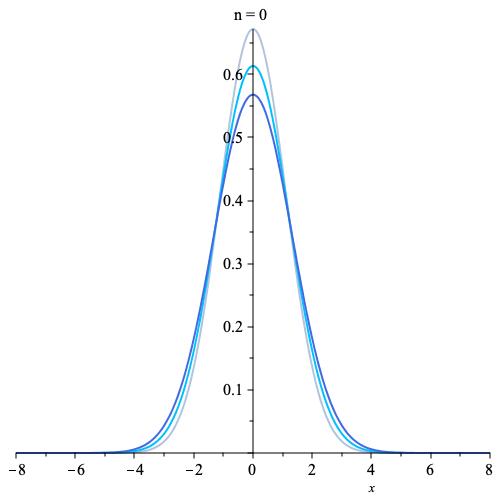
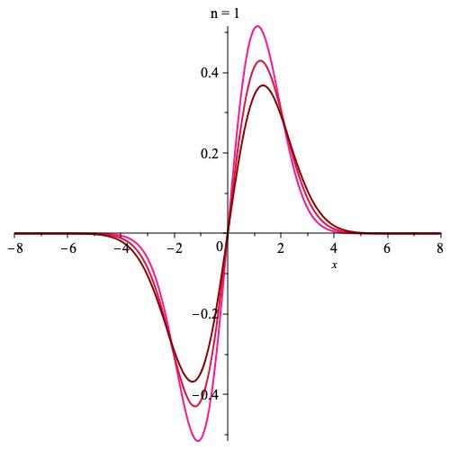
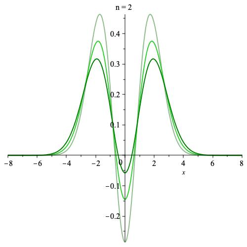
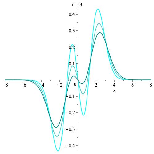
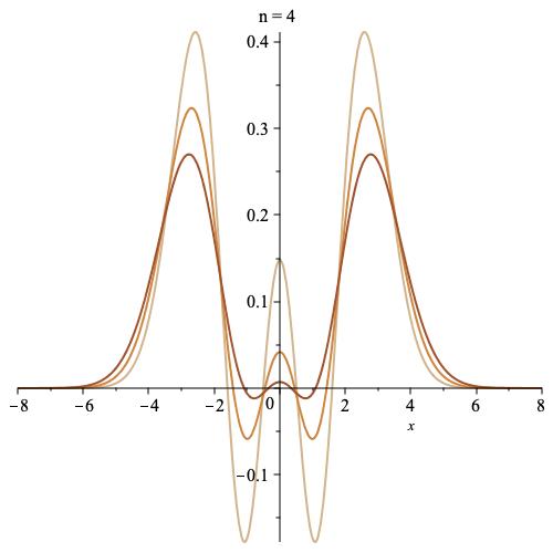
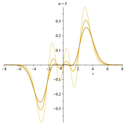
Figure 4.4: The first six HโˆžsuperscriptH\mathrm{H}^{\infty} Hermite-type functions ฯ†n[โˆž]superscriptsubscript๐œ‘๐‘›delimited-[]\varphi_{n}^{[\infty]} for ฯƒ=14,12,34๐œŽ141234\sigma=\frac{1}{4},\frac{1}{2},\frac{3}{4} in progressively darker hues.

Fig.ย 4.4 displays the functions ฯ†n[โˆž]superscriptsubscript๐œ‘๐‘›delimited-[]\varphi_{n}^{[\infty]}, n=0,โ€ฆ,5๐‘›0โ€ฆ5n=0,\ldots,5, for three different values of ฯƒโˆˆ(0,1)๐œŽ01\sigma\in(0,1). The zeros of ฯ†nsubscript๐œ‘๐‘›\varphi_{n} are scaled zeros of a Hermite polynomial and, the scaling being monotone, the zeros are โ€˜squeezedโ€™ in a uniform manner for increasing ฯƒ๐œŽ\sigma, as evident in the figure.

5 Bilateral Laguerre-type weights

Deferring the standard Laguerre weight (which is not symmetric) to Sectionย 7, we let wโ€‹(ฮพ)=(1+ฮพ2)โ€‹eโˆ’|ฮพ|๐‘ค๐œ‰1superscript๐œ‰2superscripte๐œ‰w(\xi)=(1+\xi^{2})\mathrm{e}^{-|\xi|}, ฮพโˆˆโ„๐œ‰โ„\xi\in\mbox{\Bbb R}. Note that the underlying orthogonal polynomials are unknown explicitly, yet can be computed. The ฯ†n[1]superscriptsubscript๐œ‘๐‘›delimited-[]1\varphi_{n}^{[1]}s are

ฯ†0[1]โ€‹(x)superscriptsubscript๐œ‘0delimited-[]1๐‘ฅ\displaystyle\varphi_{0}^{[1]}(x) =\displaystyle= 23โ€‹ฯ€โ€‹11+4โ€‹x2,23๐œ‹114superscript๐‘ฅ2\displaystyle\frac{2}{\sqrt{3}\sqrt{\pi}}\frac{1}{1+4x^{2}},
ฯ†1[1]โ€‹(x)superscriptsubscript๐œ‘1delimited-[]1๐‘ฅ\displaystyle\varphi_{1}^{[1]}(x) =\displaystyle= 1626โ€‹ฯ€โ€‹x(1+4โ€‹x2)2,1626๐œ‹๐‘ฅsuperscript14superscript๐‘ฅ22\displaystyle\frac{16}{\sqrt{26}\sqrt{\pi}}\frac{x}{(1+4x^{2})^{2}},
ฯ†2[1]โ€‹(x)superscriptsubscript๐œ‘2delimited-[]1๐‘ฅ\displaystyle\varphi_{2}^{[1]}(x) =\displaystyle= 21167โ€‹ฯ€โ€‹1+248โ€‹x2+208โ€‹x4(1+4โ€‹x2)3,21167๐œ‹1248superscript๐‘ฅ2208superscript๐‘ฅ4superscript14superscript๐‘ฅ23\displaystyle\frac{2}{\sqrt{1167}\sqrt{\pi}}\frac{1+248x^{2}+208x^{4}}{(1+4x^{2})^{3}},
ฯ†3[1]โ€‹(x)superscriptsubscript๐œ‘3delimited-[]1๐‘ฅ\displaystyle\varphi_{3}^{[1]}(x) =\displaystyle= 1623179โ€‹ฯ€โ€‹โˆ’21โ€‹x+456โ€‹x3+496โ€‹x5(1+4โ€‹x2)4,1623179๐œ‹21๐‘ฅ456superscript๐‘ฅ3496superscript๐‘ฅ5superscript14superscript๐‘ฅ24\displaystyle\frac{16}{\sqrt{23179}\sqrt{\pi}}\frac{-21x+456x^{3}+496x^{5}}{(1+4x^{2})^{4}},
ฯ†4[1]โ€‹(x)superscriptsubscript๐œ‘4delimited-[]1๐‘ฅ\displaystyle\varphi_{4}^{[1]}(x) =\displaystyle= 2309347971โ€‹ฯ€โ€‹2925โˆ’128784โ€‹x2+1703264โ€‹x4+3029760โ€‹x6+1369344โ€‹x8(1+4โ€‹x2)5,2309347971๐œ‹2925128784superscript๐‘ฅ21703264superscript๐‘ฅ43029760superscript๐‘ฅ61369344superscript๐‘ฅ8superscript14superscript๐‘ฅ25\displaystyle\frac{2}{\sqrt{309347971}\sqrt{\pi}}\frac{2925-128784x^{2}+1703264x^{4}+3029760x^{6}+1369344x^{8}}{(1+4x^{2})^{5}},
ฯ†5[1]โ€‹(x)superscriptsubscript๐œ‘5delimited-[]1๐‘ฅ\displaystyle\varphi_{5}^{[1]}(x) =\displaystyle= 1622678864934โ€‹ฯ€โ€‹25749โ€‹xโˆ’1017424โ€‹x3+5715040โ€‹x5+13510400โ€‹x7+7744768โ€‹x9(1+4โ€‹x2)6.1622678864934๐œ‹25749๐‘ฅ1017424superscript๐‘ฅ35715040superscript๐‘ฅ513510400superscript๐‘ฅ77744768superscript๐‘ฅ9superscript14superscript๐‘ฅ26\displaystyle\frac{16}{\sqrt{22678864934}\sqrt{\pi}}\frac{25749x\!-\!1017424x^{3}\!+\!5715040x^{5}\!+\!13510400x^{7}\!+\!7744768x^{9}}{(1+4x^{2})^{6}}.

The general formula is a polynomial of degree 2โ€‹nโˆ’[1โˆ’(โˆ’1)n]/22๐‘›delimited-[]1superscript1๐‘›22n-[1-(-1)^{n}]/2 in x๐‘ฅx (of the same parity as n๐‘›n), divided by (1+4โ€‹x2)n+1superscript14superscript๐‘ฅ2๐‘›1(1+4x^{2})^{n+1}. This can be easily verified because by (2.3) and gโ€‹(ฮพ)=eโˆ’|ฮพ|/2๐‘”๐œ‰superscripte๐œ‰2g(\xi)=\mathrm{e}^{-|\xi|/2} each ฯ†n[1]superscriptsubscript๐œ‘๐‘›delimited-[]1\varphi_{n}^{[1]} is a linear combination of ฮปn,ฮปnโˆ’2,โ€ฆsubscript๐œ†๐‘›subscript๐œ†๐‘›2โ€ฆ\lambda_{n},\lambda_{n-2},\ldots, where

ฮปnโ€‹(x)=in2โ€‹ฯ€โ€‹โˆซโˆ’โˆžโˆžฮพnโ€‹eโˆ’|ฮพ|2+iโ€‹xโ€‹ฮพโ€‹dฮพ,nโˆˆโ„ค+formulae-sequencesubscript๐œ†๐‘›๐‘ฅsuperscripti๐‘›2๐œ‹superscriptsubscriptsuperscript๐œ‰๐‘›superscriptesuperscript๐œ‰2i๐‘ฅ๐œ‰differential-d๐œ‰๐‘›subscriptโ„ค\lambda_{n}(x)=\frac{{\mathrm{i}}^{n}}{\sqrt{2\pi}}\int_{-\infty}^{\infty}\xi^{n}\mathrm{e}^{-|\xi|^{2}+{\mathrm{i}}x\xi}\,\mathrm{d}\xi,\qquad n\in\mbox{\Bbb Z}_{+}

and ฮปnโ€ฒโ€‹(x)=ฮปn+1โ€‹(x)superscriptsubscript๐œ†๐‘›โ€ฒ๐‘ฅsubscript๐œ†๐‘›1๐‘ฅ\lambda_{n}^{\prime}(x)=\lambda_{n+1}(x) implies that

ฮปnโ€‹(x)=ฮป0(n)โ€‹(x)=2โ€‹2ฯ€โ€‹dndโ€‹xnโ€‹11+4โ€‹x2,nโˆˆโ„ค+.formulae-sequencesubscript๐œ†๐‘›๐‘ฅsubscriptsuperscript๐œ†๐‘›0๐‘ฅ22๐œ‹superscriptd๐‘›dsuperscript๐‘ฅ๐‘›114superscript๐‘ฅ2๐‘›subscriptโ„ค\lambda_{n}(x)=\lambda^{(n)}_{0}(x)=\frac{2\sqrt{2}}{\sqrt{\pi}}\frac{\,\mathrm{d}^{n}}{\,\mathrm{d}x^{n}}\frac{1}{1+4x^{2}},\qquad n\in\mbox{\Bbb Z}_{+}.

6 Bessel-like functions

6.1 Transformation of Chebyshev polynomials

We rewrite (1.6) in the form (2.3),

ฯ†nโ€‹(x)=in2โ€‹ฯ€โ€‹โˆซโˆ’11T~nโ€‹(ฮพ)โ€‹eiโ€‹xโ€‹ฮพโ€‹dโ€‹ฮพ1โˆ’ฮพ2=(โˆ’1)nโ€‹Jnโ€‹(x),subscript๐œ‘๐‘›๐‘ฅsuperscripti๐‘›2๐œ‹superscriptsubscript11subscript~T๐‘›๐œ‰superscriptei๐‘ฅ๐œ‰d๐œ‰1superscript๐œ‰2superscript1๐‘›subscriptJ๐‘›๐‘ฅ\varphi_{n}(x)=\frac{{\mathrm{i}}^{n}}{\sqrt{2\pi}}\int_{-1}^{1}\tilde{\mathrm{T}}_{n}(\xi)\mathrm{e}^{{\mathrm{i}}x\xi}\frac{\,\mathrm{d}\xi}{\sqrt{1-\xi^{2}}}=(-1)^{n}\mathrm{J}_{n}(x),

where T~n=2/ฯ€โ€‹Tnsubscript~T๐‘›2๐œ‹subscriptT๐‘›\tilde{\mathrm{T}}_{n}=\sqrt{2/\pi}\mathrm{T}_{n} (except that T~0โ‰กT0/ฯ€subscript~T0subscriptT0๐œ‹\tilde{\mathrm{T}}_{0}\equiv\mathrm{T}_{0}/\sqrt{\pi}) are orthonormal Chebyshev polynomials. This does not fit within the framework of Theoremย 2, because vโ€‹(ฮพ)=(1โˆ’ฮพ2)โˆ’3/2โ€‹ฯ‡(โˆ’1,1)โ€‹(ฮพ)๐‘ฃ๐œ‰superscript1superscript๐œ‰232subscript๐œ’11๐œ‰v(\xi)=(1-\xi^{2})^{-3/2}\chi_{(-1,1)}(\xi) (derived using (2.3)) is not L2subscriptL2\mathrm{L}_{2}. Moreover, it is easy to verify directly that the ฯ†nsubscript๐œ‘๐‘›\varphi_{n}s cannot be bounded in any Sobolev norm because the Weberโ€“Schafheitlin formula (?, 10.22.57) implies that for Reโ€‹ฮป>0Re๐œ†0\mathrm{Re}\,\lambda>0

โˆซโˆ’โˆžโˆžฯ†n2โ€‹(x)โ€‹dโ€‹xxฮป=โˆซโˆ’โˆžโˆžJn2โ€‹(x)โ€‹dโ€‹xxฮป=ฮ“โ€‹(n+12)โ€‹ฮ“โ€‹(ฮป)2ฮปโˆ’1โ€‹ฮ“2โ€‹(12โ€‹ฮป+12)โ€‹ฮ“โ€‹(12โ€‹ฮป+n+12)โŸถฮปโ†’0โˆž.superscriptsubscriptsuperscriptsubscript๐œ‘๐‘›2๐‘ฅd๐‘ฅsuperscript๐‘ฅ๐œ†superscriptsubscriptsuperscriptsubscriptJ๐‘›2๐‘ฅd๐‘ฅsuperscript๐‘ฅ๐œ†ฮ“๐‘›12ฮ“๐œ†superscript2๐œ†1superscriptฮ“212๐œ†12ฮ“12๐œ†๐‘›12superscriptโŸถโ†’๐œ†0\int_{-\infty}^{\infty}\frac{\varphi_{n}^{2}(x)\,\mathrm{d}x}{x^{\lambda}}=\int_{-\infty}^{\infty}\frac{\mathrm{J}_{n}^{2}(x)\,\mathrm{d}x}{x^{\lambda}}=\frac{\mathrm{\Gamma}(n+\frac{1}{2})\mathrm{\Gamma}(\lambda)}{2^{\lambda-1}\mathrm{\Gamma}^{2}(\frac{1}{2}\lambda+\frac{1}{2})\mathrm{\Gamma}(\frac{1}{2}\lambda+n+\frac{1}{2})}\stackrel{{\scriptstyle\lambda\rightarrow 0}}{{\longrightarrow}}\infty.

If instead of a Chebyshev measure we use the Legendre measure, wโ€‹(ฮพ)=ฯ‡(โˆ’1,1)โ€‹(ฮพ)๐‘ค๐œ‰subscript๐œ’11๐œ‰w(\xi)=\chi_{(-1,1)}(\xi), the state of affairs is different: gโ€‹(ฮพ)=ฯ‡(โˆ’1,1)๐‘”๐œ‰subscript๐œ’11g(\xi)=\chi_{(-1,1)} results in

ฯ†nโ€‹(x)=(โˆ’1)nโ€‹n+12xโ€‹Jn+12โ€‹(x),xโˆˆโ„,formulae-sequencesubscript๐œ‘๐‘›๐‘ฅsuperscript1๐‘›๐‘›12๐‘ฅsubscriptJ๐‘›12๐‘ฅ๐‘ฅโ„\varphi_{n}(x)=(-1)^{n}\sqrt{\frac{n+\frac{1}{2}}{x}}\mathrm{J}_{n+\frac{1}{2}}(x),\qquad x\in\mbox{\Bbb R}, (6.1)

and the ฯ†nsubscript๐œ‘๐‘›\varphi_{n}s are integrable on โ„.

6.2 The Legendre weight

The most obvious example of an H1โ€‹(โ„)superscriptH1โ„\mathrm{H}^{1}(\mbox{\Bbb R}) system is based on the Legendre weight wโ€‹(ฮพ)=ฯ‡(โˆ’1,1)โ€‹(ฮพ)๐‘ค๐œ‰subscript๐œ’11๐œ‰w(\xi)=\chi_{(-1,1)}(\xi), in which the orthonormal polynomials are pn=n+12โ€‹Pnsubscript๐‘๐‘›๐‘›12subscriptP๐‘›p_{n}=\sqrt{n+\frac{1}{2}}\mathrm{P}_{n}. Thus,

ฯ†nโŸจ1โŸฉโ€‹(x)=in2โ€‹ฯ€โ€‹n+12โ€‹โˆซโˆ’11Pnโ€‹(ฮพ)1+ฮพ2โ€‹eiโ€‹xโ€‹ฮพโ€‹dฮพ,nโˆˆโ„ค+.formulae-sequencesuperscriptsubscript๐œ‘๐‘›delimited-โŸจโŸฉ1๐‘ฅsuperscripti๐‘›2๐œ‹๐‘›12superscriptsubscript11subscriptP๐‘›๐œ‰1superscript๐œ‰2superscriptei๐‘ฅ๐œ‰differential-d๐œ‰๐‘›subscriptโ„ค\varphi_{n}^{\langle 1\rangle}(x)=\frac{{\mathrm{i}}^{n}}{\sqrt{2\pi}}\sqrt{n+\frac{1}{2}}\int_{-1}^{1}\frac{\mathrm{P}_{n}(\xi)}{\sqrt{1+\xi^{2}}}\mathrm{e}^{{\mathrm{i}}x\xi}\,\mathrm{d}\xi,\qquad n\in\mbox{\Bbb Z}_{+}.

While {ฯ†nโŸจ1โŸฉ}nโˆˆโ„ค+subscriptsuperscriptsubscript๐œ‘๐‘›delimited-โŸจโŸฉ1๐‘›subscriptโ„ค\{\varphi_{n}^{\langle 1\rangle}\}_{n\in\mbox{\sBbb Z}_{+}} is orthonormal in H1โ€‹(โ„)superscriptH1โ„\mathrm{H}^{1}(\mbox{\Bbb R}), it is not a complete basis because all Fourier spectra are restricted to [โˆ’1,1]11[-1,1], yet it might be of an independent interest. Perhaps more vexing issue is that above integrals are not available in an explicit form. This is not an insurmountable problem in the computation of the ฯ†nโŸจ1โŸฉsuperscriptsubscript๐œ‘๐‘›delimited-โŸจโŸฉ1\varphi_{n}^{\langle 1\rangle}s which we can compute for individual values of x๐‘ฅx using a Fast Fourier Transform (?,ย ?), although it presents an obvious obstacle to their analysis.
Refer to caption
Refer to caption
Refer to caption
Refer to caption
Refer to caption
Refer to caption
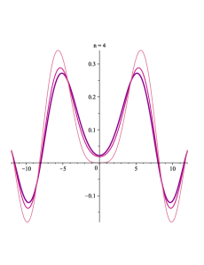
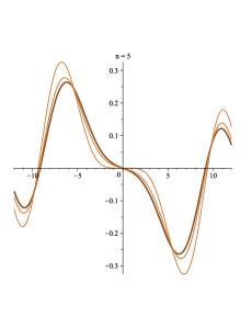
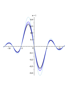
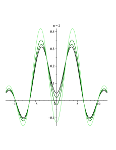
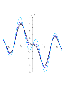
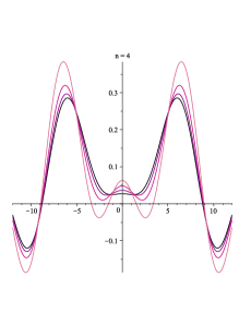
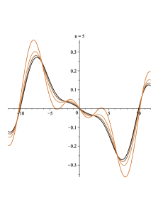
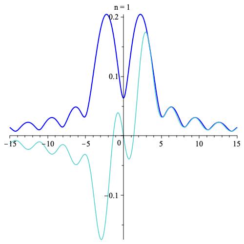
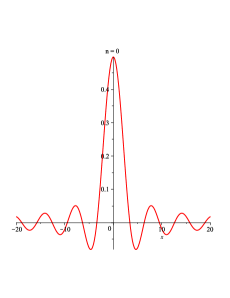
Figure 6.1: The first six functions ฯ†nโŸจ1โŸฉsuperscriptsubscript๐œ‘๐‘›delimited-โŸจโŸฉ1\varphi_{n}^{\langle 1\rangle} for the Legendre weight.

In Fig.ย 6.1 we have computed ฯ†0โŸจ1โŸฉ,โ€ฆ,ฯ†5โŸจ1โŸฉsuperscriptsubscript๐œ‘0delimited-โŸจโŸฉ1โ€ฆsuperscriptsubscript๐œ‘5delimited-โŸจโŸฉ1\varphi_{0}^{\langle 1\rangle},\ldots,\varphi_{5}^{\langle 1\rangle} numerically. Like other transformed functions (1.1) or (2.3), the ฯ†nโŸจ1โŸฉsuperscriptsubscript๐œ‘๐‘›delimited-โŸจโŸฉ1\varphi_{n}^{\langle 1\rangle}s seem to be endowed with a wealth of structural features and regularities which have been discussed briefly (for (1.1)) in (?) but overall are a subject for future research.

6.3 Sobolevโ€“Legendre cascades

We revisit the essence of Subsections 3.1.1โ€“2, except that the range of integration is now [โˆ’1,1]11[-1,1]. Firstly, we set w=ฯ‡(โˆ’1,1)๐‘คsubscript๐œ’11w=\chi_{(-1,1)}, let pnsubscript๐‘๐‘›p_{n} be the (orthonormalised) Legendre polynomials and, for every sโˆˆโ„ค+๐‘ subscriptโ„คs\in\mbox{\Bbb Z}_{+} set

ฯ†nโŸจsโŸฉโ€‹(x)=in2โ€‹ฯ€โ€‹โˆซโˆ’11pnโ€‹(ฮพ)โ€‹(โˆ‘โ„“=0sฮพ2โ€‹โ„“)โˆ’1/2โ€‹eiโ€‹xโ€‹ฮพโ€‹dฮพ,nโˆˆโ„ค+.formulae-sequencesuperscriptsubscript๐œ‘๐‘›delimited-โŸจโŸฉ๐‘ ๐‘ฅsuperscripti๐‘›2๐œ‹superscriptsubscript11subscript๐‘๐‘›๐œ‰superscriptsuperscriptsubscriptโ„“0๐‘ superscript๐œ‰2โ„“12superscriptei๐‘ฅ๐œ‰differential-d๐œ‰๐‘›subscriptโ„ค\varphi_{n}^{\langle s\rangle}(x)=\frac{{\mathrm{i}}^{n}}{\sqrt{2\pi}}\int_{-1}^{1}p_{n}(\xi)\left(\sum_{\ell=0}^{s}\xi^{2\ell}\!\right)^{\!-1/2}\mathrm{e}^{{\mathrm{i}}x\xi}\,\mathrm{d}\xi,\qquad n\in\mbox{\Bbb Z}_{+}. (6.2)

Secondly, we might define wsโ€‹(ฮพ)=ฯ‡(โˆ’1,1)โ€‹(ฮพ)โ€‹โˆ‘โ„“=0sฮพ2โ€‹โ„“subscript๐‘ค๐‘ ๐œ‰subscript๐œ’11๐œ‰superscriptsubscriptโ„“0๐‘ superscript๐œ‰2โ„“w_{s}(\xi)=\chi_{(-1,1)}(\xi)\sum_{\ell=0}^{s}\xi^{2\ell}, sโˆˆโ„ค+๐‘ subscriptโ„คs\in\mbox{\Bbb Z}_{+}, and set

ฯ†n[s]โ€‹(x)=in2โ€‹ฯ€โ€‹โˆซโˆ’11pn[s]โ€‹(ฮพ)โ€‹eiโ€‹xโ€‹ฮพโ€‹dฮพ,nโˆˆโ„ค+,formulae-sequencesuperscriptsubscript๐œ‘๐‘›delimited-[]๐‘ ๐‘ฅsuperscripti๐‘›2๐œ‹superscriptsubscript11subscriptsuperscript๐‘delimited-[]๐‘ ๐‘›๐œ‰superscriptei๐‘ฅ๐œ‰differential-d๐œ‰๐‘›subscriptโ„ค\varphi_{n}^{[s]}(x)=\frac{{\mathrm{i}}^{n}}{\sqrt{2\pi}}\int_{-1}^{1}p^{[s]}_{n}(\xi)\mathrm{e}^{{\mathrm{i}}x\xi}\,\mathrm{d}\xi,\qquad n\in\mbox{\Bbb Z}_{+}, (6.3)

where {pn[s]}nโˆˆโ„ค+subscriptsuperscriptsubscript๐‘๐‘›delimited-[]๐‘ ๐‘›subscriptโ„ค\{p_{n}^{[s]}\}_{n\in\mbox{\sBbb Z}_{+}} is the orthonormal polynomial system corresponding to the weight wssubscript๐‘ค๐‘ w_{s}. It follows at once from Theoremย 2 that

โˆ‘โ„“=0sโˆซโˆ’โˆžโˆždโ„“โ€‹ฯ†mโŸจsโŸฉโ€‹(x)dโ€‹xโ„“โ€‹dโ„“โ€‹ฯ†nโŸจsโŸฉโ€‹(x)dโ€‹xโ„“โ€‹dx=โˆ‘โ„“=0sโˆซโˆ’โˆžโˆždโ„“โ€‹ฯ†m[s]โ€‹(x)dโ€‹xโ„“โ€‹dโ„“โ€‹ฯ†n[s]โ€‹(x)dโ€‹xโ„“โ€‹dx=ฮดm,nsuperscriptsubscriptโ„“0๐‘ superscriptsubscriptsuperscriptdโ„“superscriptsubscript๐œ‘๐‘šdelimited-โŸจโŸฉ๐‘ ๐‘ฅdsuperscript๐‘ฅโ„“superscriptdโ„“superscriptsubscript๐œ‘๐‘›delimited-โŸจโŸฉ๐‘ ๐‘ฅdsuperscript๐‘ฅโ„“differential-d๐‘ฅsuperscriptsubscriptโ„“0๐‘ superscriptsubscriptsuperscriptdโ„“superscriptsubscript๐œ‘๐‘šdelimited-[]๐‘ ๐‘ฅdsuperscript๐‘ฅโ„“superscriptdโ„“superscriptsubscript๐œ‘๐‘›delimited-[]๐‘ ๐‘ฅdsuperscript๐‘ฅโ„“differential-d๐‘ฅsubscript๐›ฟ๐‘š๐‘›\sum_{\ell=0}^{s}\int_{-\infty}^{\infty}\frac{\,\mathrm{d}^{\ell}\varphi_{m}^{\langle s\rangle}(x)}{\,\mathrm{d}x^{\ell}}\frac{\,\mathrm{d}^{\ell}\varphi_{n}^{\langle s\rangle}(x)}{\,\mathrm{d}x^{\ell}}\,\mathrm{d}x=\sum_{\ell=0}^{s}\int_{-\infty}^{\infty}\frac{\,\mathrm{d}^{\ell}\varphi_{m}^{[s]}(x)}{\,\mathrm{d}x^{\ell}}\frac{\,\mathrm{d}^{\ell}\varphi_{n}^{[s]}(x)}{\,\mathrm{d}x^{\ell}}\,\mathrm{d}x=\delta_{m,n}

for all m,nโˆˆโ„ค+๐‘š๐‘›subscriptโ„คm,n\in\mbox{\Bbb Z}_{+} and both {ฯ†nโŸจsโŸฉ}nโˆˆโ„ค+subscriptsuperscriptsubscript๐œ‘๐‘›delimited-โŸจโŸฉ๐‘ ๐‘›subscriptโ„ค\{\varphi_{n}^{\langle s\rangle}\}_{n\in\mbox{\sBbb Z}_{+}} and {ฯ†n[s]}nโˆˆโ„ค+subscriptsuperscriptsubscript๐œ‘๐‘›delimited-[]๐‘ ๐‘›subscriptโ„ค\{\varphi_{n}^{[s]}\}_{n\in\mbox{\sBbb Z}_{+}} are orthonormal sets in Hsโ€‹(โ„)superscriptH๐‘ โ„\mathrm{H}^{s}(\mbox{\Bbb R}). Of course, neither is dense in the Sobolev space because their Fourier spectra are restricted to [โˆ’1,1]11[-1,1] โ€“ they are dense in an obvious generalisation of Paleyโ€“Wiener spaces to the realm of Sobolev spaces. The systems (6.2) and (6.3) are the Sobolevโ€“Legendre cascades of the first and the second kind, respectively.

We recall a major practical difference between the two cascades: except for the case s=0๐‘ 0s=0 (when ฯ†nโŸจ0โŸฉ=ฯ†n[0]subscriptsuperscript๐œ‘delimited-โŸจโŸฉ0๐‘›subscriptsuperscript๐œ‘delimited-[]0๐‘›\varphi^{\langle 0\rangle}_{n}=\varphi^{[0]}_{n} has been given in (6.1)), ฯ†nโŸจsโŸฉsuperscriptsubscript๐œ‘๐‘›delimited-โŸจโŸฉ๐‘ \varphi_{n}^{\langle s\rangle} is unknown in an explicit form while ฯ†n[s]superscriptsubscript๐œ‘๐‘›delimited-[]๐‘ \varphi_{n}^{[s]}, being an integral in [โˆ’1,1]11[-1,1] of a polynomial times eiโ€‹xโ€‹ฮพsuperscriptei๐‘ฅ๐œ‰\mathrm{e}^{{\mathrm{i}}x\xi}, can be computed at great ease and is a linear combination of spherical Bessel functions. Consequently, in the sequel we focus on the Sobolevโ€“Lagendre cascade of the second kind.
Refer to caption
Refer to caption
Refer to caption
Refer to caption
Refer to caption
Refer to caption
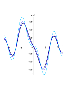
Figure 6.2: The Sobolevโ€“Legendre cascade of the second kind: The first six functions ฯ†n[s]superscriptsubscript๐œ‘๐‘›delimited-[]๐‘ \varphi_{n}^{[s]} for s=0,1,2๐‘ 012s=0,1,2: increasing s๐‘ s corresponds to increasing line thickness and darker hue.

Fig.ย 6.2 displays the beginning (that is, s=0,1,2๐‘ 012s=0,1,2) of the cascade of the second kind. The obvious observation is that ฯ†0[s]subscriptsuperscript๐œ‘delimited-[]๐‘ 0\varphi^{[s]}_{0} is a scalar multiple of ฯ†0[0]subscriptsuperscript๐œ‘delimited-[]00\varphi^{[0]}_{0} and the same is true for ฯ†1[s]superscriptsubscript๐œ‘1delimited-[]๐‘ \varphi_{1}^{[s]} and ฯ†1[0]superscriptsubscript๐œ‘1delimited-[]0\varphi_{1}^{[0]}, respectively. This follows from (6.3) because p0[s]superscriptsubscript๐‘0delimited-[]๐‘ p_{0}^{[s]} is a constant, while p1[s]superscriptsubscript๐‘1delimited-[]๐‘ p_{1}^{[s]} is a scalar multiple of ฮพ๐œ‰\xi. Another obvious indication is that, as s๐‘ s grows, ฯ†n[s]superscriptsubscript๐œ‘๐‘›delimited-[]๐‘ \varphi_{n}^{[s]} converges pointwise to a function ฯ†n[โˆž]superscriptsubscript๐œ‘๐‘›delimited-[]\varphi_{n}^{[\infty]} yet this might be less interesting than it appears. In particular,

Lemma 11

ฯ†n[โˆž]โ‰ก0superscriptsubscript๐œ‘๐‘›delimited-[]0\varphi_{n}^{[\infty]}\equiv 0.

Proofโ€ƒLet

us=โˆซโˆ’11โˆ‘โ„“=0sฮพ2โ€‹โ„“โ€‹dโ€‹ฮพ,sโˆˆโ„ค+.formulae-sequencesubscript๐‘ข๐‘ superscriptsubscript11superscriptsubscriptโ„“0๐‘ superscript๐œ‰2โ„“d๐œ‰๐‘ subscriptโ„คu_{s}=\int_{-1}^{1}\sum_{\ell=0}^{s}\xi^{2\ell}\,\mathrm{d}\xi,\qquad s\in\mbox{\Bbb Z}_{+}.

Then p0[0]โ‰ก1/u2superscriptsubscript๐‘0delimited-[]01subscript๐‘ข2p_{0}^{[0]}\equiv 1/\sqrt{u_{2}} and, by (6.3),

ฯ†0[s]โ€‹(x)=2ฯ€โ€‹usโ€‹sinโกxx.superscriptsubscript๐œ‘0delimited-[]๐‘ ๐‘ฅ2๐œ‹subscript๐‘ข๐‘ ๐‘ฅ๐‘ฅ\varphi_{0}^{[s]}(x)=\sqrt{\frac{2}{\pi u_{s}}}\frac{\sin x}{x}.

But

us=โˆ‘โ„“=0s1โ„“+12โŸถโ„“โ†’โˆžโˆžsubscript๐‘ข๐‘ superscriptsubscriptโ„“0๐‘ 1โ„“12superscriptโŸถโ†’โ„“u_{s}=\sum_{\ell=0}^{s}\frac{1}{\ell+\frac{1}{2}}\stackrel{{\scriptstyle\ell\rightarrow\infty}}{{\longrightarrow}}\infty

and the lemma follows. ย ย ย ย ย ย  โ–กโ–ก\Box

Alternatively, limsโ†’โˆžw[s]โ€‹(ฮพ)=(1โˆ’ฮพ2)โˆ’1โ€‹ฯ‡(โˆ’1,1)โˆ‰L2โ€‹(โ„)subscriptโ†’๐‘ superscript๐‘คdelimited-[]๐‘ ๐œ‰superscript1superscript๐œ‰21subscript๐œ’11subscriptL2โ„\lim_{s\rightarrow\infty}w^{[s]}(\xi)=(1-\xi^{2})^{-1}\chi_{(-1,1)}\not\in\mathrm{L}_{2}(\mbox{\Bbb R}). An obvious remedy, which we do not pursue in this paper, is to consider the weight wsโ€‹(ฮพ)=โˆ‘โ„“=0sฯƒโ„“โ€‹ฮพ2โ€‹โ„“subscript๐‘ค๐‘ ๐œ‰superscriptsubscriptโ„“0๐‘ superscript๐œŽโ„“superscript๐œ‰2โ„“w_{s}(\xi)=\sum_{\ell=0}^{s}\sigma^{\ell}\xi^{2\ell} for some ฯƒโˆˆ(0,1)๐œŽ01\sigma\in(0,1).

6.4 The Sobolev-ultraspherical cascade of the second kind

We construct a cascade of the second kind based on the ultraspherical weight w[0]โ€‹(ฮพ)=(1โˆ’ฮพ2)โ€‹ฯ‡(โˆ’1,1)โ€‹(ฮพ)superscript๐‘คdelimited-[]0๐œ‰1superscript๐œ‰2subscript๐œ’11๐œ‰w^{[0]}(\xi)=(1-\xi^{2})\chi_{(-1,1)}(\xi). Therefore

w[s]โ€‹(ฮพ)=w[0]โ€‹(ฮพ)โ€‹โˆ‘โ„“=0sฮพ2โ€‹โ„“=(1โˆ’ฮพ2โ€‹s+2)โ€‹ฯ‡(โˆ’1,1),sโˆˆโ„ค+formulae-sequencesuperscript๐‘คdelimited-[]๐‘ ๐œ‰superscript๐‘คdelimited-[]0๐œ‰superscriptsubscriptโ„“0๐‘ superscript๐œ‰2โ„“1superscript๐œ‰2๐‘ 2subscript๐œ’11๐‘ subscriptโ„คw^{[s]}(\xi)=w^{[0]}(\xi)\sum_{\ell=0}^{s}\xi^{2\ell}=(1-\xi^{2s+2})\chi_{(-1,1)},\qquad s\in\mbox{\Bbb Z}_{+}

and, as sโ†’โˆžโ†’๐‘ s\rightarrow\infty, w[s]superscript๐‘คdelimited-[]๐‘ w^{[s]} converges weakly to the Legendre weight.
Refer to caption
Refer to caption
Refer to caption
Refer to caption
Refer to caption
Refer to caption
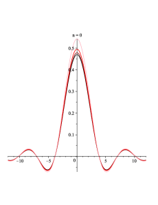
Figure 6.3: The Sobolevโ€“ultrasperical cascade: The first six functions ฯ†n[s]superscriptsubscript๐œ‘๐‘›delimited-[]๐‘ \varphi_{n}^{[s]} for s=0,1,2,3๐‘ 0123s=0,1,2,3: increasing s๐‘ s corresponds to darker hue.

In Fig.ย 6.3 we display the functions ฯ†n[0],โ€ฆ,ฯ†n[3]superscriptsubscript๐œ‘๐‘›delimited-[]0โ€ฆsuperscriptsubscript๐œ‘๐‘›delimited-[]3\varphi_{n}^{[0]},\ldots,\varphi_{n}^{[3]} for n=0,1,โ€ฆ,5๐‘›01โ€ฆ5n=0,1,\ldots,5. While the convergence to a limit in each figure is quite persuasive, we must beware of โ€˜proof by pictureโ€™: convergence is equally pictorially persuasive in Fig.ย 6.2 where, as we have already seen, it need not take place.

7 Non-symmetric measures

The most obvious non-symmetric weight function is the Laguerre weight wโ€‹(ฮพ)=eโˆ’ฮพโ€‹ฯ‡[0,โˆž)โ€‹(ฮพ)๐‘ค๐œ‰superscripte๐œ‰subscript๐œ’0๐œ‰w(\xi)=\mathrm{e}^{-\xi}\chi_{[0,\infty)}(\xi). In that case the ฯ†nsubscript๐œ‘๐‘›\varphi_{n}s are the Malmquistโ€“Takenaka functions, which have a particularly neat form,

ฯ†nโ€‹(x)=2ฯ€โ€‹inโ€‹(1+2โ€‹iโ€‹x)n(1โˆ’2โ€‹iโ€‹x)n+1,nโˆˆโ„ค+,formulae-sequencesubscript๐œ‘๐‘›๐‘ฅ2๐œ‹superscripti๐‘›superscript12i๐‘ฅ๐‘›superscript12i๐‘ฅ๐‘›1๐‘›subscriptโ„ค\varphi_{n}(x)=\sqrt{\frac{2}{\pi}}{\mathrm{i}}^{n}\frac{(1+2{\mathrm{i}}x)^{n}}{(1-2{\mathrm{i}}x)^{n+1}},\qquad n\in\mbox{\Bbb Z}_{+}, (7.1)

(?), and they are dense in ๐’ซโ€‹๐’ฒ[0,โˆž)โ€‹(โ„)๐’ซsubscript๐’ฒ0โ„\mathcal{PW}_{[0,\infty)}(\mbox{\Bbb R}). It is possible to extend them to a system dense in all of L2โ€‹(โ„)subscriptL2โ„\mathrm{L}_{2}(\mbox{\Bbb R}) by melding them with another system, generated by the mirror image of the Laguerre weight, eฮพโ€‹ฯ‡(โˆ’โˆž,0]โ€‹(ฮพ)superscripte๐œ‰subscript๐œ’0๐œ‰\mathrm{e}^{\xi}\chi_{(-\infty,0]}(\xi): together we obtain the same system as (7.1), except that now n๐‘›n ranges over all of โ„ค.

It is, of course, perfectly possible for a system with a non-symmetric measure to be dense in L2โ€‹(โ„)subscriptL2โ„\mathrm{L}_{2}(\mbox{\Bbb R}), provided that the support of w๐‘คw is all of โ„: an example is the Hermite-type weight wโ€‹(ฮพ)=(1โˆ’ฮพ)2โ€‹eโˆ’ฮพ2๐‘ค๐œ‰superscript1๐œ‰2superscriptesuperscript๐œ‰2w(\xi)=(1-\xi)^{2}\mathrm{e}^{-\xi^{2}}.

7.1 Shifted Hermite weight

Letting ฯโˆˆโ„๐œŒโ„\rho\in\mbox{\Bbb R}, we consider the weight wโ€‹(ฮพ)=eโˆ’(ฮพโˆ’ฯ)2๐‘ค๐œ‰superscriptesuperscript๐œ‰๐œŒ2w(\xi)=\mathrm{e}^{-(\xi-\rho)^{2}}. The underlying orthonormal polynomials are pnโ€‹(ฮพ)=H~nโ€‹(ฮพโˆ’ฯ)subscript๐‘๐‘›๐œ‰subscript~H๐‘›๐œ‰๐œŒp_{n}(\xi)=\tilde{\mathrm{H}}_{n}(\xi-\rho), where H~nsubscript~H๐‘›\tilde{\mathrm{H}}_{n} is the orthonormalised Hermite polynomial, H~n=Hn/2nโ€‹n!โ€‹ฯ€subscript~H๐‘›subscriptH๐‘›superscript2๐‘›๐‘›๐œ‹\tilde{\mathrm{H}}_{n}=\mathrm{H}_{n}/\sqrt{2^{n}n!\sqrt{\pi}}. Therefore, seeking H1โ€‹(โ„)superscriptH1โ„\mathrm{H}^{1}(\mbox{\Bbb R}) orthogonality,

ฯ†nโŸจ0โŸฉโ€‹(x,ฯ)superscriptsubscript๐œ‘๐‘›delimited-โŸจโŸฉ0๐‘ฅ๐œŒ\displaystyle\varphi_{n}^{\langle 0\rangle}(x,\rho) =\displaystyle= in2โ€‹ฯ€โ€‹โˆซโˆ’โˆžโˆžH~nโ€‹(ฮพโˆ’ฯ)โ€‹eโˆ’(ฮพโˆ’ฯ)2/2+iโ€‹xโ€‹ฮพโ€‹dฮพ=eiโ€‹ฯโ€‹xโ€‹ฯ†nโŸจ0โŸฉโ€‹(x,0),superscripti๐‘›2๐œ‹superscriptsubscriptsubscript~H๐‘›๐œ‰๐œŒsuperscriptesuperscript๐œ‰๐œŒ22i๐‘ฅ๐œ‰differential-d๐œ‰superscriptei๐œŒ๐‘ฅsuperscriptsubscript๐œ‘๐‘›delimited-โŸจโŸฉ0๐‘ฅ0\displaystyle\frac{{\mathrm{i}}^{n}}{\sqrt{2\pi}}\int_{-\infty}^{\infty}\tilde{\mathrm{H}}_{n}(\xi-\rho)\mathrm{e}^{-(\xi-\rho)^{2}/2+{\mathrm{i}}x\xi}\,\mathrm{d}\xi=\mathrm{e}^{{\mathrm{i}}\rho x}\varphi_{n}^{\langle 0\rangle}(x,0),
ฯ†nโŸจ1โŸฉโ€‹(x,ฯ)superscriptsubscript๐œ‘๐‘›delimited-โŸจโŸฉ1๐‘ฅ๐œŒ\displaystyle\varphi_{n}^{\langle 1\rangle}(x,\rho) =\displaystyle= in2โ€‹ฯ€โ€‹โˆซโˆ’โˆžโˆžH~nโ€‹(ฮพโˆ’ฯ)โ€‹eโˆ’(ฮพโˆ’ฯ)2/2+iโ€‹xโ€‹ฮพ1+ฮพ2โ€‹dฮพ,nโˆˆโ„ค+.superscripti๐‘›2๐œ‹superscriptsubscriptsubscript~H๐‘›๐œ‰๐œŒsuperscriptesuperscript๐œ‰๐œŒ22i๐‘ฅ๐œ‰1superscript๐œ‰2differential-d๐œ‰๐‘›subscriptโ„ค\displaystyle\frac{{\mathrm{i}}^{n}}{\sqrt{2\pi}}\int_{-\infty}^{\infty}\tilde{\mathrm{H}}_{n}(\xi-\rho)\frac{\mathrm{e}^{-(\xi-\rho)^{2}/2+{\mathrm{i}}x\xi}}{\sqrt{1+\xi^{2}}}\,\mathrm{d}\xi,\qquad n\in\mbox{\Bbb Z}_{+}.

It is easy to verify that

ฯ†nโŸจ0โŸฉโ€‹(x,ฯ)=eiโ€‹ฯโ€‹xโ€‹ฯ†0โŸจ0โŸฉโ€‹(x,0),x,ฯโˆˆโ„.formulae-sequencesuperscriptsubscript๐œ‘๐‘›delimited-โŸจโŸฉ0๐‘ฅ๐œŒsuperscriptei๐œŒ๐‘ฅsuperscriptsubscript๐œ‘0delimited-โŸจโŸฉ0๐‘ฅ0๐‘ฅ๐œŒโ„\varphi_{n}^{\langle 0\rangle}(x,\rho)=\mathrm{e}^{{\mathrm{i}}\rho x}\varphi_{0}^{\langle 0\rangle}(x,0),\qquad x,\rho\in\mbox{\Bbb R}.

Thus, ฯ†nโŸจ0โŸฉ=ฯ†n[0]superscriptsubscript๐œ‘๐‘›delimited-โŸจโŸฉ0superscriptsubscript๐œ‘๐‘›delimited-[]0\varphi_{n}^{\langle 0\rangle}=\varphi_{n}^{[0]} is merely a complex-valued rotation of the standard Hermite function. The situation is more intriguing with regard to ฯ†nโŸจ1โŸฉsuperscriptsubscript๐œ‘๐‘›delimited-โŸจโŸฉ1\varphi_{n}^{\langle 1\rangle}. Shifting the variable of integration,

ฯ†nโŸจ1โŸฉโ€‹(x,ฯ)=inโ€‹eiโ€‹ฯโ€‹x2โ€‹ฯ€โ€‹โˆซโˆ’โˆžโˆžH~nโ€‹(ฮพ)โ€‹eโˆ’ฮพ21+(ฯƒ+ฮพ)2โ€‹eiโ€‹xโ€‹ฮพโ€‹dฮพ.superscriptsubscript๐œ‘๐‘›delimited-โŸจโŸฉ1๐‘ฅ๐œŒsuperscripti๐‘›superscriptei๐œŒ๐‘ฅ2๐œ‹superscriptsubscriptsubscript~H๐‘›๐œ‰superscriptesuperscript๐œ‰21superscript๐œŽ๐œ‰2superscriptei๐‘ฅ๐œ‰differential-d๐œ‰\varphi_{n}^{\langle 1\rangle}(x,\rho)=\frac{{\mathrm{i}}^{n}\mathrm{e}^{{\mathrm{i}}\rho x}}{\sqrt{2\pi}}\int_{-\infty}^{\infty}\tilde{\mathrm{H}}_{n}(\xi)\sqrt{\frac{\mathrm{e}^{-\xi^{2}}}{1+(\sigma+\xi)^{2}}}\mathrm{e}^{{\mathrm{i}}x\xi}\,\mathrm{d}\xi.

On the face of it, we recover an expression similar to (2.3), except that vโ€‹(ฮพ)=1+(ฯƒ+ฮพ)2๐‘ฃ๐œ‰1superscript๐œŽ๐œ‰2v(\xi)=1+(\sigma+\xi)^{2} is not an even function and does not define a Sobolev inner product.
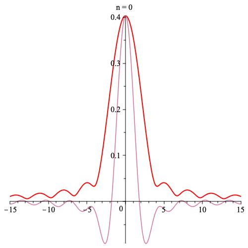
Refer to caption
Refer to caption
Refer to caption
Refer to caption
Refer to caption
Refer to caption
Figure 7.1: Shifted Sobolevโ€“Hermite functions: |ฯ†nโŸจ1โŸฉโ€‹(x,1)|superscriptsubscript๐œ‘๐‘›delimited-โŸจโŸฉ1๐‘ฅ1|\varphi_{n}^{\langle 1\rangle}(x,1)| in thicker line and darker colour and Reโ€‹ฯ†nโŸจ1โŸฉโ€‹(x,1)Resuperscriptsubscript๐œ‘๐‘›delimited-โŸจโŸฉ1๐‘ฅ1\mathrm{Re}\,\varphi_{n}^{\langle 1\rangle}(x,1), for n=0,โ€ฆ,5๐‘›0โ€ฆ5n=0,\ldots,5.

Fig.ย 7.1 displays the absolute and real values of the complex-valued functions ฯ†nโŸจ1โŸฉsuperscriptsubscript๐œ‘๐‘›delimited-โŸจโŸฉ1\varphi_{n}^{\langle 1\rangle}.

7.2 The Laguerre weight

7.2.1 Sobolevโ€“Laguerre functions of first kind

Let wโ€‹(ฮพ)=eโˆ’ฮพโ€‹ฯ‡[0,โˆž)โ€‹(ฮพ)๐‘ค๐œ‰superscripte๐œ‰subscript๐œ’0๐œ‰w(\xi)=\mathrm{e}^{-\xi}\chi_{[0,\infty)}(\xi), a Laguerre weight. Thus, the ฯ†nโŸจ0โŸฉsuperscriptsubscript๐œ‘๐‘›delimited-โŸจโŸฉ0\varphi_{n}^{\langle 0\rangle}s are Malmquistโ€“Takenaka functions (7.1), which we need to complement with their โ€˜reflectionsโ€™ for nโˆˆโˆ’โ„•๐‘›โ„•n\in-\mbox{\Bbb N} to form a system dense in L2โ€‹(โ„)subscriptL2โ„\mathrm{L}_{2}(\mbox{\Bbb R}). By similar token, we need to complement ฯ†nโŸจ1โŸฉsuperscriptsubscript๐œ‘๐‘›delimited-โŸจโŸฉ1\varphi_{n}^{\langle 1\rangle}s, nโˆˆโ„ค+๐‘›subscriptโ„คn\in\mbox{\Bbb Z}_{+}, with functions generated with wโ€‹(ฮพ)=eฮพโ€‹ฯ‡(โˆ’โˆž,0]โ€‹(ฮพ)๐‘ค๐œ‰superscripte๐œ‰subscript๐œ’0๐œ‰w(\xi)=\mathrm{e}^{\xi}\chi_{(-\infty,0]}(\xi) (and indexed by nโˆˆโˆ’โ„•๐‘›โ„•n\in-\mbox{\Bbb N}) to attain completeness in H1โ€‹(โ„)superscriptH1โ„\mathrm{H}^{1}(\mbox{\Bbb R}).

It is possible to compute individual ฯ†nโŸจ1โŸฉsuperscriptsubscript๐œ‘๐‘›delimited-โŸจโŸฉ1\varphi_{n}^{\langle 1\rangle}s explicitly in terms of Bessel functions of the second kind (a.k.a.ย Weber functions) YnsubscriptY๐‘›\mathrm{Y}_{n} (?, 10.2.4) and Struve functions ๐‡nsubscript๐‡๐‘›{\bf H}_{n} (?, 11.2.1). We first let

z=12โˆ’iโ€‹x,gโ€‹(z)=Y0โ€‹(z)โˆ’๐‡0โ€‹(z).formulae-sequence๐‘ง12i๐‘ฅ๐‘”๐‘งsubscriptY0๐‘งsubscript๐‡0๐‘งz=\frac{1}{2}-{\mathrm{i}}x,\qquad g(z)=\mathrm{Y}_{0}(z)-{\bf H}_{0}(z).

The functions ฯ†nsubscript๐œ‘๐‘›\varphi_{n} can be represented explicitly as linear combinations of derivatives of the function g๐‘”g.

Lemma 12

The explicit form of the functions ฯ†nโŸจ1โŸฉsuperscriptsubscript๐œ‘๐‘›delimited-โŸจโŸฉ1\varphi_{n}^{\langle 1\rangle} is

ฯ†nโŸจ1โŸฉโ€‹(x)=โˆ’2โ€‹ฯ€4โ€‹inโ€‹โˆ‘โ„“=0n(nโ„“)โ€‹1โ„“!โ€‹g(โ„“)โ€‹(12โˆ’iโ€‹x),nโˆˆโ„ค+,formulae-sequencesuperscriptsubscript๐œ‘๐‘›delimited-โŸจโŸฉ1๐‘ฅ2๐œ‹4superscripti๐‘›superscriptsubscriptโ„“0๐‘›binomial๐‘›โ„“1โ„“superscript๐‘”โ„“12i๐‘ฅ๐‘›subscriptโ„ค\varphi_{n}^{\langle 1\rangle}(x)=-\frac{\sqrt{2\pi}}{4}{\mathrm{i}}^{n}\sum_{\ell=0}^{n}{n\choose\ell}\frac{1}{\ell!}g^{(\ell)}\!\!\left(\frac{1}{2}-{\mathrm{i}}x\right)\!,\qquad n\in\mbox{\Bbb Z}_{+}, (7.2)

while ฯ†โˆ’nโˆ’1โŸจ1โŸฉโ€‹(x)=(โˆ’1)n+1โ€‹ฯ†nโŸจ1โŸฉโ€‹(x)ยฏsuperscriptsubscript๐œ‘๐‘›1delimited-โŸจโŸฉ1๐‘ฅsuperscript1๐‘›1ยฏsuperscriptsubscript๐œ‘๐‘›delimited-โŸจโŸฉ1๐‘ฅ\varphi_{-n-1}^{\langle 1\rangle}(x)=(-1)^{n+1}\overline{\varphi_{n}^{\langle 1\rangle}(x)}, nโˆˆโ„ค+๐‘›subscriptโ„คn\in\mbox{\Bbb Z}_{+}.

Proofโ€ƒLetting

ฮทnโ€‹(x)=12โ€‹ฯ€โ€‹โˆซ0โˆžฮพnโ€‹eโˆ’ฮพ/2+iโ€‹xโ€‹ฮพ1+ฮพ2โ€‹dฮพ,nโˆˆโ„ค+,formulae-sequencesubscript๐œ‚๐‘›๐‘ฅ12๐œ‹superscriptsubscript0superscript๐œ‰๐‘›superscripte๐œ‰2i๐‘ฅ๐œ‰1superscript๐œ‰2differential-d๐œ‰๐‘›subscriptโ„ค\eta_{n}(x)=\frac{1}{\sqrt{2\pi}}\int_{0}^{\infty}\xi^{n}\frac{\mathrm{e}^{-\xi/2+{\mathrm{i}}x\xi}}{\sqrt{1+\xi^{2}}}\,\mathrm{d}\xi,\qquad n\in\mbox{\Bbb Z}_{+},

we compute the generating function

Gโ€‹(x,T)๐บ๐‘ฅ๐‘‡\displaystyle G(x,T) =\displaystyle= โˆ‘n=0โˆžฮทnโ€‹(x)n!โ€‹Tn=12โ€‹ฯ€โ€‹โˆซ0โˆž11+ฮพ2โ€‹expโก(โˆ’ฮพ2+Tโ€‹ฮพ+iโ€‹xโ€‹ฮพ)โ€‹dฮพsuperscriptsubscript๐‘›0subscript๐œ‚๐‘›๐‘ฅ๐‘›superscript๐‘‡๐‘›12๐œ‹superscriptsubscript011superscript๐œ‰2๐œ‰2๐‘‡๐œ‰i๐‘ฅ๐œ‰differential-d๐œ‰\displaystyle\sum_{n=0}^{\infty}\frac{\eta_{n}(x)}{n!}T^{n}=\frac{1}{\sqrt{2\pi}}\int_{0}^{\infty}\frac{1}{\sqrt{1+\xi^{2}}}\exp\!\left(-\frac{\xi}{2}+T\xi+{\mathrm{i}}x\xi\right)\!\,\mathrm{d}\xi
=\displaystyle= โˆ’2โ€‹ฯ€4โ€‹[Y0โ€‹(12โˆ’iโ€‹xโˆ’T)โˆ’๐‡0โ€‹(12โˆ’iโ€‹xโˆ’T)].2๐œ‹4delimited-[]subscriptY012i๐‘ฅ๐‘‡subscript๐‡012i๐‘ฅ๐‘‡\displaystyle-\frac{\sqrt{2\pi}}{4}\left[\mathrm{Y}_{0}\!\left(\frac{1}{2}-{\mathrm{i}}x-T\right)-{\bf H}_{0}\!\left(\frac{1}{2}-{\mathrm{i}}x-T\right)\!\right]\!.

Therefore

ฮทnโ€‹(x)=โˆ‚nGโ€‹(x,T)โˆ‚Tnโ€‹ย T=0=(โˆ’1)n+1โ€‹2โ€‹ฯ€4โ€‹g(n)โ€‹(12โˆ’iโ€‹x),nโˆˆโ„ค+.formulae-sequencesubscript๐œ‚๐‘›๐‘ฅsuperscript๐‘›๐บ๐‘ฅ๐‘‡superscript๐‘‡๐‘›subscriptย ๐‘‡0superscript1๐‘›12๐œ‹4superscript๐‘”๐‘›12i๐‘ฅ๐‘›subscriptโ„ค\eta_{n}(x)=\frac{\partial^{n}G(x,T)}{\partial T^{n}}\,\rule[-8.0pt]{0.75pt}{22.0pt}_{\,T=0}=(-1)^{n+1}\frac{\sqrt{2\pi}}{4}g^{(n)}\!\!\left(\frac{1}{2}-{\mathrm{i}}x\right)\!,\qquad n\in\mbox{\Bbb Z}_{+}.

Laguerre polynomials LnsubscriptL๐‘›\mathrm{L}_{n} are orthonormal and

Lnโ€‹(x)=โˆ‘โ„“=0n(โˆ’1)โ„“โ€‹(nโ„“)โ€‹xโ„“โ„“!,nโˆˆโ„ค+formulae-sequencesubscriptL๐‘›๐‘ฅsuperscriptsubscriptโ„“0๐‘›superscript1โ„“binomial๐‘›โ„“superscript๐‘ฅโ„“โ„“๐‘›subscriptโ„ค\mathrm{L}_{n}(x)=\sum_{\ell=0}^{n}(-1)^{\ell}{n\choose\ell}\frac{x^{\ell}}{\ell!},\qquad n\in\mbox{\Bbb Z}_{+}

(?, 18.5.12) and it follows from Theoremย 1 that

ฯ†nโŸจ1โŸฉโ€‹(x)=in2โ€‹ฯ€โ€‹โˆซ0โˆžLnโ€‹(ฮพ)โ€‹eโˆ’ฮพ/2+iโ€‹xโ€‹ฮพ1+ฮพ2โ€‹dฮพ=inโ€‹โˆ‘โ„“=0n(โˆ’1)โ„“โ€‹(nโ„“)โ€‹ฮทโ„“โ€‹(x)โ„“!,superscriptsubscript๐œ‘๐‘›delimited-โŸจโŸฉ1๐‘ฅsuperscripti๐‘›2๐œ‹superscriptsubscript0subscriptL๐‘›๐œ‰superscripte๐œ‰2i๐‘ฅ๐œ‰1superscript๐œ‰2differential-d๐œ‰superscripti๐‘›superscriptsubscriptโ„“0๐‘›superscript1โ„“binomial๐‘›โ„“subscript๐œ‚โ„“๐‘ฅโ„“\varphi_{n}^{\langle 1\rangle}(x)=\frac{{\mathrm{i}}^{n}}{\sqrt{2\pi}}\int_{0}^{\infty}\mathrm{L}_{n}(\xi)\frac{\mathrm{e}^{-\xi/2+{\mathrm{i}}x\xi}}{\sqrt{1+\xi^{2}}}\,\mathrm{d}\xi={\mathrm{i}}^{n}\sum_{\ell=0}^{n}(-1)^{\ell}{n\choose\ell}\frac{\eta_{\ell}(x)}{\ell!},

thereby proving (7.2) upon the substitution of the explicit form of ฮทโ„“subscript๐œ‚โ„“\eta_{\ell}.

Extending this to nโ‰คโˆ’1๐‘›1n\leq-1 is trivial. ย ย ย ย ย ย  โ–กโ–ก\Box

Corollary 1

The functions ฯ†nsubscript๐œ‘๐‘›\varphi_{n} for nโˆˆโ„ค+๐‘›subscriptโ„คn\in\mbox{\Bbb Z}_{+} have the generating function

โˆ‘n=0โˆžฯ†nโŸจ1โŸฉโ€‹(x)n!โ€‹tn=โˆ’2โ€‹ฯ€4โ€‹eiโ€‹tโ€‹โˆ‘โ„“=0โˆž(iโ€‹t)โ„“โ„“!2โ€‹g(โ„“)โ€‹(12โˆ’iโ€‹x).superscriptsubscript๐‘›0superscriptsubscript๐œ‘๐‘›delimited-โŸจโŸฉ1๐‘ฅ๐‘›superscript๐‘ก๐‘›2๐œ‹4superscriptei๐‘กsuperscriptsubscriptโ„“0superscripti๐‘กโ„“superscriptโ„“2superscript๐‘”โ„“12i๐‘ฅ\sum_{n=0}^{\infty}\frac{\varphi_{n}^{\langle 1\rangle}(x)}{n!}t^{n}=-\frac{\sqrt{2\pi}}{4}\mathrm{e}^{{\mathrm{i}}t}\sum_{\ell=0}^{\infty}\frac{({\mathrm{i}}t)^{\ell}}{\ell!^{2}}g^{(\ell)}\!\!\left(\frac{1}{2}-{\mathrm{i}}x\right)\!. (7.3)

The proof is elementary, using (7.2). Moreover, (7.3) can be easily extended to

โˆ‘n=โˆ’โˆžโˆžฯ†nโŸจ1โŸฉโ€‹(x)|n|!โ€‹ฮถn=2โ€‹ฯ€4โ€‹[eโˆ’iโ€‹ฮถโˆ’1โ€‹โˆ‘โ„“=0โˆž(โˆ’iโ€‹ฮถโˆ’1)โ„“โ„“!2โ€‹g(โ„“)โ€‹(12+iโ€‹x)โˆ’eiโ€‹ฮถโ€‹โˆ‘โ„“=0โˆž(iโ€‹ฮถ)โ„“โ„“!2โ€‹g(โ„“)โ€‹(12โˆ’iโ€‹x)],superscriptsubscript๐‘›superscriptsubscript๐œ‘๐‘›delimited-โŸจโŸฉ1๐‘ฅ๐‘›superscript๐œ๐‘›2๐œ‹4delimited-[]superscripteisuperscript๐œ1superscriptsubscriptโ„“0superscriptisuperscript๐œ1โ„“superscriptโ„“2superscript๐‘”โ„“12i๐‘ฅsuperscriptei๐œsuperscriptsubscriptโ„“0superscripti๐œโ„“superscriptโ„“2superscript๐‘”โ„“12i๐‘ฅ\sum_{n=-\infty}^{\infty}\!\frac{\varphi_{n}^{\langle 1\rangle}(x)}{|n|!}\zeta^{n}=\frac{\sqrt{2\pi}}{4}\!\left[\mathrm{e}^{-{\mathrm{i}}\zeta^{-1}}\!\sum_{\ell=0}^{\infty}\frac{(-{\mathrm{i}}\zeta^{-1})^{\ell}}{\ell!^{2}}g^{(\ell)}\!\left(\frac{1}{2}\!+\!{\mathrm{i}}x\!\right)-\mathrm{e}^{{\mathrm{i}}\zeta}\sum_{\ell=0}^{\infty}\frac{({\mathrm{i}}\zeta)^{\ell}}{\ell!^{2}}g^{(\ell)}\!\left(\frac{1}{2}\!-\!{\mathrm{i}}x\!\right)\!\right]\!,

which makes sense for |ฮถ|=1๐œ1|\zeta|=1.

Since

z2โ€‹Ynโ€ฒโ€ฒโ€‹(z)+zโ€‹Ynโ€ฒโ€‹(z)+(z2โˆ’n2)โ€‹Ynโ€‹(z)superscript๐‘ง2superscriptsubscriptY๐‘›โ€ฒโ€ฒ๐‘ง๐‘งsuperscriptsubscriptY๐‘›โ€ฒ๐‘งsuperscript๐‘ง2superscript๐‘›2subscriptY๐‘›๐‘ง\displaystyle z^{2}\mathrm{Y}_{n}^{\prime\prime}(z)+z\mathrm{Y}_{n}^{\prime}(z)+(z^{2}-n^{2})\mathrm{Y}_{n}(z) =\displaystyle= 0,0\displaystyle 0,
z2โ€‹๐‡nโ€ฒโ€ฒโ€‹(z)+zโ€‹๐‡nโ€ฒโ€‹(z)+(z2โˆ’n2)โ€‹๐‡nโ€‹(z)superscript๐‘ง2superscriptsubscript๐‡๐‘›โ€ฒโ€ฒ๐‘ง๐‘งsuperscriptsubscript๐‡๐‘›โ€ฒ๐‘งsuperscript๐‘ง2superscript๐‘›2subscript๐‡๐‘›๐‘ง\displaystyle z^{2}{\bf H}_{n}^{\prime\prime}(z)+z{\bf H}_{n}^{\prime}(z)+(z^{2}-n^{2}){\bf H}_{n}(z) =\displaystyle= zn+12nโˆ’1โ€‹ฯ€โ€‹ฮ“โ€‹(n+12)superscript๐‘ง๐‘›1superscript2๐‘›1๐œ‹ฮ“๐‘›12\displaystyle\frac{z^{n+1}}{2^{n-1}\sqrt{\pi}\mathrm{\Gamma}(n+\frac{1}{2})}

(?, 11.10.5 & 11.2.7), it follows that g๐‘”g obeys

zโ€‹gโ€ฒโ€ฒโ€‹(z)+gโ€ฒโ€‹(z)+zโ€‹gโ€‹(z)=โˆ’2ฯ€โ€‹ฮ“โ€‹(12)=โˆ’2ฯ€๐‘งsuperscript๐‘”โ€ฒโ€ฒ๐‘งsuperscript๐‘”โ€ฒ๐‘ง๐‘ง๐‘”๐‘ง2๐œ‹ฮ“122๐œ‹zg^{\prime\prime}(z)+g^{\prime}(z)+zg(z)=-\frac{2}{\sqrt{\pi}\mathrm{\Gamma}(\frac{1}{2})}=-\frac{2}{\pi}

and we can express g(โ„“)superscript๐‘”โ„“g^{(\ell)} as a linear combination of g๐‘”g and gโ€ฒsuperscript๐‘”โ€ฒg^{\prime} with rational coefficients. We do not pursue further this course of action. Functions ฯ†nโŸจsโŸฉsuperscriptsubscript๐œ‘๐‘›delimited-โŸจโŸฉ๐‘ \varphi_{n}^{\langle s\rangle} for sโ‰ฅ2๐‘ 2s\geq 2 (or even the underlying orthogonal polynomials pnโŸจsโŸฉsuperscriptsubscript๐‘๐‘›delimited-โŸจโŸฉ๐‘ p_{n}^{\langle s\rangle}) are no longer available in an explicit form.

7.2.2 Sobolevโ€“Laguerre functions of the second kind

An alternative is to consider the Sobolevโ€“Laguerre cascade of the second kind. While the orthogonal polynomials pn[s]superscriptsubscript๐‘๐‘›delimited-[]๐‘ p_{n}^{[s]} for the weight wsโ€‹(ฮพ)=eโˆ’ฮพโ€‹ฯ‡[0,โˆž)โ€‹โˆ‘โ„“=0sฮพโ„“2subscript๐‘ค๐‘ ๐œ‰superscripte๐œ‰subscript๐œ’0superscriptsubscriptโ„“0๐‘ superscriptsubscript๐œ‰โ„“2w_{s}(\xi)=\mathrm{e}^{-\xi}\chi_{[0,\infty)}\sum_{\ell=0}^{s}\xi_{\ell}^{2} are unknown for sโˆˆโ„•๐‘ โ„•s\in\mbox{\Bbb N}, the underlying moments are trivial to compute and such polynomials can be generated at will. Also the computation of the ฯ†n[s]superscriptsubscript๐œ‘๐‘›delimited-[]๐‘ \varphi_{n}^{[s]}s does not present a problem: for example

ฯ†0[1]โ€‹(x)superscriptsubscript๐œ‘0delimited-[]1๐‘ฅ\displaystyle\varphi_{0}^{[1]}(x) =\displaystyle= 23โ€‹ฯ€โ€‹11โˆ’2โ€‹iโ€‹x,23๐œ‹112i๐‘ฅ\displaystyle\sqrt{\frac{2}{3\pi}}\frac{1}{1-2{\mathrm{i}}x},
ฯ†1[1]โ€‹(x)superscriptsubscript๐œ‘1delimited-[]1๐‘ฅ\displaystyle\varphi_{1}^{[1]}(x) =\displaystyle= 287โ€‹ฯ€โ€‹iโ€‹[โˆ’41โˆ’2โ€‹iโ€‹x+3โ€‹(1+2โ€‹iโ€‹x)(1โˆ’2โ€‹iโ€‹x)2],287๐œ‹idelimited-[]412i๐‘ฅ312i๐‘ฅsuperscript12i๐‘ฅ2\displaystyle\sqrt{\frac{2}{87\pi}}{\mathrm{i}}\left[-\frac{4}{1-2{\mathrm{i}}x}+\frac{3(1+2{\mathrm{i}}x)}{(1-2{\mathrm{i}}x)^{2}}\right]\!,
ฯ†2[1]โ€‹(x)superscriptsubscript๐œ‘2delimited-[]1๐‘ฅ\displaystyle\varphi_{2}^{[1]}(x) =\displaystyle= 216211โ€‹ฯ€โ€‹i2โ€‹[341โˆ’2โ€‹iโ€‹xโˆ’40โ€‹(1+2โ€‹iโ€‹x)(1โˆ’2โ€‹iโ€‹x)2+29โ€‹(1+2โ€‹iโ€‹x)2(1โˆ’2โ€‹iโ€‹x)3],216211๐œ‹superscripti2delimited-[]3412i๐‘ฅ4012i๐‘ฅsuperscript12i๐‘ฅ229superscript12i๐‘ฅ2superscript12i๐‘ฅ3\displaystyle\sqrt{\frac{2}{16211\pi}}{\mathrm{i}}^{2}\left[\frac{34}{1-2{\mathrm{i}}x}-\frac{40(1+2{\mathrm{i}}x)}{(1-2{\mathrm{i}}x)^{2}}+\frac{29(1+2{\mathrm{i}}x)^{2}}{(1-2{\mathrm{i}}x)^{3}}\right]\!,
ฯ†3[1]โ€‹(x)superscriptsubscript๐œ‘3delimited-[]1๐‘ฅ\displaystyle\varphi_{3}^{[1]}(x) =\displaystyle= 29812127โ€‹ฯ€โ€‹i3โ€‹[โˆ’4801โˆ’2โ€‹iโ€‹x+762โ€‹(1+2โ€‹iโ€‹x)(1โˆ’2โ€‹iโ€‹x)2โˆ’804โ€‹(1+2โ€‹iโ€‹x)2(1โˆ’2โ€‹iโ€‹x)3+559โ€‹(1+2โ€‹iโ€‹x)3(1โˆ’2โ€‹iโ€‹x)4]29812127๐œ‹superscripti3delimited-[]48012i๐‘ฅ76212i๐‘ฅsuperscript12i๐‘ฅ2804superscript12i๐‘ฅ2superscript12i๐‘ฅ3559superscript12i๐‘ฅ3superscript12i๐‘ฅ4\displaystyle\sqrt{\frac{2}{9812127\pi}}{\mathrm{i}}^{3}\left[-\frac{480}{1-2{\mathrm{i}}x}+\frac{762(1+2{\mathrm{i}}x)}{(1-2{\mathrm{i}}x)^{2}}-\frac{804(1+2{\mathrm{i}}x)^{2}}{(1-2{\mathrm{i}}x)^{3}}+\frac{559(1+2{\mathrm{i}}x)^{3}}{(1-2{\mathrm{i}}x)^{4}}\right]

and so on: all this seems very similar to (7.1) and for a good reason: for any sโˆˆโ„ค+๐‘ subscriptโ„คs\in\mbox{\Bbb Z}_{+} we can expand the relevant orthonormal polynomials in the Laguerre basis,

pn[s]โ€‹(x)=โˆ‘j=0nฮณn,j[s]โ€‹Ljโ€‹(x)superscriptsubscript๐‘๐‘›delimited-[]๐‘ ๐‘ฅsuperscriptsubscript๐‘—0๐‘›superscriptsubscript๐›พ๐‘›๐‘—delimited-[]๐‘ subscriptL๐‘—๐‘ฅp_{n}^{[s]}(x)=\sum_{j={0}}^{n}\gamma_{n,j}^{[s]}\mathrm{L}_{j}(x)

(cf.ย (3.5)), whereby it follows from (3.2) that

ฯ†n[s]โ€‹(x)=โˆ‘j=0nฮณn,j[s]2โ€‹ฯ€โ€‹โˆซ0โˆžLjโ€‹(ฮพ)โ€‹eโˆ’ฮพ/2+iโ€‹xโ€‹ฮพโ€‹dฮพ=โˆ‘j=0nฮณn,j[s]โ€‹ฯ†j[0]โ€‹(x).superscriptsubscript๐œ‘๐‘›delimited-[]๐‘ ๐‘ฅsuperscriptsubscript๐‘—0๐‘›superscriptsubscript๐›พ๐‘›๐‘—delimited-[]๐‘ 2๐œ‹superscriptsubscript0subscriptL๐‘—๐œ‰superscripte๐œ‰2i๐‘ฅ๐œ‰differential-d๐œ‰superscriptsubscript๐‘—0๐‘›superscriptsubscript๐›พ๐‘›๐‘—delimited-[]๐‘ superscriptsubscript๐œ‘๐‘—delimited-[]0๐‘ฅ\varphi_{n}^{[s]}(x)=\sum_{j=0}^{n}\frac{\gamma_{n,j}^{[s]}}{\sqrt{2\pi}}\int_{0}^{\infty}\!\mathrm{L}_{j}(\xi)\mathrm{e}^{-\xi/2+{\mathrm{i}}x\xi}\,\mathrm{d}\xi=\sum_{j=0}^{n}\gamma_{n,j}^{[s]}\varphi_{j}^{[0]}(x).

Note that the matrix {ฮณn,j[s]}n,jโˆˆโ„ค+subscriptsuperscriptsubscript๐›พ๐‘›๐‘—delimited-[]๐‘ ๐‘›๐‘—subscriptโ„ค\{\gamma_{n,j}^{[s]}\}_{n,j\in\mbox{\sBbb Z}_{+}} is the inverse of the banded connection matrix C[s]โŠคsuperscriptsuperscript๐ถdelimited-[]๐‘ top{C^{[s]}}^{\top} from Theorem 7. A similar construction applies also to ฯ†n[s]superscriptsubscript๐œ‘๐‘›delimited-[]๐‘ \varphi_{n}^{[s]} for nโ‰คโˆ’1๐‘›1n\leq-1.

The most remarkable feature of the Malmquistโ€“Takenaka system is that the expansion coefficients f^n[0]=โŸจf,ฯ†n[0]โŸฉsubscriptsuperscript^๐‘“delimited-[]0๐‘›๐‘“superscriptsubscript๐œ‘๐‘›delimited-[]0\hat{f}^{[0]}_{n}=\langle f,\varphi_{n}^{[0]}\rangle can be computed for โˆ’N+1โ‰คnโ‰คN๐‘1๐‘›๐‘-N+1\leq n\leq N in ๐’ชโ€‹(Nโ€‹logโกN)๐’ช๐‘๐‘{\cal O}\!\left(N\log N\right) operations using the Fast Fourier Transform. By (3.7), however, once ๐’‡^[0]superscript^๐’‡delimited-[]0\hat{\mbox{\boldmath$f$\unboldmath}}^{[0]} is known and assuming that the requisite derivatives of f๐‘“f are available, it costs just ๐’ชโ€‹(N)๐’ช๐‘{\cal O}\!\left(N\right) operations to compute

fn[s]=โˆ‘โ„“=0sโˆซโˆ’โˆžโˆžf(โ„“)โ€‹(x)โ€‹ฯ†n[s](โ„“)โ€‹(x)ยฏโ€‹dx,โˆ’N+1โ‰คnโ‰คN.formulae-sequencesuperscriptsubscript๐‘“๐‘›delimited-[]๐‘ superscriptsubscriptโ„“0๐‘ superscriptsubscriptsuperscript๐‘“โ„“๐‘ฅยฏsuperscriptsuperscriptsubscript๐œ‘๐‘›delimited-[]๐‘ โ„“๐‘ฅdifferential-d๐‘ฅ๐‘1๐‘›๐‘f_{n}^{[s]}=\sum_{\ell=0}^{s}\int_{-\infty}^{\infty}f^{(\ell)}(x)\overline{{\varphi_{n}^{[s]}}^{(\ell)}(x)}\,\mathrm{d}x,\qquad-N+1\leq n\leq N.

(The derivatives of ฯ†n[s]superscriptsubscript๐œ‘๐‘›delimited-[]๐‘ \varphi_{n}^{[s]}s can be computed similarly to the functions themselves, ๐‹n[s](โ„“)=C[s]โˆ’โŠคโ€‹๐‹[0](โ„“)superscriptsuperscriptsubscript๐‹๐‘›delimited-[]๐‘ โ„“superscriptsuperscript๐ถdelimited-[]๐‘ absenttopsuperscriptsuperscript๐‹delimited-[]0โ„“{\mbox{\boldmath$\varphi$\unboldmath}_{n}^{[s]}}^{(\ell)}={C^{[s]}}^{-\top}{\mbox{\boldmath$\varphi$\unboldmath}^{[0]}}^{(\ell)}.) Altogether, the cost scales as ๐’ชโ€‹(sโ€‹Nโ€‹logโกN)๐’ช๐‘ ๐‘๐‘{\cal O}\!\left(sN\log N\right).

8 Conclusion

In a sequence of previous papers (?,ย ?,ย ?,ย ?) the current authors have sketched different aspects of an overarching theory of L2subscriptL2\mathrm{L}_{2}-orthonormal systems on the real line with a tridiagonal differentiation matrix. In this paper we extend the framework to orthogonality with respect to Sobolev spaces. Unlike in the case of orthogonal polynomials, where Sobolev orthogonality is of a completely different flavour to orthogonality with respect to a Borel measure (?,ย ?,ย ?), in our case we can leverage many elements of the โ€œL2subscriptL2\mathrm{L}_{2} theoryโ€ to a Sobolev setting: the connection to standard orthogonal polynomials via a weighed Fourier transform, density in Paleyโ€“Wiener spaces and fast computation of certain expansions. Other aspects of the theory are new, in particular the existence of two cascades, the latter of which can be ascended by banded triangular connection coefficients.

The work of this paper is a stepping stone toward the development of spectral methods on the real line that respect a wide range of invariants that can be expressed as conservation of a variable-weight Sobolev norm: a couple of examples have been given in Sectionย 1. We expect to return to this issue in a forthcoming paper.

Acknowedgements

The authors are grateful for very useful and enlightening correspondence with Enno Diekma, Erik Koelink and Tom Koornwinder. We gratefully acknowledge the partial support by the Simons Foundation Award No 663281 granted to the Institute of Mathematics of the Polish Academy of Sciences for the years 2021โ€“2023. MW ackowledges support by Computational Mathematics in Quantum Mechanics, Grant of the National Science Centre (SONATA-BIS), project no. 2019/34/E/ST1/00390.

References

  • [1]
  • [2] [] Daย Prato, G. & Zabczyk, J. (2014), Stochastic equations in infinite dimensions, Vol. 152 of Encyclopedia of Mathematics and its Applications, second edn, Cambridge University Press, Cambridge.
  • [3]
  • [4] [] Diekema, E. & Koornwinder, T.ย H. (2012), โ€˜Differentiation by integration using orthogonal polynomials, a surveyโ€™, J. Approx. Theory 164(5),ย 637โ€“667.
  • [5]
  • [6] [] Gautschi, W. (2004), Orthogonal polynomials: computation and approximation, OUP Oxford.
  • [7]
  • [8] [] Golub, G.ย H. & Meurant, G. (2009), Matrices, moments and quadrature with applications, Princeton University Press.
  • [9]
  • [10] [] Hesthaven, J.ย S., Gottlieb, S. & Gottlieb, D. (2007), Spectral methods for time-dependent problems, Vol.ย 21, Cambridge University Press.
  • [11]
  • [12] [] Iserles, A. & Webb, M. (2019), โ€˜Orthogonal systems with a skew-symmetric differentiation matrixโ€™, Found. Comput. Math. 19(6),ย 1191โ€“1221.
  • [13]
  • [14] [] Iserles, A. & Webb, M. (2020), โ€˜A family of orthogonal rational functions and other orthogonal systems with a skew-Hermitian differentiation matrixโ€™, J. Fourier Anal. Appl. 26(1),ย Paper No. 19.
  • [15]
  • [16] [] Iserles, A. & Webb, M. (2021a), A differential analogue of Favardโ€™s theorem, in F.ย Gesztesi & A.ย Martinez-Finkelshtein, eds, โ€˜From Operator Theory to Orthogonal Polynomials, Combinatorics, and Number Theoryโ€™, Springer-Verlag. To appear.
  • [17]
  • [18] [] Iserles, A. & Webb, M. (2021b), โ€˜Fast computation of orthogonal systems with a skew-symmetric differentiation matrixโ€™, Comm. Pure Appl. Math. 74(3),ย 478โ€“506.
  • [19]
  • [20] [] Iserles, A., Koch, P.ย E., Nรธrsett, S.ย P. & Sanz-Serna, J.ย M. (1991), โ€˜On polynomials orthogonal with respect to certain Sobolev inner productsโ€™, J. Approx. Theory 65(2),ย 151โ€“175.
  • [21]
  • [22] [] Lawler, G.ย F. (2006), Introduction to stochastic processes, second edn, Chapman & Hall/CRC, Boca Raton, FL.
  • [23]
  • [24] [] Lubinsky, D.ย S., Mhaskar, H.ย N. & Saff, E.ย B. (1988), โ€˜A proof of Freudโ€™s conjecture for exponential weightsโ€™, Constr. Approx. 4(1),ย 65โ€“83.
  • [25]
  • [26] [] Mantica, G. (2006), โ€˜Fourier-Bessel functions of singular continuous measures and their many asymptoticsโ€™, Electron. Trans. Numer. Anal. 25,ย 409โ€“430.
  • [27]
  • [28] [] Marcellรกn, F. & Xu, Y. (2015), โ€˜On Sobolev orthogonal polynomialsโ€™, Expo. Math. 33(3),ย 308โ€“352.
  • [29]
  • [30] [] Marcellรกn, F., Alfaro, M. & Rezola, M.ย L. (1993), Orthogonal polynomials on Sobolev spaces: old and new directions, in โ€˜Proceedings of the Seventh Spanish Symposium on Orthogonal Polynomials and Applications (VII SPOA) (Granada, 1991)โ€™, Vol.ย 48, pp.ย 113โ€“131.
  • [31]
  • [32] [] Olver, F. W.ย J., Lozier, D.ย W., Boisvert, R.ย F. & Clark, C.ย W., eds (2010), NIST Handbook of Mathematical Functions, U.S. Department of Commerce, National Institute of Standards and Technology, Washington, DC; Cambridge University Press, Cambridge. With 1 CD-ROM (Windows, Macintosh and UNIX).
  • [33]
  • [34] [] Olver, S., Slevinsky, R.ย M. & Townsend, A. (2020), โ€˜Fast algorithms using orthogonal polynomialsโ€™, Acta Numerica 29,ย 573โ€“699.
  • [35]
  • [36] [] Townsend, A., Webb, M. & Olver, S. (2018), โ€˜Fast polynomial transforms based on toeplitz and hankel matricesโ€™, Mathematics of Computation 87(312),ย 1913โ€“1934.
  • [37]