Investigating Multi-Feature Selection and Ensembling for Audio Classification

Abstract

Deep Learning (DL) algorithms have shown impressive performance in diverse domains. Among them, audio has attracted many researchers over the last couple of decades due to some interesting patterns–particularly in classification of audio data. For better performance of audio classification, feature selection and combination play a key role as they have the potential to make or break the performance of any DL model. To investigate this role, we conduct an extensive evaluation of the performance of several cutting-edge DL models (i.e., Convolutional Neural Network, EfficientNet, MobileNet, Supper Vector Machine and Multi-Perceptron) with various state-of-the-art audio features (i.e., Mel Spectrogram, Mel Frequency Cepstral Coefficients, and Zero Crossing Rate) either independently or as a combination (i.e., through ensembling) on three different datasets (i.e., Free Spoken Digits Dataset, Audio Urdu Digits Dataset, and Audio Gujarati Digits Dataset). Overall, results suggest feature selection depends on both the dataset and the model. However, feature combinations should be restricted to the only features that already achieve good performances when used individually (i.e., mostly Mel Spectrogram, Mel Frequency Cepstral Coefficients). Such feature combination/ensembling enabled us to outperform the previous state-of-the-art results irrespective of our choice of DL model.

1 Introduction

Audio data has been around us for a long time and is becoming an integral part of several cutting-edge computing and multimedia applications in several fields, e.g., security, healthcare monitoring, and context-aware services. The success of such applications stands on their capability to effectively store such data [4] and perform audio related tasks such as classifying or retrieving audio files/signals (e.g., speech, music, environment sound/noise and other audio signals) based on their sound properties/content [6].

While it has been, and it still is, a challenge for machines to accurately perform such audio related tasks, we are continuously devising better content-based classification and retrieval of audio databases to help machines perform these tasks [6, 43]–some of which are emerging as commercial products (e.g., findsounds.com and midomi.com) or part of larger applications (e.g., Google Hum to Search or voice recognition in virtual assistants).

Deep learning has been successful in audio classification [6] with a tremendous amount of applications ranging from speech recognition [22], to music classification[19], and environmental sound classification [25, 26]. While earlier works have previously attempted to train Neural Networks using original audio data (e.g., raw audio signals, and standard low-level signal parameters) [12], more recent works have since observed that they could achieve significantly better performances by training the neural networks on extracted features that are tailored to the audio data at hand [23].

There have been many studies on audio content analysis, using different features and different methods [23, 37, 13]. Despite the significant gains obtained by using extracted features, there is still a gap in terms of efficiency, reliability, and accuracy as most of existing methods use a single-modality along with the feature extraction.

Previous works demonstrated that the features fed to neural networks influence significantly the accuracy of the classification results. For instance, in the context of image classification, Wang et al. [42] have shown that combining both spatial and spectral features improved greatly the classification accuracy. In our work, we seek to do the same for audio data, i.e., we would like to identify what combinations of features would enable different types of neural network models to achieve the best accuracy in audio classification. We particularly investigate the combination of three audio features (i.e., Mel Spectrogram [2], Mel Frequency Cepstral Coefficients (MFCC [17]), and Zero Crossing Rate (ZCR [7])), when used as ensembling with different deep learning models (i.e., Convolutional Neural Network (CNN), EfficientNet and MobileNet) on three benchmark speech classification datasets.

In this paper, we make the following contributions:

• We explore different features and their ensembling for audio digit classification.

• We investigate the best combination of features through a wide range of experiments using different models, on various datasets.

• Our experiments suggest that our the proposed approach is effective in terms of both time and accuracy.

• Finally, we release our source code and trained models for the research community to carry out the future research.

The rest of this paper is organised as follows. First, we present the context of our work, and in particular, we describe the related work and background of audio features (Section 2), then, we describe features ensembling approaches (Section 3), next, present the design of our experiments (Section 4), present evaluation (Section 5) and finally, we conclude this paper (Section 6).

2 Background and Related Work

Audio classification has been a focus of a large number of works [8, 35, 43, 26] each leveraging different features including Mel Spectrogram (MS [2]), Mel Frequency Cepstral Coefficients (MFCC [17]) and Zero Crossing Rate (ZCR [7]) or a combination of any two features as an ensemble.

2.1 Mel Spectrogram (MS)

Audio signals are one dimensional, i.e., a time series of varying amplitudes. Since neural networks require fix dimensional inputs, it is necessary to convert/adapt audio signals into better formats which neural networks are able to process efficiently. One such format could be obtained by transforming audio signals into Mel Spectrogram [40, 2] which have the advantage of providing the same information that the humans perceive. Spectrograms also provide a visual understanding of audio signals. Furthermore, Mel Scale is used to make the signal linear–matching with the human auditory system. Mathematically, it is formulated as in Equation 1:

$$m=2595\log_{10}\left(1+\frac{f}{700}\right)$$ (1)

Where $m$ and $f$ represent Mel Spectrogram and frequency in Hz, respectively. Previously, many researchers have used Mel Spectrogram as feature for classification [35, 18, 24]. Sakashita and Aono [35] compute Mel Spectrogram from different audio channels (i.e. Binaural, Mono, Harmonicpercussive source separation). Then, they segment the spectrogram into different flavours, and finally they train and ensemble many neural networks. McKinney and Breebaart [18] use features that incorporate Low-Level Signal Properties, Mel-Frequency Spectral Coefficients, and two other sets. Park et al. [24] apply three kinds of Log Mel Spectrograms including time wrapping, a deformation of the time series in the time direction, and the frequency masking. In their approach, the authors proposed a simple data augmentation method for speech recognition which is applied to listen, attend and spell networks for end-to-end speech recognition tasks.

2.2 Mel Frequency Cepstral Coefficients (MFCC)

The MFCC feature has been popular due to compressed representation of the signal [14, 17]. The computation of MFCC feature starts by segmenting audio signals into frames before taking discrete Fourier Transform and logs of amplitude spectrum. Then, it performs Mel scaling and smoothing. Next, it takes a discrete cosine transform of the previous step to finally get the MFCC features. A detailed description of the features is provided by Logan [14]. Like MS, many researchers used MFCC due to its compressed representation for audio classification (e.g., [10, 26, 11]) in two ways: (i) extract MFCC then train different neural networks [10, 26] or (ii) extract both MFCC and MS and use them to train two networks that are later ensembled [11].

2.3 Zero Crossing Rate (ZCR)

ZCR measures how signals change from positive to negative via zero or vice-versa [7]. It helps to distinguish between highly correlated and uncorrelated features. Due to its correlation property, it is used by many researchers and it shows massive gain in performance [15, 26]. Lu and Hankinson [15] use zero-crossing rate (ZCR) and its various combinations for the automatic audio indexing and retrieval systems. Whereas Piczak [26] provide a baseline performance using MFCC and ZCR as features. Both of these features drastically improved accuracy.

2.4 Feature Ensembling

Many works also tried ensemble features and networks [20, 11, 19, 25, 44]. Nanni et al. [19] first get three features including spectrograms, a gammatonegram, and a rhythm from audio input, and segment them into different windows, before training many SVM is trained and ensembling their predictions. Moreover, Nanni et al. [19] leverage multiple additional features and perform data augmentation to increase the data, then ensembled the multiple model predictions. Similarly, Niranjan et al. [11] use two extra features (i.e., MFCC and MS) for ensembling of CNN which showed a massive performance gain on the ESC50 dataset (i.e., a dataset for environmental sound classification). Some studies have attempted using multiple features to train their deep learning algorithms. Piczak [25] devised a convolutional neural network for classifier training which combines two features (i.e., MFCC and its delta) whereas Zhang et al. [44] extract three Mel Spectrogram features (i.e., static, delta, and delta) for their training.

So far, all the existing work in the literature with feature ensembling for audio data are only proposing and describing their approach with a unique configuration of features and model. Instead, in this paper, we explore different combinations of features with a diverse set of models, on different datasets. The goal of our work is to identify the best combination of features and models in terms of type and number.

3 Ensembling Approach

In this section, we explain our investigated ensembling approach (publicly available on github.com/turab45/multi-features-ensembler-for-audio-classification). The approach starts by taking input audio sample $X_{input}$. From $X_{input}$, we extract three different features namely, Mel Spectrogram [2] $X_{mel_{s}pe}$, Mel Frequency Cepstral Coefficients (MFCC [17]) $X_{MFCC}$, Zero Crossing Rate (ZCR [7]) $X_{ZCR}$. After feature extraction, we propose the approach as described below:

3.1 Multi-modality approach

In this approach, we first train each model for each feature like $M_{MS}$, $M_{MFCC}$ and $M_{ZCR}$ for $X_{MS}$ $X_{MFCC}$ and $X_{ZCR}$, respectively. Once the models have been trained, we save those models. During test, sample $X_{test}$ is converted to three features and then passed to each model accordingly. Probability value of each model are average as ensembler. Then we predict the class for sample $X_{test}$, as shown in Figure 1.

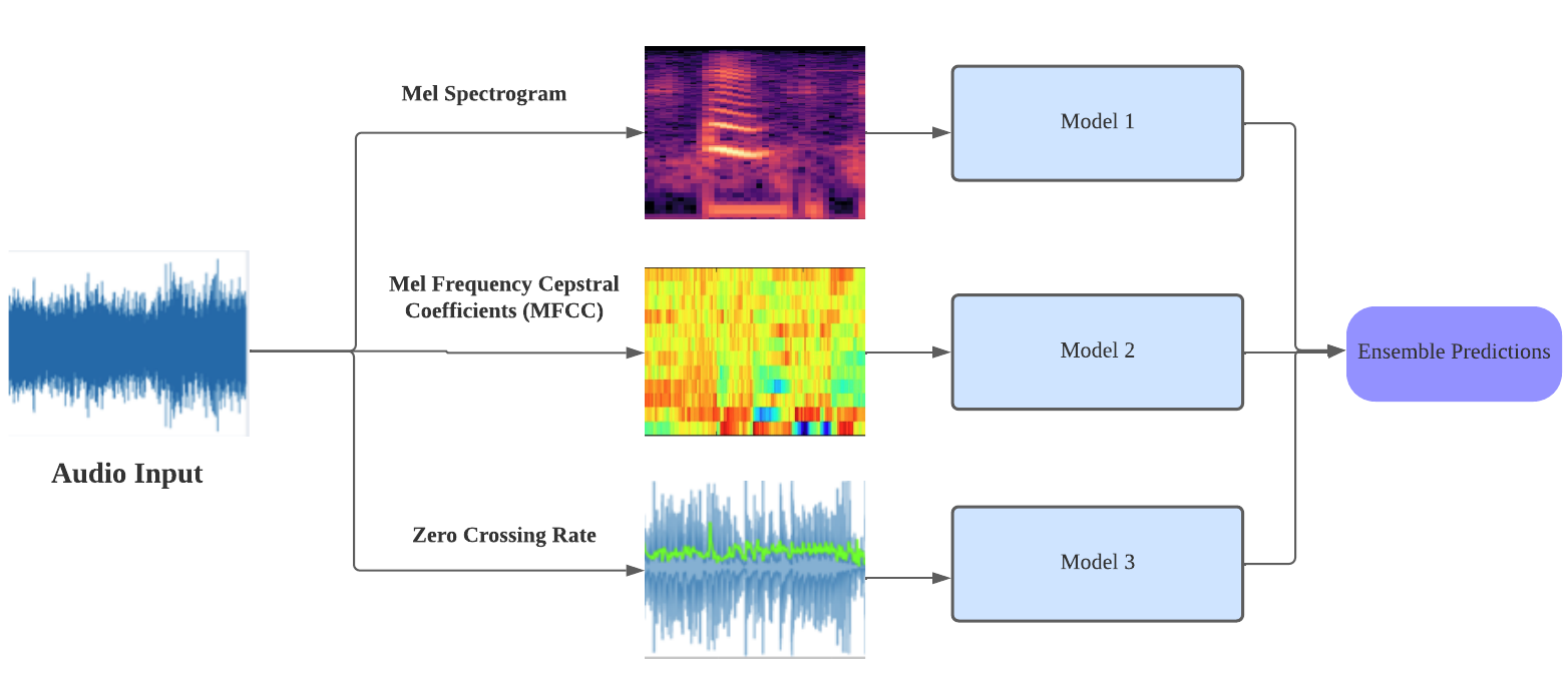
Figure 1: The investigated multi-modality approach with three models

We describe the whole steps during test once models are trained:

• Get probabilities:

  • $P_{MS}$ = $M_{MS}(X_{MS})$

  • $P_{MFCC}$ = $M_{MFCC}(X_{MFCC})$

  • $P_{ZCR}$ = $M_{ZCR}(X_{ZCR})$

• We then explore combination of two feature probabilities first, then we combined all these features probability, like $Average=\frac{P_{MS}+P_{MFCC}+P_{ZCR}}{3}$

• Finally, we predict the class or the label using argmax function:

  • $Predicted_{label}=argmax(Average)$

4 Experiment Design

In this section, we describe our experimental design in three parts: (i) the data set on which we are basing our experiments, (ii) the algorithms we are comparing against, and (iii) the setup of our system and the values defined for the parameters of our algorithms.

4.1 Datasets

We used three different datasets for digit classification in English, Urdu and Gujrati languages. We describe each of the datasets below.

4.1.1 Free Spoken Digits Dataset (FSDD [39])

This dataset is about spoken digits of English pronunciation (0 to 9) and consists of 1500 recordings. These are recorded from 3 different speakers and 50 of each digit per speaker. Each recording is mono and sampled at 8kHz and saved in .wav format. It has 10 classes (0 to 9). All participants are male. Information about audio duration is unknown, but we noticed that its minimum duration length is 1 second and maximum is 2 second.

4.1.2 Audio Urdu Digits Dataset (AUDD [1])

This dataset is an audio spoken digits dataset for Urdu language. This dataset has 25218 samples collected from 740 participants aged between 5 an 89 for diversity purpose, but the majority of participants were 5 to 14 years old and male participants were slightly more numerous than female participants. Each sample is stereo and sampled at 48 $kHz$ and is mono-channel with a minimum length of 1 second and maximum length of 2 seconds. Furthermore, the number of samples in the dataset is almost balanced between all the classes (i.e., digit per age).

4.1.3 Audio Gujarati Digits Dataset (AGDD [5])

This dataset is an audio digits dataset for Gujarati language which has 1940 samples sampled at 44.1 kHz. Recordings are obtained by 20 users, including 14 male and 6 female, from five different regions of Gujarat i.e. Central Zone, North Zone, South Zone, Saurashtra, Kutch Region. Information about duration of audio is unknown but we notice that minimum and maximum duration of audio is 1 and 2 seconds, respectively. Each audio is saved in .wav format.

4.2 Algorithms

We used different deep learning models for generalization purpose. We used 3-layers CNN, EfficientNet [38] and mobileNet [9]. For a fair comparison, we took the same model architectures that were defined in [1, 5]. For the CNN model, we implemented a 3-layer architecture as described in  [1] and shown in Table 1.

Table 1: CNN Model, architecture taken from  [1]

Layer type	Dimensions	Other Details
Input	Input layer	$(32,32,1)$
CNN	$(30,30,64)$	kernel $3\times 3;$ stride 1 ;
		relu activation
Max Pool	$(15,15,64)$	N/A
BN	$(15,15,64)$	default value as
		given in Keras [3]
CNN	$(13,13,64)$	kernel $3\times 3;$ stride 1;
		relu activation
Max Pool	$(6,6,64)$	N/A
BN	$(6,6,64)$	default value as
		given in Keras [3]
CNN	$(4,4,64)$	kernel $3\times 3;$ stride 1;
		relu activation
Max Pool	$(2,2,64)$	N/A
BN	$(2,2,64)$	default value as
		given in Keras [3]
Dropout	$(2,2,64)$	dropout rate=0.1
Flatten	256	N/A
Fully Connected	512	N/A
Dropout	512	dropout rate=0.1
Fully Connected	128	N.A
Dropout	512	dropout rate=0.1
Fully Connected	10	softmax activation

4.3 Setup

Once features are extracted by using MS, MFCC, ZCR, we reshape the features to $32\times 32\times 1$ as 2D images. Each dataset is randomly split into training and test sets with an 8 to 2 ratio. Furthermore, the training set is also split into training and validation sets with a 9 to 1 ratio.

We used hyperparameters as epoch 150, learning rate 0.01, batch size of 64 and set the loss to categorical cross entropy as shown in Equation 2.

$$L(\Theta)=-\sum_{i=1}^{k}y_{i}\log\left(\hat{y}_{i}\right)$$ (2)

where $y_{i}$ is the ground truth, $\hat{y_{i}}$ is the predicted label, $k$ is the number of samples in the batch.

5 Evaluation

We evaluated the performance using accuracy metric (as shown in Equation 3) and time required for testing (in millisecond).

$$A=\frac{P}{T}$$ (3)

where $A$, $P$ and $T$ represent accuracy, correct number of predicted samples and total number of samples, respectively.
We performed each experiment three times and average accuracy is reported. In Tables 2, 3 and 4, the values MS, MFCC and ZCR represent Mel Spectrogram, Mel Frequency Cepstral Coefficients, and Zero Crossing Rate, respectively. In braces, MS means the experiment is performed using a single feature and this is the same for MFCC and ZCR. For two or three features in braces, the model prediction is obtained using an ensemble of models trained using two or three features. EfficientNetB0 to EfficientNetB7 are the different versions of EfficientNet and similarly we used a single version of MobileNetV1.

Tables 2, 3 and 4, also report the average time taken for testing (in milliseconds). We evaluated the testing time for each feature individually and when combined as an ensemble, with each of the considered models and datasets.

Obtained results suggest that testing time is dependent of all dataset, model and feature. For the same dataset, time for CNN with MS is lower than with ZCR. For the same model, time of CNN with MFCC is larger than CNN with MS. For the same feature, time of CNN with MS on AUDD is lower than CNN with MS on FSSD. Otherwise, it is natural that when increasing the number of features, time increases as well. So time for two and three features increases. Overall, obtained results suggest that if we want to achieve a trade-off between accuracy and speed, we should also select our features and models carefully.

For AUDD dataset [1], among single feature experiments, CNN with MS feature achieves the highest performance, whereas the same CNN with the ZCR feature achieves the worst performance. That is due to the loss of sound features during ZCR extraction.

While we are not able to identify a rule on what number of features is ideal during emsembling (i.e., either two or three features at a time), we see that the features showing high performance independently lead to better performance when combined in a feature ensembling. ZCR which achieved less performance acts as a handicap as it drops the performance whenever it is combined with MFCC or MS. MFCC and MS combination with CNN model showed the best performance over previous SOTA performance with an absolute improvement of 3.00%, as shown in Table 2.

Similarly for the FSSD dataset, we performed many experiments using diverse DL models. First we explore single feature based performances. Then, we check combinations of feature ensemblings. Unlike ZCR for AUDD, ZCR for FSSD a shows better performance. Therefore, the combination ZCR with MFCC and MS using either CNN or EfficientNet helps to improve the performance during ensembling and shows superior performance with a 1% improvement to the previous SOTA performance, as shown in Table 3.

Moreover, to check the effectiveness of the approach, we perform the experiment on Audio Gujarati Digits Dataset (AGDD). In AGDD dataset, MS single feature has been effective with CNN and similarly MFCC is also effective. When these two features are used during ensembling, it further improved the performance over SOTA performance with an absolute improvement of 0.2%. However, these two individual features with EfficientNet and MobileNet have shown worse performance than CNN. None of the different DL models using three features ensembling were unable to improve performance due to the presence of the ZCR feature which acted as a handicap–achieving worse performance compared to MS and MFCC features.

Overall, MS and MFCC combination showed the best performance for audio digit classificaiton, nevertheless model selection is very important. MS and MFCC combination with EfficientNet and MobileNet unable to improve the performance. To select the good features, we should also consider the model choice. ZCR with MS and MFCC ensembling is only good choice of selection, whenever it shows good performance individually as shown in Table 2. In the most cases, MS and MFCC has shown the best performance and results suggest that we should use those two features combination for ensembling.

Table 2: Different features accuracy using different models using AUDD [1] dataset

Model Name	Accuracy	Time(ms)
Single feature
Support Vector Machine (MS) [1]	0.65 $\pm$ 0.0	–
Multilayer Perceptron (MS) [1]	0.73 $\pm$ 0.02	–
CNN (MS) [1]	0.86 $\pm$ 0.02	0.264
EfficientNetB0 (MS) [1]	0.84$\pm$ 0.05	1.60
EfficientNetB1 (MS) [1]	0.82$\pm$ 0.02	–
EfficientNetB2 (MS) [1]	0.83$\pm$ 0.04	–
EfficientNetB3 (MS) [1]	0.84$\pm$ 0.06	–
EfficientNetB4 (MS) [1]	0.82$\pm$ 0.03	–
EfficientNetB5 (MS)[1]	0.84$\pm$ 0.04	–
EfficientNetB6 (MS) [1]	0.81$\pm$ 0.06	–
EfficientNetB7 (MS) [1]	0.56$\pm$ 0.07	–
MobileNetV1 (MS)	0.83$\pm$ 0.00	0.531
CNN (MFCC)	0.85 $\pm$ 0.01	0.541
CNN (ZCR)	0.40 $\pm$ 0.03	0.360
EfficientNetB0 (MFCC)	0.81$\pm$ 0.03	1.124
EfficientNetB0 (ZCR)	0.27 $\pm$ 0.02	1.681
MobileNetV1 (MFCC)	0.80$\pm$ 0.02	0.628
MobileNetV1 (ZCR)	0.36 $\pm$ 0.03	0.689
Two Features Ensembler
CNN (MS and MFCC)	0.89 $\pm$ 0.01	0.896
CNN (MS and ZCR)	0.82 $\pm$ 0.03	0.805
CNN (MFCC and ZCR)	0.81 $\pm$ 0.01	0.631
EfficientNetB0 (MS and MFCC )	0.88$\pm$ 0.02	4.431
EfficientNetB0 (MS and ZCR)	0.82$\pm$ 0.03	3.899
EfficientNetB0 (MFCC and ZCR)	0.80$\pm$ 0.02	4.076
MobileNetV1 (MS and MFCC )	0.87$\pm$ 0.03	1.65
MobileNetV1 (MS and ZCR)	0.66$\pm$ 0.02	1.70
MobileNetV1 (MFCC and ZCR)	0.72$\pm$ 0.00	1.13
Three Features Ensembler
CNN (MS, MFCC and ZCR)	0.87 $\pm$ 0.03	0.8167
EfficientNetB0 (MS, MFCC and ZCR)	0.86$\pm$ 0.03	5.859
MobileNetV1 (MS, MFCC and ZCR)	0.85$\pm$ 0.05	2.540

Table 3: Performance comparison multiple features using different models on FSSD [39]

Model Name	Accuracy	Time(ms)
CNNDigitReco-speakerindependent [36]	0.78 $\pm$ 0.0	–
Single Feature
Support Vector Machine [41]	0.90 $\pm$ 0.02	–
Random Forest [41]	0.96 $\pm$ 0.06	–
English Digit Model[21]	0.97 $\pm$ 0.09	–
CNN (MS) [1]	0.973 $\pm$ 0.01	0.3441
CNN (MFCC)	0.978 $\pm$ 0.03	0.2895
CNN (ZCR)	0.572 $\pm$ 0.08	0.306
EfficientNetB0 (MS)	0.947 $\pm$ 0.05	1.154
EfficientNetB0 (MFCC)	0.968 $\pm$ 0.07	0.740
EfficientNetB0 (ZCR)	0.378 $\pm$ 0.06	1.148
MobileNetV1 (MS)	0.877 $\pm$ 0.01	4.855
MobileNetV1 (MFCC)	0.980 $\pm$ 0.02	3.367
MobileNetV1 (ZCR)	0.538 $\pm$ 0.03	4.035
Two Feature Ensembler
CNN (MS and MFCC)	0.987 $\pm$ 0.02	0.651
CNN (MS and ZCR)	0.980 $\pm$ 0.03	0.630
CNN (MFCC and ZCR)	0.977 $\pm$ 0.05	0.639
EfficientNetB0 (MS and MFCC)	0.987 $\pm$ 0.07	2.811
EfficientNetB0 (MS and ZCR)	0.957 $\pm$ 0.08	3.583
EfficientNetB0 (MFCC and ZCR)	0.970 $\pm$ 0.01	2.838
MobileNetV1 (MS and MFCC)	0.985 $\pm$ 0.05	4.9
MobileNetV1 (MS and ZCR)	0.960 $\pm$ 0.06	1.682
MobileNetV1 (MFCC and ZCR)	0.970 $\pm$ 0.09	2.308
Three Features Ensembler
CNN (MS, MFCC, ZCR)	0.99 $\pm$ 0.03	0.921
EfficientNetB0 (MS, MFCC, ZCR)	0.99 $\pm$ 0.04	4.977
MobileNetV1 (MS, MFCC, ZCR)	0.987 $\pm$ 0.05	2.903

Table 4: Performance comparison multiple features using different models on Gujarati Digits dataset[5]

Model Name	Accuracy	Time(ms)
Single Feature
Gujarati Digits Model[5]	0.75 $\pm$ 0.02	–
CNN (MS) [1]	0.970 $\pm$ 0.03	1.770
CNN (MFCC)	0.959 $\pm$ 0.05	1.761
CNN (ZCR)	0.572 $\pm$ 0.07	1.750
EfficientNetB0 (MS)	0.880 $\pm$ 0.02	9.402
EfficientNetB0 (MFCC)	0.907 $\pm$ 0.01	9.781
EfficientNetB0 (ZCR)	0.321 $\pm$ 0.04	9.536
MobileNetV1 (MS)	0.856 $\pm$ 0.01	0.63
MobileNetV1 (MFCC)	0.89 $\pm$ 0.05	0.791
MobileNetV1 (ZCR)	0.557 $\pm$ 0.03	1.35
Two Features Ensembler
CNN (MS and MFCC)	0.972 $\pm$ 0.04	2.996
CNN (MS and ZCR)	0.936 $\pm$ 0.08	1.006
CNN (MFCC and ZCR)	0.943 $\pm$ 0.07	1.723
EfficientNetB0 (MS and MFCC)	0.970 $\pm$ 0.01	3.491
EfficientNetB0 (MS and ZCR)	0.881 $\pm$ 0.06	3.338
EfficientNetB0 (MFCC and ZCR)	0.94 $\pm$ 0.01	3.334
MobileNetV1 (MS and MFCC)	0.933 $\pm$ 0.03	1.84
MobileNetV1 (MS and ZCR)	0.80 $\pm$ 0.04	2.396
MobileNetV1 (MFCC and ZCR)	0.884 $\pm$ 0.02	2.280
Three Features Ensembler
CNN (MS, MFCC and ZCR)	0.966 $\pm$ 0.03	1.254
EfficientNetB0 (MS, MFCC and ZCR)	0.948 $\pm$ 0.05	5.261
MobileNetV1 (MS, MFCC and ZCR)	0.917 $\pm$ 0.03	3.520

We have also analyzed the stability of the models with a single feature at a time and their behavior during validation on AUDD, FSSD, and AGDD respectively, as shown in Figures 2.

Interestingly, all Figures 2 have the same pattern as CNN with the MS feature, i.e., they are very stable. Furthermore, the analysis shows consistent accuracy improvements from one epoch to another, except for EfficientNet with ZCR which has shown a worse performance. Feature-wise, MS and MFCC are nearly equally successful among all cases with the different models, whereas the use of ZCR drops the performance of all models.

Overall, Figures 2 suggest that to achieve the best performance and stability, the choice of model is important, whereas MS seems to be an excellent feature extractor and the feature of choice.

In summary, we have shown that ensembling all features at the same time does not guarantee achieving the best performance (in the contrary, it acts as a handicap) and that beyond the selection of features, the choice of the model is important. Therefore, it will be beneficial to design automatic and interpretable ensembling techniques, potentially through reinforcement learning techniques such as grammar-guided genetic programming [16, 34, 31, 30, 32]. Furthermore, while we have only focused on accuracy in this work, it is possible that a feature/model ensembling does not achieve the best accuracy, but performs better on other metrics. Therefore, it will be beneficial to formulate the problem as a multi-objective feature selection [29, 27, 28, 33].

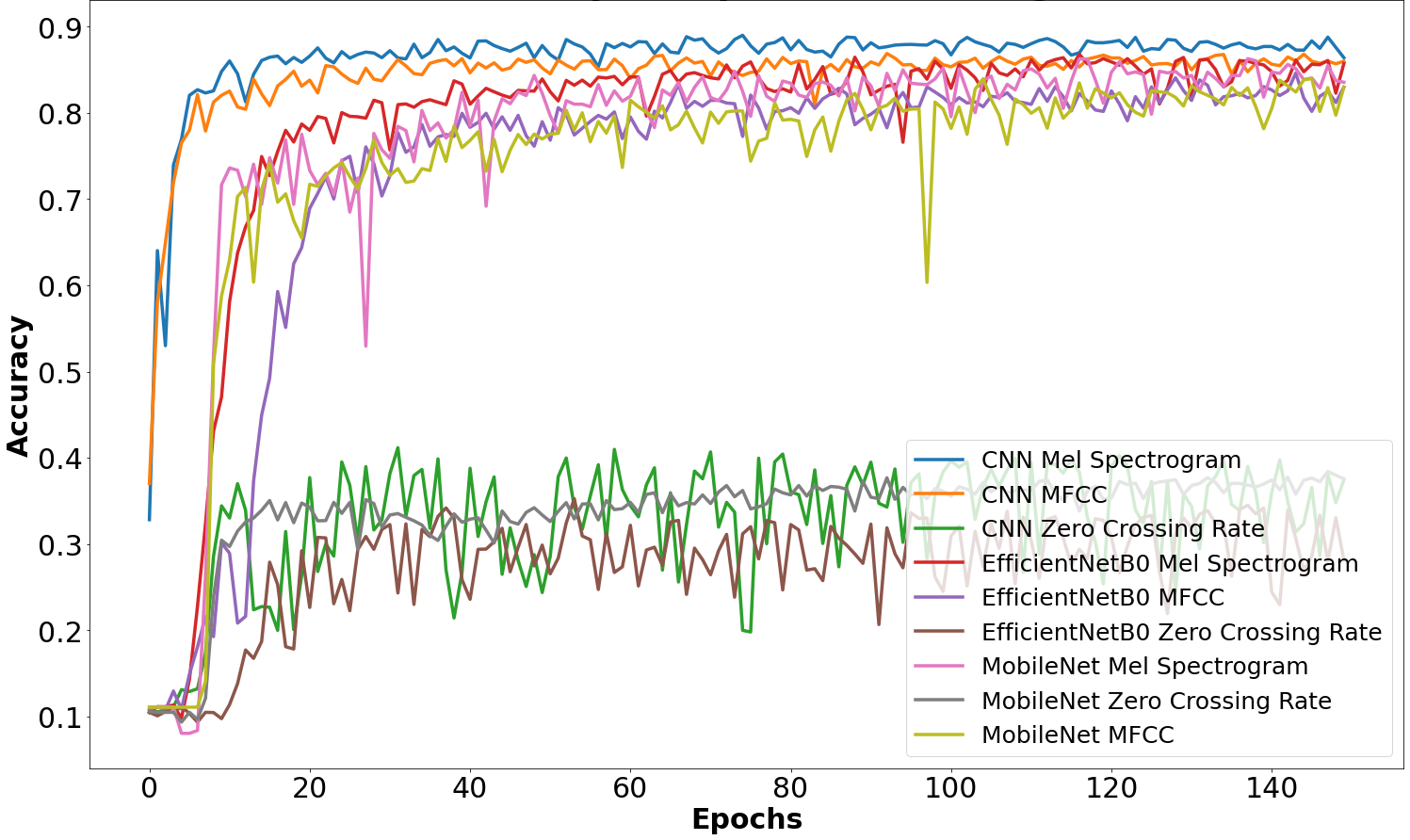
(a) Urdu digits Dataset

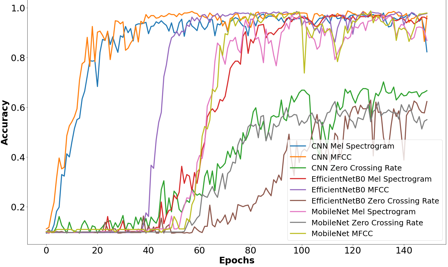
(b) FSDD Dataset

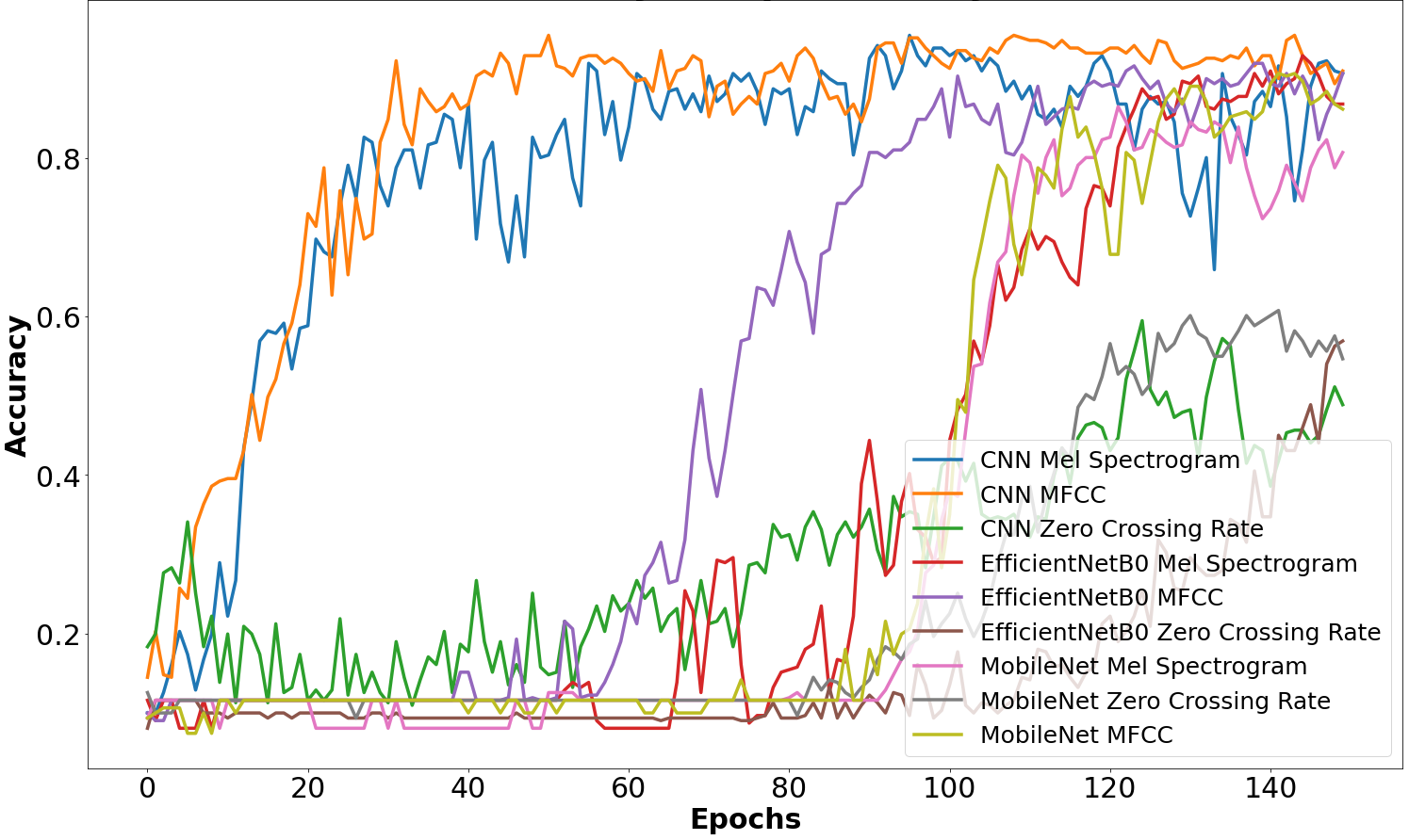
(c) Gujarati Dataset

Figure 2: Validation Accuracy over Epochs on the Different Datasets

6 Conclusion

This paper investigates the use of multi-feature ensemblers, combining three state-of-the-art audio features (i.e., Mel Spectrogram, Mel Frequency Cepstral Coefficients, and Zero Crossing Rate) to alleviate the performance constrained by the features when dealing with audio classification tasks.

In our work, we sought to explore different combinations of the three state-of-the-arts features with a diverse set of models, on different datasets with the goal of identifying the best combination of features and models. To check the generalization of our results, we used three different audio datasets including, Free Spoken Digits Dataset, Audio Urdu Digits Dataset and Audio Gujarati Digits Dataset.

We trained our models with each feature individually, then with a combination of two and three features. We evaluated the performance of each configuration, i.e., model and feature(s) in terms of accuracy and testing time. Our thorough experimental evaluation has shown that it is only better to combine features that already perform well individually (i.e., mostly Mel Spectrogram, Mel Frequency Cepstral Coefficients).

Our future research direction is in two folds: (i) to reduce testing time by stacking multiple features and (ii) to explore these features from data augmentation perspective to generate novel features.

7 Acknowledgment

This research was supported by Science Foundation Ireland (SFI) under grant numbers 18/CRT/6223, 13/RC/2094$\_$P2 (Lero SFI Centre for Software) and 13/RC/2106$\_$P2 (ADAPT SFI Research Centre for AI-Driven Digital Content Technology).

Authors

	Muhammad Turab is an undergraduate student at MUET, Jamshoro. He has been working in the field of Deep Learning and Machine learning for two years. He has completed more than 70 projects on GitHub. His research interests include deep learning, computer vision and data augmentation for medical imaging.
	Teerath Kumar received his Bachelor’s degree in Computer Science with distinction from National University of Computer and Emerging Science (NUCES), Islamabad, Pakistan, in 2018. Currently, he is pursuing PhD from Dublin City University, Ireland. His research interests include advanced data augmentation, deep learning for medical imaging, generative adversarial networks and semi-supervised learning.
	Malika Bendechache is a Lecturer/Assistant Professor in the School of Computing at Dublin City University, Ireland, and a Funded Investigator at both ADAPT and Lero Science Foundation Ireland research centres. Malika holds a PhD in Computer Science from University College Dublin, Ireland. Her research interests span the areas of Big data Analytics, Machine Learning, Data Governance, Parallel and Distributed Systems, Cloud/Edge/Fog Computing, Blockchain, Security, and Privacy.
	Takfarinas Saber is a Lecturer/Assistant Professor in the School of Computer Science at National University of Ireland, Galway, Ireland, and a Funded-Investigator in Lero, the Science Foundation Ireland Research Centre for Software. Takfarinas holds a PhD in Computer Science from University College Dublin, Ireland. His area of expertise is in the optimisation of Complex Software Systems such as Cloud Computing, Smart Cities, Distributed Systems, and Wireless Communication Networks.

References

- [1] Aisha Aiman, Yao Shen, Malika Bendechache, Irum Inayat, and Teerath Kumar. Audd: Audio urdu digits dataset for automatic audio urdu digit recognition. Applied Sciences, 11(19):8842, 2021.
- [2] David Warren Ball. Field guide to spectroscopy, volume 8. Spie Press Bellingham, Washington, 2006.
- [3] F. & Others Chollet. Keras. 2015.
- [4] Hilmi Egemen Ciritoglu, Takfarinas Saber, Teodora Sandra Buda, John Murphy, and Christina Thorpe. Towards a better replica management for hadoop distributed file system. In 2018 IEEE International Congress on Big Data (BigData Congress), pages 104–111. IEEE, 2018.
- [5] Nikunj Dalsaniya, Sapan H Mankad, Sanjay Garg, and Dhuri Shrivastava. Development of a novel database in gujarati language for spoken digits classification. In International Symposium on Signal Processing and Intelligent Recognition Systems, pages 208–219. Springer, 2019.
- [6] Liang Gao, Kele Xu, Huaimin Wang, and Yuxing Peng. Multi-representation knowledge distillation for audio classification. Multimedia Tools and Applications, pages 1–24, 2022.
- [7] Theodoros Giannakopoulos and Aggelos Pikrakis. Introduction to audio analysis: a MATLAB® approach. Academic Press, 2014.
- [8] Shawn Hershey, Sourish Chaudhuri, Daniel P. W. Ellis, Jort F. Gemmeke, Aren Jansen, R. Channing Moore, Manoj Plakal, Devin Platt, Rif A. Saurous, Bryan Seybold, Malcolm Slaney, Ron J. Weiss, and Kevin Wilson. Cnn architectures for large-scale audio classification. In 2017 IEEE International Conference on Acoustics, Speech and Signal Processing (ICASSP), pages 131–135, 2017.
- [9] Andrew G Howard, Menglong Zhu, Bo Chen, Dmitry Kalenichenko, Weijun Wang, Tobias Weyand, Marco Andreetto, and Hartwig Adam. Mobilenets: Efficient convolutional neural networks for mobile vision applications. arXiv preprint arXiv:1704.04861, 2017.
- [10] Chadawan Ittichaichareon, Siwat Suksri, and Thaweesak Yingthawornsuk. Speech recognition using mfcc. In International conference on computer graphics, simulation and modeling, volume 9, 2012.
- [11] Niranjan K, Shankar Kumar S, and Vedanth S. Ensemble and multi model approach to environmental sound classification. In 2021 Fourth International Conference on Electrical, Computer and Communication Technologies (ICECCT), pages 1–5, 2021.
- [12] Jongpil Lee, Jiyoung Park, Keunhyoung Luke Kim, and Juhan Nam. Sample-level deep convolutional neural networks for music auto-tagging using raw waveforms. arXiv preprint arXiv:1703.01789, 2017.
- [13] Xinyu Li, Venkata Chebiyyam, and Katrin Kirchhoff. Multi-stream network with temporal attention for environmental sound classification. arXiv preprint arXiv:1901.08608, 2019.
- [14] Beth Logan. Mel frequency cepstral coefficients for music modeling. In In International Symposium on Music Information Retrieval. Citeseer, 2000.
- [15] Guojun Lu and Templar Hankinson. An investigation of automatic audio classification and segmentation. In WCC 2000-ICSP 2000. 2000 5th International Conference on Signal Processing Proceedings. 16th World Computer Congress 2000, volume 2, pages 776–781. IEEE, 2000.
- [16] David Lynch, Takfarinas Saber, Stepán Kucera, Holger Claussen, and Michael O’Neill. Evolutionary learning of link allocation algorithms for 5g heterogeneous wireless communications networks. In Proceedings of the Genetic and Evolutionary Computation Conference, pages 1258–1265, 2019.
- [17] Sayf A Majeed, Hafizah Husain, Salina Abdul Samad, and Tariq F Idbeaa. Mel frequency cepstral coefficients (mfcc) feature extraction enhancement in the application of speech recognition: a comparison study. Journal of Theoretical and Applied Information Technology, 79(1):38, 2015.
- [18] Martin McKinney and Jeroen Breebaart. Features for audio and music classification. 2003.
- [19] Loris Nanni, Yandre MG Costa, Diego Rafael Lucio, Carlos Nascimento Silla Jr, and Sheryl Brahnam. Combining visual and acoustic features for audio classification tasks. Pattern Recognition Letters, 88:49–56, 2017.
- [20] Loris Nanni, Gianluca Maguolo, Sheryl Brahnam, and Michelangelo Paci. An ensemble of convolutional neural networks for audio classification. Applied Sciences, 11(13):5796, 2021.
- [21] Seham Nasr, Muhannad Quwaider, and Rizwan Qureshi. Text-independent speaker recognition using deep neural networks. In 2021 International Conference on Information Technology (ICIT), pages 517–521. IEEE, 2021.
- [22] Jayashree Padmanabhan and Melvin Jose Johnson Premkumar. Machine learning in automatic speech recognition: A survey. IETE Technical Review, 32(4):240–251, 2015.
- [23] Kamalesh Palanisamy, Dipika Singhania, and Angela Yao. Rethinking cnn models for audio classification. arXiv preprint arXiv:2007.11154, 2020.
- [24] Daniel S Park, William Chan, Yu Zhang, Chung-Cheng Chiu, Barret Zoph, Ekin D Cubuk, and Quoc V Le. Specaugment: A simple data augmentation method for automatic speech recognition. arXiv preprint arXiv:1904.08779, 2019.
- [25] Karol J Piczak. Environmental sound classification with convolutional neural networks. In 2015 IEEE 25th international workshop on machine learning for signal processing (MLSP), pages 1–6. IEEE, 2015.
- [26] Karol J Piczak. Esc: Dataset for environmental sound classification. In Proceedings of the 23rd ACM international conference on Multimedia, pages 1015–1018, 2015.
- [27] Takfarinas Saber, Malika Bendechache, and Anthony Ventresque. Incorporating user preferences in multi-objective feature selection in software product lines using multi-criteria decision analysis. In International Conference on Optimization and Learning, pages 361–373. Springer, 2021.
- [28] Takfarinas Saber, David Brevet, Goetz Botterweck, and Anthony Ventresque. Is seeding a good strategy in multi-objective feature selection when feature models evolve? Information and Software Technology, 95:266–280, 2018.
- [29] Takfarinas Saber, David Brevet, Goetz Botterweck, and Anthony Ventresque. Reparation in evolutionary algorithms for multi-objective feature selection in large software product lines. SN Computer Science, 2(3):1–14, 2021.
- [30] Takfarinas Saber, David Fagan, David Lynch, Stepan Kucera, Holger Claussen, and Michael O’Neill. A hierarchical approach to grammar-guided genetic programming the case of scheduling in heterogeneous networks. In TPNC, pages 118–134, 2018.
- [31] Takfarinas Saber, David Fagan, David Lynch, Stepan Kucera, Holger Claussen, and Michael O’Neill. Hierarchical grammar-guided genetic programming techniques for scheduling in heterogeneous networks. In CEC, 2020.
- [32] Takfarinas Saber, David Fagan, David Lynch, Stepan Kucera, Holger Claussen, and Michael O’Neill. A multi-level grammar approach to grammar-guided genetic programming: the case of scheduling in heterogeneous networks. GPEM, pages 1–39, 2019.
- [33] Takfarinas Saber, James Thorburn, Liam Murphy, and Anthony Ventresque. VM reassignment in hybrid clouds for large decentralised companies: A multi-objective challenge. Future Generation Computer Systems, 79:751–764, 2018.
- [34] Takfarinas Saber and Shen Wang. Evolving better rerouting surrogate travel costs with grammar-guided genetic programming. In IEEE CEC, pages 1–8, 2020.
- [35] Yuma Sakashita and Masaki Aono. Acoustic scene classification by ensemble of spectrograms based on adaptive temporal divisions. Detection and Classification of Acoustic Scenes and Events (DCASE) Challenge, 2018.
- [36] Oscar Saz. CNNDigitReco-speakerindependent. https://www.kaggle.com/saztorralba/cnndigitreco-speakerindependent, 2020.
- [37] Alexander Schindler, Thomas Lidy, and Andreas Rauber. Multi-temporal resolution convolutional neural networks for acoustic scene classification. arXiv preprint arXiv:1811.04419, 2018.
- [38] Mingxing Tan and Quoc Le. Efficientnet: Rethinking model scaling for convolutional neural networks. In International conference on machine learning, pages 6105–6114. PMLR, 2019.
- [39] Zohar Jackson; Cesar Souza; Jason Flaks; Yuxin Pan; Hereman Nicolas; Adhish Thite. A free audio dataset of spoken digits. think mnist for audio. https://doi.org/10.5281/zenodo.1342401, 2018. [Online; accessed 1-March-2022].
- [40] BZJLS Thornton. Audio recognition using mel spectrograms and convolution neural networks. 2019.
- [41] Inam Ur Rehman. Classification on fsdd using spectograms. https://www.kaggle.com/iinaam/classification-on-fsdd-using-spectograms, 2021.
- [42] Qi Wang, Xiang He, and Xuelong Li. Locality and structure regularized low rank representation for hyperspectral image classification. IEEE Transactions on Geoscience and Remote Sensing, 57(2):911–923, 2018.
- [43] Yong Xu, Qiuqiang Kong, Wenwu Wang, and Mark D Plumbley. Large-scale weakly supervised audio classification using gated convolutional neural network. In 2018 IEEE international conference on acoustics, speech and signal processing (ICASSP), pages 121–125. IEEE, 2018.
- [44] Shiqing Zhang, Shiliang Zhang, Tiejun Huang, and Wen Gao. Speech emotion recognition using deep convolutional neural network and discriminant temporal pyramid matching. IEEE Transactions on Multimedia, 20(6):1576–1590, 2017.