Mandheling: Mixed-Precision On-Device DNN Training with DSP Offloading

Abstract.

This paper proposes Mandheling, the first system that enables highly resource-efficient on-device training by orchestrating the mixed-precision training with on-chip Digital Signal Processing (DSP) offloading. Mandheling fully explores the advantages of DSP in integer-based numerical calculation by four novel techniques: (1) a CPU-DSP co-scheduling scheme to mitigate the overhead from DSP-unfriendly operators; (2) a self-adaptive rescaling algorithm to reduce the overhead of dynamic rescaling in backward propagation; (3) a batch-splitting algorithm to improve the DSP cache efficiency; (4) a DSP-compute subgraph reusing mechanism to eliminate the preparation overhead on DSP. We have fully implemented Mandheling and demonstrate its effectiveness through extensive experiments. The results show that, compared to the state-of-the-art DNN engines from TFLite and MNN, Mandheling reduces the per-batch training time by 5.5$\times$ and the energy consumption by 8.9$\times$ on average. In end-to-end training tasks, Mandheling reduces up to 10.7$\times$ convergence time and 13.1$\times$ energy consumption, with only 1.9%–2.7% accuracy loss compared to the FP32 precision setting.

1. Introduction

With the ever-increasing concerns of privacy (gdpr, ), empowering a mobile device to train a deep neural network (DNN) locally, i.e., on-device training is recently attracting attentions from both academia and industry (deeptype, ; siri-fl, ; gboard-fl, ). Without giving away the training data, on-device training enables (i) geo-distributed devices to collaboratively establish a high-accuracy model (hard2018federated, ; bonawitz2019towards, ) or (ii) a single device to personalize and adapt its model to its own environments (deeptype, ).

However, a key obstacle towards practical on-device training is its huge resource cost. According to our preliminary measurements with two popular DL libraries (TFLite (tflite, ) and MNN (mnn, )), training ResNet-50 with one batch (batch size 32) takes 4.6 GB memory and 36.4 seconds on the smartphone XiaoMI 10 equipped with Snapdragon 865 CPU. The consumed energy equals to watching a 1080P-definition video for 111.2 seconds. In an end-to-end learning scenario, it typically takes thousands or even more such batches of training and the accumulated cost becomes prohibitively expensive. Unfortunately, this issue has not been well explored by the research community. Existing studies gaining impressive benefits for on-device inference tasks (wang2021asymo, ; chen2018tvm, ; liu2019optimizing, ; huynh2017deepmon, ; xu2018deepcache, ) can be hardly applied to on-device training due to the huge gap between inference and training workloads, e.g., the different computation patterns and accuracy requirements.

To optimize the performance of on-device training, this work is motivated by two key observations. First, traditional DNN training mostly performs on FP32 data format to achieve good model accuracy. However, the ML community has recently proposed various mixed-precision training algorithms (wang2020niti, ; zhou2021octo, ; wu2016binarized, ; lin2015neural, ; rastegari2016xnor, ; zhou2018adaptive, ; lin2017towards, ; courbariaux2015binaryconnect, ; jacob2018quantization, ; zhang2020fixed, ; yang2020training, ; zhong2020towards, ), where the weights and activations generated during training are represented not only by FP32 but also by lower-precision formats such as INT8 and INT16. By exploiting the hardware features in accelerating integer operations, these algorithms have been demonstrated to be effective in reducing the training-time resource cost while guaranteeing the convergence accuracy, i.e., only 1.3% loss on CIFAR-10 (yang2020training, ). Second, modern mobile SoCs often consist of heterogeneous processors, among which the Digital Signal Processor (DSP) is ubiquitously available and particularly suits integer operations, i.e., INT8-based matrix multiplication. For example, Hexagon 698 DSP (QualcommHexagon, ) is adequate to execute 128 INT8 operations in one cycle and has been demonstrated to be 11.3$\times$/4.0$\times$ more energy-efficient than CPU/GPU in DL inference tasks (zhang2022comprehensive, ), respectively. Intuitively, under the mixed-precision training setting, we are interested in a question whether we can partially offload the training workloads, especially those integer-based operations, from CPU to DSP to reduce the cost of on-device training.

In this paper, we propose a first-of-its-kind system, namely Mandheling, which enables highly resource-efficient, mixed-precision on-device training with on-chip DSP offloading. To facilitate developers in using different types of training algorithms on Mandheling, we investigate popular mixed-precision training algorithms and extract the key principles from them. Based on those principles, we incorporate a unified abstraction into Mandheling as will be discussed in $\S$3.2. With a given training algorithm and the model to be trained, Mandheling aims to minimize the training cost by judiciously co-scheduling various training operators to mobile DSP (mostly) and CPU. When designing Mandheling, however, we need to address the following major challenges that have not been explored in prior literature.

• Dealing with DSP-unfriendly operators. In a typical mixed-precision training algorithm, some operators like Transpose and Normalization run slowly on DSP due to their irregular memory accesses (mittal2016survey, ) or lack of architecture-level support on DSP. A judicious scheme to determine what operators to be offloaded to DSP while others are placed on CPU is needed to fully exploit those heterogeneous processors.

• Dynamic rescaling does not fit DSP. During the training, dynamic rescaling (wang2020niti, ; zhang2020fixed, ; yang2020training, ; zhong2020towards, ) is a critical operation to quantize/dequantize among different data types. We observe that this operation runs slowly on DSP and can easily compromise the benefits of using DSP. Because dynamic scaling is inserted into each layer with the low-precision data type, simply scheduling it to CPU like other DSP-unfriendly operators incurs high context switching overhead, therefore needs to be optimized exclusively.

• Exhausted data cache. Training workloads impose high pressure on the DSP cache and a vanilla implementation leads to a low cache hit ratio. The reasons are twofold. First, training tasks often require a large batch size, which results in frequent memory accesses for accessing intermediate data. Second, the DSP cache is often smaller than the CPU cache, e.g., only half for L2 cache on Snapdragon 865. Considering that fully utilizing the processor cache is a killing factor towards memory-intensive operations such as convolution weight gradients (wang2021asymo, ), exhausted data cache on DSP is likely to act as the bottleneck in the training process.

• Costly compute graph preparation. Unlike inference tasks, on-device training tasks usually use dynamic graphs to facilitate developers in development and debugging (pytorch, ). However, preparing the compute graph on DSP takes a considerable amount of time for allocating DSP memory, building graph-to-operation reference, etc. Therefore, how to eliminate the compute graph preparation under a tight memory budget of DSP is critical to Mandheling.

Key techniques of Mandheling. To address the preceding challenges, Mandheling presents the following novel techniques to fully unleash the DSP computing capacity:

• CPU-DSP co-scheduling ($\S$3.3) is proposed to mitigate the overhead of DSP-unfriendly operators. The key idea is to reduce the number of context switchings brought by DSP-unfriendly operators and overlap the CPU and DSP execution as much as possible. This is achieved through our novel scheduling algorithm that considers the latency of the operator executing on different processors and the overhead of CPU-DSP context switching.

• Self-adaptive rescaling ($\S$3.4) is proposed to significantly reduce the overhead of dynamic rescaling by adaptively lowering its invoking frequency. This is motivated by our micro-experiments which demonstrate that, after the early stage of training, the actual changing frequency of the scale factor becomes low and its value becomes fairly stable.

• Batch splitting ($\S$3.5) is proposed to reduce the cache pressure on DSP and so as to increase the cache hit ratio. Mandheling runs the intra-operator partition at the batch dimension because this solution does not influence the inputs and weights of the original convolution operation, thus causing no redundant computations. Mandheling uses an intuitive yet effective method to identify the splitting point of batch size. It also provides an integer-only scheme to efficiently concatenate the output from the split batch.

• DSP-compute subgraph reuse ($\S$3.6) is proposed to eliminate the preparation overhead of DSP compute graph. This is motivated by a key observation that the model structure is rarely changed during the training phase. To further tackle the memory constraint of DSP, we provide a practical subgraph-reusing algorithm based on the minimum dynamic memory allocation/deallocation principle.

Implementation and evaluation We have fully implemented Mandheling with 15k LoC in C/C++ and 800 LoC in assembly language. Mandheling is a standalone framework that supports models exported from different front-end frameworks, e.g., TensorFlow (tensorflow, ) and PyTorch (pytorch, ) and is compatible with various mixed-precision training algorithms. We then conducted extensive experiments on 6 typical DNN models (VGG-11/16/19 (simonyan2014very, ), ResNet-18/34 (he2016deep, ), and InceptionV3 (szegedy2016rethinking, )) and 3 commodity mobile devices (XiaoMI 11 Pro, XiaoMI 10, and Redmi Note9 Pro). The results demonstrated that, compared to native supports from TFLite and MNN, Mandheling can reduce the per-batch training time and energy consumption by 5.5$/$8.9$\times$ on average and up to 8.3$\times$/12.5$\times$, respectively. Furthermore, compared to GPU-enhanced training, Mandheling speeds up the per-batch training time by 7.1$\times$ and reduces the energy consumption by 5.8$\times$ on average. In an end-to-end training on a single device, compared with FP32-based training algorithm and MNN, Mandheling accelerates the model convergence by 5.7$\times$ on average and reduces the total energy consumption by 7.8$\times$ on average. The improvements are even more profound in a federated learning scenario with 8.0$\times$ convergence speedup and 10.6$\times$ energy reduction on average. Meanwhile, the accuracy of trained models drops marginally with only 1.9%-2.7% loss compared to the accuracy of FP32 precision setting, which is consistent with the theoretical results adopted by the ML community (wang2020niti, ; zhou2021octo, ; wu2016binarized, ; lin2015neural, ; rastegari2016xnor, ; zhou2018adaptive, ; lin2017towards, ; courbariaux2015binaryconnect, ; jacob2018quantization, ; zhou2016dorefa, ). The ablation study further distinguishes the effectiveness of every single key technique of Mandheling.

Contributions are summarized as following.

• We thoroughly explore the opportunities and challenges of DSP offloading for mixed-precision on-device training.

• We design and implement the first DSP-offloading based mixed-precision on-device training framework, which incorporates four novel techniques, i.e., self-adaptive rescaling, batch splitting, CPU-DSP co-scheduling, and DSP compute subgraph resue. The system will be fully open-sourced soon on Github.

• We evaluate Mandheling with representative DNN models and commodity mobile devices. The results demonstrate Mandheling’s superior effectiveness and practical value.

2. Background and Motvations

We briefly introduce some background and our motivations.

2.1. On-Device DNN Training

A trend to deploy DNN training on devices locally is emerging, especially with the data privacy concerns (like GDPR (gdpr, )) in AI applications. Similar to DNN training on the cloud/server, the on-device training also conducts mini-batch sampling strategy, where each batch’s training comprises of three stages: the forward pass, the backward pass, and the weight update. The forward pass loads inputs and calculates the loss; the backward pass usually employs a specific optimizer like Stochastic Gradient Descent (SGD) (bottou2010large, ) to obtain the gradients; lastly, the gradients are applied to the weights for model update. Compared to the on-device inference, the training task is more resource-consuming because: (i) the backward pass contains about 2$\times$ FLOPs as forward pass (the same as inference); (ii) a training process often involves hundreds or even thousands of mini-batches.

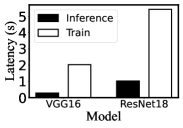
(a) Comparison of inference and training time (batch size = 64.)

(b) Power consumption of different Apps and DNN training on devices.

Figure 1. Preliminary measurements that highlight the huge resource cost of on-device training.

We conducted two measurement studies to highlight the prohibitively high resource cost of on-device training. Figure 1(a) shows that the DNN training takes 7.14$\times$ more time than inference with the same batch size, which is larger than the theoretical FLOPs gap (about 3$\times$). That is because training ops, especially for weight gradient ops, are more difficult to optimize because of the dynamic input width and height of the feature map. Besides, Figure 1(b) shows that on-device training consumes more energy than typical video players (TikTok (tiktok, ), YouTube (youtube, )) and gaming apps (Genshin Impact (genshin, )). For instance, training one batch (BS=32) of the ResNet-50 model costs the same energy as watching 36.4 seconds of videos on YouTube. Considering the minimal granularity for training is usually one epoch which, let’s say, contains 1,000 mini-batches, the energy cost is as high as watching 7.91 hours of videos on YouTube.

2.2. Mixed-Precision Training

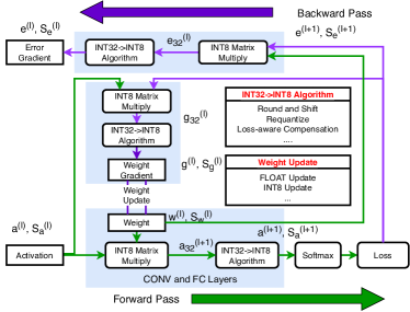
Figure 2. Workflow of mixed-precision training.

To reduce the resource cost of DNN training, mixed-precision training algorithms have been proposed (wang2020niti, ; zhou2021octo, ; wu2016binarized, ; lin2015neural, ; rastegari2016xnor, ; zhou2018adaptive, ; lin2017towards, ; courbariaux2015binaryconnect, ; jacob2018quantization, ; zhou2016dorefa, ). These algorithms mainly exploit the feature that the data in DNNs (including the activation, weights, bias, and gradients) are usually in high redundancy (louizos2018relaxed, ), therefore their representation precision can be reduced, e.g., from FP32 to FP16/INT8. Fewer bits per number benefits the DNN training to run faster through the single-instruction-multiple-data (SIMD) hardware parallelism, which is commonly available on mobile processors (wang2021comprehensive, ). Here, we use INT8 training as an example to illustrate how typical mixed-precision training algorithms work. Figure 2 shows an exemplified workflow.

Forward pass. After quantization, activation $a^{(l)}$ and weight $w^{(l)}$ are INT8 numbers with scale factors $S_{a}^{(l)}$ and $S_{w}^{(l)}$. With INT8 matrix multiply which is used to replace traditionally FP32-based multiplication, we can obtain intermediate INT32 activation $a_{32}^{(l+1)}$. To transform the intermediate results to INT8 numbers, an INT32-to-INT8 algorithm is needed, such as Round and Shift (wang2020niti, ), Loss-aware Compensation (zhou2021octo, ), or Requantize (tensorflow, ). When forwarding to the final layer, the activations are input to the softmax and loss layer.

Backward pass and weight update. The obtained INT8 error gradients $e^{(l+1)}$ will multiply with $w^{(l)}$ and $a^{(l)}$ to obtain intermediate INT32 error gradients $e_{32}^{(l)}$ and weight gradients $g_{32}^{(l)}$. Also through the INT32 to INT8 algorithm, we can get the error and weight gradients of the l-th layer $e^{(l)}$ and $g^{(l)}$ with their scale factor $S_{e}^{(l)}$ and $S_{g}^{(l)}$. Finally, the model weights are updated by gradient $g^{(l)}$ with the global learning rate and other hyperparameters. The update method can be divided into two categories: FLOAT update and INT8 update, which means the former one can support changing scale factor.

2.3. Mobile DSP Offloading

DSP (Digital Signal Processor) is originally designed for processing digital signals like audio with high energy efficiency. Almost each mobile SoC includes DSP, where the most common is Hexagon produced by Qualcomm (QualcommHexagon, ). In 2016 Qualcomm announced Hexagon 680 DSP – the first DSP with Hexagon Vector Extensions (HVX) designed to allow significant compute workloads for advanced imaging, and computer vision (dsp-processor, ). Given its popularity, this work targets Hexagon DSP to run the DNN training workloads, but its techniques are compatible with other DSP hardware as well.

Hexagon DSP architecture. Nowaday Hexagon DSP contains hexagon cores and a SIMD coprocessor. The former one performs general-purpose processing while the latter one is good at vector computation (hexagon-dsp-sdk, ). Mandheling mainly exploits the SIMD co-processor which can process 1024-bit fixed point data inside one HVX instruction, or 128 INT8 mathematical functions like add and multiply in one cycle. Besides, the hexagon core’s clock frequency is 500 MHz which is much lower than the CPU ones so that it is much more energy-friendly. However, its hexagon cores are too weak to perform heavy general processing and its SIMD co-processor does not include float processing units to perform FP32/FP16 operations. Therefore, we need to carefully design the training operations on Hexagon DSP to gain the expected benefits.

Hexagon DSP programming model. The Hexagon DSP and CPU cores share the main memory, but do not share the cache. The two processors have their own memory space, indicating that data needs to be copied between them. Therefore, a typical program contains two parts: the application logic code running on CPU and the data processing code running on DSP. DSP code is dynamically loaded on invocation of synchronous Remote Procedure Call (FastRPC) (hexagon-dsp-sdk, ).

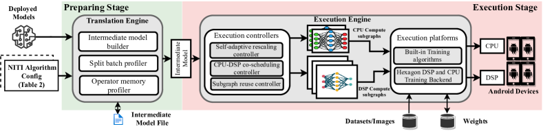
Figure 3. The overall workflow of Mandheling.

3. The Design

Mixed-precision algo.	W	A	G	WU	support
NITI (wang2020niti, )	INT8	INT8	INT8	INT8	$\checkmark$
Octo (zhou2021octo, )	INT8	INT8	INT8	INT8	$\checkmark$
Adaptive Fixed-Point (zhang2020fixed, )	INT8/INT16	INT8	INT8	FP32	$\checkmark$
WAGEUBN (yang2020training, )	INT8	INT8	INT8	FP24	$\checkmark$
MLS Format (zhong2020towards, )	INT8	INT8	INT8	FP32	$\checkmark$
Chunk-based (wang2018training, )	FP8	FP8	FP8	FP16	$\times$
Unified INT8 Training(zhu2020towards, )	INT8	INT8	INT8	FP32	$\times$
”W”, ”A”, ”G”, and ”WU” represent weight, activation, gradient and weight update.

Table 1. Data types of mixed-precision training algorithms.

Attribute	Contents
	key	value
Translation	FP32 Conv	INT8 Conv+ReduceMax+Shift
	FP32 MaxPool	INT8 MaxPool
Backprop.	FP32 Conv Error Grad.	INT8 Deconv
	FP32 Conv Weight Grad.	INT8 ConvBackpropFilter
Weight	Initializer	Xavier_normal
	Type	INT8
	Update	INT8
Optimizer	Loss	Cross Entropy
	Optimizer	SGD

Table 2. A typical NITI algorithm training config.

3.1. Overview

Design goal Mandheling aims to minimize the latency and energy consumption under a given training task through on-device DSP offloading. Mandheling is designed as a generic framework to support different kinds of mixed-precision algorithms and allows users to customize the algorithms through its exposed abstraction and configurations as will be discussed in $\S$3.2. The convergence accuracy is guaranteed by the used mixed-precision training algorithm.

Workflow. Figure 3 illustrates the workflow of Mandheling. The input of Mandheling includes the mixed-precision training algorithms and the model file that can be either pre-trained or randomly initialized. Once Mandheling is deployed on a device, it works in two following stages: (1) At the preparing stage, Mandheling translates models from different front-end frameworks (e.g., TensorFlow (tensorflow, ) and PyTorch (pytorch, )) to intermediate models in form of FlatBuffer-format model file. (2) At the execution stage, Mandheling generates CPU and DSP compute subgraphs and performs compute subgraphs execution on Android devices. Note that both stages run on devices, and the preparation stage is automatically triggered before the first-time execution of one shot. Hence, such a design does not introduce any additional programming efforts to the app developers.

• Preparing stage. When a to-be-trained model is downloaded to a device, Mandheling translates the model to an intermediate model via the Intermediate Model Builder according to mixed-precision training configuration. The intermediate model contains the operator’s type, hyperparameters, inputs and outputs as well as the memory regions of intermediate model inputs and outputs. Then, Mandheling runs a profiling iteration to obtain each layer’s optimal configuration via Split Batch Profiler to further optimize intermediate model to gain higher performance as to be shown in $\S$3.5. Lastly, a FlatBuffer format model file will be generated to be processed directly by the Mandheling runtime.

• Execution stage. Once a training task starts, Mandheling runtime first loads datasets and weights from disk to the required memory regions, and then generates CPU and DSP compute subgraphs via CPU-DSP co-scheduling controller ($\S$3.3). All subgraphs will execute on Android devices’ CPU or DSP via Mandheling’s Hexagon DSP and CPU Training backend, which includes operator implementation optimized for mixed-precision data types on CPU and DSP.

Key techniques. While DSP has been proven to be useful in DNN inference (lee2019mobisr, ), we observe a disparity between using DSP to serve training and inference tasks. Compared to the CPU, a vanilla DSP training engine can achieve very limited or even negative performance gain. To this end, Mandheling incorporates four key techniques to unleash the DSP computing capacity. The techniques can be divided into two major classes: intra-operator and inter-operator. At the intra-op level, since convolution and weight gradient layers will bring excessive memory access and exhaust the DSP cache, we use self-adaptive rescaling ($\S$3.4) and batch splitting ($\S$3.5) to reduce memory access and increase the cache hit ratio. At the inter-op level, Mandheling overlaps the CPU and DSP execution as much as possible to mitigate the overhead of DSP-unfriendly operators ($\S$3.3), and reuses DSP compute graph to eliminate the preparation overhead ($\S$3.6).

3.2. Mixed-Precision Training Abstraction

We thoroughly investigate the typical mixed-precision training algorithms (wang2020niti, ; zhou2021octo, ; wu2016binarized, ; lin2015neural, ; rastegari2016xnor, ; zhou2018adaptive, ; lin2017towards, ; courbariaux2015binaryconnect, ; jacob2018quantization, ; zhou2016dorefa, ) and summarize how they manipulate data in Table 2. We extract the basic concepts from those algorithms and identify 4 key elements that jointly define a mixed-precision training algorithm.

• Translation from FP32 operators to mixed-precision operators. To support an end-to-end training with mixed precision, a normal FP32 operator often needs to be translated into a combination of new operators that operate on data with different kinds of precision. Such translation is elaborately designed by algorithm developers to ensure good accuracy. Note that Mandheling has implemented lots of mixed-precision operators internally.

• Backpropagation rules are used to illustrate how to calculate operators’ weight and error gradients. For instance, the NITI algorithm uses INT8 deconvolution to calculate the FP32 convolution error gradients.

• Weight information includes weight type, weight initializing methods, and weight update algorithms.

• Optimizer information includes the loss function (e.g., cross entropy) and the optimizer, like SGD and ADAM.

Table 2 gives an example of how to use the above abstraction to specify the NITI algorithm. For example, an FP32 convolution needs to be translated into: (1) an INT8-based convolution; (2) a Max operation to obtain the scale factor; (3) a Shift operation to convert INT32 value to INT8 type. Such a configuration will be an input of Mandheling along with the model to be trained. Currently, Mandheling has already incorporated many built-in mixed-precision training algorithms, i.e., 5 out of 7 in Table 2. The other two are currently not supported yet due to the lack of support for the certain low-precision operator such as FP8-based convolution, and will be considered in future work.

Latency compare	Op	CPU	DSP
	Transpose	3 ms	25 ms
	WeightRotate	4 ms	20 ms
	Slice	4 ms	17 ms
DSP unsuppoted ops	Normalization, Quantization, Round, Sqrt, etc.

Table 3. Operators that do not fit to DSP.

3.3. CPU-DSP Co-Scheduling

DSP-unfriendly operators Though the DSP is adequate to INT8 vector arithmetic operations, there are still some irregular memory access operations or float operations that are unsuitable for DSP to run, referred to as “DSP-unfriendly operators” in this work. As shown in Table 3, some operators’ latency on DSP is more than 8$\times$ slower than that on CPU, and some FP32-only operators, such as Normalization and Quantization, are lack of architecture-level support on DSP (wang2020niti, ; yang2020training, ). Therefore, they need to be executed on the CPU.

To partition the model across DSP and CPU, an intuitive approach is to merge the adjacent DSP-unfriendly operators into subgraphs and place them on the CPU. However, since the CPU-DSP context switching incurs high overhead mainly due to the data copy between their own memory space (i.e., around 25ms on XiaoMI 10), this approach could lead to non-optimal performance. Conceptually, some DSP-friendly operators shall be placed on the CPU as well to reduce the CPU-DSP context switch frequency. Therefore, we need a context-switching-aware scheduling strategy that wisely maps the operators to CPU and DSP.

Operator-to-hardware scheduling To solve the scheduling problem, Mandheling first uses topological sort to get an execution order for all operators and profiles to obtain each operator’s latency on CPU and DSP. Then, it uses dynamic programming algorithm to find the approximately optimal scheduling solution while obeying the execution order.

(1) $$T[i+1,CPU]=min\left\{\begin{matrix}T[i,CPU]+L_{i+1}^{CPU}\\ T[i,DSP]+L_{i+1}^{CPU}+L_{switch}\end{matrix}\right.$$

(2) $$T[i+1,DSP] =min\left\{\begin{matrix}T[i,CPU]+L_{i+1}^{DSP}+L_{switch}\\ T[i,DSP]+L_{i+1}^{DSP}\end{matrix}\right.$$

$T[i+1,CPU]$ is the lowest latency of finishing $Op_{1}.....Op_{i+1}$ if $Op_{i+1}$ running on CPU. $L_{i+1}^{CPU}$ means the latency of $Op_{i+1}$ running on CPU and $L_{switch}$ represents the latency of context switching. The init state is set to $T[1,CPU]=L_{1}^{CPU}$ and $T[1,DSP]=L_{1}^{DSP}$. When both $Op_{i+1}$ and $Op_{i}$ running on CPU, there is no context switching. Otherwise, context switching overhead is added. $T[i+1,CPU]$ is the minimum value of the above two. Similarly, the latency of finishing $Op_{i+1}$ running on DSP also has two circumstances as shown in Eq 2. The objective $T_{model}$ can be formulated as

(3) $$T_{model}=min\{T[N,CPU],T[N,DSP]\}.$$

N is the number of operators. Based on the recursion formula and the objective, we can find the optimal scheduling plan. Note that the subgraphs can run on CPU and DSP in parallel, as long as their data dependency is satisfied.

3.4. Self-Adaptive Rescaling

⬇

1 int scale = 0;

2 /*Calculate INT32 temporal results*/

3 for(int i = 0; i < length; i++ ) {

4 Tensor x = input[i];

5 Tensor w = weight[i];

6 // CONV or matrix multiply

7 Tensor temp_result = x * w;

8 // count leading zero

9 Tensor clz = clz(temp_result);

10 int tscale = 32 - max(clz) - 7;

11 scale = scale > tscale? scale: tscale;

12 temp_output[i] = temp_result;

13 }

14 /* Cast the INT32 to INT8 values */

15 for(int i = 0; i < length; i++ ) {

16 Tensor temp = temp_output[i];

17 // Downscale

18 Tensor int8_result = temp / scale;

19 result[i] = int8_result;

20 }

Listing 1: Key C code snippet of dynamic rescaling

⬇

1 scale = 0

2

3loop0:

4 v0 = vmem ptr_i

5 v1 = vmem ptr_w

6

7 v2 = vrmpy v0, v1

8

9 v3 = vclz v2

10 tscale = vmax v3

11 scale = mux scale > tscale, scale,tscale

12 vmem ptr_t, v2

13end loop0

14loop1:

15 v0 = vmem ptr_t

16

17 v3 = vmpye v0, scale

18 vmem ptr_v, v3

19end loop1

Listing 2: Asm code version

Static scaling vs. dynamic rescaling Once a quantized model is deployed for inference, the scale factor (i.e., $S_{a}^{(l)}$ and $S_{w}^{(l)}$ in Figure 2) per layer is a static value. Therefore, the data flow is simple as it just needs to multiply the matrix after loading the input and weight, and store the scaled result. During training, however, the scale factor also needs to be dynamically adapted just like the trainable weights. An unreasonable scale factor can noticeably drop the model accuracy and the optimal scale factor cannot be known in prior to training completeness.

Mismatch of dynamic rescaling and DSP Such dynamic scaling runs slow on DSP for its excessive memory access. For each batch of training, we have to store the temporal outputs and reload them after obtaining the scale factor to downscale the temporal outputs to final INT8 results, as shown in Listing LABEL:code:dynamic-rescaling-c and LABEL:code:dynamic-rescaling. Note that each layer with trainable weights collocates with a scale factor. Therefore, there can be at most hundreds of dynamic scale factors in a typical DNN model. As we have measured, dynamic rescaling will at least add 2$\times$ latency compared with a static one.

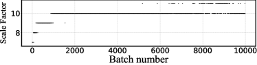
(a) Layer’s scale factor

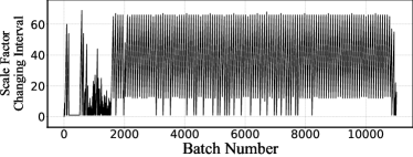
(b) Layer’s scale factor changing interval

Figure 4. The scale factor and its changing interval of the first CONV layer in training VGG11 model (batch size = 64) on CIFAR-10 dataset.

Insights & Opportunities Fortunately, we observed two useful patterns of how scale factors changes during training. Figure 4 illustrates (a) the concrete value of a scale factor of one layer and (b) its changing frequency in training the VGG11 model on CIFAR-10 dataset. We find that, after the initialization period: (1) The scale factor jumps between 2 alternative values, i.e., 10 and 11. Using either of them does not affect the model accuracy. (2) The actual changing frequency of the scale factor is low, e.g., per 10–60 batches. Those two phenomenons are common in training because when the model approaches to convergence, the gradients decrease and the scale factor is less likely to be changed.

Based on the above observations, we propose self-adaptive rescaling technique to mitigate the overhead of rescaling. Its key idea is to periodically enable the rescaling instead of per batch. The rescaling frequency is adaptively configured based on the observed history of how frequent the scale factors actually change after training, e.g., last $K$ batches with rescaling enabled. We heuristically set the policy in mapping the observed frequency of changed scale factor $f$ to the periodic frequency in calculating the new scale factor $f/2$. Luckily, we find such a policy works well for different kinds of models and datasets.

Input Size	latencies of different batch sizes (ms)
	2	4	8	16	32	64
8$\times$8	0.63	0.63	0.85	1.03	1.27	1.84
16$\times$16	0.84	0.89	4.23	3.98	4.64	12.24
32$\times$32	1.69	2.50	59.11	62.35	68.13	152.89

Table 4. The latency of a convolution layer on DSP with different batch/input sizes (input channel = 64, output channel = 64).

3.5. Batch Splitting

Exhausted data cache A well-known factor towards fast on-device inference is to fully utilize the processor cache (wang2021asymo, ). For inference tasks, using a large batch is very likely to improve the CPU utilization and, therefore, the processing throughput (smith2017don, ; goyal2017accurate, ). However, for DSP-based training tasks, we observe a huge performance decline on the large operator and batch sizes, especially for weight gradients calculation. Table 4 illustrates this phenomenon with a convolution operator on XiaoMI 10 (Snapdragon 865 SoC). When the input data size is 32$\times$32, the latency of batch size = 32 is 27.3$\times$ more than that of batch size = 4, which means 8$\times$ theoretical workload incurs 27.3$\times$ delay .

The performance drop comes from the exhausted DSP cache. There are two reasons for the disparate behavior on training and inference tasks. First, training tasks often require a large batch size, which leads to numerous amounts of memory access for intermediate data. Second, DSP cache is often smaller than CPU cache, e.g., only half for L2 cache on Snapdragon 865 (1 MB vs. 2 MB).

To reach a high cache hit ratio, we need to partition the intra-operator workloads. We choose to split the operation at the batch dimension, i.e., the first dimension of input data, as it is simpler to implement and causes no redundant computations. We refer an operator to behave “abnormal” if its latency-to-workload (in FLOPs) ratio is noticeably higher than the same configuration but with a smaller batch size. Through offline profiling, like we have done in Table 4, Mandheling can identify all abnormal operators in a model and split them into normal ones.

To ensure efficient locality, Mandheling splits an abnormal batch into multiple micro-batches and executes them individually. The final weight gradients are the accumulation of their output. The accumulation formula for FP32 operations is $W^{g}=\sum^{n}_{i=1}W^{g}_{batch_{i}}$. When comes to INT8, the formula will be changed into $W^{g}*S^{g}=\sum^{n}_{i=1}W^{g}_{batch_{i}}*S^{g}_{batch_{i}}$. This formula can be finally transformed to

(4) $$W^{g}=\sum^{n}_{i=1}W^{g}_{batch_{i}}*S^{g}_{batch_{i}}/S^{g}$$

According to Eq 4, if $S^{g}_{batch_{*}}/S^{g}=1$, we can avoid the FP32 add operation. Refer to non-split gradient algorithm, we can know that $S^{g}=max\{S^{g}_{batch_{i}},i\in split\_num\}$. Therefore, all the temporary micro-batch results should rescale from $S^{g}_{batch_{i}}$ to $S^{g}$. Our experiments show that when splitting the batch, in most cases $S^{g}_{batch_{i}}$ is the same as $S^{g}$, so rescaling will not compromise the benefits from batch splitting.

3.6. Compute Subgraph Reuse

Costly compute graph preparation Our experiments also show that preparing the compute graph takes a considerable amount of time, e.g., 304ms on TFLite and 212ms on MNN for the VGG16 (simonyan2014very, ) model, respectively. The preparation includes the following steps. First, the training engine needs to build the DSP compute subgraph, which consists of operators with inputs, outputs, and parameters. To ensure that the subgraph can execute correctly, the engine also maintains a reference relationship graph between operators. Before invoking the DSP training, the memory space needs to be allocated on DSP as well. The current on-device training engines always prepare a new compute subgraph for each batch of training. The dynamic graphs are rather easy for developers to debug and develop, however, unfortunately they incur high overhead on resource-constrained devices, which are not suitable for on-device training.

Since the models are rarely modified during on-device training, we propose to reuse the DSP compute subgraph to eliminate its preparation overhead. However, directly reusing the subgraph can easily exceed the DSP memory budget since substantial memory regions cannot be released. To this end, Mandheling seeks to minimize the memory allocation/deallocation operations under the memory constraint – a common memory management problem in the operating system (zhao2005dynamic, ; pyka2007operating, ; tiwari2010mmt, ; beyler2007performance, ). An opportunity is that, unlike OS, Mandheling’s memory allocation/deallocation for subgraph reuse always follows DNN’s execution order, so that the memory region most recently used (MRU) has the longest reuse distance. Therefore, the key idea is to release the MRU memory regions which best fit memory needs.

• At the preparing stage, Mandheling profiles all memory regions that compute subgraphs use as shown in Figure 3. Since the number of compute subgraphs is rather small ($<$100), we can exhaustively explore all circumstances to find all possible solutions satisfying different requiring memory sizes.

• When the system is about to exceed the memory budget, Mandheling releases the MRU memory regions identified and marked at the preparing stage, and allocates space for newly coming subgraphs.

4. Implementation and Evaluation

We have fully implemented Mandheling with 15k LoC in C/C++ and 800 LoC of assembly language in total. The prototype is a standalone framework supporting models exported from MNN (mnn, ), TFLite (tflite, ), and Pytorch Mobile (pytorch, ). Mandheling leverages Hexagon NN (hexagon-nn, ) as the DSP backend, which is the only open-source library supporting inference on DSP developed by Qualcomm. While Mandheling has supported many different mixed-precision training algorithms as shown in Table 2, in our experiments, we use NITI (wang2020niti, ) as the default one, because it extensively uses INT8 operations that are quite suitable for DSP. Since Hexagon DSP architecture is constantly changing, we mainly optimize our implementation for V66 architecture through assembly code. The prototype reuses the FP32-based operators running on the CPU from MNN.

4.1. Experimental Methodology

Devices	CPU	GPU	DSP
XiaoMI 11 Pro Snapdragon 888	2.84GHz Cortex-X1	Adreno 660 GPU 700MHz	Hexagon 780 DSP 500MHz
	3$\times$ 2.4GHz Cortex A78
	4$\times$ 1.8GHz Cortex A55
XiaoMI 10 Snapdragon 865	2.84GHz A77	Adreno 650 GPU 587MHz	Hexagon 698 DSP 500MHz
	3$\times$ 2.4GHz Cortex A77
	4$\times$ 1.8GHz Cortex A55
Redmi Note9 Pro Snapdragon 750G	2$\times$ 2.2GHz Cortex A77 6$\times$ 1.8GHz Cortex A55	Adreno 619 GPU 950MHz	Hexagon 694 DSP 500MHz

Table 5. Devices used in the experiments.

Model	Input Data	FLOPs	# of CONVs
VGG-11 (simonyan2014very, )	CIFAR-10	914 M	8
VGG-16 (simonyan2014very, )	CIFAR-10	1.35 G	13
VGG-19 (simonyan2014very, )	ImageNet	26.92 G	16
ResNet-34 (he2016deep, )	CIFAR-10	7.26 G	36
ResNet-18 (he2016deep, )	ImageNet	11.66 G	20
InceptionV3 (szegedy2016rethinking, )	CIFAR-10	2.43 G	16

Table 6. DNN models used in the experiments.

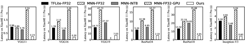
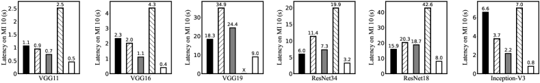
Figure 5. Per-batch training time on different models (batch size = 64) on different devices.

Hardware setup. We test the performance of Mandheling on three smartphones with different Qualcomm SoCs: XiaoMI 11 Pro (Snapdragon 888), XiaoMI 10 (Snapdragon 865), and Redmi Note9 Pro (Snapdragon 750G). The XiaoMI 11 Pro device is equipped with the latest Hexagon 780 DSP, which is claimed to have huge performance promotions over the old ones. The hardware details are shown in Table 5. All devices run Android OS 10. By default, we always run the baselines on 4 BIG CPU cores and Mandheling’s CPU workloads on 2 BIG cores. The CPU frequency is controlled by OS’s dynamic voltage and frequency scaling (DVFS) controller.

Models. We test with a range of typical CNN models with various input sizes: VGG11/16/19 (simonyan2014very, ), ResNet18/34 (he2016deep, ), and InceptionV3 (szegedy2016rethinking, ), as listed in Table 6. The input data to those models are either CIFAR-10 (krizhevsky2009learning, ) (input size 32x32) or ImageNet (krizhevsky2012imagenet, ) (input size 224x224).

Baselines. We mainly compare Mandheling with two frameworks. One is MNN (mnn, ) that is one of the earliest frameworks that has supported on-device training since late 2019. Note that Mandheling also reuses some operator implementation from MNN. The other one is TFLite (tflite, ), which is the most popular DL framework on smartphones and lately added training support in November, 2021. Both MNN and TFLite only support training with FP32 format. To make a more fair comparison, we also extend MNN to train with INT8 format using the same training algorithm as Mandheling on CPU. More specifically, we compare Mandheling with four baselines: (1) TFLite-FP32: the traditional FP32-based training method provided by TFLite. (2) MNN-FP32: the traditional FP32-based training method provided by MNN. (3) MNN-INT8: the INT8-based training method implemented by us based on MNN. NEON (reddy2008neon, ) is extensively used to optimize the performance of this baseline. (4) MNN-FP32-GPU: FP32-based training on mobile GPU through OpenCL backend.

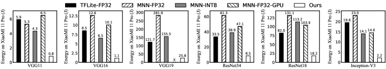
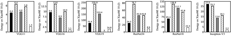
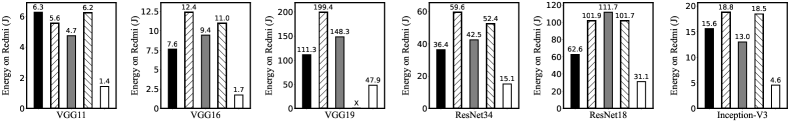
Figure 6. Per-batch energy consumption on different models (batch size = 64) on different devices.

Metrics and configurations. We mainly measure the training time and energy consumption during training. The energy consumption is calculated through Android’s vFS (/sys /class/power_supply) by profiling every 100ms. Besides, we also evaluate thermal and CPU frequency through /sys/ class/thermal/thermal_zone and /sys/devices/system/ cpu/cpufreq to show our power efficiency from long duration of intensive computation. All experiments are repeated by 3 times and the average numbers are reported.

4.2. Per-Batch Performance

Overall performance We first comprehensively investigate the per-batch training performance of Mandheling with batch size 64. The latency and energy consumption results are illustrated in Figure 5 and Figure 6, respectively. Our key observation is that Mandheling consistently and remarkably outperforms other baselines on both metrics.

• Training latency of Mandheling vs. FP32 baselines Compared with MNN-FP32 and TFLite-FP32, Mandheling achieves 2.08-7.1$\times$ and 1.44-8.25$\times$ speedup of per-batch training time, respectively. Comparing different devices, we observe that Mandheling’s improvements are relatively less profound on Redmi Note9 Pro than the other two devices. This is because Redmi Note9 Pro is equipped with an outdated SoC where the performance gap between CPU and DSP is much smaller than the other two high-end SoCs.

• Energy consumption of Mandheling vs. FP32 baselines As Figure 6 shows, Mandheling’s improvements on energy consumption are even more profound than training speed. Specifically, Mandheling reduces the energy consumption by 3.21-11.2$\times$ and 2.01-12.5$\times$ compared with MNN-FP32 and TFLite-FP32, respectively. Such a huge benefit comes from both the training speedup and the higher power efficiency of DSP.

• Mandheling vs. MNN-FP32-GPU Mandheling can reduce 3.98-11.63$\times$ latency and 3.46-10.95$\times$ energy consumption compared with MNN-FP32-GPU. The reason for such huge improvement is that (1) As far as we know, MNN is the only framework supporting on-device GPU training and is not fully optimized yet. The GPU utilization during training is only around 30-50%. (2) DSP is more power-efficient than GPU. Besides, training the VGG19 model on ImageNet with MNN-FP32-GPU encounters out-of-memory failure.

• Mandheling vs. MNN-INT8 According to Figure 5 and Figure 6, Mandheling can reduce up to 4.13$\times$ latency and 6.5$\times$ energy consumption compared to MNN-INT8, respectively. Since both of them use the same mixed-precision training algorithm, the improvements come from Mandheling’s ability to fully utilize the DSP hardware. Note that DSP HVX vector instruction can at most calculate 128 INT8 arithmetic operations; while CPU NEON can only perform 4 operations.

Impacts of batch size

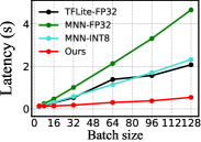
(a) VGG16 Latency

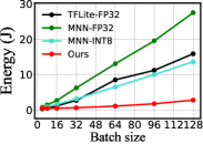
(b) VGG16 Energy

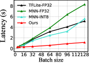
(c) InceptionV3 Latency

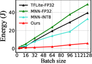
(d) InceptionV3 Energy

Figure 7. Per-batch training time and energy consumption under various batch sizes.

We then evaluate the performance of Mandheling with various batch sizes from 4 to 128 with VGG16 and InceptionV3 models on XiaoMI 11 Pro. As shown in Figure 7, Mandheling consistently outperforms other baselines on each batch size, e.g., 4.81$\times$ lower latency and 6.90$\times$ lower energy consumption on average. Besides, the performance gap between Mandheling and baselines is bigger with batch size increasing. For instance, Mandheling reduces up to 8.56$\times$ latency and 12.67$\times$ energy consumption for batch size 128 thanks to the batch splitting technique ($\S$3.5).

Impacts of CPU cores

Method	CPU Conf.	Time (s)		Energy (J)
		H	L	H	L
MNN-FP32	BIG 1$\times$	4.88	10.81	11.05	6.90
	BIG 2$\times$	2.87	5.89	12.85	7.50
	BIG 4$\times$ (default)	2.14	3.86	11.90	7.10
	LITTLE 1$\times$	25.20	42.57	13.35	21.95
	LITTLE 4$\times$	10.75	17.06	14.85	9.55
	Hybrid 8$\times$	4.50	7.58	25.40	12.45
MNN-INT8	BIG 1$\times$	5.59	14.75	9.85	4.35
	BIG 2$\times$	3.07	7.37	10.60	5.25
	BIG 4$\times$ (default)	1.79	3.8	7.90	4.55
	LITTLE 1$\times$	40.13	81.20	12.65	25.85
	LITTLE 4$\times$	10.36	20.64	10.35	5.95
	Hybrid 8$\times$	2.71	4.96	12.10	6.20
Ours	BIG 1$\times$	0.29	0.41	0.70	0.65
	BIG 2$\times$ (default)	0.25	0.32	0.90	0.70
	BIG 4$\times$	0.24	0.31	1.20	0.90
	LITTLE 1$\times$	0.79	1.61	0.80	1.15
	LITTLE 4$\times$	0.49	0.68	0.90	0.75
	Hybrid 8$\times$	0.34	0.39	1.60	0.90

Table 7. The performance impacts from the selection of CPU cores and their frequency (H/L: highest/lowest frequency available). Numbers in highlight indicate the best performance or least energy consumption.

Since most baselines and part of Mandheling runs on CPUs, it’s intuitive to test how the choice of CPU cores affect their performance. In this experiment we use the VGG16 model with batch size 64. We vary the CPU core numbers and the frequency for each core on XiaoMI 11 Pro. The results are summarized in Table 7.

As observed, the choice of CPU cores opens rich tradeoffs for Mandheling and baselines between the training speed and energy consumption. Running on 4 BIG CPU cores with the highest frequency enables Mandheling to train with the fastest speed (0.24s per batch), yet its energy consumption is 1.9$\times$ higher than 1 BIG CPU core with the lowest frequency. The default configuration for Mandheling is to use 2 BIG CPU cores with DVFS to make a balance between the two key metrics. In reality, a developer or the OS might control the CPU cores to harness such a tradeoff. For instance, on a low-power device, the OS might signal Mandheling to use only one BIG CPU core for training. To be noted, Mandheling still significantly outperforms other baselines with any settings.

4.3. End-to-End Convergence

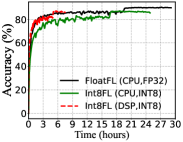
(a) VGG11-CIFAR10-Local

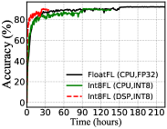
(b) ResNet18-CIFAR10-Local

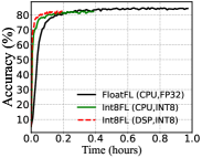
(c) LENET-FEMNIST-Federated

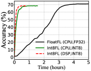
(d) VGG16-CIFAR100-Federated

Figure 8. The convergence accuracy across clock time under single device and federated scenarios.

Dataset	Model	Methods	Acc.	Training Cost to Convergence
				Round number	Clock Hours	Energy (WH)
Centralized CIFAR-10	VGG11	MNN-FP32	89.87%	150	29.13	187.01
		MNN-INT8	87.17%	150	24.77	153.33
		Ours	87.17%	150	7.50	31.39
Centralized CIFAR-10	ResNet18	MNN-FP32	92.49%	150	223.55	1,435.19
		MNN-INT8	90.62%	150	135.71	840.04
		Ours	90.62%	150	35.68	149.32
Federated FEMNIST	LeNet	MNN-FP32	84.18%	990	0.97	0.00057
		MNN-INT8	82.04%	4,960	0.39	0.00029
		Ours	82.04%	4,960	0.19	0.00007
Federated CIFAR-100	VGG16	MNN-FP32	71.15%	1,960	8.35	2.74
		MNN-INT8	68.42%	2,200	1.56	1.26
		Ours	68.42%	2,200	0.78	0.21

Table 8. A summary of end-to-end training cost till convergence under different training scenarios.

We now demonstrate that Mandheling is able to significantly accelerate the model convergence while guaranteeing the model accuracy in end-to-end training experiments. We focus on the time-to-accuracy metric (wang2020niti, ; yang2020training, ; zhong2020towards, ; zhang2020fixed, ; zhu2020towards, ).

Learning on a single device is the case when all training data resides in a single device. We train VGG16 and ResNet18 with training set CIFAR-10 on XiaoMI 11 Pro and verify the accuracy after each epoch. We fix the CPU frequency to the max value and 10 minutes sleep after training 10 epochs to avoid shutting down due to overheating. Note that sleep time does not count in the time-to-accuracy.

As illustrated in Figure 8(a) and (b) and summarized in the first two rows of Table 8, the convergence accuracy of Mandheling is only 1.9-2.7% lower than training with FP32. This accuracy drop is consistent with the numbers reported by the original algorithm paper (wang2020niti, ), and are generally acceptable by the relevant ML community (wang2020niti, ; zhou2021octo, ; wu2016binarized, ; lin2015neural, ; rastegari2016xnor, ; zhou2018adaptive, ; lin2017towards, ; courbariaux2015binaryconnect, ; jacob2018quantization, ; zhou2016dorefa, ; banner2018scalable, ; chen2017fxpnet, ; wu2018training, ; zhu2016trained, ; wang2018training, ; zhu2020towards, ; zhang2020fixed, ; yang2020training, ; zhong2020towards, ). However, it only takes 5.06-6.27$\times$ less time and 5.96-9.62$\times$ less energy consumption for Mandheling to the convergence accuracy (87.17% and 90.40%) compared with MNN-FP32. Compared to MNN-INT8, Mandheling converges to the same accuracy as they both use NITI training algorithm, but takes 3.55$\times$ less time and 5.46$\times$ less energy consumption on average.

Cross-device federated learning is another killer use case that allows many devices to collaboratively train a model without giving away their training data. In our experiments, we use a popular FL simulation platform (yang2021characterizing, ) and plug in the tested on-device training performance of Mandheling and baselines into the platform. Both FloatFL and Int8FL use the traditional FL protocol FedAvg. For a fair comparison, we set the number of the local epoch as 1 for all experiments. We use FEMNIST (reddi2020adaptive, ) and CIFAR-100 (krizhevsky2009learning, ) as the testing datasets, and follow prior work (he2020fedml, ) to partition them into non-IID distribution.

As demonstrated in Figure 8(c) and (d) and the last three rows of Table 8, the accuracy of Mandheling is 2.14% and 2.73% lower than FLoatFL on FEMNIST and CIFAR-100, respectively. However, it only takes 19.58% and 9.3% of clock time to converge (i.e., 5.26$\times$ and 10.75$\times$ speedup) with Mandheling, respectively. Such tremendous improvement over FloatFL protocol comes from both reduced on-device training time and communication time of applying INT8-based training. As Table 8 also shows that Mandheling reduces 8.14$\times$, and 13.1$\times$ energy consumption of single client, respectively.

Thermal impacts

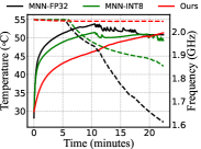
(a) XiaoMI 11 Pro

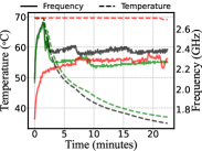
(b) XiaoMI 10

Figure 9. The temperature and CPU frequency dynamics during on-device training on different devices.

To reach a usable accuracy, the on-device training often takes a substantial amount of time (bonawitz2019towards, ), e.g., minutes for each round of federated learning or even hours for continuous local transfer learning (deeptype, ). Such a long duration of intensive computation may lead to thermal issues and, therefore, the CPU frequency change due to DVFS. Thus we investigate the thermal dynamics of on-device training on two devices and illustrate the results in Figure 9. On both tested devices, we observe the temperature rising and the CPU underclocking, but the trend for Mandheling is much milder than the other two baselines. Using MMN-FP32 and XiaoMI 10 as an example, the device temperature rises sharply from 29°C to 68°C in 2 minutes, and the CPU frequency drops from 2.8GHz to 1.3GHz. On the other hand, it takes about 18 minutes for Mandheling to raise the temperature from 29°C to 58°C which leads to almost no CPU underclocking. This is because DSP frequency is 4$\times$ lower than CPU and is designed for low-power scenarios.

4.4. Ablation Study

Figure 10. Ablation study of Mandheling.

We further conduct a breakdown analysis of the benefit brought by Mandheling’s each technique. The experiments are performed with VGG11, VGG16 and ResNet34 models on XiaoMI 10. The results are illustrated in Figure 10.

We observe that all techniques have non-trivial contribution to the improvement. For instance, the per-bach training time for ResNet34 model is 27.68s without any optimizations. When the self-adaptive rescaling is applied, the latency reduces to 13.02s. Adding the compute subgraph reusing technique further decreases the latency to 4.54s. The other two techniques, i.e., batch splitting and CPU-DSP parallel execution, also add to 22.9% and 19.5% lower latency, respectively. Since the 4 key techniques optimize the training cost from different aspects, they can well orchestrate to provide accumulative optimization. Besides, the profits of batch splitting for VGG11 is rather small compared with other two models. That is because the workload of VGG11 model is smaller so we do not observe high cache pressure that motivates the batch splitting technique.

4.5. Fitting to Various Training Algorithms

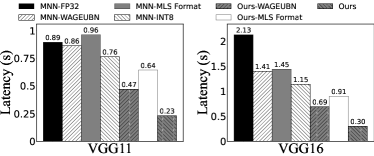
(a) Latency

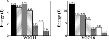
(b) Energy consumption

Figure 11. Mandheling’s performane using different mixed-precision training algorithm. ”MNN-*” are baselines runing on CPU; while ”Ours-*” are runing on DSP using Mandheling.

Recall that Mandheling is an underlying independent framework that supports different kinds of mixed-precision training algorithms. Therefore we also test Mandheling with different training algorithms: NITI (wang2020niti, ) (default), MLS Format (zhong2020towards, ), and WAGEUBN (yang2020training, ). The experiments are performed with VGG11 and VGG16 on XiaoMI 11 Pro.

As shown in Figure 11, the training speed of three mixed-precision algorithms are all faster than that of MNN-FP32 (3.08$\times$, 2.34$\times$, and 7.1$\times$ speedup). The energy consumption improvement of Mandheling is more significant, i.e., 3.64$\times$ and 6.85$\times$ average reduction for VGG11 and VGG16, respectively. That is because Mandheling’s key techniques are aimed at solving the generic challenges to support different kinds of mixed-precision training algorithms. When comparing the same mixed-precision training algorithms running on CPU and DSP, Mandheling is still 2.04$\times$, 1.59$\times$, and 3.83$\times$ faster, respectively. Such benefit comes from Mandheling’s effective DSP offloading. Besides, among different training algorithms, NITI has the lowest training latency because it maximizes the usage of INT8 in its data flow.

5. Related Work

Mixed-precision DNN training Recently, many mixed-precision DNN training algorithms have been proposed to reduce the training cost (wang2020niti, ; zhou2021octo, ; wu2016binarized, ; lin2015neural, ; rastegari2016xnor, ; zhou2018adaptive, ; lin2017towards, ; courbariaux2015binaryconnect, ; jacob2018quantization, ; zhou2016dorefa, ; banner2018scalable, ; chen2017fxpnet, ; wu2018training, ; zhu2016trained, ). The key idea is to replace the default numerical format of FP32 with lower precision for activations and/or weights, e.g., FP16, INT8, or even BOOL type. Octo (zhou2021octo, ) further proposes an INT8-based training algorithm and also builts a system for edge GPUs. Instead of contributing new mixed-precision training algorithms, Mandheling is designed as an generic, underlying system to efficiently support those algorithms.

On-chip DNN offloading has been studied to enable faster DNN inference on heterogeneous mobile processors like GPU and DSP. Most of them focus on how to partition and schedule the workloads on different processors, such as intra-layer (kim2019mulayer, ; zeng2021energy, ), inter-layer (ha2021accelerating, ), block-layer level (lane2016deepx, ; han2019mosaic, ), and model level (zhang2020mobipose, ; lee2019mobisr, ; georgiev2014dsp, ). However, they only focus on DNN inference. Besides ML tasks, GPU/DSP are also leveraged for signal, sound and image processing (lane2015deepear, ; georgiev2017accelerating, ; rana2016opportunistic, ; liu2014imashup, ). Mandheling is motivated by those efforts, and is the first framework to support the offloading of training workloads to mobile DSP.

DNN inference optimizations Besides on-chip DNN offloading, there have many other research efforts in improving the DNN inference performance on devices. For instance, some apply structured pruning techniques to trade off latency and model accuracy (han2021legodnn, ; fang2018nestdnn, ; han2016mcdnn, ). Some improve the low-level kernel implementation through a compiler, core scheduling, etc (wang2021asymo, ; chen2018tvm, ; liu2019optimizing, ). Some of them optimize the DNN inference in specific scenarios (huynh2017deepmon, ; xu2018deepcache, ; yeo2020nemo, ; zhang2020mobipose, ). Mandheling is inspired by those work, yet focuses on training instead of inference. As previously discussed, DNN training faces many unique challenges as compared to inference, so Mandheling contributes novel techniques in addressing those challenges.

Federated learning is an emerging machine learning paradigm (konevcny2016federatedlearning, ; mcmahan2017communication, ; niu2020billion, ; mo2021ppfl, ) that is built atop on-device training and requires many clients to collaboratively train a DNN model. The communication bottleneck seriously affects the system efficiency and model accuracy (kairouz2021advances, ). Therefore, prior work mostly focus on model compression technique (jhunjhunwala2021adaptive, ; reisizadeh2020fedpaq, ; shlezinger2020federated, ; tang2018communication, ; li2021hermes, ) to reduce communication traffic. Others As an underlying framework, Mandheling is orthogonal and compatible with those algorithm-level optimizations.

6. Conclusions

In this paper, we have proposed Mandheling, the first system that enables highly resource-efficient on-device training by orchestrating the mixed-precision training with on-chip DSP offloading. Mandheling incorporated novel techniques such as self-adaptive rescaling and CPU-DSP co-scheduling to fully unleash the power of DSP. We conducted extensive experiments to evaluate Mandheling.

References

- [1] Federated learning: Collaborative machine learning without centralized training data. https://ai.googleblog.com/2017/04/federated-learning-collaborative.html, 2017.
- [2] How apple personalizes siri without hoovering up your data. https://www.technologyreview.com/2019/12/11/131629/apple-ai-personalizes-siri-federated-learning/, 2019.
- [3] Qualcomm hexagon nn offload framework. https://source.codeaurora.org/quic/hexagon_nn/, 2020.
- [4] dsp-processor. https://developer.qualcomm.com/software/hexagon-dsp-sdk/dsp-processor, 2021.
- [5] General data protection regulation. https://gdpr-info.eu/, 2021.
- [6] Genshin. https://genshin.mihoyo.com/, 2021.
- [7] /hexagon-dsp-sdk. https://developer.qualcomm.com/software/hexagon-dsp-sdk, 2021.
- [8] Qualcomm hexagon. https://en.wikipedia.org/wiki/Qualcomm_Hexagon, 2021.
- [9] Tiktok. https://www.tiktok.com, 2021.
- [10] Youtube. https://www.youtube.com, 2021.
- [11] Martín Abadi, Paul Barham, Jianmin Chen, Zhifeng Chen, Andy Davis, Jeffrey Dean, Matthieu Devin, Sanjay Ghemawat, Geoffrey Irving, Michael Isard, et al. Tensorflow: A system for large-scale machine learning. In 12th USENIX Symposium on Operating Systems Design and Implementation), pages 265–283, 2016.
- [12] Ron Banner, Itay Hubara, Elad Hoffer, and Daniel Soudry. Scalable methods for 8-bit training of neural networks. Advances in neural information processing systems, 31, 2018.
- [13] Jean Christophe Beyler and Philippe Clauss. Performance driven data cache prefetching in a dynamic software optimization system. In Proceedings of the 21st annual international conference on Supercomputing, pages 202–209, 2007.
- [14] Keith Bonawitz, Hubert Eichner, Wolfgang Grieskamp, Dzmitry Huba, Alex Ingerman, Vladimir Ivanov, Chloe Kiddon, Jakub Konečnỳ, Stefano Mazzocchi, H Brendan McMahan, et al. Towards federated learning at scale: System design. arXiv preprint arXiv:1902.01046, 2019.
- [15] Léon Bottou. Large-scale machine learning with stochastic gradient descent. In Proceedings of 19th International Conference on Computational Statistics, pages 177–186. Springer, 2010.
- [16] Tianqi Chen, Thierry Moreau, Ziheng Jiang, Lianmin Zheng, Eddie Yan, Haichen Shen, Meghan Cowan, Leyuan Wang, Yuwei Hu, Luis Ceze, et al. : An automated end-to-end optimizing compiler for deep learning. In 13th USENIX Symposium on Operating Systems Design and Implementation, pages 578–594, 2018.
- [17] Xi Chen, Xiaolin Hu, Hucheng Zhou, and Ningyi Xu. Fxpnet: Training a deep convolutional neural network in fixed-point representation. In 2017 International Joint Conference on Neural Networks, pages 2494–2501. IEEE, 2017.
- [18] Matthieu Courbariaux, Yoshua Bengio, and Jean-Pierre David. Binaryconnect: Training deep neural networks with binary weights during propagations. Advances in neural information processing systems, 28, 2015.
- [19] Biyi Fang, Xiao Zeng, and Mi Zhang. Nestdnn: Resource-aware multi-tenant on-device deep learning for continuous mobile vision. In Proceedings of the 24th Annual International Conference on Mobile Computing and Networking, pages 115–127, 2018.
- [20] Petko Georgiev, Nicholas D Lane, Cecilia Mascolo, and David Chu. Accelerating mobile audio sensing algorithms through on-chip gpu offloading. In Proceedings of the 15th Annual International Conference on Mobile Systems, Applications, and Services, pages 306–318, 2017.
- [21] Petko Georgiev, Nicholas D Lane, Kiran K Rachuri, and Cecilia Mascolo. Dsp. ear: Leveraging co-processor support for continuous audio sensing on smartphones. In Proceedings of the 12th ACM Conference on Embedded Network Sensor Systems, pages 295–309, 2014.
- [22] Priya Goyal, Piotr Dollár, Ross Girshick, Pieter Noordhuis, Lukasz Wesolowski, Aapo Kyrola, Andrew Tulloch, Yangqing Jia, and Kaiming He. Accurate, large minibatch sgd: Training imagenet in 1 hour. arXiv preprint arXiv:1706.02677, 2017.
- [23] Donghee Ha, Mooseop Kim, KyeongDeok Moon, and Chi Yoon Jeong. Accelerating on-device learning with layer-wise processor selection method on unified memory. IEEE Sensors, 21(7):2364, 2021.
- [24] Myeonggyun Han, Jihoon Hyun, Seongbeom Park, Jinsu Park, and Woongki Baek. Mosaic: Heterogeneity-, communication-, and constraint-aware model slicing and execution for accurate and efficient inference. In 2019 28th International Conference on Parallel Architectures and Compilation Techniques, pages 165–177. IEEE, 2019.
- [25] Rui Han, Qinglong Zhang, Chi Harold Liu, Guoren Wang, Jian Tang, and Lydia Y Chen. Legodnn: block-grained scaling of deep neural networks for mobile vision. In Proceedings of the 27th Annual International Conference on Mobile Computing and Networking, pages 406–419, 2021.
- [26] Seungyeop Han, Haichen Shen, Matthai Philipose, Sharad Agarwal, Alec Wolman, and Arvind Krishnamurthy. Mcdnn: An approximation-based execution framework for deep stream processing under resource constraints. In Proceedings of the 14th Annual International Conference on Mobile Systems, Applications, and Services, pages 123–136, 2016.
- [27] Andrew Hard, Kanishka Rao, Rajiv Mathews, Swaroop Ramaswamy, Françoise Beaufays, Sean Augenstein, Hubert Eichner, Chloé Kiddon, and Daniel Ramage. Federated learning for mobile keyboard prediction. arXiv preprint arXiv:1811.03604, 2018.
- [28] Chaoyang He, Songze Li, Jinhyun So, Xiao Zeng, Mi Zhang, Hongyi Wang, Xiaoyang Wang, Praneeth Vepakomma, Abhishek Singh, Hang Qiu, et al. Fedml: A research library and benchmark for federated machine learning. arXiv preprint arXiv:2007.13518, 2020.
- [29] Kaiming He, Xiangyu Zhang, Shaoqing Ren, and Jian Sun. Deep residual learning for image recognition. In Proceedings of the IEEE conference on computer vision and pattern recognition, pages 770–778, 2016.
- [30] Loc N Huynh, Youngki Lee, and Rajesh Krishna Balan. Deepmon: Mobile gpu-based deep learning framework for continuous vision applications. In Proceedings of the 15th Annual International Conference on Mobile Systems, Applications, and Services, pages 82–95, 2017.
- [31] Benoit Jacob, Skirmantas Kligys, Bo Chen, Menglong Zhu, Matthew Tang, Andrew Howard, Hartwig Adam, and Dmitry Kalenichenko. Quantization and training of neural networks for efficient integer-arithmetic-only inference. In Proceedings of the IEEE conference on computer vision and pattern recognition, pages 2704–2713, 2018.
- [32] Divyansh Jhunjhunwala, Advait Gadhikar, Gauri Joshi, and Yonina C Eldar. Adaptive quantization of model updates for communication-efficient federated learning. In 2021 IEEE International Conference on Acoustics, Speech and Signal Processing, pages 3110–3114. IEEE, 2021.
- [33] Xiaotang Jiang, Huan Wang, Yiliu Chen, Ziqi Wu, Lichuan Wang, Bin Zou, Yafeng Yang, Zongyang Cui, Yu Cai, Tianhang Yu, et al. Mnn: A universal and efficient inference engine. arXiv preprint arXiv:2002.12418, 2020.
- [34] Peter Kairouz, H Brendan McMahan, Brendan Avent, Aurélien Bellet, Mehdi Bennis, Arjun Nitin Bhagoji, Kallista Bonawitz, Zachary Charles, Graham Cormode, Rachel Cummings, et al. Advances and open problems in federated learning. Foundations and Trends® in Machine Learning, 14(1–2):1–210, 2021.
- [35] Youngsok Kim, Joonsung Kim, Dongju Chae, Daehyun Kim, and Jangwoo Kim. layer: Low latency on-device inference using cooperative single-layer acceleration and processor-friendly quantization. In Proceedings of the Fourteenth EuroSys Conference 2019, pages 1–15, 2019.
- [36] Jakub Konečnỳ, H Brendan McMahan, Felix X Yu, Peter Richtárik, Ananda Theertha Suresh, and Dave Bacon. Federated learning: Strategies for improving communication efficiency. arXiv preprint arXiv:1610.05492, 2016.
- [37] Alex Krizhevsky, Geoffrey Hinton, et al. Learning multiple layers of features from tiny images. 2009.
- [38] Alex Krizhevsky, Ilya Sutskever, and Geoffrey E Hinton. Imagenet classification with deep convolutional neural networks. Advances in neural information processing systems, 25, 2012.
- [39] Nicholas D Lane, Sourav Bhattacharya, Petko Georgiev, Claudio Forlivesi, Lei Jiao, Lorena Qendro, and Fahim Kawsar. Deepx: A software accelerator for low-power deep learning inference on mobile devices. In 2016 15th ACM/IEEE International Conference on Information Processing in Sensor Networks, pages 1–12. IEEE, 2016.
- [40] Nicholas D Lane, Petko Georgiev, and Lorena Qendro. Deepear: robust smartphone audio sensing in unconstrained acoustic environments using deep learning. In Proceedings of the 2015 ACM international joint conference on pervasive and ubiquitous computing, pages 283–294, 2015.
- [41] Royson Lee, Stylianos I Venieris, Lukasz Dudziak, Sourav Bhattacharya, and Nicholas D Lane. Mobisr: Efficient on-device super-resolution through heterogeneous mobile processors. In The 25th Annual International Conference on Mobile Computing and Networking, pages 1–16, 2019.
- [42] Ang Li, Jingwei Sun, Pengcheng Li, Yu Pu, Hai Li, and Yiran Chen. Hermes: an efficient federated learning framework for heterogeneous mobile clients. In Proceedings of the 27th Annual International Conference on Mobile Computing and Networking, pages 420–437, 2021.
- [43] Xiaofan Lin, Cong Zhao, and Wei Pan. Towards accurate binary convolutional neural network. Advances in neural information processing systems, 30, 2017.
- [44] Zhouhan Lin, Matthieu Courbariaux, Roland Memisevic, and Yoshua Bengio. Neural networks with few multiplications. arXiv preprint arXiv:1510.03009, 2015.
- [45] TensorFlow Lite. Deploy machine learning models on mobile and iot devices, 2019.
- [46] Xuanzhe Liu, Gang Huang, Qi Zhao, Hong Mei, and M Brian Blake. imashup: a mashup-based framework for service composition. Science China Information Sciences, 57(1):1–20, 2014.
- [47] Yizhi Liu, Yao Wang, Ruofei Yu, Mu Li, Vin Sharma, and Yida Wang. Optimizing cnn model inference on cpus. In 2019 USENIX Annual Technical Conference, pages 1025–1040, 2019.
- [48] Christos Louizos, Matthias Reisser, Tijmen Blankevoort, Efstratios Gavves, and Max Welling. Relaxed quantization for discretized neural networks. arXiv preprint arXiv:1810.01875, 2018.
- [49] Brendan McMahan, Eider Moore, Daniel Ramage, Seth Hampson, and Blaise Aguera y Arcas. Communication-efficient learning of deep networks from decentralized data. In Artificial intelligence and statistics, pages 1273–1282. PMLR, 2017.
- [50] Sparsh Mittal. A survey of recent prefetching techniques for processor caches. ACM Computing Surveys, 49(2):1–35, 2016.
- [51] Fan Mo, Hamed Haddadi, Kleomenis Katevas, Eduard Marin, Diego Perino, and Nicolas Kourtellis. Ppfl: privacy-preserving federated learning with trusted execution environments. In Proceedings of the 19th Annual International Conference on Mobile Systems, Applications, and Services, pages 94–108, 2021.
- [52] Chaoyue Niu, Fan Wu, Shaojie Tang, Lifeng Hua, Rongfei Jia, Chengfei Lv, Zhihua Wu, and Guihai Chen. Billion-scale federated learning on mobile clients: A submodel design with tunable privacy. In Proceedings of the 26th Annual International Conference on Mobile Computing and Networking, pages 1–14, 2020.
- [53] Adam Paszke, Sam Gross, Francisco Massa, Adam Lerer, James Bradbury, Gregory Chanan, Trevor Killeen, Zeming Lin, Natalia Gimelshein, Luca Antiga, et al. Pytorch: An imperative style, high-performance deep learning library. arXiv preprint arXiv:1912.01703, 2019.
- [54] Robert Pyka, Christoph Faßbach, Manish Verma, Heiko Falk, and Peter Marwedel. Operating system integrated energy aware scratchpad allocation strategies for multiprocess applications. In Proceedingsof the 10th international workshop on Software & compilers for embedded systems, pages 41–50, 2007.
- [55] Rajib Rana, Margee Hume, John Reilly, Raja Jurdak, and Jeffrey Soar. Opportunistic and context-aware affect sensing on smartphones. IEEE Pervasive Computing, 15(02):60–69, 2016.
- [56] Mohammad Rastegari, Vicente Ordonez, Joseph Redmon, and Ali Farhadi. Xnor-net: Imagenet classification using binary convolutional neural networks. In European conference on computer vision, pages 525–542. Springer, 2016.
- [57] Sashank Reddi, Zachary Charles, Manzil Zaheer, Zachary Garrett, Keith Rush, Jakub Konečnỳ, Sanjiv Kumar, and H Brendan McMahan. Adaptive federated optimization. arXiv preprint arXiv:2003.00295, 2020.
- [58] Venu Gopal Reddy. Neon technology introduction. ARM Corporation, 4(1):1–33, 2008.
- [59] Amirhossein Reisizadeh, Aryan Mokhtari, Hamed Hassani, Ali Jadbabaie, and Ramtin Pedarsani. Fedpaq: A communication-efficient federated learning method with periodic averaging and quantization. In International Conference on Artificial Intelligence and Statistics, pages 2021–2031. PMLR, 2020.
- [60] Nir Shlezinger, Mingzhe Chen, Yonina C Eldar, H Vincent Poor, and Shuguang Cui. Federated learning with quantization constraints. In 2020 IEEE International Conference on Acoustics, Speech and Signal Processing, pages 8851–8855. IEEE, 2020.
- [61] Karen Simonyan and Andrew Zisserman. Very deep convolutional networks for large-scale image recognition. arXiv preprint arXiv:1409.1556, 2014.
- [62] Samuel L Smith, Pieter-Jan Kindermans, Chris Ying, and Quoc V Le. Don’t decay the learning rate, increase the batch size. arXiv preprint arXiv:1711.00489, 2017.
- [63] Christian Szegedy, Vincent Vanhoucke, Sergey Ioffe, Jon Shlens, and Zbigniew Wojna. Rethinking the inception architecture for computer vision. In Proceedings of the IEEE conference on computer vision and pattern recognition, pages 2818–2826, 2016.
- [64] Hanlin Tang, Shaoduo Gan, Ce Zhang, Tong Zhang, and Ji Liu. Communication compression for decentralized training. Advances in Neural Information Processing Systems, 31, 2018.
- [65] Devesh Tiwari, Sanghoon Lee, James Tuck, and Yan Solihin. Mmt: Exploiting fine-grained parallelism in dynamic memory management. In 2010 IEEE International Symposium on Parallel & Distributed Processing, pages 1–12. IEEE, 2010.
- [66] Haozhao Wang, Zhihao Qu, Qihua Zhou, Haobo Zhang, Boyuan Luo, Wenchao Xu, Song Guo, and Ruixuan Li. A comprehensive survey on training acceleration for large machine learning models in iots. IEEE Internet of Things Journal, 2021.
- [67] Manni Wang, Shaohua Ding, Ting Cao, Yunxin Liu, and Fengyuan Xu. Asymo: scalable and efficient deep-learning inference on asymmetric mobile cpus. In Proceedings of the 27th Annual International Conference on Mobile Computing and Networking, pages 215–228, 2021.
- [68] Maolin Wang, Seyedramin Rasoulinezhad, Philip HW Leong, and Hayden KH So. Niti: Training integer neural networks using integer-only arithmetic. arXiv preprint arXiv:2009.13108, 2020.
- [69] Naigang Wang, Jungwook Choi, Daniel Brand, Chia-Yu Chen, and Kailash Gopalakrishnan. Training deep neural networks with 8-bit floating point numbers. Advances in neural information processing systems, 31, 2018.
- [70] Shuang Wu, Guoqi Li, Feng Chen, and Luping Shi. Training and inference with integers in deep neural networks. arXiv preprint arXiv:1802.04680, 2018.
- [71] Xundong Wu, Yong Wu, and Yong Zhao. Binarized neural networks on the imagenet classification task. arXiv preprint arXiv:1604.03058, 2016.
- [72] Mengwei Xu, Feng Qian, Qiaozhu Mei, Kang Huang, and Xuanzhe Liu. Deeptype: On-device deep learning for input personalization service with minimal privacy concern. Proceedings of the ACM on Interactive, Mobile, Wearable and Ubiquitous Technologies.
- [73] Mengwei Xu, Mengze Zhu, Yunxin Liu, Felix Xiaozhu Lin, and Xuanzhe Liu. Deepcache: Principled cache for mobile deep vision. In Proceedings of the 24th Annual International Conference on Mobile Computing and Networking, pages 129–144, 2018.
- [74] Chengxu Yang, Qipeng Wang, Mengwei Xu, Zhenpeng Chen, Kaigui Bian, Yunxin Liu, and Xuanzhe Liu. Characterizing impacts of heterogeneity in federated learning upon large-scale smartphone data. In Proceedings of the Web Conference 2021, pages 935–946, 2021.
- [75] Yukuan Yang, Lei Deng, Shuang Wu, Tianyi Yan, Yuan Xie, and Guoqi Li. Training high-performance and large-scale deep neural networks with full 8-bit integers. Neural Networks, 125:70–82, 2020.
- [76] Hyunho Yeo, Chan Ju Chong, Youngmok Jung, Juncheol Ye, and Dongsu Han. Nemo: enabling neural-enhanced video streaming on commodity mobile devices. In Proceedings of the 26th Annual International Conference on Mobile Computing and Networking, pages 1–14, 2020.
- [77] Qunsong Zeng, Yuqing Du, Kaibin Huang, and Kin K Leung. Energy-efficient resource management for federated edge learning with cpu-gpu heterogeneous computing. IEEE Transactions on Wireless Communications, 20(12):7947–7962, 2021.
- [78] Jinrui Zhang, Deyu Zhang, Xiaohui Xu, Fucheng Jia, Yunxin Liu, Xuanzhe Liu, Ju Ren, and Yaoxue Zhang. Mobipose: Real-time multi-person pose estimation on mobile devices. In Proceedings of the 18th Conference on Embedded Networked Sensor Systems, pages 136–149, 2020.
- [79] Qiyang Zhang, Xiang Li, Xiangying Che, Xiao Ma, Ao Zhou, Mengwei Xu, Shangguang Wang, Yun Ma, and Xuanzhe Liu. A comprehensive benchmark of deep learning libraries on mobile devices. arXiv preprint arXiv:2202.06512, 2022.
- [80] Xishan Zhang, Shaoli Liu, Rui Zhang, Chang Liu, Di Huang, Shiyi Zhou, Jiaming Guo, Qi Guo, Zidong Du, Tian Zhi, et al. Fixed-point back-propagation training. In Proceedings of the IEEE/CVF Conference on Computer Vision and Pattern Recognition, pages 2330–2338, 2020.
- [81] Qin Zhao, Rodric Rabbah, and Weng-Fai Wong. Dynamic memory optimization using pool allocation and prefetching. ACM SIGARCH Computer Architecture News, 33(5):27–32, 2005.
- [82] Kai Zhong, Tianchen Zhao, Xuefei Ning, Shulin Zeng, Kaiyuan Guo, Yu Wang, and Huazhong Yang. Towards lower bit multiplication for convolutional neural network training. arXiv preprint arXiv:2006.02804, 3(4), 2020.
- [83] Qihua Zhou, Song Guo, Zhihao Qu, Jingcai Guo, Zhenda Xu, Jiewei Zhang, Tao Guo, Boyuan Luo, and Jingren Zhou. Octo:INT8 training with loss-aware compensation and backward quantization for tiny on-device learning. In 2021 USENIX Annual Technical Conference, pages 177–191, 2021.
- [84] Shuchang Zhou, Yuxin Wu, Zekun Ni, Xinyu Zhou, He Wen, and Yuheng Zou. Dorefa-net: Training low bitwidth convolutional neural networks with low bitwidth gradients. arXiv preprint arXiv:1606.06160, 2016.
- [85] Yiren Zhou, Seyed-Mohsen Moosavi-Dezfooli, Ngai-Man Cheung, and Pascal Frossard. Adaptive quantization for deep neural network. In Proceedings of the AAAI Conference on Artificial Intelligence, volume 32, 2018.
- [86] Chenzhuo Zhu, Song Han, Huizi Mao, and William J Dally. Trained ternary quantization. arXiv preprint arXiv:1612.01064, 2016.
- [87] Feng Zhu, Ruihao Gong, Fengwei Yu, Xianglong Liu, Yanfei Wang, Zhelong Li, Xiuqi Yang, and Junjie Yan. Towards unified int8 training for convolutional neural network. In Proceedings of the IEEE/CVF Conference on Computer Vision and Pattern Recognition, pages 1969–1979, 2020.