Faster Decomposition of Weighted Graphs into Cliques using Fisher’s Inequality

Abstract.

Mining groups of genes that consistently co-express is an important problem in biomedical research, where it is critical for applications such as drug-repositioning and designing new disease treatments. Recently, Cooley et al. modeled this problem as Exact Weighted Clique Decomposition (EWCD) in which, given an edge-weighted graph $G$ and a positive integer $k$, the goal is to decompose $G$ into at most $k$ (overlapping) weighted cliques so that an edge’s weight is exactly equal to the sum of weights for cliques it participates in. They show EWCD is fixed-parameter-tractable, giving a $4^{k}$-kernel alongside a backtracking algorithm (together called cricca) to iteratively build a decomposition. Unfortunately, because of inherent exponential growth in the space of potential solutions, cricca is typically able to decompose graphs only when $k\leq 11$.

In this work, we establish reduction rules that exponentially decrease the size of the kernel (from $4^{k}$ to $k2^{k}$) for EWCD. In addition, we use insights about the structure of potential solutions to give new search rules that speed up the decomposition algorithm. At the core of our techniques is a result from combinatorial design theory called Fisher’s inequality characterizing set systems with restricted intersections. We deploy our kernelization and decomposition algorithms (together called DeCAF) on a corpus of biologically-inspired data and obtain over two orders of magnitude speed-up over cricca. As a result, DeCAF scales to instances with $k\geq 17$.

1. Introduction

Network analysis has proven to be a very effective tool in biomedical research, in which phenomena such as the interactions between proteins and genes find natural representation as graphs (Collado-Torres et al., 2017; Lachmann et al., 2018; Venkatesan et al., 2009; Greene et al., 2015). In gene co-expression analysis, for example, vertices represent genes and edges represent pairwise correlation between genes. Scientists are often interested in finding groups (modules) of genes that consistently co-act, which manifest as dense subgraphs or cliques in co-expression networks. The discovery of such modules is critical in understanding disease mechanisms and in the development of new therapies for diseases, especially when the primary genes associated with a disease may not be amenable to drugs (de Leeuw et al., 2015; Nelson et al., 2015; Yan et al., 2007; Menche et al., 2015; Dozmorov et al., 2020).

A recent line of work  (Cooley et al., 2021; Feldmann et al., 2020) models the module identification problem as Exact Weighted Clique Decomposition (EWCD). In this problem, we are given a positive integer $k$ and a graph $G$ whose edges have positive weights. The goal is to find a decomposition of the vertices of the graph into at most $k$ positive-weighted (possibly overlapping) cliques such that each edge participates in a set of cliques whose weights sum to its own. The cliques containing edge $(u,v)$ represent the modules in which genes $u$ and $v$ co-express, and clique weights correspond to the module’s strength of effect on co-expression. Note that one can obtain a trivial decomposition by assigning every edge to its own 2-clique with matching weight, but this does not lead to any useful insights about the system. Hence, previous work has relied on the principle of parsimony and aimed to find the smallest number of cliques into which the graph is decomposable.

While EWCD is NP-Hard, Cooley et al. (Cooley et al., 2021) recently showed that it admits a kernel of size $4^{k}$. A kernelization algorithm is a polynomial-time routine that produces a (smaller) equivalent instance – i.e. the kernelized instance is a YES-instance iff the given instance is a YES-instance. The kernelization technique of Cooley et al. reduces an arbitrary size instance of EWCD to an equivalent instance of (an annotated version of EWCD) with at most $4^{k}$ vertices. Cooley et al. also describe an algorithm for obtaining a valid decomposition of a kernelized instance (if one exists). In practice, their kernelization and decomposition algorithms (together called cricca ) are able to solve EWCD for graphs with $k\leq 11$ cliques in less than an hour. However, many co-expression networks have dozens of modules. Thus, a natural question is:

Does there exist a smaller kernel and/or a faster decomposition algorithm for the Exact Weighted Clique Decomposition problem?

We answer this question in the affirmative, giving a $k2^{k}$-kernel and a faster decomposition algorithm (together called DeCAF) which in practice give at least two orders of magnitude reduction in running time over cricca . Our kernelization technique uses a generalization of Fisher’s inequality (from combinatorial design theory). We implement our algorithms and empirically evaluate them on an expansion of the corpus used in (Cooley et al., 2021), demonstrating significantly improved practicality. We first summarize our contributions, then briefly describe the key ideas behind our approaches in Section 3.

Smaller Kernel: We give a new kernel reduction rule (K-rule 2+) that leads to a kernel of size at most $k2^{k}$. This is an exponential reduction in the size of the kernel compared to that of cricca which gives a kernel of size $4^{k}$ in the worst case. In practice, the kernel obtained using DeCAF is at least an order of magnitude smaller than the kernel obtained using cricca (Figure 2), which then reduces runtime for the downstream decomposition algorithm.

New Search Rules: The decomposition approach for EWCD given in  (Cooley et al., 2021) is a backtracking algorithm that iteratively searches the space of potential solutions. Every time the algorithm builds a partial solution, it invokes an LP-solver to determine the weights of the cliques. Based on our insights about the structure of such solutions, we are able to design several new Search Rules (S-rules) that prune away large parts of the search tree reducing the number of times the LP-solver needs to be called. In conjunction with the smaller kernel, these lead to upto three orders of magnitude decrease in the number of runs of the LP-solver (Figure 4).

Faster Solution to EWCD: Figure 1 shows the ratio of the total time taken by DeCAF and the total time taken by cricca for solving EWCD for several graphs with varying ground-truth $k$. Because of the smaller kernel and new S-rules, we are able to obtain upto two orders of magnitude reduction in the total running time, and the amount of reduction increases as $k$ grows larger.

Scale to Larger $k$: DeCAF enables decomposition of graphs with $k$ over $50\%$ larger than cricca (see Figure 5).

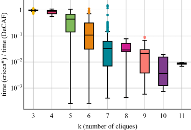
Figure 1. DeCAF improves the runtime of cricca* by two orders of magnitude. We plot the ratio of execution time on all instances that completed in 3600s with both algorithms. Instances are binned by $k$, the number of cliques in the desired decomposition, highlighting that the improvement in runtime increases with the parameter value.

2. Preliminaries

We begin by formally defining EWCD, first introduced by Cooley et al. as a combinatorial model for discovering modules in gene co-expression graphs (Cooley et al., 2021).

To solve this problem, the authors of (Cooley et al., 2021) also introduced a generalization called Annotated EWCD (AEWCD) that allowed some vertices to have positive weights.

Thus, EWCD is the special case of AEWCD when the set $S=\varnothing$. The authors showed that an instance of EWCD can be reduced to an equivalent instance of AEWCD with at most $4^{k}$ vertices (Cooley et al., 2021). Their reduction techniques are based on those of Feldman et al. (Feldmann et al., 2020), who consider a closely related problem Weighted Edge Clique Partition (WECP) and its generalization Annotated WECP (AWECP). WECP is the special case of EWCD when the clique weights are restricted to be $1$. Specifically, for a graph $G$ with edge weights $w_{e}$ and $k\in\mathbb{Z}^{+}$, $(G,k)$ is a YES-instance of WECP iff there is a multiset of at most $k$ cliques such that each edge appears in exactly $w_{e}$ cliques.

Both these works heavily use linear algebraic techniques, and give equivalent matrix problem formulations in which matrices are allowed to have wildcard entries denoted by $\star$. For $a,b\in\mathbb{R}\cup\left\{\star\right\}$, let $a\stackrel{{\scriptstyle\star}}{{=}}b$ if either $a=b$ or $a=\star$ or $b=\star$. For matrices $M1$ and $M2$, we write $M1\stackrel{{\scriptstyle\star}}{{=}}M2$ if $M1_{ij}\stackrel{{\scriptstyle\star}}{{=}}M2_{ij}$ for each $i,j$. The reformulation of AEWCD (given by (Cooley et al., 2021)) is called Binary Symmetric Weighted Decomposition with Diagonal Wildcards (BSWD-DW).

Essentially, the goal is to find an $n\times k$ binary matrix $B$ and a $k\times k$ diagonal matrix with non-negative elements, $W$ such that ${A\stackrel{{\scriptstyle\star}}{{=}}BWB^{T}}$. The matrix $A$ represents the weighted adjacency matrix of $G$ i.e. $A_{i,j}$ represents the weight of the edge $(i,j)$. If edge $(i,j)$ does not exist in $G$, then $A_{i,j}=0$. In the diagonal matrix $W$, each column (and row) represents a clique from the solution and the element $W_{i,i}$ represents the weight of the $i^{th}$ clique. The wildcard entries in $A$ are used for vertices with no weight restrictions. EWCD is thus the special case of BSWD-DW where all the diagonal entries are wildcards.

We say that two distinct vertices $u$ and $v$ in G are $\star$-twins if they are adjacent and satisfy $A_{u}\stackrel{{\scriptstyle\star}}{{=}}A_{v}$ . We partition the vertices of $G$ (and correspondingly the rows of $A$) into sets of vertices called blocks such that vertices $u$ and $v$ belong to the same block iff $u$ and $v$ are $\star$-twins.  (Feldmann et al., 2020) showed that blocks are essentially equivalence classes.

We use $M_{i}$ to represent the $i^{th}$ row of a matrix $M$. The row vector $B_{i}$ represents the membership information of the $i^{th}$ vertex, i.e. $B_{i,j}$ represents whether the vertex $i$ is a member of the $j^{th}$ clique. We call $B_{i}$ the signature of the vertex $i$.

2.1. Related Work

There is a rich history of work emphasizing the importance of mining patterns in gene co-expression analysis  (Xiao et al., 2014; Yan et al., 2007; Visscher et al., 2017; Nelson et al., 2015) in which information about pairwise correlations for all genes in organisms (Mercatelli et al., 2020) is used to derive useful knowledge about sets of genes whose expression is consistently modulated across the same tissues or cell types. Typically, unsupervised network-based learning approaches (Mao et al., 2019; Taroni et al., 2019; de Leeuw et al., 2015) are used for mining such modules. The first combinatorial model of module identification was Exact Weighted Clique Decomposition (EWCD), introduced in (Cooley et al., 2021). They gave a $4^{k}$-kernel and two parameterized algorithms for obtaining the decomposition of a graph into weighted cliques, one based on linear programming (LP) that works for real-valued weights, and an integer partitioning-based algorithm for the restricted case of integral weights. Both algorithms performed comparably so we use the unrestricted LP-based algorithm.

If clique weights are restricted to all being 1, EWCD is equivalent to Weighted Edge Clique Partition (WECP) as studied by  (Feldmann et al., 2020). Their work builds upon the linear algebraic techniques of Chandran et al. (Chandran et al., 2017) for solving the Biclique Partition problem. WECP itself generalizes Edge Clique Partition (ECP) (Ma et al., 1988) which seeks a set of cliques containing each edge at least once (but no constraint on the maximum number of occurrences). It is known that ECP admits a $k^{2}$-kernel in polynomial time (Mujuni and Rosamond, 2008).

On the matrix factorization side, where (Cooley et al., 2021) modeled EWCD as the BSWD-DW problem, several other minimization objectives have been studied. Zhang et al. (Zhang et al., 2013) minimized ${\|A-BB^{T}\|_{2}^{2}}$ and Chen et al. (Chen et al., 2021) considered ${\|A-BB^{T}\|_{0}}$. However, neither of these formulations allow wildcard entries, and hence they are unable to model the clique decomposition problem. The Off-Diagonal Symmetric Non-negative Matrix Factorization Problem studied by Moutier et al. (Moutier et al., 2021) allows diagonal wildcards but also allows $B$ to be any non-negative matrix (not just binary).

3. Main ideas

The starting point for this work is the algorithm of  (Cooley et al., 2021) for EWCD. The algorithm first preprocesses the graph to remove isolated vertices from $G$ and adjusts $k$ accordingly (each isolated vertex must be a unique clique in every valid decomposition). It then uses the kernelization techniques of  (Feldmann et al., 2020) to obtain a smaller equivalent instance of AEWCD. On this kernelized instance, it runs a (parameterized) clique decomposition algorithm that searches the space of clique membership signatures for each vertex. Note that the kernel reduction rules of  (Feldmann et al., 2020) were proposed for the AWECP problem in which clique weights are restricted to be $1$.  (Cooley et al., 2021) showed that the same rules can be used to obtain a kernel for AEWCD. We will follow a similar sequence by first giving a kernel reduction rule for AWECP and then showing that it can also be used for AEWCD. Thus, we first consider the setup of the AWECP problem.

The kernelization technique of  (Feldmann et al., 2020) works by applying two reduction rules to blocks of $\star$-twins which either prune away many of the vertices from the block or act as easy checks for a NO-instance.

Kernel Rule 1 ((Feldmann et al., 2020)).

If there are more than $2^{k}$ blocks, then output that the instance is a NO-instance.

Kernel Rule 2 (informal, (Feldmann et al., 2020)).

If there is a block $D$ of size greater than $2^{k}$, then pick two distinct $i,j\in D$. Convert $G$ into an instance $G^{\prime}$ of AEWCD by setting the weight of vertex $i$ equal to the weight of edge $(i,j)$ and removing every vertex in $D$ from $G$ except $i$. Then $(G,k)$ is a YES-instance iff $(G^{\prime},k)$ is a YES-instance.

For Kernel Rule 1 (K-rule 1), the authors  (Feldmann et al., 2020) show that if $G$ is a YES-instance, then any pair of vertices $u,v$ in $G$ such that $u$ and $v$ have different signatures in the solution must belong to different blocks. Since there can be at most $2^{k}$ possible signatures (binary vectors of length $k$) there can be at most $2^{k}$ blocks in a YES-instance.

For Kernel Rule 2 (K-rule 2), they first prove that if $G$ is a YES-instance then for any block of vertices, there exists a solution in which all the vertices from the block either have the same signature or all have pairwise distinct signatures. Since there can be at most $2^{k}$ distinct signatures, if the number of vertices in a block is greater than $2^{k}$ then by the pigeonhole principle, the signatures cannot all be distinct. Hence, there must exist a solution in which all the vertices in the block have the same signature. In such a case, we can keep just one representative vertex from the block to get a smaller instance.

Note that this means that any two vertices of such a block must participate in exactly the same set of cliques. For this to happen, for vertices $u,v$ in the block, the weight $w$ of the edge $(u,v)$ must equal the number of cliques that contain $u$ and $v$ in the solution. Any solution for the reduced instance that is extendable to a solution for the original instance must ensure that the representative vertex $v$ is part of exactly $w$ cliques. To enforce this condition the weight of the representative vertex is set to $w$ in the reduced instance.

Thus, after applying K-rules 1 and 2 there are at most $2^{k}$ blocks with at most $2^{k}$ vertices in each block. In this way, the authors obtain a kernel of size $4^{k}$. Although this kernel was proposed by  (Feldmann et al., 2020) for WECP in which the clique weights have to all be 1,  (Cooley et al., 2021) showed that the same techniques apply even when the cliques are allowed non-unit weights.

Our main insight is that K-rule 2 applies to a broader set of blocks. Specifically, we show that if $G$ is a YES-instance then for any block with more than $k$ vertices, all vertices of the block must have identical signatures. For this, we use Fisher’s inequality to prove that if a block has $\geq k+1$ vertices and not all vertices of the block participate in the same cliques, then the number of cliques required to cover the edges in the block is at least $k+1$, contradicting the assumption that the given instance is a YES-instance. Thus, we apply K-rule 2 to every block with $\geq k+1$ vertices. Since there are at most $2^{k}$ blocks and each block has at most $k$ vertices, we obtain a $k2^{k}$-kernel. Although this gives a kernel for the WECP problem (in which cliques are constrained to have unit weight), similar to  (Cooley et al., 2021) we show that this works for EWCD as well. The running time of the kernelization algorithm remains unchanged at $O(n^{2}\log n)$. In practice, we observe that this K-rule gives an order of magnitude reduction in the size of the kernel, which subsequently helps speed up the decomposition.

Search Rules (S-rules): The decomposition algorithm of  (Cooley et al., 2021) uses backtracking to assign signatures to vertices one by one. While doing so, it checks to make sure that the new signature is compatible with the vertices that have already been assigned a signature. If no compatible signature is found for a vertex, the algorithm backtracks. It continues this process until all vertices have a valid assignment or it determines that no valid assignment can be found. Having rules that can quickly detect that the current (partial) assignment cannot be extended to a valid decomposition helps us prune away branches of the search tree and reduce the running time.

Our first S-rule pertains the order in which we consider the vertices for signature assignment, which can significantly affect how much of the search tree must be explored. We tested several strategies, and found that a push_front approach in which vertices from reduced blocks are considered before those in non-reduced blocks was most effective. A justification for this strategy is in Section 5, and the empirical evaluation is shown in Section 6.2.

Our second S-rule comes from the straightforward observation that when assigning a signature to a vertex, one must respect its non-neighbor relationships. More specifically, when finding a signature for a vertex $v$, for all $u$ such that $(u,v)$ is not an edge, $B_{u}B_{v}^{T}=0$. That is, if $u$ and $v$ are non-neighbors, they cannot share a clique. Thus, we only test those signatures for $v$ that have no cliques in common with the signatures of its non-neighbors.

Our third and final S-rule makes use of the fact that if the graph is a YES-instance then there exists a solution in which all vertices in each block have either identical signatures or pairwise distinct signatures. Thus, when assigning signatures to the vertices of a block, either we assign a unique signature to all vertices in the block or assign the same signature to all vertices in the block. This eliminates assignments in which a block has the same signature appearing on more than $1$ but but not all vertices in the block.

The improved kernel along with these S-rules speeds up decomposition by two orders of magnitude. We give formal proofs of our results in the next two sections.

4. Smaller kernel

Similar to  (Cooley et al., 2021), we will first consider the setup of the AWECP problem (in which the cliques are constrained to have weight 1), and prove correctness of our new reduction rule. We will then show that the rule remains valid in the case of AEWCD. We begin by restating an important lemma from (Feldmann et al., 2020).

Lemma 4.1 (Restated Lemma 8 from  (Feldmann et al., 2020)).

For a block $D$, the entries of the sub-matrix $A_{D,D}$ are all same except for wildcards.

An important property of $\star$-twins implied by Lemma 4.1 is: if vertices $u$ and $v$ are $\star$-twins and $u$ is annotated, then $A_{uu}=A_{uv}$. In other words, the weight of $u$ must equal the weight of the edge $(u,v)$ because otherwise $A_{uv}$ is not $\stackrel{{\scriptstyle\star}}{{=}}$ to $A_{vv}$, contradicting the fact that $u$ and $v$ are $\star$-twins. Any block (definitionally) consists exclusively of $\star$-twins, thus, the weight of every edge within the block must be the same. In other words, the vertices in the block form a complete subgraph with uniform edge-weights.

An important observation about any solution for WECP (EWCD) is that since the vertices do not have weights, if the solution contains a singleton clique (i.e. a clique of size 1) and if we remove this clique the remaining set of cliques also forms a solution. (Recall that isolated vertices have already been removed in the preprocessing step). Thus, in the rest of this paper, we restrict our attention to solutions that do not contain singleton cliques. Note that, on the other hand an instance of AWECP (AEWCD) obtained from an instance of WECP (EWCD) can have singleton cliques to satisfy vertex weights. However, such vertices must necessarily be the representative vertices of reduced blocks.

We now formally define two types of $\star$-twins.

Definition 4.2 (Identical and fraternal twins).

Given a YES-instance $(G,k)$ of AWECP, $\star$-twins $u$ and $v$ in $G$ are called identical twins if there exists no solution in which $u$ and $v$ have distinct signatures, and fraternal twins otherwise.

Note that there can be solutions in which fraternal twins have identical signatures – we only require that in some solution they have different ones. Moreover, since a block consists of $\star$-twins, if any two vertices in a block are identical twins, then all must be. We call such blocks identical blocks.

K-rule 2 from  (Feldmann et al., 2020) implies that all blocks with $>2^{k}$ vertices are identical blocks. Our main insight is that a broader set of blocks must have this property. More specifically, any block with $>k$ vertices must be an identical block.

To prove this, we will use a result from combinatorial design theory known as the non-uniform Fisher’s inequality:

Theorem 4.3 (restated from  (Mathew and Mishra, 2020)).

Let $w$ be a positive integer and let $A=\{A_{1},...,A_{t}\}$ be a family of subsets of $U=\{e_{1},...,e_{r}\}$. If $|A_{i}\cap A_{j}|=w$ for each $1\leq i<j\leq t$, then $|A|=t\leq r=|U|$.

Essentially, the non-uniform Fisher’s inequality states that if we have a set of $r$ elements and we form $t$ subsets of these elements such that any two subsets intersect in exactly $w$ elements, then the number of subsets can be at most the number of elements.

Fisher’s inequality was first proposed in the context of Balanced Incomplete Block Design (BIBD) (See  (Stinson, 2004) and  (Babai and Frankl, 1988)). The uniform version was first proposed by Ronald Fisher and Majumdar (Majumdar, 1953) showed that the inequality holds even in the non-uniform case. The inequality has since been proven and applied in many different problem areas. In fact, De Caen and Gregory  (de Caen and Gregory, 1985) showed the following corollary which, as we will show below, directly corresponds to the problem we’re considering.

Let $K_{t}$ represent the unweighted, complete graph on $t$ vertices, and $wK_{t}$ denote the complete multigraph on $t$ vertices where the multiplicity of every edge is $w$. Let us say that a partition $R$ of the edge-set of $wK_{t}$ into cliques is non-trivial if there exists any clique in $R$ that is not $K_{t}$. Corollary 4.4 implies if $R$ is non-trivial then $t\leq|R|$. This can also be viewed as a generalization of the clique partition theorem of De Bruijn and Erdös  (de Bruijn and Erdös, 1948) for arbitrary $w$ (the result of  (de Bruijn and Erdös, 1948) was for $w=1$).

Corollary 4.4 (restated Corollary 1.4 from  (de Caen and Gregory, 1985)).

Let $R$ be a partition of the edge-set of $wK_{t}$ into non-empty cliques. If not all cliques in $R$ are $K_{t}$ then $|R|\geq t$.

We are now ready to prove our main theorem. Let $D$ be a block with $t=|D|\geq k+1$ vertices. Let $w$ be the weight of the edges in $D$.

Theorem 4.5.

If the given instance $(G,k)$ is a YES-instance of AWECP, then $D$ must be an identical block.

Proof.

Suppose $D$ is not identical. Since $G$ is a YES-instance, there exists a solution such that not all vertices from $D$ have the same signature i.e. not all vertices from $D$ appear in the same cliques. Let $S$ be the multiset of cliques in such a solution. Let $S_{D}\subseteq S$ be the multiset of cliques in which vertices from $D$ appear. From every clique $C\in S_{D}$, delete all vertices that are not in $D$ and call the resultant multiset $R$. Thus, $R$ is a multiset of subsets of $D$. Since any subset of vertices in a clique also form a (smaller) complete graph, $R$ is a multiset of cliques. One can think of the cliques in $R$ as the “projection” of the cliques in $S_{D}$ onto $D$. Since, not all vertices from $D$ appear in the same cliques, $R$ must consist of a non-trivial clique.

We first show that the non-trivial cliques in $R$ cannot all be singleton cliques. Suppose there is a singleton clique in $R$ consisting of $v\in D$. Then there exists a non-singleton clique $C$ in $S_{D}$ such that $C\cap D=v$. Moreover, since $C$ is not singleton, there exists a vertex $v^{\prime}\in C\setminus D$. Let $u\neq v$ be a vertex in $D$. Since $u$ and $v$ are $\star$-twins and $v$ is a neighbor of $v^{\prime}$, $u$ must also be a neighbor of $v^{\prime}$ and $w_{uv^{\prime}}=w_{vv^{\prime}}$. Thus, there must exist a clique $C^{\prime}\in S_{D}$, $u,v^{\prime}\in C^{\prime},v\notin C^{\prime}$. In other words, every vertex $u\in D,u\neq v$ must be a part of some clique that $v$ is not a part of. If each such clique projects into a singleton clique in $R$, then $|R|>|D|=k+1$ which is a contradiction since $G$ is a YES-instance. Thus, there must exist a non-singleton, non-trivial clique in $R$ i.e. there must exist a clique containing $>1$ but not all vertices from $D$.

Let $H$ be an unweighted, complete multigraph on $|D|$ vertices in which the multiplicity of every edge is $w$. It is easy to see that $R$ is a partition of the edge-set of the multigraph $H$ into cliques. If $R$ consists of a non-singleton, non-trivial clique then by  Corollary 4.4, $|D|\leq|R|$, which is a contradiction because $G$ is a YES-instance (implying $|R|\leq k$ and $|D|\geq k+1$). Thus, $R$ cannot consist of non-trivial cliques.

In other words, $R$ must be trivial i.e. every clique in $R$ must be a $K_{t}$. Thus, every vertex of $D$ must be in the exact same set of cliques in $S$ and have the same signature in the solution matrix $B$. Thus, $D$ must be an identical block.

∎

Hence, we can reduce it to a representative vertex, leading to our enhancement of K-rule 2:

Kernel Rule 2+.

If there is a block $D$ of size greater than $k$, then apply the reduction of K-rule 2.

We further show that K-rule 2+ gives a valid kernel even in the case of AEWCD. Our proof of correctness closely follows that of rule 2 in  (Cooley et al., 2021) and proceeds in two parts. Proofs of these Lemmas are deferred to Appendix A.2.

Lemma 4.6.

Let $(A^{\prime},k)$ be the reduced instance constructed by applying K-rule 2+ to $(A,k)$. Then if $(B^{\prime},W^{\prime})$ is a solution for $(A^{\prime},k)$ then the $(B,W)$ constructed by 2+ is indeed a solution to $(A,k)$.

Lemma 4.7.

If $(A,k)$ is a YES-instance, then the reduced instance $(A^{\prime},k)$ produced by 2+ is a YES-instance.

Thus, our kernelization algorithm applies K-rule 1 of  (Cooley et al., 2021) and K-rule 2+ to get a kernel that is at most $k2^{k}$ in size. The kernelization algorithm sorts the rows in $A$ to form blocks and reduces each block that has $\geq k+1$ vertices. The sorting of rows of $A$ and division into blocks takes time $O(n^{3})$ and the application of K-rule 1 and K-rule 2+ take time $O(n)$. Thus, the time complexity of the kernelization algorithm is $O(n^{3})$, matching that of  (Cooley et al., 2021).

5. Faster Decomposition Algorithm

Once a kernelized instance is obtained, one can run the decomposition algorithm of  (Cooley et al., 2021), shown in CliqueDecomp-LP (Algorithm 1), on it. The algorithm assigns signatures to vertices one-by-one, iteratively building a solution. When only a subset of all vertices have been assigned a signature, we call this a partial assignment. When trying to find a compatible signature for a vertex, the algorithm searches the entire space of $2^{k}$ possible signatures for that vertex. For every signature that the algorithm considers for a vertex, the clique weights as given by the weight matrix $W$ may need to change. iWCompatible (Algorithm 3) checks if the weight matrix $W$ is compatible with the current partial assignment. If not, to find a compatible new set of weights, the algorithm builds a Linear Program (LP) which encodes the partial assignment and the edge-weights (InferCliqWts-LP, Algorithm 4). If the LP returns a solution, the algorithm updates the weight matrix. If the LP fails to return a solution, it means that no feasible weight matrix exists for this partial assignment. In this case, the algorithm backtracks. Since InferCliqWts-LP and iWCompatible are not affected by our search reduction rules, we defer their pseudocode to the appendix.

1:for $P\in\{0,1\}^{2k\times k}$ do

2:     initialize $\widetilde{B}$ to a $n\times k$ null matrix

3:     $b,i\leftarrow 1$

4:     while $b\leq 2k$  do

5:         $\widetilde{B}_{i}\leftarrow P_{b}$

6:         $b\leftarrow b+1$

7:         $W\leftarrow$ InferCliqWts-LP ($A$, $\widetilde{B}$)

8:         if $W$ is not null matrix then

9:              $(B,i)\leftarrow$ FillNonBasis (A, $\widetilde{B}$, $W$)

10:              if $i=n+1$ then return ($B$, $W$)               

11:         else$\;b\leftarrow 2k+1$ $\triangleright$ null $W$; break out of while               

12:return No

Algorithm 1 . CliqueDecomp-LP

The main insight of  (Cooley et al., 2021) was that the pseudo-rank of $B$ is at most $2k$ and that once the basis vectors of $B$ have been guessed correctly, there will be no need to backtrack when filling in the signatures of other vertices. They showed that we need to run the LP only when the algorithm backtracks and that this happens for at most $2^{2k^{2}}$ partial assignments. FillNonBasis (Algorithm 2) shows the pseudocode for filling in the signatures for the non-basis vectors. Note that every time the algorithm picks a new set of basis vectors ($P$), the existing assignment of signatures (even non-basis vectors) are discarded. After an exhaustive search if no valid assignment is found, the algorithm returns that the instance is a NO-instance.

1:$B\leftarrow\widetilde{B}$

2:while $B$ has a null row do

3:     let $B_{i}$ be the first null row

4:     for $v\in\left\{0,1\right\}^{k}$ do

5:         if iWCompatible ($A$, $B$, $W$, $i$, $v$) then

6:              $B_{i}\leftarrow v$

7:              goto line 2               

8:     return $(B,i)$ $\triangleright$ there is no $(i,W)$-compatible $v$

9:return $(B,n+1)$ $\triangleright$ B has no null row

Algorithm 2 . FillNonBasis ($A$, $\widetilde{B}$, $W$)

We now design several search reduction rules that can help to quickly prune away branches that cannot lead to a solution.

Search Rule 0: Assign signatures to reduced blocks before non-reduced blocks. We observed during experiments that the order in which we assign signatures to vertices can significantly impact how fast the algorithm terminates. Ideally, we would like the first $k$ vertices to be as close to an independent set as possible (since non-neighbors significantly restrict potential valid signatures, see S-rule 1). Since vertices within a block must be neighbors, we wanted an order that hit many distinct blocks quickly, yet was compatible with the engineering required for S-rule 2 (below). This led to the strategy push_front, which assigns signatures to all vertices which are representatives of reduced blocks (which necessarily have size 1) before proceeding to those in non-reduced blocks. We validated our choice by empirically evaluating this against several other orders including the arbitrary approach in  (Cooley et al., 2021); details are in  Section 6.2.

Search Rule 1: For every vertex, generate only those signatures that don’t share a clique with the non-neighbors of that vertex. The main idea behind S-rule 1 is that any two non-neighbors should not share a clique. Thus, for non-neighbors $u$ and $v$, $B_{u}{B_{v}}^{T}=0$. Whenever the algorithm is searching for a signature to assign to a new vertex, it generates the list of cliques that are “forbidden” for that vertex based on the signatures of the vertex’s non-neighbors. It then uses this list to generate only those signatures that respect the “forbidden” cliques. In many cases, this drastically reduces the number of signatures to be tried.

Search Rule 2: Vertices across blocks must have unique signatures. The cliques that a vertex participates in cannot be a proper subset of the cliques its $\star$-twin participates in. Make all signatures in a block either identical or pairwise distinct.

We first prove that signatures cannot be shared across blocks.

Lemma 5.1.

If $u$ and $v$ belong to different blocks then $B_{u}\neq B_{v}$.

Proof.

For contradiction, assume $B_{u}=B_{v}$. Since $u$ and $v$ belong to different blocks, they must not be $\star$-twins. Thus, either $u$ is not adjacent to $v$ or $A_{u}\stackrel{{\scriptstyle\star}}{{\neq}}A_{v}$.

If $u$ is not adjacent to $v$, $A_{uv}=B_{u}WB_{v}^{T}=0$. Since, $B_{u}=B_{v}$ and since we do not allow cliques to have weight $0$, $B_{u}WB_{v}^{T}=0$ iff $B_{u}=B_{v}=0$. Thus, it must be the case that $B_{u}=B_{v}=0$. However, since the graph has already been preprocessed to remove all isolated vertices, the remaining vertices must all have at least one edge adjacent to them and hence must be a part of at least one clique. Thus, $B_{u},B_{v}\neq 0$ which is a contradiction.

Now consider the case when $u$ and $v$ are adjacent but $A_{u}\stackrel{{\scriptstyle\star}}{{\neq}}A_{v}$. Since $B_{u}=B_{v}$, $B_{u}WB^{T}=B_{v}WB^{T}$. Since $B_{u}WB^{T}\stackrel{{\scriptstyle\star}}{{=}}A_{u}$ and $B_{v}WB^{T}\stackrel{{\scriptstyle\star}}{{=}}A_{v}$, this implies that $A_{u}\stackrel{{\scriptstyle\star}}{{=}}A_{v}$, a contradiction. ∎

We will now show that there cannot be $\star$-twins such that the signature of one is a subset of the signature of the other. Note that when we apply the S-rules, the graph has already been preprocessed. Thus, there are no isolated vertices in $G$.

Lemma 5.2.

Consider a YES-instance $(G,k)$ of AEWCD. There exists a solution $B$ such that for every pair of vertices $u$ and $v$ that are $\star$-twins in $G$, $B_{u}\nsubset B_{v}$ and vice versa.

Proof.

Suppose there exist $\star$-twins $u$ and $v$ and a solution $B$ such that $B_{u}\subset B_{v}$. Then there exists a clique $C$ in the solution such that $v\in C,u\notin C$. If $C$ is a singleton clique or $C$ has weight $0$, then we can remove $C$ from the solution. Clearly, the remaining set of cliques would still be a solution and the theorem would be true. So assume $C$ has positive weight and is not a singleton clique. Thus, there exists a vertex $v^{\prime}\in C,v^{\prime}\neq v$. Since $u$ and $v$ are $\star$-twins and $v$ is a neighbor of $v^{\prime}$, $u$ must also be a neighbor of $v^{\prime}$ and $w_{uv^{\prime}}=w_{vv^{\prime}}$. Let $S_{uv^{\prime}}$ and $S_{vv^{\prime}}$ be the set of cliques in the solution in which edges $(u,v^{\prime})$ and $(v,v^{\prime})$ participate, respectively. Then since $B_{u}\subset B_{v}$, $S_{uv^{\prime}}\subset S_{vv^{\prime}}$. Moreover, $w_{uv^{\prime}}=\sum_{i:{uv^{\prime}}\in C_{i}}\gamma_{i}$ where $\gamma_{i}$ represents the weight of clique $i$. Similarly, $w_{vv^{\prime}}=\sum_{i:{vv^{\prime}}\in C_{i}}\gamma_{i}$. But since the cliques have positive weights and $S_{uv^{\prime}}\subset S_{vv^{\prime}},w_{uv^{\prime}}<w_{vv^{\prime}}$ which is a contradiction. ∎

We know from Theorem 4.5 that blocks having $>k$ vertices must be identical blocks. However, blocks having $\leq k$ vertices can be fraternal. Moreover, by Lemma 11 of  (Feldmann et al., 2020) we know that if the given instance is a YES-instance then there exists a solution in which all vertices in a block have either identical signatures or pairwise distinct signatures. We show that if the given instance is a YES-instance of AEWCD then there exists a solution in which this condition is simultaneously true for all blocks.

Theorem 5.3.

Given a YES-instance $(G,k)$ of AEWCD, there exists a solution in which every block of $G$ has either identical signatures or pairwise distinct signatures.

Proof.

Consider any solution $(B,W)$ to the given instance and suppose there exists a block $D$ whose vertices have signatures that are neither all unique nor all pairwise-disjoint (if such a block does not exist then the theorem is trivially true). Thus, there exist vertices $v_{1},v_{2},v_{3}$ in $D$ such that $B_{v_{1}}=B_{v_{2}}\neq B_{v_{3}}$. Consider the $n\times k$ matrix $B^{\prime}$ got by setting ${B^{\prime}}_{v_{1}}=B_{v_{1}}$, ${B^{\prime}}_{v_{2}}=B_{v_{2}}$, ${B^{\prime}}_{v_{3}}=B_{v_{1}}$ and $\forall x\neq v_{1},v_{2},v_{3},{B^{\prime}}_{x}=B_{x}$ i.e. $B^{\prime}$ has the same signatures as $B$ for all vertices except $v_{3}$ and ${B^{\prime}}_{v_{3}}$ is set to $B_{v_{1}}$. To prove that $(B^{\prime},W)$ is indeed a valid solution for $(G,k)$, it is sufficient to show that ${B^{\prime}_{u}}W{B^{\prime}}_{v}^{T}\stackrel{{\scriptstyle\star}}{{=}}A_{uv}$ for all vertices $u,v$ in $G$. There are 3 cases to consider:

• Case 1: $u,v\neq v_{3}$. Then ${B^{\prime}_{u}}W{B^{\prime}}_{v}^{T}={B_{u}}W{B_{v}^{T}}\stackrel{{\scriptstyle\star}}{{=}}A_{uv}$.

• Case 2: $u=v_{3}$,$v\neq v_{3}$. Then ${B^{\prime}_{u}}WB_{v}^{T}={B_{v_{1}}}WB_{v}^{T}\stackrel{{\scriptstyle\star}}{{=}}A_{v_{1}v}=A_{v_{3}v}$, where the last equality follows from $v_{1}$ and $v_{3}$ being in the same block $D$.

• Case 3: $u=v=v_{3}$. In this case, ${{B^{\prime}}_{v_{3}}}W{B^{\prime}}_{v_{3}}^{T}={B_{v_{1}}}WB_{v_{3}}^{T}\stackrel{{\scriptstyle\star}}{{=}}A_{v_{1}v_{3}}\stackrel{{\scriptstyle\star}}{{=}}A_{v_{3}v_{3}}$. The $\stackrel{{\scriptstyle\star}}{{=}}$ here follows because any two entries (that are not $\star$) in the same block of matrix $A$ are equal (Lemma 7 of (Feldmann et al., 2020)).

We can apply this iteratively to all vertices in $D$ and to other blocks until all blocks either have identical signatures or pairwise distinct signatures. ∎

Thus, we only need to search over those assignments that satisfy the conditions of Theorem 5.3. In 5 in CliqueDecomp-LP and 4 in FillNonBasis, when assigning a signature to a vertex we ensure that all vertices in its block have either identical or unique signatures. This eliminates assignments in which a block consists of some repeated signature but not all identical signatures, thereby reducing the search space.

Running time: The for loop in 1 has at most $2^{{2k}^{2}}$ iterations. FillNonBasis takes time $O(n^{2}k2^{k})$ where $n$ is the number of vertices in the kernelized instance. InferCliqWts-LP solves an LP with $k$ variables and at most $4k^{2}$ constraints which can be solved in $O(k^{4}L)$ time where $L$ is the number of bits required for input representation (Vaidya, 1989). iWCompatible runs in time $O(nk)$ and hence, the total time taken by FillNonBasis is $O(n^{2}k2^{k})$. Hence, the total time taken by CliqueDecomp-LP without the S-rules is $O(2^{{2k}^{2}}2k(k^{4}L+n^{2}k2^{k}))$. Since $n\leq 4^{k}$ the total running time of CliqueDecomp-LP as given by  (Cooley et al., 2021) is $O(4^{k^{2}}k^{2}(32^{k}+k^{3}L))$. Thus, if $L=O(2^{k})$, this comes to $O(4^{k^{2}}k^{2}32^{k})$.

S-rule 0 pushes singleton vertices from reduced blocks to front in time $O(n)$. S-rule 1 when assigning a signature to a vertex $v$, loops over the non-neighbors of $v$ and generates the list of forbidden cliques in time $O(nk)$. S-rule 2 when assigning a signature to a vertex, compares with the signatures of other vertices in the block in $O(nk)$ time. Thus, the running time of CliqueDecomp-LP with S-rules is $O(2^{{2k}^{2}}2nk^{2}(k^{4}L+n^{2}k2^{k}))$ Due to the new kernel, we can set $n=k2^{k}$. This gives an overall running time of $O(4^{k^{2}}2^{k}k^{4}(k^{2}2^{3k}+k^{3}L))$. Thus, if $L=O(2^{k})$ this comes to $O(4^{k^{2}}k^{6}16^{k})$. Thus, the running time reduces significantly and in practice we are able to get at least two orders of magnitude speedup.

6. Experimental Results

We compared the performance of our kernelization and decomposition algorithms with those of  (Cooley et al., 2021). We use the publicly available Python package of  (Cooley et al., 2021) provided by its authors and implement our new algorithms as an extension. We ran all experiments on identical hardware, equipped with 40 CPUs (Intel(R) Xeon(R) Gold 6230 CPU @ 2.10GHz) and 191000 MB of memory, and running CentOS Linux release 7.9.2009. We used Gurobi Optimizer 9.1.2 as the LP solver, parallelized using 40 threads. A timeout of 3600 seconds per instance was used in all experiments. Code and data to replicate all experiments are available at (Anon., [n. d.]), and will be made open-source before publication.

Notation: We use $K_{D}$ and $S_{D}$ to denote our kernelization and decomposition algorithms, respectively. We use $K_{C}$ to denote the kernelization algorithm of  (Cooley et al., 2021), and $S_{C}$ ($S_{C^{*}}$) for the decomposition algorithm of  (Cooley et al., 2021) without (with) S-rule 0. Thus, cricca represents the combination ($K_{C}$, $S_{C}$), cricca* is ($K_{C}$, $S_{C^{*}}$) and DeCAF is($K_{D}$, $S_{D}$). We use $n_{C}$ and $n_{D}$ to denote number of vertices remaining in the graph (the kernel) after applying $K_{C}$ and $K_{D}$ respectively. For some of our experiments, we subselect instances based on their seed. Details can be found in the description of each experiment.

Datasets: The authors of  (Cooley et al., 2021) evaluate cricca on two biology-inspired synthetic datasets (LV and TF, seeds 0-19); we use the same datasets for our experiments. Details about how these datasets were created are in Section 7 and Appendix D of (Cooley et al., 2021). We assume that every graph has been preprocessed to remove isolated vertices. Each (preprocessed) graph $G$ has a ground-truth $k$ – the minimum $k$ such that $(G,k)$ is a YES-instance. We distinguish this from $k_{in}$, which denotes the number of desired cliques input to the algorithms; each $(G,k_{in})$ denotes a unique instance of EWCD. Details about these instances can be found in Table 1. As in (Cooley et al., 2021), we restrict our main corpus to graphs with $3\leq k\leq 11$; for $k\in[5,7]$, we generated multiple instances for each $G$ using several values of $k_{in}$ above and below $k$ (E.3 in (Cooley et al., 2021)). The number of unique $G$ are shown in column “$\#G$” and the number of $(G,k_{in})$ instances are shown in the column “$\#(G,k_{in})$”. The columns $n$ and $m$ denote the average number of vertices and edges across all instances per $k$ value. For ease of comparison of running times, we do not include instances that timed out on any combination of $K_{C}$, $K_{D}$, $S_{C^{*}}$ and $S_{D}$ in Table 1. A detailed breakdown of timeouts is in the Appendix (Section 6.3).

$K_{C}$ $K_{D}$ $S_{C^{*}}$ $S_{D}$ $S_{C^{*}}$ $S_{D}$ cricca* DeCAF $k$ $\#G$ $\#(G,k_{in})$ $n$ $m$ speedup 3 321 321 198.21 38.72 1.00 2.40 2.23 2.45 4 225 225 223.13 146.69 1.00 3.60 4.74 8.81 5 300 564 313.85 2677.86 1.00 6.30 147.91 669.55 6 360 734 369.28 10182.26 1.00 11.83 158.88 1379.24 7 136 274 542.28 28477.22 1.00 13.06 500.44 6061.28 8 31 31 459.77 22834.32 1.00 17.79 169.95 3421.30 9 27 27 824.78 61877.89 1.00 6.45 317.75 9316.60 10 24 24 778.25 116381.50 1.00 22.96 134.39 6876.59 11 18 18 953.00 99219.67 1.00 12.66 128.11 13475.95

Table 1. Corpus number of instances and average sizes grouped by $k$ value (seeds $[0,9]$ and $k\in[3,11]$). Right columns show average runtime reduction for combinations of kernels $K_{C}$, $K_{D}$ and decomposition algorithms $S_{C^{*}}$, $S_{D}$.

6.1. Smaller Kernel

To evaluate the effect of Kernel Rule 2+, we compared the kernel size and the running time of $K_{D}$ with those of $K_{C}$. We used the entire dataset (seeds 0-19) of ground-truth $k$ between $3$ and $11$ (inclusive), with input $k$ ($k_{\text{in}}$) varied between $0.4k$ and $1.6k$. Because the difference between two versions is only the threshold value used in K-rule 2 and K-rule 2+, it holds that $n_{D}\leq n_{C}$. Further, if $K_{C}$ solves the problem, that is, it finds the instance a NO-instance, then so does $K_{D}$.

Figure 2 plots the ratio $n_{D}/n_{C}$ for each instance, colored by $k_{\text{in}}$. We can see that most instances got shrunk to less than 20% of $n_{C}$. Also we observe that our kernel size, $n_{D}$ decreases (1) as $n$ increases and (2) as $k_{\text{in}}$ increases. The former is intuitive; K-rule 2+ is more effective when the instance is larger, removing more vertices from the graph. The latter is explained by the fact that $K_{C}$ is effective only for blocks that are exponential in size with respect to $k_{\text{in}}$ and thus, has less impact when $k_{\text{in}}$ is large, where as $K_{D}$ is able to reduce all blocks with $>k_{in}$ vertices and hence is effective even when $k_{in}$ is large.

For the running time of the kernelization process, we computed the relative running time i.e. the ratio of the running time of $K_{D}$ to that of $K_{C}$. The first and third quantiles were $0.99$ and $1.01$, respectively, and the maximum was $1.24$. We conclude that there is no significant difference in running times.

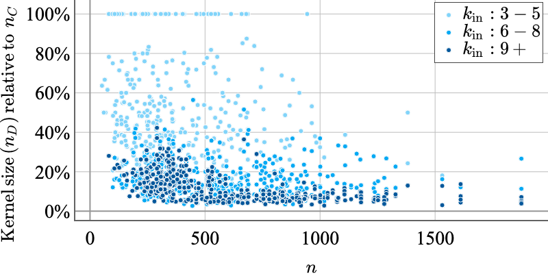
Figure 2. Kernel size of $K_{D}$ relative to that of $K_{C}$ on entire corpus (seeds 0-19), sorted by instance size (prior to kernelization) and colored by $k_{i}n$.

6.2. Effects of Vertex Reordering

We found that vertex ordering has a significant impact on the efficiency of the decomposition process, especially when we obtain a smaller kernel. We experimented with the following orderings.

arbitrary is the baseline strategy used in cricca. It keeps one arbitrary vertex from each block that is reduced and does not reorder the vertices. push_front is the one adopted as S-rule 0. It keeps one arbitrary vertex from each block that is reduced and moves the representative vertex to the front of the ordering. push_back does the opposite; it keeps one arbitrary vertex from each block that is reduced and moves the representative vertex to the back. keep_first keeps the earliest vertex from each block that is reduced and does not reorder the vertices.

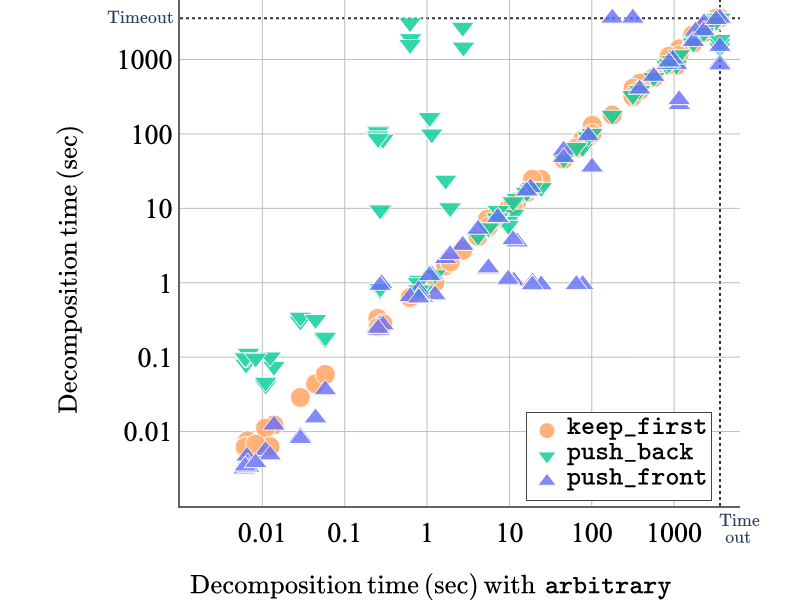
Figure 6. Log-scale plot of decomposition running time distribution with different vertex reordering strategies compared to arbitrary. Tested with the instances of seed 0, $k\in[3,11]$ and the original kernels ($K_{C}$).

To clearly distinguish the effect of ordering (S-rule 0) from the other S-rules, we ran $S_{C^{*}}$ ($S_{C}$ with S-rule 0) on seed 0 instances, where we experimented with each of the above orderings. We obtained results for both $K_{D}$ and $K_{C}$. Figure 3 plots the log-scale distribution of running time of ($K_{D}$, $S_{C^{*}}$) for the different ordering strategies compared to arbitrary. push_front gave the most speedup (10 to 100 times) and did not timeout on any instances. We believe this is because singleton vertices from reduced blocks tend to be non-neighbors which helps to quickly detect infeasible assignments. We observed similar behavior with the ($K_{C}$, $S_{C^{*}}$) combination as shown in Figure 6 in the Appendix.

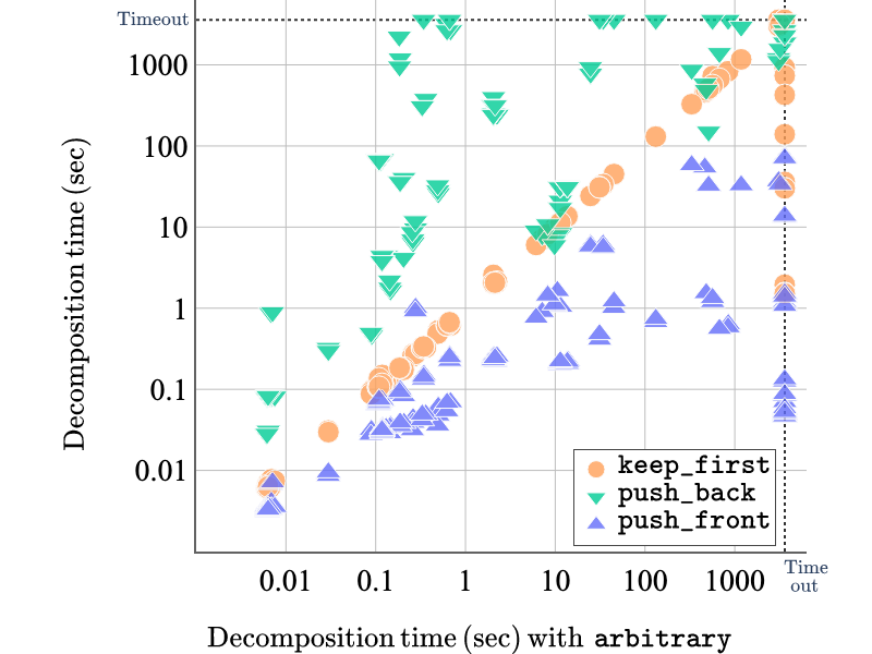
Figure 3. Log-log plot of decomposition runtime distribution on instances with seed 0 using different vertex reordering strategies (and kernel $K_{D}$). Times relative to arbitrary.

6.3. Faster Decomposition

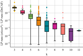
Figure 4. DeCAF reduces the number of LP runs of cricca* by two orders of magnitude. We plot the ratio of number of LP runs on all instances that completed in 3600s with both algorithms. Instances are binned by $k$, the number of cliques in the desired decomposition, highlighting that the reduction in LP runs increases with the parameter value.

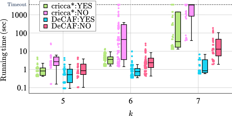
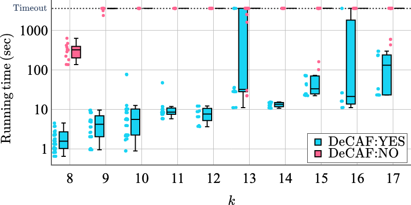
Figure 5. Runtime distribution (log-scale) for cricca* and DeCAF on corpus of YES ($k_{\text{in}}=k$) and NO ($k_{\text{in}}=\lceil 0.8k\rceil$) instances with seeds $[0,9]$ and $5\leq k\leq 7$ (left), and DeCAF only on $8\leq k\leq 17$ (right).

We show results comparing the time taken by cricca* and the time taken by DeCAF for decomposing all instances reported in Table 1. We also do an ablation study and report the effect of the smaller kernel on the running time, with and without search rules.

Comparison with cricca*: Fig. 1 gives the ratio of the running time of cricca* and the running time of DeCAF for different $k$ (lower is better). This includes the kernelization time as well as the time required for decomposition. For small $k$, we do not see a significant reduction in runtime but for larger $k$ we are able to obtain upto two orders of magnitude reduction in the running time, and the trend indicates that the reduction in runtime increases with $k$. Note that we do not include here information about instances for which either cricca* or DeCAF timeout. In the entire corpus of 2556 instances, 297 instances timed out for cricca* and 3 for DeCAF. More detailed information about these instances is in the Appendix (Table 2). Note that the order in which the algorithm considers vertices to assign signatures to impacts the running time. In some cases, despite the smaller kernel and push_front ordering, the running time can go up in the case of DeCAF. Such instances have a ratio $>1$ in Fig. 1 and extremely rare.

Fig. 4 shows the ratio of the number of times the LP solver was invoked by cricca* and the number of times the LP solver was invoked by DeCAF. Because of the search rules and the smaller kernel, we are able to obtain upto three orders of magnitude reduction in the number of runs of the LP solver. Similar to running time, we see an increasing trend in the reduction in the search space with $k$.

Ablation study: To study the relative impact of the smaller kernel and the search rules on the running time of the decomposition algorithm, we tested all four combinations of the kernels ($K_{C}$ and $K_{D}$) and decomposition algorithms ($S_{C^{*}}$ and $S_{D}$). Here, we only consider the running time of the decomposition algorithms and not the kernelization algorithms and do not include numbers for any instance that timed out across all four combinations. Table 1 shows the average reduction obtained in all 4 combinations for different $k$. The smaller kernel has a greater impact on the runtime compared to that of the search rules. Moreover, as expected, the average reduction increases as $k$ increases.

6.4. Scalability

Finally, we evaluate the overall scalability of our implementation. In this section, we consider two input k-values, (1) $k_{\text{in}}=k$ for YES instances and (2) $k_{\text{input}}=\lceil 0.8k\rceil$ for NO instances. In the left figure in Figure 5, we compare four configurations, the combinations cricca*, DeCAF and two $k_{\text{in}}$ values for $k\in[5,6,7]$ with the instances of seeds $[0,9]$. We observe that NO instances take longer than YES instances in both versions. For cricca*, the median runtime reaches the time limit (3600 seconds) with $k=7$ for NO instances. In contrast, DeCAF achieves a median of 13 seconds. For YES instances, for $k=7$ there is an order of magnitude difference in the runtimes of the two algorithms.

To test for scalability, we ran DeCAF on 12 randomly-selected instances for each $k\in[8,17]$. The right figure in Figure 5 shows the distribution of running time for the YES and NO instances. The median runtime for NO instances with DeCAF hits the time limit at $k=9$. Compare this with time taken by cricca* in the left figure of Figure 5; it already hits the time limit at $k=7$. Since both cricca* and DeCAF timeout for $k\geq 9$, we focus on the YES instances.

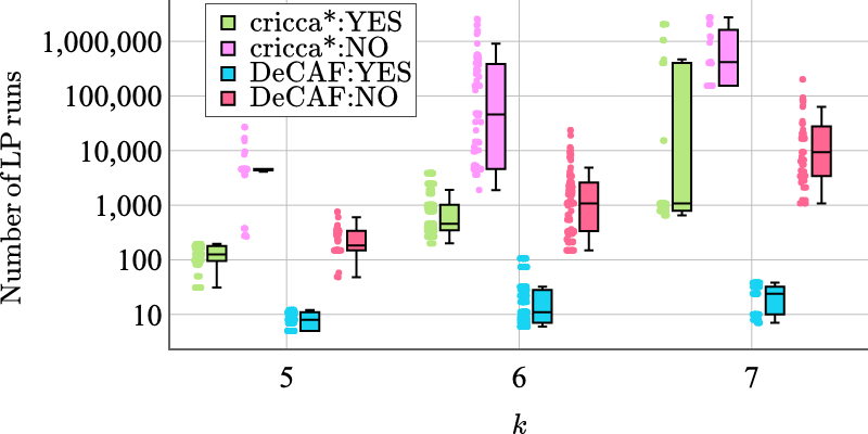
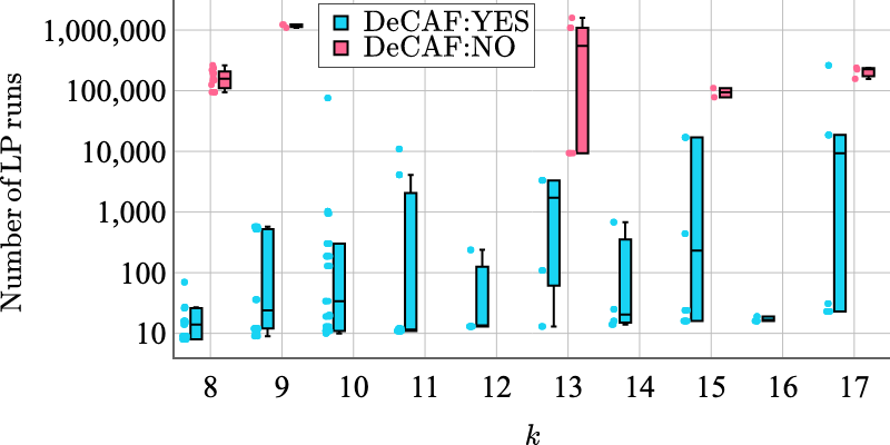
Figure 7. Distribution of number of LP runs (log-scale) for cricca* and DeCAF on corpus of YES ($k_{\text{in}}=k$) and NO ($k_{\text{in}}=\lceil 0.8k\rceil$) instances with seeds $[0,9]$ and $5\leq k\leq 7$ (left), and DeCAF only on $8\leq k\leq 17$ (right).

For YES instances, DeCAF finished within 1000 seconds for all $k$ except for a few “hard” instances with $k=13,16$ (This may happen because the worst-case running time is not polynomially bounded). Compare this with Figure 7 in  (Cooley et al., 2021) which shows that cricca already hits the time limit at $k=9$. We conclude that with DeCAF we are able to scale to at least $1.5\times$ larger $k$ than cricca for YES instances. Details on the number of LP runs are shown in Figure 7 (Appendix).

7. Conclusion

We gave a $k2^{k}$ kernel for EWCD, an exponential reduction over the best-known approach (a $4^{k}$ kernel). Additionally, we describe new search rules that reduce the decomposition search space for the problem. Our algorithm DeCAF combines these to achieve two orders of magnitude speedup over the state-of-the-art algorithm, cricca; it reduces the number of LP runs by up to three orders of magnitude. Since our approach prunes away large parts of the search space, we are able to scale to solve instances with a larger number of ground-truth cliques ($k$) than previously possible, though the approach struggles to solve NO-instances in this setting. We believe additional rules for quickly detecting infeasibility will help the algorithm to achieve similar scalability when $k_{in}<k$.

Appendix A Appendix

A.1. Algorithms

1:for each non-null row $B_{j}$ do

2:     if $v^{T}WB_{j}\neq A_{ij}$ then return false      

3:if $v^{T}Wv\not\stackrel{{\scriptstyle\star}}{{=}}A_{ii}$ then return false

4:return true

Algorithm 3 . iWCompatible ($A$, $\widetilde{B}$, $W$, $i$, $v$)

1:let $\gamma_{1},\cdots,\gamma_{k}\geq 0$ be variables of the LP

2:for all pairs of non-null rows $\widetilde{B}_{i},\widetilde{B}_{j}$ s.t. $A_{ij}\neq\star$ do

3:     Add LP constraint $\sum_{1\leq q\leq k}\widetilde{B}_{iq}\widetilde{B}_{jq}\gamma_{q}=A_{ij}$

4:if the LP is infeasible then return the null matrix

5:else return the diagonal matrix given by $\gamma_{1},\ldots,\gamma_{k}$

Algorithm 4 . InferCliqWts-LP ($A$, $\widetilde{B}$)

A.2. Proofs from Section 4

Proof of Lemma 4.6.

We will prove that $B_{u}^{T}WB_{v}\stackrel{{\scriptstyle\star}}{{=}}A_{uv}$ for all $u,v\in V(G)$, which guarantees validity. Let $D$ be a block reduced by 2+ and let $i$ be the representative vertex. There are 3 cases:

• $u,v\notin D$: Then $B_{u}^{T}WB_{v}={B^{\prime}_{u}}^{T}W{B^{\prime}_{v}}\stackrel{{\scriptstyle\star}}{{=}}A^{\prime}_{uv}=A_{uv}$.

• $u\in D,v\notin D$: Then $B_{u}^{T}WB_{v}={B^{\prime}_{u}}^{T}WB^{\prime}_{i}\stackrel{{\scriptstyle\star}}{{=}}A^{\prime}_{ui}=A_{ui}$.

• $u,v\in D$: If $A_{uv}=\star$ then this case is trivial. Assume $A_{uv}\neq\star$. Lemma 7 of  (Feldmann et al., 2020) states that any two non-$\star$ entries in the same block of matrix $A$ must be equal. Hence, $B_{u}^{T}WB_{v}={B^{\prime}_{i}}^{T}WB^{\prime}_{i}\stackrel{{\scriptstyle\star}}{{=}}A^{\prime}_{ii}=A_{ij}=A_{uv}$.

This completes the proof that $(B,W)$ is a solution to $(A,k)$. ∎

Proof of Lemma 4.7.

Let $(B,W)$ be a solution of $(A,k)$. Since the block $D$ contains more than $k$ rows, by Theorem 4.5, $D$ must be an identical block. Thus, there exist row indices $p,q\in D$ such that $B_{p}=B_{q}$. We define a solution $(B^{\prime},W)$ for $(A^{\prime},k)$ as $B^{\prime}_{u}:=B_{u}$ for all $u\in V(G^{\prime})\setminus\left\{i\right\}$ and $B^{\prime}_{i}:=B_{p}$, where $i$ is the representative vertex of $D$.

To prove that $(B^{\prime},W)$ is indeed a valid solution for $(A^{\prime},k)$, it is sufficient to show that ${B^{\prime}_{u}}^{T}WB^{\prime}_{v}\stackrel{{\scriptstyle\star}}{{=}}A^{\prime}_{uv}$ for all $u,v\in V(G^{\prime})$. There are 3 cases to consider:

• $u,v\neq i$: Then ${B^{\prime}_{u}}^{T}WB^{\prime}_{v}={B_{u}}^{T}W{B_{v}}\stackrel{{\scriptstyle\star}}{{=}}A_{uv}=A^{\prime}_{uv}$.

• $u=i$,$v\neq i$: Then ${B^{\prime}_{i}}^{T}WB_{v}={B_{p}}^{T}WB_{v}\stackrel{{\scriptstyle\star}}{{=}}A_{pv}=A_{iv}=A^{\prime}_{iv}$, where the second-to-last equality follows from $p$ and $i$ being in the same block $D$.

• $u=v=i$: In this case, ${B^{\prime}_{i}}^{T}WB^{\prime}_{i}={B_{p}}^{T}WB_{p}=B_{p}^{T}WB_{q}=A_{pq}\stackrel{{\scriptstyle\star}}{{=}}A_{ij}=A^{\prime}_{ii}$. As in the proof of Lemma 4.6 the $\stackrel{{\scriptstyle\star}}{{=}}$ here follows because any two entries (that are not $\star$) in the same block of matrix $A$ are equal (Lemma 7 of (Feldmann et al., 2020)). The third equality here is an equality (and not only a ‘$\stackrel{{\scriptstyle\star}}{{=}}$ equivalence’) as $A_{pq}$ is not a diagonal entry.

This completes the proof that if $(A,k)$ is a YES-instance then $(A^{\prime},k)$ is also a YES-instance. ∎

A.3. Additional Experimental Results

This section includes supplemental information on instances that timed out, as well as the results of vertex reordering strategies on $K_{C}$ and the number of LP runs on the corpus of instances from Section 6.4.

Timeouts: The number of timeouts with cricca* as well as DeCAF for different $k$ are given in Table 2.

3 4 5 6 7 8 9 10 11 cricca* 0 0 21 46 132 20 30 27 21 DeCAF 0 0 0 0 0 0 3 0 0

Table 2. Table showing the number of instances in the main corpus that timed out for cricca* and DeCAF for $3\leq k\leq 11$.

Impact of Vertex ReOrdering on $K_{C}$: We also evaluated all four vertex ordering strategies using kernelized instances produced by the algorithm in  (Cooley et al., 2021) using the instances with seed 0. While none of them significantly out-performed arbitrary, we note that push_front also did not degrade performance.

Distribution on LP runs when Scaling $k$: Here, we include data on the number of executions of the LP solver on the corpus used in Section 6.4, broken out by YES- and NO-instances.

References

- (1)
- Anon. ([n. d.]) Anon. [n. d.]. accompanying source code. https://drive.google.com/file/d/1-IaglDoTtmZ9Jo-dc6RvlhjR_aVS_NYz/view. ([n. d.]).
- Babai and Frankl (1988) László Babai and Péter Frankl. 1988. Linear algebra methods in combinatorics. University of Chicago.
- Chandran et al. (2017) S. Chandran, D. Issac, and A. Karrenbauer. 2017. On the parameterized complexity of biclique cover and partition. In 11th International Symposium on Parameterized and Exact Computation (IPEC 2016). Schloss Dagstuhl-Leibniz-Zentrum fuer Informatik.
- Chen et al. (2021) S. Chen, Z. Song, R. Tao, and R. Zhang. 2021. Symmetric Boolean Factor Analysis with Applications to InstaHide. arXiv. (2021). arXiv:2102.01570 preprint.
- Collado-Torres et al. (2017) L. Collado-Torres, A. Nellore, K. Kammers, S. Ellis, M. Taub, K. Hansen, A. Jaffe, B. Langmead, and J. Leek. 2017. Reproducible RNA-seq analysis using recount2. Nat. Biotechnol. 35, 4 (2017), 319–321.
- Cooley et al. (2021) Madison Cooley, Casey S. Greene, Davis Issac, Milton Pividori, and Blair D. Sullivan. 2021. Parameterized algorithms for identifying gene co-expression modules via weighted clique decomposition. In Proceedings of the 2021 SIAM Conference on Applied and Computational Discrete Algorithms, ACDA 2021, Virtual Conference, July 19-21, 2021. 111–122.
- de Bruijn and Erdös (1948) Nicolaas G de Bruijn and Paul Erdös. 1948. On a combinatorial problem. Proceedings of the Section of Sciences of the Koninklijke Nederlandse Akademie van Wetenschappen te Amsterdam 51, 10 (1948), 1277–1279.
- de Caen and Gregory (1985) D de Caen and DA Gregory. 1985. Partitions of the edge-set of a multigraph by complete subgraphs. Congressus Numerantium 47 (1985), 255–263.
- de Leeuw et al. (2015) Christiaan A. de Leeuw, Joris M. Mooij, Tom Heskes, and Danielle Posthuma. 2015. MAGMA: Generalized Gene-Set Analysis of GWAS Data. PLOS Computational Biology 11, 4 (2015), e1004219.
- Dozmorov et al. (2020) M. Dozmorov, K. Cresswell, S. Bacanu, C. Craver, M. Reimers, and K. S. Kendler. 2020. A method for estimating coherence of molecular mechanisms in major human disease and traits. BMC Bioinformatics 21, 1 (2020), 473.
- Feldmann et al. (2020) A. E. Feldmann, D. Isaac, and A. Rai. 2020. Fixed-Parameter Tractability of the Weighted Edge Clique Partition Problem. In 15th International Symposium on Parameterized and Exact Computation (IPEC 2020). Schloss Dagstuhl-Leibniz-Zentrum für Informatik.
- Greene et al. (2015) Casey S Greene, Arjun Krishnan, Aaron K Wong, Emanuela Ricciotti, Rene A Zelaya, Daniel S Himmelstein, Ran Zhang, Boris M Hartmann, Elena Zaslavsky, Stuart C Sealfon, et al. 2015. Understanding multicellular function and disease with human tissue-specific networks. Nature genetics 47, 6 (2015), 569–576.
- Lachmann et al. (2018) Alexander Lachmann, Denis Torre, Alexandra B. Keenan, Kathleen M. Jagodnik, Hoyjin J. Lee, Lily Wang, Moshe C. Silverstein, and Avi Ma’ayan. 2018. Massive mining of publicly available RNA-seq data from human and mouse. Nature Communications 9, 1 (2018), 1366.
- Ma et al. (1988) SH Ma, WD Wallis, and JL Wu. 1988. The complexity of the clique partition number problem. Congr. Numer 67 (1988), 59–66.
- Majumdar (1953) Kulendra N Majumdar. 1953. On some theorems in combinatorics relating to incomplete block designs. The Annals of Mathematical Statistics 24, 3 (1953), 377–389.
- Mao et al. (2019) Weiguang Mao, Elena Zaslavsky, Boris M. Hartmann, Stuart C. Sealfon, and Maria Chikina. 2019. Pathway-level information extractor (PLIER) for gene expression data. Nature Methods 16, 7 (2019), 607–610.
- Mathew and Mishra (2020) Rogers Mathew and Tapas Kumar Mishra. 2020. A Combinatorial Proof of Fisher’s Inequality. Graphs and Combinatorics 36, 6 (2020), 1953–1956.
- Menche et al. (2015) Jörg Menche, Amitabh Sharma, Maksim Kitsak, Susan Dina Ghiassian, Marc Vidal, Joseph Loscalzo, and Albert-László Barabási. 2015. Uncovering disease-disease relationships through the incomplete interactome. Science 347, 6224 (Feb. 2015), 1257601.
- Mercatelli et al. (2020) D. Mercatelli, L. Scalambra, L. Triboli, F. Ray, and F. M. Giorgi. 2020. Gene regulatory network inference resources: A practical overview. Biochimica et Biophysica Acta (BBA) - Gene Regulatory Mechanisms 1863, 6 (2020), 194430.
- Moutier et al. (2021) F. Moutier, A. Vandaele, and N. Gillis. 2021. Off-diagonal symmetric nonnegative matrix factorization. Numerical Algorithms, pp (2021), 1–25.
- Mujuni and Rosamond (2008) E. Mujuni and F. Rosamond. 2008. Parameterized complexity of the clique partition problem. In Proceedings of the fourteenth symposium on Computing: the Australasian theory-Volume 77. 75–78.
- Nelson et al. (2015) Matthew R Nelson, Hannah Tipney, Jeffery L Painter, Judong Shen, Paola Nicoletti, Yufeng Shen, Aris Floratos, Pak Chung Sham, Mulin Jun Li, Junwen Wang, et al. 2015. The support of human genetic evidence for approved drug indications. Nature genetics 47, 8 (2015), 856–860.
- Stinson (2004) Douglas R Stinson. 2004. Introduction to balanced incomplete block designs. Combinatorial Designs: Constructions and Analysis (2004), 1–21.
- Taroni et al. (2019) Jaclyn N. Taroni, Peter C. Grayson, Qiwen Hu, Sean Eddy, Matthias Kretzler, Peter A. Merkel, and Casey S. Greene. 2019. MultiPLIER: A Transfer Learning Framework for Transcriptomics Reveals Systemic Features of Rare Disease. Cell Systems 8, 5 (2019), 380–394.e4.
- Vaidya (1989) P. M. Vaidya. 1989. Speeding-up linear programming using fast matrix multiplication. In 30th Annual Symposium on Foundations of Computer Science. 332–337.
- Venkatesan et al. (2009) Kavitha Venkatesan, Jean-Francois Rual, Alexei Vazquez, Ulrich Stelzl, Irma Lemmens, Tomoko Hirozane-Kishikawa, Tong Hao, Martina Zenkner, Xiaofeng Xin, Kwang-Il Goh, et al. 2009. An empirical framework for binary interactome mapping. Nature methods 6, 1 (2009), 83–90.
- Visscher et al. (2017) Peter M Visscher, Naomi R Wray, Qian Zhang, Pamela Sklar, Mark I McCarthy, Matthew A Brown, and Jian Yang. 2017. 10 Years of GWAS Discovery: Biology, Function, and Translation. Am. J. Hum. Genet. 101, 1 (2017), 5–22.
- Xiao et al. (2014) X. Xiao, A. Moreno-Moral, M. Rotival, L. Bottolo, and E. Petretto. 2014. Multi-tissue analysis of co-expression networks by higher-order generalized singular value decomposition identifies functionally coherent transcriptional modules. PLoS genetics 10, 1 (2014), e1004006.
- Yan et al. (2007) X. Yan, M. Mehan, Y. Huang, M. Waterman, P. Yu, and X. J. Zhou. 2007. A graph-based approach to systematically reconstruct human transcriptional regulatory modules. Bioinformatics 23, 13 (2007), i577–i586.
- Zhang et al. (2013) Z. Y. Zhang, Y. Wang, and Y. Y. Ahn. 2013. Overlapping community detection in complex networks using symmetric binary matrix factorization. Physical Review E 87 (2013), 6.