Human Eyes Inspired Recurrent Neural Networks are More Robust Against Adversarial Noises

Abstract

Compared to human vision, computer vision based on convolutional neural networks (CNN) are more vulnerable to adversarial noises. This difference is likely attributable to how the eyes sample visual input and how the brain processes retinal samples through its dorsal and ventral visual pathways, which are under-explored for computer vision. Inspired by the brain, we design recurrent neural networks, including an input sampler that mimics the human retina, a dorsal network that guides where to look next, and a ventral network that represents the retinal samples. Taking these modules together, the models learn to take multiple glances at an image, attend to a salient part at each glance, and accumulate the representation over time to recognize the image. We test such models for their robustness against a varying level of adversarial noises with a special focus on the effect of different input sampling strategies. Our findings suggest that retinal foveation and sampling renders a model more robust against adversarial noises, and the model may correct itself from an attack when it is given a longer time to take more glances at an image. In conclusion, robust visual recognition can benefit from the combined use of three brain-inspired mechanisms: retinal transformation, attention guided eye movement, and recurrent processing, as opposed to feedforward-only CNNs.

1 Introduction

Computer vision models, e.g., CNNs, are vulnerable to adversarial noises [1, 2, 3, 4, 5], whereas such noises are insignificant or even imperceiveable to humans. To understand the reason for the difference, it is worth gaining inspirations from the brain’s mechanism that have rarely been explored in CNNs.

CNNs and brains are different in both front and back ends. In the front end, CNNs use an input layer to evenly sample a grid of pixels. The input size and computational complexity increase quadratically with the dimension of the visual field. In contrast, the brain uses the retina to obtain non-uniform and fisheye-style samples distributed around where the eyes are fixated [6, 7, 8]. Retinal sampling is much denser and more accurate in the fovea than in the periphery. The retinal pattern increases its size linearly with the field of view, allowing the brain to keep up with a very wide visual field despite restricted memory and computation [9, 10]. In the back end, CNNs process the input pixels all at once through a single feed-forward pass and arrive at the perceptual decision. In contrast, humans may take multiple glances through eye movements. The brain has two visual streams with different functional roles. The dorsal visual pathway directs where to look at each glance. The ventral dorsal pathway transforms the retina samples into abstract representations for recognition.

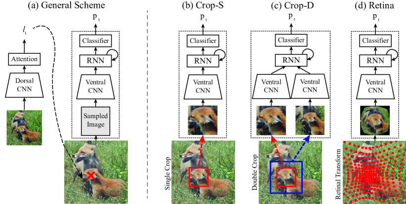
Figure 1: Recurrent models for eye movement and visual recognition. (a) The model architecture includes two streams: the dorsal (left) and ventral (right) streams. The dorsal stream has a broad field of view and generates a fixation point ($l_{t}$) at a step (or glance). The ventral stream takes selective samples around the fixation, extract a representation, accumulates the representations across multiple glances for object recognition ($p_{t}$). Using this general scheme, we design and test three different implementations of the ventral stream, namely Crop-S, Crop-D, and Retina, illustrated in (b) through (d). (b) Crop-S crops a small image region (shown as the red box) around the fixation. (c) Crop-D crops two regions (shown as the red and blue boxes) around the fixation and samples them with different resolution such that the same number of samples is extracted from either region. (d) Retina applies retinal transformation and extracts non-uniform samples with respect to the fixation. Those models use the same architecture for the dorsal stream, for which the weights are learned separately alongside the different ventral stream models.

Spatial attention allows the brain to selectively focus visual processing on salient parts, while omitting insignificant parts or less informative background. As time permits, humans can attend to more locations in the visual field and move the eyes to sample distinct information. This recurrent process likely makes human vision more robust. When humans are given very limited time ($\sim$70ms or less) to observe an image, the brain has inadequate time to take more than one glance; under this condition, humans are also prone to make mistakes on the same adversarial examples that fool computer vision [11]. Such time-limited observation is believed to preclude recurrent attention, feedback processes, and eye movement and makes the brain’s visual processing feedforward-only, similar to CNNs [12, 13, 14]. As such, feedforward-only visual inference may be more susceptible to adversarial noises for both human and computer vision.

The human eyes may also help adversarial robustness [15]. The retina distorts and samples the visual input with different resolution, density, and acuity depending on the relative distance to the point of fixation (i.e., eccentricity). When an object falls within the fovea, it is sampled with higher acuity and resolution than it is in the periphery. During saccadic eye movements, the retinal samples of an object vary over time and represent the same object with varying resolution, scales, and features [16, 17, 18, 19, 20]. When eye movements are not prefixed but attention-driven, retinal transformation guided by and combined with recurrent attention give rise to an adaptive and dynamical system for image recognition, against which adversarial attacks have not been tested.

Here, we design a recurrent neural network inspired by human eyes and brains, and evaluate its adversarial robustness. The model includes three modules: an input sampler that takes retinal samples around the fixation, an attention network that mimics the brain’s dorsal visual pathway and guides where to look next, and a recognition network that mimics the ventral visual pathway and represents the retinal samples recurrently for object recognition. As illustrated in Fig. 1, we design three variations of such a model. Each of them uses a different strategy for sampling visual input with respect to the point of fixation, including cropping with a single field of view, with two fields of view, or applying retinal foveation and non-uniform sampling. These models all attempt to mimic the brain’s ability to engage saccadic eye movement and recurrent neural processing [14, 21]. We hypothesize that the model using eye-like, retinal transformation can progressively refine the perceptual decision and improve robustness against adversarial perturbations as it uses a longer time to take more glances at an image under attack.

2 Related Work

2.1 Adversarial Attacks

An adversarial attack refers to an attempt to deceive machine learning models by adding carefully designed perturbations to an input image [1, 2, 3, 4, 5]. The perturbation, known as adversarial noise, can be optimized with the projected gradient descent (PGD) [4], fast gradient sign method [1] and Carlini & Wagner attack [3], among others. To counteract adversarial noise, defensive methods have been proposed [1, 22, 23, 24] but still remain vulnerable [5, 3, 25].

Humans do not seem to suffer from the same vulnerability, especially when enough time is available for humans to observe the image under attack [11]. This distinction has motivated prior works to take inspiration from human vision for computer vision. For example, Luo and colleagues have found that allowing models to fixate to different image regions can alleviate the effect of adversarial noise [26]. More recently, Dapello and colleagues [27] show that attaching a block with properties of V1 at the front of feed-forward CNNs, can make CNNs more robust. Huang et al. [28] demonstrate that a neural network with predictive coding improves adversarial robustness.

Vuyyuru and colleagues [15] demonstrate that non-uniform spatial sampling and varying receptive fields that mimic the retinal transformation in the primate retina can also improve the robustness against adversarial attacks. Harrington and colleagues [29] show that the representation robust against adversiarial noises is more attributable to processing information from the periphery, as opposed to the fovea.

In line with the related work, we also explore biologically inspired computational mechanisms for adversarial robustness. Similar to [15], we use a retina-like front-end to generate fixation-dependent retinal input for image recognition. A notable distinction is that Vuyyuru prefixes the points of fixation, whereas in our study, the fixation is adaptive and inferred via an attention module that learns learn where to look next. As such, our model adaptively and iteratively samples an image into time-varying retinal patterns, similar to retinal input to the brain during saccadic eye movement.

2.2 Recurrent Attention

A crucial difference between human and machine vision is that humans explore images or scenes by directing attention with eye movement (overt attention) or without eye movement (covert attention). Prior works have attempted to make machines solve downstream tasks by teaching them where to look through a recurrent process. Given an attention focus (or fixation point), the attended region can be cropped at various resolutions or scales [30, 31, 32, 33]. Arguably better than hard cropping, the attended region may be subject to retinal transformation [15, 8, 34] or polar transformation [35] inspired by the primate retina [6, 36, 37, 38]. For covert attention, models generate and apply soft weightings for all features and locations depending on their relative importance [31, 39, 40].

These recurrent attention models are similar to the human brains. Because of this similarity, understanding recurrent attention models would provide insights into the adversarial robustness of human vision. However, despite their importance, recurrent attention models have rarely been the focus of research compared to their counterpart, feedforward CNNs. In the current work, we design and test different recurrent attention models, and show how they are affected by adversarial noise as more recurrent steps are deployed.

3 Method

As illustrated in Fig. 1(a), the dorsal stream has a wide field of view that covers the whole image sampled with lower resolution. It learns spatial attention, predicts where to look next, and passes the predicted fixation ($l_{t}$) to the ventral stream. The ventral stream has a narrow field of view around the fixation, samples the input, learns to represent the samples for each fixation, recurrently accumulates the representation across different fixations, and outputs the probability in image classification ($p_{t}$).

Specifically, the dorsal stream includes two modules: DorsalCNN and Attention. The ventral stream includes VentralCNN, RNN and Classifier. Three model variations shown in Fig. 1 (b), (c), (d) all share the same architecture for the dorsal stream, but use different sampling strategies for the ventral stream: a single cropped field of view (Crop-S), double cropped field of views with different resolution but the same matrix size (Crop-D), and retinal sampling (Retina). See details below.

3.1 Image Sampling

Single Crop The model Crop-S crops a rectangular patch around the fixated location as the input to the ventral stream (Fig 1 (b)).

Double Crop The model Crop-D processes two rectangular patches around the same fixation point, as shown in Fig 1 (c), with different scales and resolution. They are further resized to have the same matrix size.

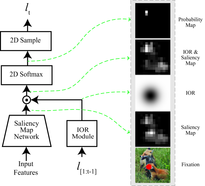
Figure 2: Details of the Attention module in the dorsal stream. Attention produces 2D saliency map and fixation point at time step $t$ ($l_{t}$). Intermediate representations from each module are shown on the right.

Retinal Sampling We design retinal sampling by the knowledge about biological visual systems. In primate visual systems, both retinal ganglion cells and neurons at early visual areas have increasingly larger receptive fields yet lower resolution at higher eccentricity relative to where the eyes are fixated in visual field [9, 10, 41]. In addition, more cells and neurons are devoted to the central vision than to peripheral vision [6, 7, 8]. Inspired by these properties, we design an input layer with two steps: 1) foveated imaging and 2) non-uniform sampling.

Foveated imaging [42, 43] varies image resolution and acuity along eccentricity: higher resolution around the fixation and progressively lower resolution towards the periphery. We implement this by applying a larger Gaussian kernel to peripheral regions but a smaller kernel to the central region, resulting in greater smoothness in the periphery. More details are included in Appendix A. Since each foveated image is transformed from the original image with a varying extent of spatial blurring, the feed-forward convolutional layers effectively have eccentricity-dependent receptive fields. This effect is similar to how biases from different receptive fields in the retina are passed to downstream visual areas.

Retinal sampling collects non-uniform discrete samples from the foveated image. Fig. 1(d) shows an example of retinal sampling points and the resulting retinal image. Suppose that we want to sample an $N\times N$ foveated image to fill an $n\times n$ retinal image with $n<N$. We first calculate the eccentricity $e(x,y;f_{x},f_{y})$ of any pixel location $(x,y)$ with respect to the fixation point $(f_{x},f_{y})$ in the foveated image (Eq. 1). Similarly we calculate $\rho(i,j;f_{i},f_{j})$ as the distance from fixation $(f_{i},f_{j})$ to pixel $(i,j)$ (Eq. 2) in the retinal image.

$$e(x,y;f_{x},f_{y}) =\|(x,y)-(f_{x},f_{y})\|_{2}$$ (1)

$$\quad\rho(i,j;f_{i},f_{j}) =\|(i,j)-(f_{i},f_{j})\|_{2}$$ (2)

We then relate the eccentricity in the foveated image $e$ to $\rho$ of the retinal image through a non-linear mapping function $g(\rho)$ (Eq. 3).

$$e=g(\rho)=\frac{N\sinh(\rho\cdot b\frac{2}{N})}{2\sinh(b\frac{n}{N})}$$ (3)

Here, $b\in\mathbb{R}^{+}$ is a hyper-parameter. Its value controls the degree of non-uniform sampling. When there is no retinal sampling, or $b$ is very small, it can be considered that an image is under the fovea, therefore visual acuity is high at everywhere sampled. As $b$ becomes larger, the fovea area decreases and the periphery increases, while the retinal image is increasingly distorted relative to the original image (See Appendix B and Fig. 3(c) for examples).

3.2 Dorsal Stream

The dorsal stream includes DorsalCNN and Attention module. The input to the dorsal stream is an image with the full view, but in a low resolution. The DorsalCNN is a stack of convolutional layers. Attention determines the next location to focus on. It uses the feature maps from all layers from DorsalCNN, after they are resized to the same size and then concatenated along the channel dimension. Fig. 2 shows the architecture of the attention module. To predict the next fixation point ($l_{t}$), the module maps salient regions with a Saliency Map Network. It includes a convolutional layer with $3\times 3$ kernels and outputs a 2D saliency map [44, 45], highlighting the candidate regions for the next fixation.

To prevent future fixations returning to the previously attended regions, the inhibition-of-return (IOR) module (IOR-Module) [46, 47] reduces the saliency of previously attended regions. Specifically, the IOR at time $t$ is expressed as below.

$$\textbf{ IOR}(t)=\texttt{IOR-Module}(\bm{l}_{1:t})=\textbf{ReLU}\Big{(}\bm{1}-\sum_{\tau=1}^{t}G(\bm{\mu}=\bm{l}_{\tau},\bm{\Sigma}=\sigma^{2}\bm{I})\Big{)}$$ (4)

Here, $G$ is a normalized 2D Gaussian function centered at $\bm{l}_{\tau}$ with a standard deviation $\sigma$ at the $\tau$-th step. Its values are normalized so that the maximum equals 1. We sum the normalized Gaussian kernels across all previous time steps to prohibit the future fixations to go back to the previously visited locations. Subtracting the accumulated Gaussian kernels from a matrix of ones creates a soft mask with high values at unattended regions but low values at previously attended regions. Applying this mask to the saliency map by element-wise multiplication followed by softmax gives rise to a 2D probability map based on which the next fixation is randomly sampled. Fig. 2 shows typical examples of the saliency map, IOR, and the prediction of next fixation point.

The dorsal stream is trained with reinforcement learning based on the REINFORCE algorithm [48]. At time $t$, the fixation $\bm{l}_{t}$ generated by the attention module results in a new class prediction $p_{t}$ by the recognition pathway (ventral stream). The reward $r_{t}$ of choosing $\bm{l}_{t}$ as the fixation is calculated as the reduced classification loss relative to the previous time step $r_{t}=CE(p_{t-1},\text{label})-CE(p_{t},\text{label})$, where $CE$ is the cross-entropy loss. The goal of reinforcement learning is to maximize the discounted sum of rewards, $R=\sum_{t=1}^{T}\gamma^{t-1}r_{t}$, where $\gamma\in(0,1)$ is the discount factor and it is set as 0.8.

3.3 Ventral Stream

The recognition pathway includes VentralCNN, RNN and Classifier stacked as shown in Fig. 1. VentralCNN consists of a stack of convolutional layers to extract features from the retinal samples at each time step. The extracted features are passed forward to a recurrent neural network (RNN) with gated recurrent units [49]. The RNN learns to accumulate information across different fixation points, which are then used for object recognition at the Classifier (a fully-connected layer) at every time step $t$. The learning objective is to minimize the the cross entropy losses summed across $T$ time steps.

3.4 Implementation Details

Convolutional layers in VentralCNN and DorsalCNN have the same architecture (but distinct parameters), and they all have convolutional layers using $3\times 3$ kernels with stride equal to $1$. VentralCNN and DorsalCNN have $\texttt{Conv}(64)\times 2\to\texttt{MaxPool}\to\texttt{Conv}(128)\times 2\to\texttt{MaxPool}\to\texttt{Conv}(256)\times 2\to\texttt{MaxPool}\to\texttt{Conv}(512)\times 2$, where $\texttt{Conv}(C)\times k$ represents $k$ convolutional layers with $C$ channels. MaxPool has a kernel size of $2$ and a stride of $2$. The sampled images for VentralCNN and DorsalCNN are in the size of $64\times 64$ and $128\times 128$ respectively. The dorsal and the ventral stream as shown in Fig. 1 are trained together. For the Crop-D model, the same VentralCNN sharing the weights is used to extract features from the both patches, and the resulting features are summed to be forwarded to the next module. Code and data are publicly available.

4 Experiments

We train these three models (Crop-S, Crop-D and Retina) for single-label classification, and evaluate their adversarial robustness. As additional baseline models, we also trained a model with feedforward CNN (FF-CNN) and a model with recurrent attention, but without overt eye movements (S3TA [39]). None of the models under comparison is trained with adversarial training, since our focus is on the model architecture, instead of learning strategies.

For training data, we randomly sample $100$ classes from ILSVRC2012 [50] with $1,000$ classes, and form ImageNet100. All dynamical models (Crop-S, Crop-D, Retina and S3TA) are trained while these models take four sequential gazes to an image (one gaze for each step). Table 1 includes the top-1 accuracy on ImageNet100’s validation set for all models, and summarizes their properties. Fig. 3(a) demonstrates the learned fixation points for each model. The first four fixations are placed on the foreground objects. For the retinal sampling, the hyper-parameter $b$ is set to $12.0$, if not specified otherwise.

Table 1: Summary of the models.

Model	Top-1 Accs	Input Type	Attention
Retina	75.56%	Retinal Image	Overt
Crop-D	81.21%	Double Crop	Overt
Crop-S	75.14%	Single Crop	Overt
S3TA	83.12%	Whole Image	Covert
FF-CNN	81.75%	Whole Image	-

Table 2: Attack success rates of the models.

Model		Untargeted					Targeted
	$\epsilon$:	2e-3	3e-3	5e-3	7e-3		3e-3	5e-3	7e-3	1e-2
Retina		28.7%	43.1%	65.5%	79.2%		4.3%	12.8%	30.7%	56.8%
Crop-D		51.0%	71.5%	90.9%	96.7%		20.0%	58.8%	84.6%	96.7%
Crop-S		64.4%	82.1%	94.1%	97.9%		31.9%	71.4%	88.2%	96.7%
S3TA		94.4%	98.1%	99.8%	99.9%		72.6%	93.0%	99.2%	100.0%
FF-CNN		90.1%	96.9%	99.3%	99.6%		83.5%	98.4%	99.5%	99.8%

4.1 Adversarial Attacks

We evaluate adversarial robustness of the models trained on ImageNet100. Projected gradient descent (PGD) with $L_{\infty}$ is used while varying the maximum perturbation budget allowed ($\epsilon$). We iterate PGD for 100 times with the step size at $\epsilon/20$. All the sampling methods (Retinal transformation and image crop) are fully differentiable.

The dynamical models (Crop-S, Crop-D, Retina and S3TA) are set to take twelve gazes at each image under the untargeted/targeted attack to minimize/maximize the prediction probability of true/target class from all gazes. To reflect the stochastic nature of eye movements [51, 52], Gaussian noise (with 0 mean and 0.1 standard deviation) is added to the fixation points generated from the models (Crop-S, Crop-D and Retina), and Expectation over Transformation (EOT) [5] is used to deal with the randomness. In our experiments, we average the gradients over 40 iterations. Considering the huge amount of computational costs from 100 iterations of PGD and 40 iterations from EOT, we further sample the validation set of ImageNet100 to include $1,000$ images to reduce computational costs.

4.2 Effects of retinal transformation

Table 2 shows the ASR of dynamical models at the $12$-th step given adversarial examples with various adversarial noise levels, epsilon ($\epsilon$). The result shows that the models with overt attention (Crop-S, Crop-D and Retina) are more robust than the covert attention (S3TA). Consistent with previous findings, we observe that combining multi-resolution patches (Crop-D) is more robust than a single-resolution patch (in Crop-S) [15]. The model Retina maintains the highest robustness compared to other baseline models, and outperforms Crop-S and Crop-D by a large margin. This result suggests that non-uniform retinal transformation is a key mechanism for adversarial robustness among the three sampling strategies.

4.3 Effects of the number of recurrent steps

Unlike feed-forward CNNs, dynamical models can vary and unroll their computational graphs with increasing time. Hence, we evaluate these models’ ASR as a function of time at each recurrent inference step. Fig. 4(a) visualizes ASR at the $12$-th step of the targeted attack from Table 2 including adversarially trained FF-CNN (FF-CNN-AT), which acheives highest robustness. Fig. 4(b) shows ASR for all $24$ steps from the targeted PGD attack. All models except for the model Retina appear to maintain or increase ASR by taking more glances for object recognition. In contrast, the model Retina increases its robustness during the steps both under ($1\sim 12$ steps) and after ($12\sim 24$ steps) the attack.

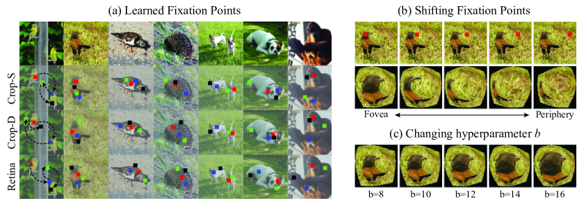
Figure 3: (a) Learned fixations from the first four steps. From the first fixation to the last fixations are marked as Red-Blue-Green-Black. First column presents exemplar attention shifts. (b) Visualization of the retinal transformation as the object is shifted from the fovea to the periphery. (c) Examples of the retinal transformation as the hyperparameter $b$ is changing from $8$ to $16$.

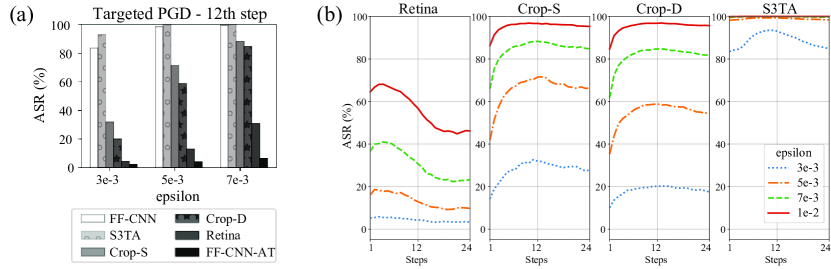
Figure 4: Results of targeted PGD attack. (a) Attack success rate (ASR) from $12$th step. (b) ASR from all steps.

4.4 Effect of attention-guided eye movement

To intuitively understand this difference, we visualize the regions that are affected by the adversarial attack for each model (Fig. 5). We first obtain two adversarial images from each of the three models (Crop-S, Crop-D and Retina), with one or two fixations. The first fixation is from the model’s learned attention, while the second fixation is always placed on the lower left corner of the images, making the first fixation point be located in the periphery of the second fixation. The first (blue) and the second (red) fixations are marked on image examples in the first row of Fig. 5(b). Two adversarial images from each model are generated under the targeted PGD attack: one deploying only the first fixation (blue), and the other deploying both two fixations. The resulting adversarial images are not shown in Fig. 5. The same Gaussian noise and the targeted attack used for Table 2 and Fig. 4 are used again for the experiment.

Once the adversarial images are generated, the models take them as input and perform a recognition task by making fixations on all the possible locations on the images (Fig. 5(a)). In this experiment, a $32\times 32$-sized regular grid (invisible) is placed on the adversarial image (shown in the bottom of Fig. 5(a)) as the possible locations for fixations. The output prediction probability of the target class (i.e., a randomly sampled class used for targeted attack) are recorded into the corresponding location in the new $32\times 32$ grid (Fig. 5(a), top). Object recognition is performed independently at each fixation, which means the RNN in the ventral stream is re-initialized at every test step. Therefore, we can view the models are performing one-step recognition for each location in the $32\times 32$ grid.

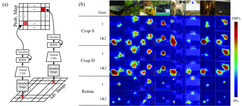
Figure 5: (a) Experiment methods for the adversarial probability map. Adversarial probability map is obtained by recording the output probability of target class from the models while the fixation is systematically changed to all the image regions. (b) First row: Examples of the original images and fixations (blue dot: first fixation, red dot: second fixation). From the second row: Examples of adversarial probability maps when 1) only the first fixation is allowed and 2) first two fixations are allowed for each model.

Fig. 5(b) shows the resulting probability maps for the target class from the models. Red regions suggests a vulnerable fixation spot when the model is under the adversarial attack. As can be seen in Fig. 5(b), the locations near the attacked fixation points are more vulnerable. However, although the fixations are the same across all models, the area that is highly affected by the adversarial attack is different for distinct models. The model Retina shows the smallest area affected by the adversarial attack compared to the Crop-S and Crop-D models. By comparing the probability maps from a single fixation and two fixations, we observed that the attacked area near the first fixation was persistently affected during the second attack. However, for the Retina model, the area affected from the attack at first fixation is reduced after including the second fixation.

This observations can be attributed to the fact that the convolutional operation on the retinal images does not maintain the property of translational equivariance, while the convolution on the images in regular grid does. When the fixation in Crop-S or Crop-D changes a little bit, the representations after convolutional operations will be simply shifted to the new fixation location. However, for the model Retina, small changes in the fixation will result in large changes in the retinal images after foveation and non-uniform sampling. This may further alter its representation significantly in the stacked CNN layers. This fixation-dependent representation is not a simple translation but a change of the whole layout. Therefore, the adversarial noise generated at the certain fixation does not necessarily fool the Retina model when a fixation point is made on other locations. Even the adversarial effect across gazes mitigates each other.

This is in line with the human brain, where foveal vision and peripheral vision have different functional roles. The foveal vision focuses on object recognition, while the peripheral vision has better adversarial robustness [53, 54, 29]. In Fig. 5, when the first fixation is made on the object, the adversarial noise is calculated based on the object in the foveal vision. Then when the second fixation is set at the corner, the object is placed in the peripheral vision. Because of this difference, the adversarial noise from the foveal vision (from the first fixation) fools the model less effectively when it is placed on the peripheral vision (from the second fixation).

5 Discussions

Our findings suggest that incorporating brain-inspired mechanisms makes computer vision more robust against adversarial noise. Specifically, retinal sampling, adaptive eye movement, and recurrent processing collectively improve adversarial robustness.

Models that incorporate retinal transformation appear the most robust among all models tested in this study. Retinal sampling likely brings two benefits to adversarial robustness. Adversarial perturbations generated for a retinal pattern with any given fixation is difficult to be generalized to the retinal patterns with other fixations; in contrast, for models applied to a regular grid input, the perturbations applied to one location are generalizable to other locations. Secondly, as the eyes move and fixate to different locations, the resulting retinal patterns represent the same objects with different features, resolution and scales. This is expected to increasingly augment the input data with a wide range of views, scales, and orientation. Models with retinal sampling are also expected to be computationally efficient, especially when the visual field is large or the visual content is sparse.

Models with adaptive eye movement are harder to attack. In the absence of time limitation, a model may look at an image for many times and attend to a different region at each time. If the attacker does not have access to where the model looks next, results from our experiments suggest that taking more glances beyond what the attacker has access to likely brings a mechanism for the model to correct the mistake on adversarial images, especially if eye movement is stochastic and adaptive. Additionally, our experiments show that the models with overt eye movement (i.e., overt attention) are generally more robust than those with covert attention.

The brain-inspired mechanisms are much beyond what we have explored and should be studied and substantiated further to enable better and more robust computer vision [27, 15], as well as to help understand the mechanism and behavior of human vision.

Appendix A Foveated Image

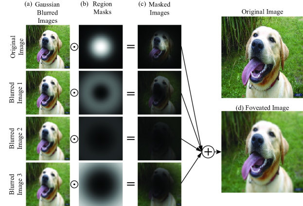
Figure 6: Illustration of the foveated image generated from an example image, when the fixation is at the image center. (a) The original image is blurred by applying different Gaussian kernels, (b) region masks applied to the blurred images. The black and white colors represent the range of values ($0$, $1$). (c) Results of element-wise multiplication of (a) and (b). (d) The foveated image by summing up the masked images.

In the foveated image, the foveated region maintains high acuity, but the periphery has reduced acuity. To implement the eccentricity-dependent acuity, we apply different levels of Gaussian blur based on the eccentricity. Here, we assume that the fixation is at the center of an image. Similar procedures can be generalized to non-centered fixation.

To illustrate a varying blurring effect, we use three 2D isotropic Gaussian kernels, $\bm{K}_{b1}$, $\bm{K}_{b2}$ and $\bm{K}_{b3}$. The kernel $\bm{K}_{bi}$ ($i\in[1,2,3]$) is in size $7\times 7$ and have a variance $\sigma_{bi}^{2}$. The $\sigma_{b1}$, $\sigma_{b2}$ and $\sigma_{b3}$ are set to 1, 3 and 5, respectively in this study.

Firstly, the Gaussian kernels $\bm{K}_{b1}$, $\bm{K}_{b2}$ and $\bm{K}_{b3}$ are separately applied to the original image, resulting in blurred images, $\bm{A}_{b1}$, $\bm{A}_{b2}$ and $\bm{A}_{b3}$. The original image ($\bm{A}$) and the blurred images are shown in Fig. 6(a).

Secondly, region masks are produced. The region masks are used to confine the regions with a specific level of blurring. The masks appear as concentric rings. They act as filters to pass the image with the desired resolution to the target area. Applying such masks to the blurred images makes the blurring dependent on the eccentricity. For a foveated image, a region mask designed to pass the fovea region is applied to an image with original resolution (Fig. 6(b) top row). For the periphery, region masks for the peripheral regions are applied to the blurred images (shown in Fig. 6(b) $2$nd, $3$rd and $4$th row from the top).

To generate region masks, 2D isotropic Gaussian kernels are first generated. The Gaussian kernels are denoted as $\bm{T}_{t1}$, $\bm{T}_{t2}$ and $\bm{T}_{t3}$, and they are in size $224\times 224$. $\bm{T}_{t1}$, $\bm{T}_{t2}$ and $\bm{T}_{t3}$ have means at the fixated location and variances $\sigma_{t1}^{2}$, $\sigma_{t2}^{2}$ and $\sigma_{t3}^{2}$, respectively (In this study, $\sigma_{t1}=40$, $\sigma_{t2}=70$, $\sigma_{t3}=90$). The generated Gaussian kernels are normalized to make their maximal amplitude $1.0$. The region masks $\bm{M}_{1}$, $\bm{M}_{2}$, $\bm{M}_{3}$ and $\bm{M}_{4}$ are generated as Eq. 5a-5d

$$\bm{M}_{1} =\bm{T}_{t1}$$ (5a)

$$\bm{M}_{2} =\bm{T}_{t2}-\bm{T}_{t1}$$ (5b)

$$\bm{M}_{3} =\bm{T}_{t3}-\bm{T}_{t2}$$ (5c)

$$\bm{M}_{4} =\bm{1}-\bm{T}_{t3}$$ (5d)

where $\bm{1}$ is a 2D matrix filled with ones whose size is identical to $\bm{T}_{t3}$ The region masks are shown in Fig. 6(b) and it can be checked that each region mask passes distinct image regions based on the eccentricity.

Once the blurred images and the region masks are obtained, the region masks are applied to the corresponding original and blurred images as element-wise multiplications (Eq. 6a-6d).

$$\bm{A}_{m1} =\bm{A}\odot\bm{T}_{t1}$$ (6a)

$$\bm{A}_{m2} =\bm{A}_{b1}\odot\bm{T}_{t2}$$ (6b)

$$\bm{A}_{m3} =\bm{A}_{b2}\odot\bm{T}_{t3}$$ (6c)

$$\bm{A}_{m4} =\bm{A}_{b3}\odot\bm{T}_{t4}$$ (6d)

where the operation $\odot$ is an element-wise multiplication. The first region mask $\bm{T}_{t1}$ designed to pass the center of fixation is applied to the original image so that the foveated image maintains high acuity in the fixated region. On the contrary, the region masks assigned to the peripheral regions are applied to the corresponding blurred images. The masked images are shown in Fig. 6(c).

Lastly, the masked images are summed together to produce the foveated image.

$$\text{Foveated Image}=\bm{A}_{m1}+\bm{A}_{m2}+\bm{A}_{m3}+\bm{A}_{m4}$$ (7)

The resulting image is shown in Fig. 6(d). In the foveated image, the region near the fixation maintains the high acuity, and the periphery regions are gradually blurred as the eccentricity grows.

Appendix B Effect of $b$ on the fovea size

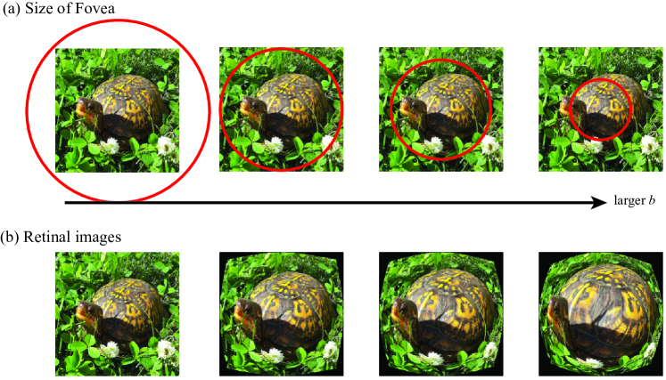
Figure 7: Illustration of an effect of the control variable $b$ on the retinal image. (a) Original image and size of the fovea. Red circle represents (virtual) boarder between the fovea and the periphery. (b) Retinal image corresponding to the size of the fovea.

When $b$ is small, the fovea is large enough to include an image. Therefore, all the image region is in high resolution (leftmost images in Fig 7 (a) and (b)). As $b$ becomes larger, the fovea becomes smaller, and more image area is included in the periphery.

The models of Crop-S, Crop-D and Retina are trained in two stages. In the first stage, the fixations are randomly generated, and only the ventral stream is trained for object classification. In the second stage, the fixations are generated using the dorsal stream and both the dorsal and the ventral streams are trained all together.

Appendix C Retinal Transformation: Examples

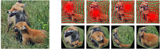
Figure 8: Examples of the retinal transformation. Left: Original image, Right: Retinal sampling grid and resulting retinal images.

Appendix D Adversarial Attack

We use AdverTorch toolbox for adversarial attack algorithms [55].

D.1 PGD Attack

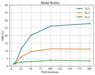
Figure 9: Attack convergence with the number of iterations of PGD.

Fig. 9 shows the performance of PGD attack with the same settings in Table 2 (targeted attack) using different numbers of iterations. The effect of PGD attack increases as the number of iterations grows and there are no significant changes after 100 iterations.

D.2 Adversarial Robustness Against SPSA and FGSM Attack

Table 3: Results of untargeted FGSM attacks (ASR)

eps	PGD	FGSM
2e-3	28.7%	21.99%
3e-3	43.1%	31.29%
5e-3	65.5%	44.01%
7e-3	79.2%	53.56%

Table 4: Results of untargeted SPSA attacks (ASR)

eps	PGD	SPSA
7e-3	78.3%	5.4%
1e-2	90.7%	13.5%
2e-2	100.0%	20.8%
3e-2	100.0%	27.0%

We further test adversarial robustness on SPSA [56] attack and fast gradient sign method (FGSM) [1] attack. Table 3 presents top-1 accuracy under untargeted FGSM attack. The results demonstrate that the iterative method (PGD) outperforms the single-step method (FGSM).

For SPSA attack (Table 4), batch size $4,096$ and $100$ iteration are used with epsilons $7e-3,1e-2,2e-2,3e-2$. For SPSA attack, we further sample the validation set used for experiments in the main paper to include only $100$ images to maintain computational costs of SPSA in a reasonable range. Table 4 shows ASR of the Retina model on the $100$ images for both PGD and SPSA. PGD (white box attack) is a stronger attack than SPSA (black box attack).

Appendix E Limitation

One of the limitations of the current work is that the model Retina under-performs other models (FF-CNN and Crop-D) in object recognition tasks on clean images (Table 1). Although the object recognition task is not the scope of this paper, both the recognition performance and the adversarial robustness can be of concern for some applications.

We conjecture that the less effective recognition performance of the model Retina can be attributed to the fact that the dataset (ImageNet [50]) is different from the visual scenes that we humans encounter every day. Lots of images in ImageNet include only one object in each image, and the objects usually take a large portion of the image area. For human visions, object recognition mostly relies on the information from the foveal vision, except for some cases when the objects are large (such as buildings) [57, 58, 59]. However, because objects in ImageNet are usually large, the foveal vision from the Retina model cannot cover the objects. Therefore, peripheral vision, which produces less reliable features for object recognition, heavily takes part in the recognition process. Because of this, the Retina model is less effective in object recognition on ImageNet data. If the models are trained in a more realistic dataset (including multiple and smaller objects, so that the foveal vision is enough to cover the objects), the performance gap between the Retina and Crop-D might be reduced.

Appendix F Negative Impacts

In the current work, we designed models and compared their adversarial robustness. The models that we designed include key features of human visual systems (retinal transformation, eye movements, and recurrent processing), which are not the main focus of machine learning research. These biologically-plausible models are helpful to improve our understanding of the robustness of human visual systems by simulating features that only human visions have. At the same time, our study may provide means to attack human visual systems. Our study demonstrated that adversarial robustness of retinal transformation comes from the difference between central and peripheral visions. If an attack algorithm can deal with this center/periphery difference, it would be possible to attack human visual systems.

Appendix G ImageNet100

The randomly selected $100$ classes from $1000$ classes of ILSVRC2012 [50] are:

[n01496331 n01756291 n01833805 n02025239 n02100583 n02137549 n02480495 n02808440 n03124043 n03291819 n03770679 n03902125 n04201297 n04371430 n09246464 n01531178 n01768244 n01843383 n02028035 n02102480 n02138441 n02492660 n02834397 n03127747 n03388183 n03781244 n03956157 n04251144 n04399382 n09472597 n01630670 n01797886 n01847000 n02077923 n02105412 n02172182 n02504458 n02892201 n03131574 n03443371 n03785016 n04037443 n04275548 n04505470 n01644900 n01806143 n01871265 n02087046 n02106166 n02190166 n02640242 n02963159 n03180011 n03494278 n03796401 n04040759 n04325704 n04536866 n01667778 n01807496 n01872401 n02088632 n02108089 n02233338 n02701002 n02971356 n03216828 n03662601 n03837869 n04049303 n04335435 n04589890 n01669191 n01817953 n01968897 n02089078 n02113712 n02317335 n02787622 n02977058 n03249569 n03710193 n03877472 n04146614 n04355338 n04591713 n01694178 n01824575 n01980166 n02094258 n02119789 n02410509 n02795169 n03100240 n03272010 n03733131 n03877845 n04162706 n04356056 n07614500]

References

- [1] Ian J Goodfellow, Jonathon Shlens, and Christian Szegedy. Explaining and harnessing adversarial examples. arXiv preprint arXiv:1412.6572, 2014.
- [2] Christian Szegedy, Wojciech Zaremba, Ilya Sutskever, Joan Bruna, Dumitru Erhan, Ian Goodfellow, and Rob Fergus. Intriguing properties of neural networks. arXiv preprint arXiv:1312.6199, 2013.
- [3] Nicholas Carlini and David Wagner. Towards evaluating the robustness of neural networks. In 2017 ieee symposium on security and privacy (sp), pages 39--57. IEEE, 2017.
- [4] Aleksander Madry, Aleksandar Makelov, Ludwig Schmidt, Dimitris Tsipras, and Adrian Vladu. Towards deep learning models resistant to adversarial attacks. arXiv preprint arXiv:1706.06083, 2017.
- [5] Anish Athalye, Logan Engstrom, Andrew Ilyas, and Kevin Kwok. Synthesizing robust adversarial examples. In International conference on machine learning, pages 284--293. PMLR, 2018.
- [6] Christine A Curcio, Kenneth R Sloan, Robert E Kalina, and Anita E Hendrickson. Human photoreceptor topography. Journal of comparative neurology, 292(4):497--523, 1990.
- [7] Andrew B Watson. A formula for human retinal ganglion cell receptive field density as a function of visual field location. Journal of vision, 14(7):15--15, 2014.
- [8] Pouya Bashivan, Kohitij Kar, and James J DiCarlo. Neural population control via deep image synthesis. Science, 364(6439), 2019.
- [9] Ricardo Gattass, CG Gross, and JH Sandell. Visual topography of v2 in the macaque. Journal of Comparative Neurology, 201(4):519--539, 1981.
- [10] Ricardo Gattass, AP Sousa, and CG Gross. Visuotopic organization and extent of v3 and v4 of the macaque. Journal of neuroscience, 8(6):1831--1845, 1988.
- [11] Gamaleldin F Elsayed, Shreya Shankar, Brian Cheung, Nicolas Papernot, Alex Kurakin, Ian Goodfellow, and Jascha Sohl-Dickstein. Adversarial examples that fool both computer vision and time-limited humans. arXiv preprint arXiv:1802.08195, 2018.
- [12] Daniel J Felleman and David C Van Essen. Distributed hierarchical processing in the primate cerebral cortex. Cerebral cortex (New York, NY: 1991), 1(1):1--47, 1991.
- [13] Yasuko Sugase, Shigeru Yamane, Shoogo Ueno, and Kenji Kawano. Global and fine information coded by single neurons in the temporal visual cortex. Nature, 400(6747):869--873, 1999.
- [14] Victor AF Lamme and Pieter R Roelfsema. The distinct modes of vision offered by feedforward and recurrent processing. Trends in neurosciences, 23(11):571--579, 2000.
- [15] Manish Reddy Vuyyuru, Andrzej Banburski, Nishka Pant, and Tomaso Poggio. Biologically inspired mechanisms for adversarial robustness. Advances in Neural Information Processing Systems, 33:2135--2146, 2020.
- [16] Herman Bouma. Interaction effects in parafoveal letter recognition. Nature, 226(5241):177--178, 1970.
- [17] Jerome Y Lettvin et al. On seeing sidelong. The Sciences, 16(4):10--20, 1976.
- [18] Ruth Rosenholtz. Capabilities and limitations of peripheral vision. Annual review of vision science, 2:437--457, 2016.
- [19] Benjamin Balas, Lisa Nakano, and Ruth Rosenholtz. A summary-statistic representation in peripheral vision explains visual crowding. Journal of vision, 9(12):13--13, 2009.
- [20] Emma EM Stewart, Matteo Valsecchi, and Alexander C Schütz. A review of interactions between peripheral and foveal vision. Journal of vision, 20(12):2--2, 2020.
- [21] Kohitij Kar, Jonas Kubilius, Kailyn Schmidt, Elias B Issa, and James J DiCarlo. Evidence that recurrent circuits are critical to the ventral stream’s execution of core object recognition behavior. Nature neuroscience, 22(6):974--983, 2019.
- [22] Shixiang Gu and Luca Rigazio. Towards deep neural network architectures robust to adversarial examples. arXiv preprint arXiv:1412.5068, 2014.
- [23] Nicolas Papernot, Patrick McDaniel, Xi Wu, Somesh Jha, and Ananthram Swami. Distillation as a defense to adversarial perturbations against deep neural networks. In 2016 IEEE symposium on security and privacy (SP), pages 582--597. IEEE, 2016.
- [24] Cihang Xie, Jianyu Wang, Zhishuai Zhang, Zhou Ren, and Alan Yuille. Mitigating adversarial effects through randomization. arXiv preprint arXiv:1711.01991, 2017.
- [25] Warren He, James Wei, Xinyun Chen, Nicholas Carlini, and Dawn Song. Adversarial example defense: Ensembles of weak defenses are not strong. In 11th USENIX workshop on offensive technologies (WOOT 17), 2017.
- [26] Yan Luo, Xavier Boix, Gemma Roig, Tomaso Poggio, and Qi Zhao. Foveation-based mechanisms alleviate adversarial examples. arXiv preprint arXiv:1511.06292, 2015.
- [27] Joel Dapello, Tiago Marques, Martin Schrimpf, Franziska Geiger, David D Cox, and James J DiCarlo. Simulating a primary visual cortex at the front of cnns improves robustness to image perturbations. BioRxiv, 2020.
- [28] Yujia Huang, James Gornet, Sihui Dai, Zhiding Yu, Tan Nguyen, Doris Tsao, and Anima Anandkumar. Neural networks with recurrent generative feedback. Advances in Neural Information Processing Systems, 33:535--545, 2020.
- [29] Anne Harrington and Arturo Deza. Finding biological plausibility for adversarially robust features via metameric tasks. In SVRHM 2021 Workshop@ NeurIPS, 2021.
- [30] Yulin Wang, Kangchen Lv, Rui Huang, Shiji Song, Le Yang, and Gao Huang. Glance and focus: a dynamic approach to reducing spatial redundancy in image classification. arXiv preprint arXiv:2010.05300, 2020.
- [31] Kelvin Xu, Jimmy Ba, Ryan Kiros, Kyunghyun Cho, Aaron Courville, Ruslan Salakhudinov, Rich Zemel, and Yoshua Bengio. Show, attend and tell: Neural image caption generation with visual attention. In International conference on machine learning, pages 2048--2057. PMLR, 2015.
- [32] Volodymyr Mnih, Nicolas Heess, Alex Graves, and Koray Kavukcuoglu. Recurrent models of visual attention. arXiv preprint arXiv:1406.6247, 2014.
- [33] Pierre Sermanet, Andrea Frome, and Esteban Real. Attention for fine-grained categorization. arXiv preprint arXiv:1412.7054, 2014.
- [34] Emre Akbas and Miguel P Eckstein. Object detection through search with a foveated visual system. PLoS computational biology, 13(10):e1005743, 2017.
- [35] Carlos Esteves, Christine Allen-Blanchette, Xiaowei Zhou, and Kostas Daniilidis. Polar transformer networks. arXiv preprint arXiv:1709.01889, 2017.
- [36] LN Thibos, FE Cheney, and DJ Walsh. Retinal limits to the detection and resolution of gratings. JOSA A, 4(8):1524--1529, 1987.
- [37] Wilson S Geisler and David B Hamilton. Sampling-theory analysis of spatial vision. JOSA A, 3(1):62--70, 1986.
- [38] Nancy J Coletta and David R Williams. Psychophysical estimate of extrafoveal cone spacing. JOSA A, 4(8):1503--1513, 1987.
- [39] Daniel Zoran, Mike Chrzanowski, Po-Sen Huang, Sven Gowal, Alex Mott, and Pushmeet Kohli. Towards robust image classification using sequential attention models. In Proceedings of the IEEE/CVF conference on computer vision and pattern recognition, pages 9483--9492, 2020.
- [40] Andrew Jaegle, Felix Gimeno, Andy Brock, Oriol Vinyals, Andrew Zisserman, and Joao Carreira. Perceiver: General perception with iterative attention. In International Conference on Machine Learning, pages 4651--4664. PMLR, 2021.
- [41] Jeremy Freeman and Eero P Simoncelli. Metamers of the ventral stream. Nature neuroscience, 14(9):1195--1201, 2011.
- [42] Andrew T Duchowski, Nathan Cournia, and Hunter Murphy. Gaze-contingent displays: A review. CyberPsychology & Behavior, 7(6):621--634, 2004.
- [43] Jeffrey S Perry and Wilson S Geisler. Gaze-contingent real-time simulation of arbitrary visual fields. In Human vision and electronic imaging VII, volume 4662, pages 57--69. International Society for Optics and Photonics, 2002.
- [44] Laurent Itti, Christof Koch, and Ernst Niebur. A model of saliency-based visual attention for rapid scene analysis. IEEE Transactions on pattern analysis and machine intelligence, 20(11):1254--1259, 1998.
- [45] Christof Koch and Shimon Ullman. Shifts in selective visual attention: towards the underlying neural circuitry. In Matters of intelligence, pages 115--141. Springer, 1987.
- [46] Laurent Itti and Christof Koch. Computational modelling of visual attention. Nature reviews neuroscience, 2(3):194--203, 2001.
- [47] Michael I Posner and Yoav Cohen. Components of visual orienting. Attention and performance X: Control of language processes, 32:531--556, 1984.
- [48] Ronald J Williams. Simple statistical gradient-following algorithms for connectionist reinforcement learning. Machine learning, 8(3-4):229--256, 1992.
- [49] Junyoung Chung, Caglar Gulcehre, KyungHyun Cho, and Yoshua Bengio. Empirical evaluation of gated recurrent neural networks on sequence modeling. arXiv preprint arXiv:1412.3555, 2014.
- [50] Jia Deng, Wei Dong, Richard Socher, Li-Jia Li, Kai Li, and Li Fei-Fei. Imagenet: A large-scale hierarchical image database. In 2009 IEEE conference on computer vision and pattern recognition, pages 248--255. Ieee, 2009.
- [51] Yoram Burak, Uri Rokni, Markus Meister, and Haim Sompolinsky. Bayesian model of dynamic image stabilization in the visual system. Proceedings of the National Academy of Sciences, 107(45):19525--19530, 2010.
- [52] Xutao Kuang, Martina Poletti, Jonathan D Victor, and Michele Rucci. Temporal encoding of spatial information during active visual fixation. Current Biology, 22(6):510--514, 2012.
- [53] Nikos K Logothetis, Jon Pauls, and Tomaso Poggio. Shape representation in the inferior temporal cortex of monkeys. Current biology, 5(5):552--563, 1995.
- [54] Maximilian Riesenhuber and Tomaso Poggio. Hierarchical models of object recognition in cortex. Nature neuroscience, 2(11):1019--1025, 1999.
- [55] Gavin Weiguang Ding, Luyu Wang, and Xiaomeng Jin. AdverTorch v0.1: An adversarial robustness toolbox based on pytorch. arXiv preprint arXiv:1902.07623, 2019.
- [56] Jonathan Uesato, Brendan O’donoghue, Pushmeet Kohli, and Aaron Oord. Adversarial risk and the dangers of evaluating against weak attacks. In International Conference on Machine Learning, pages 5025--5034. PMLR, 2018.
- [57] Ifat Levy, Uri Hasson, Galia Avidan, Talma Hendler, and Rafael Malach. Center--periphery organization of human object areas. Nature neuroscience, 4(5):533--539, 2001.
- [58] Uri Hasson, Ifat Levy, Marlene Behrmann, Talma Hendler, and Rafael Malach. Eccentricity bias as an organizing principle for human high-order object areas. Neuron, 34(3):479--490, 2002.
- [59] Rafael Malach, Ifat Levy, and Uri Hasson. The topography of high-order human object areas. Trends in cognitive sciences, 6(4):176--184, 2002.