Computational Analysis of Impedance Transformations for Four-Wire Power Networks with Sparse Neutral Grounding

Frederik Geth frederik.geth@gmail.com 0000-0002-9345-2959 CSIRO EnergyNewcastleNSWAustralia Rahmat Heidari rahmat.heidarihaei@csiro.au 0000-0003-4835-2614 CSIRO EnergyNewcastleAustralia  and  Arpan Koirala arpan.koirala@kuleuven.be 0000-0003-4826-7137 KU Leuven / EnergyVilleLeuven / GenkBelgium
(2022)
Abstract.

In low-voltage distribution networks, the integration of novel energy technologies can be accelerated through advanced optimization-based analytics such as network state estimation and network-constrained dispatch engines for distributed energy resources. The scalability of distribution network optimization models is challenging due to phase unbalance and neutral voltage rise effects necessitating the use of 4 times as many voltage variables per bus than in transmission systems. This paper proposes a novel technique to limit this to a factor 3, exploiting common physical features of low-voltage networks specifically, where neutral grounding is sparse, as it is in many parts of the world. We validate the proposed approach in OpenDSS, by translating a number of published test cases to the reduced form, and observe that the proposed “phase-to-neutral” transformation is highly accurate for the common single-grounded low-voltage network configuration, and provides a high-quality approximation for other configurations. We finally provide numerical results for unbalanced power flow optimization problems using PowerModelsDistribution.jl, to illustrate the computational speed benefits of a factor of about 1.42.

unbalanced optimal power flow, continuous optimization, impedance transformation
journalyear: 2022copyright: acmcopyrightconference: The Thirteenth ACM International Conference on Future Energy Systems; June 28-July 1, 2022; Virtual Event, USAbooktitle: The Thirteenth ACM International Conference on Future Energy Systems (e-Energy ’22), June 28-July 1, 2022, Virtual Event, USAprice: 15.00conference: ACM e-Energy 2022; June 28 - July 1, 2022; virtual eventccs: Theory of computation Continuous optimizationccs: Theory of computation Network flowsccs: Software and its engineering Domain specific languagesccs: Computing methodologies Model verification and validationccs: Applied computing Multi-criterion optimization and decision-making

1. Introduction

1.1. Background on Public Four-wire Networks

Low-voltage (LV) networks are dealing with the integration of new technologies, including solar PV, home batteries and electric vehicles. Solving physics-based mathematical optimization problems in such networks is an interesting technology development opportunity (Claeys et al., 2021), with problems such as unbalanced network state estimation, distribution locational marginal pricing, network-constrained battery dispatch and EV charging coordination receiving significant attention by researchers.

Around the globe, many LV networks have a dual-voltage three-phase + neutral configuration (e.g. 400/230 V or 208/120 V), with grounding of the neutral only at the MV/LV transformer. This leads to situations where there can be a nontrivial amount of neutral voltage, a.k.a. neutral voltage shift, downstream of the transformer. Neutral voltage shift tends to negatively impact the voltage quality of the network, as it exacerbates phase-to-neutral voltage magnitude issues. Accurately capturing neutral voltage shift is therefore important, as it may limit the uptake of distributed energy resources.

Where the neutral is grounded, neutral current flows via the earth through a grounding rod111Sometimes first through an impedance.. The regularity of grounding depends on the network design principles, with“multi-grounded” and “single-grounded” being the two main approaches. In three-phase dual-voltage residential networks, grounding is probably near-universal on the wye-side of transformers, where the neutral point would otherwise be floating, which itself would not enable stable phase-to-neutral voltages. Nevertheless, neutral grounding can be performed additionally throughout the network when network codes allow for it – or demand it.

Furthermore, in the real world, cables and overhead lines induce current into the ground due to capacitive coupling with earth (nF/km) (Kersting, 2001)(Olivier et al., 2018). However, at 50 or 60 Hz the shunt admittance in LV networks is typically very small, and the voltage is low as well, so the shunt current contribution is limited in normal operation. Note that it is not expected that electrical devices owned by end-users inject a significant amount of current directly into the ground - that is typically considered a fault situation and is protected against by residual current devices a.k.a. ground fault circuit interrupters. Nevertheless, at medium voltage or higher, the line shunt currents may become significant in the overall current balance of the network at low load.

Industrial engineering software such as Digsilent PowerFactory and open-source power system research platforms such as OpenDSS (Dugan and McDermott, 2011) include scalable algorithms for steady-state simulation of voltage unbalance, neutral voltage rise in single and multi-grounded systems with capacitive coupling to ground (Ciric et al., 2003).

1.2. Research Question and Contributions

In the context of unbalanced power flow optimization problems, scalability remains crucial but challenging and commercial solutions are lacking (Claeys et al., 2022). Capturing neutral voltage rise usually means representing four complex-valued voltage variables per bus, one for each terminal $t\in\{a,b,c,n\}$. When one assumes the neutral is pervasively grounded (e.g. justifiable in a multi-grounded philosophy), Kron’s reduction of the neutral (Dorfler and Bullo, 2013) introduces minimal error, and enables elimination of the neutral voltage variables, which implies that the optimization problem may be solved faster (due to 25% fewer variables). However, this transformation can not capture neutral voltage rise accurately, and therefore it is not an attractive option for networks with a sparsely grounded neutral (e.g. single-grounded neutral) with significant load unbalance.

The central research question addressed in this paper is: ‘Is there an alternative to Kron’s reduction of the neutral that can capture neutral voltage rise, but equally enables a reduction in problem size from 4 to 3 complex voltage variables per bus?’ We therefore:

  • derive a novel “phase-to-neutral” transformation from first principles;

  • postulate conditions under which it is accurate;

  • analyze some of its properties;

  • run numerical experiments, using OpenDSS (Dugan and McDermott, 2011), to validate the approximation quality across a selection of LV and MV networks;

  • demonstrate the scalability advantages in a power flow optimization context, using PowerModelsDistribution (Fobes et al., 2020).

2. Phase-to-neutral Transformation

We first introduce our notation and derive a self-contained mathematical description of four-wire power flow with neutral grounding. The remainder of the section develops a linear transformation $\mathcal{T}:{\color[rgb]{.25,.25,.25}\mathbb{C}}^{4\times 4}\rightarrow{\color[rgb]{.25,.25,.25}\mathbb{C}}^{3\times 3}$, which is a generalization of ideas presented first in Koirala et al. (Koirala et al., 2019) when applied to series impedance matrices.

2.1. Symbols

Table 1 summarizes the vector and matrix symbols used in this article. A blue color indicates a complex variable, a brown color indicates a complex parameter, a red color indicates a real parameter. A bold typeface indicates a vector or matrix variables, a normal typeface is a scalar variable.

Table 1. Vector and matrix symbols
${\color[rgb]{0,0,1}\mathbf{U}_{{i}}}$ (V) Phase-to-ground voltage vector at bus $i$
${\color[rgb]{0,0,1}\mathbf{U}_{{i}}^{\text{pn}}}$ (V) Phase-to-neutral voltage vector at bus $i$
${\color[rgb]{0,0,1}\mathbf{I}_{{l}{i}{j}}}$ (A) Total current vector in line $l$ in the direction $i\rightarrow j$
${\color[rgb]{0,0,1}\mathbf{I}_{{l}{i}{j}}^{\text{{s}}}}$ (A) Series current vector in line $l$ in the direction $i\rightarrow j$
${\color[rgb]{0,0,1}\mathbf{I}_{{l}{i}{j}}^{\text{{sh}}}}$ (A) Shunt current vector in line $l$ in the direction $i\rightarrow j$
${\color[rgb]{0,0,1}\mathbf{I}_{d}}$ (A) Load $d$ current vector
${\color[rgb]{0,0,1}\mathbf{I}_{g}}$ (A) Generator $g$ current vector
${\color[rgb]{0,0,1}\mathbf{I}_{i}^{\text{g}}}$ (A) Bus $i$ grounding current vector
${\color[rgb]{.75,.5,.25}\mathbf{z}_{{l}}^{\text{{s}}}}$ (A) Series impedance matrix of line $l$
${\color[rgb]{1,0,0}\mathbf{T}}$ (-) Phase-to-neutral transformation matrix

2.2. Preliminaries

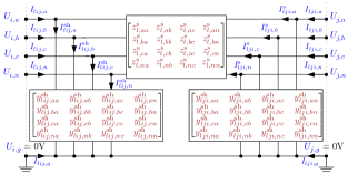
Fig. 1 defines the scalar symbols for the total, series and shunt current variables, phase-to-ground voltages, impedances for the (asymmetric) $\Pi$-section with phases ${\color[rgb]{1,0,0}\mathcal{P}}=\{a,b,c\}$ and neutral $n$, for a line $l$ between buses $i$ and $j$.

Refer to caption
Figure 1. Four-wire line model

The series impedance matrix of line $l$ is,

(1) $${\color[rgb]{.75,.5,.25}\mathbf{z}_{{l}}^{\text{{s}}}}=\begin{bmatrix}{\color[rgb]{.75,.5,.25}z_{{l},{a}{a}}^{\text{{s}}}}&{\color[rgb]{.75,.5,.25}z_{{l},{a}{b}}^{\text{{s}}}}&{\color[rgb]{.75,.5,.25}z_{{l},{a}{c}}^{\text{{s}}}}&{\color[rgb]{.75,.5,.25}z_{{l},{a}{n}}^{\text{{s}}}}\\ {\color[rgb]{.75,.5,.25}z_{{l},{b}{a}}^{\text{{s}}}}&{\color[rgb]{.75,.5,.25}z_{{l},{b}{b}}^{\text{{s}}}}&{\color[rgb]{.75,.5,.25}z_{{l},{b}{c}}^{\text{{s}}}}&{\color[rgb]{.75,.5,.25}z_{{l},{b}{n}}^{\text{{s}}}}\\ {\color[rgb]{.75,.5,.25}z_{{l},{c}{a}}^{\text{{s}}}}&{\color[rgb]{.75,.5,.25}z_{{l},{c}{b}}^{\text{{s}}}}&{\color[rgb]{.75,.5,.25}z_{{l},{c}{c}}^{\text{{s}}}}&{\color[rgb]{.75,.5,.25}z_{{l},{c}{n}}^{\text{{s}}}}\\ {\color[rgb]{.75,.5,.25}z_{{l},{n}{a}}^{\text{{s}}}}&{\color[rgb]{.75,.5,.25}z_{{l},{n}{b}}^{\text{{s}}}}&{\color[rgb]{.75,.5,.25}z_{{l},{n}{c}}^{\text{{s}}}}&{\color[rgb]{.75,.5,.25}z_{{l},{n}{n}}^{\text{{s}}}}\\ \end{bmatrix}.$$

In the real world, both the real and the imaginary part of the series impedance are symmetric and positive semidefinite, however we don’t need to assume this in the remainder of this work, and therefore define separate parameters for mutual induction, e.g. $a\rightarrow b$ and $b\rightarrow a$. The diagonal elements are called the self-impedances and the off-diagonal the mutual impedances. For convenient comparison of impedance transformations later, we define the do-nothing transformation $\mathcal{O}({\color[rgb]{.75,.5,.25}\mathbf{z}_{{l}}^{\text{{s}}}})={\color[rgb]{.75,.5,.25}\mathbf{z}_{{l}}^{\text{{s}}}}$.

We stack the scalar current variables (Fig. 1) in vectors to obtain the vector expression of conservation of current, linking the total current ${\color[rgb]{0,0,1}\mathbf{I}_{{l}{i}{j}}}$, series current ${\color[rgb]{0,0,1}\mathbf{I}_{{l}{i}{j}}^{\text{{s}}}}$ and shunt current ${\color[rgb]{0,0,1}\mathbf{I}_{{l}{i}{j}}^{\text{{sh}}}}$ in line $l$ in the direction $i\rightarrow j$,

(2) $${\color[rgb]{0,0,1}\mathbf{I}_{{l}{i}{j}}}=\begin{bmatrix}{\color[rgb]{0,0,1}I_{{l}{i}{j},{a}}}\\ {\color[rgb]{0,0,1}I_{{l}{i}{j},{b}}}\\ {\color[rgb]{0,0,1}I_{{l}{i}{j},{c}}}\\ {\color[rgb]{0,0,1}I_{{l}{i}{j},{n}}}\end{bmatrix}=\underbrace{\begin{bmatrix}{\color[rgb]{0,0,1}I_{{l}{i}{j},{a}}^{\text{{s}}}}\\ {\color[rgb]{0,0,1}I_{{l}{i}{j},{b}}^{\text{{s}}}}\\ {\color[rgb]{0,0,1}I_{{l}{i}{j},{c}}^{\text{{s}}}}\\ {\color[rgb]{0,0,1}I_{{l}{i}{j},{n}}^{\text{{s}}}}\end{bmatrix}}_{{\color[rgb]{0,0,1}\mathbf{I}_{{l}{i}{j}}^{\text{{s}}}}}+\underbrace{\begin{bmatrix}{\color[rgb]{0,0,1}I_{{l}{i}{j},{a}}^{\text{{sh}}}}\\ {\color[rgb]{0,0,1}I_{{l}{i}{j},{b}}^{\text{{sh}}}}\\ {\color[rgb]{0,0,1}I_{{l}{i}{j},{c}}^{\text{{sh}}}}\\ {\color[rgb]{0,0,1}I_{{l}{i}{j},{n}}^{\text{{sh}}}}\end{bmatrix}}_{{\color[rgb]{0,0,1}\mathbf{I}_{{l}{i}{j}}^{\text{{sh}}}}}={\color[rgb]{0,0,1}\mathbf{I}_{{l}{i}{j}}^{\text{{s}}}}+{\color[rgb]{0,0,1}\mathbf{I}_{{l}{i}{j}}^{\text{{sh}}}}.$$

The ground current for line $l$ in the direction $i\rightarrow j$ is,

(3) $${\color[rgb]{0,0,1}I_{{l}{i}{j},{g}}}=-({\color[rgb]{0,0,1}I_{{l}{i}{j},{a}}}+{\color[rgb]{0,0,1}I_{{l}{i}{j},{b}}}+{\color[rgb]{0,0,1}I_{{l}{i}{j},{c}}}+{\color[rgb]{0,0,1}I_{{l}{i}{j},{n}}})=-{\color[rgb]{1,0,0}\mathbf{1}}^{\text{T}}{\color[rgb]{0,0,1}\mathbf{I}_{{l}{i}{j}}}.$$

Next, we stack the depicted scalar voltage-to-ground222i.e. w.r.t. ${\color[rgb]{0,0,1}U_{{i},{g}}}=0$ V variables at bus $i$ (Fig. 1) in the vector ${\color[rgb]{0,0,1}\mathbf{U}_{{i}}}$ and derive the phase-to-neutral voltages ${\color[rgb]{0,0,1}\mathbf{U}_{{i}}^{\text{pn}}}$,

(4) $${\color[rgb]{0,0,1}\mathbf{U}_{{i}}}=\begin{bmatrix}{\color[rgb]{0,0,1}U_{{i},{a}}}\\ {\color[rgb]{0,0,1}U_{{i},{b}}}\\ {\color[rgb]{0,0,1}U_{{i},{c}}}\\ {\color[rgb]{0,0,1}U_{{i},{n}}}\end{bmatrix},{\color[rgb]{0,0,1}\mathbf{U}_{{i}}^{\text{pn}}}=\begin{bmatrix}{\color[rgb]{0,0,1}U_{{i},{a}{n}}}\\ {\color[rgb]{0,0,1}U_{{i},{b}{n}}}\\ {\color[rgb]{0,0,1}U_{{i},{c}{n}}}\end{bmatrix}=\underbrace{\begin{bmatrix}1&0&0&-1\\ 0&1&0&-1\\ 0&0&1&-1\\ \end{bmatrix}}_{{\color[rgb]{1,0,0}\mathbf{T}}}\begin{bmatrix}{\color[rgb]{0,0,1}U_{{i},{a}}}\\ {\color[rgb]{0,0,1}U_{{i},{b}}}\\ {\color[rgb]{0,0,1}U_{{i},{c}}}\\ {\color[rgb]{0,0,1}U_{{i},{n}}}\end{bmatrix}={\color[rgb]{1,0,0}\mathbf{T}}{\color[rgb]{0,0,1}\mathbf{U}_{{i}}}.$$

Note that this linear transformation ${\color[rgb]{1,0,0}\mathbf{T}}$ does lose information, i.e. there is no way to recover ${\color[rgb]{0,0,1}U_{{i},{n}}}$ from the variable ${\color[rgb]{0,0,1}\mathbf{U}_{{i}}^{\text{pn}}}$.

Ohm’s law in matrix form between adjacent buses $i$ and $j$ connected through line $l$ is,

(5) $${\color[rgb]{0,0,1}\mathbf{U}_{{j}}}={\color[rgb]{0,0,1}\mathbf{U}_{{i}}}-{\color[rgb]{.75,.5,.25}\mathbf{z}_{{l}}^{\text{{s}}}}{\color[rgb]{0,0,1}\mathbf{I}_{{l}{i}{j}}^{\text{{s}}}}.$$

Kirchhoff’s current law is applied at all buses $i\in\mathcal{I}$,

(6) $$\forall i\in\mathcal{I}:\underbrace{\sum_{lij}{\color[rgb]{0,0,1}\mathbf{I}_{{l}{i}{j}}}}_{\text{branches}}+\underbrace{\sum_{d}{\color[rgb]{0,0,1}\mathbf{I}_{d}}}_{\text{loads}}-\underbrace{\sum_{g}{\color[rgb]{0,0,1}\mathbf{I}_{g}}}_{\text{generators}}+\underbrace{{\color[rgb]{0,0,1}\mathbf{I}_{i}^{\text{g}}}}_{\text{bus grounding}}=0.$$

At a subset of buses $i\in\mathcal{I}^{\text{g}}\subset\mathcal{I}$, grounding of the neutral is performed, in which case the neutral current entry in ${\color[rgb]{0,0,1}\mathbf{I}_{i}^{\text{g}}}$ can be nonzero, however the phases are not grounded:

(7) $${\color[rgb]{0,0,1}\mathbf{I}_{i}^{\text{g}}}=\begin{bmatrix}0&0&0&I_{i,n}^{\text{g}}\end{bmatrix}^{\text{T}}.$$

At the other buses (the ungrounded ones), ${\color[rgb]{0,0,1}\mathbf{I}_{i}^{\text{g}}}$ is the zero-vector. Loads with constant power set points ${\color[rgb]{.75,.5,.25}\mathbf{S}_{d}^{\text{ref}}}$ are defined,

(8) $${\color[rgb]{.75,.5,.25}\mathbf{S}_{d}^{\text{ref}}}=\begin{bmatrix}{\color[rgb]{.75,.5,.25}{S}_{d,a}^{\text{ref}}}\\ {\color[rgb]{.75,.5,.25}{S}_{d,b}^{\text{ref}}}\\ {\color[rgb]{.75,.5,.25}{S}_{d,c}^{\text{ref}}}\end{bmatrix}=\operatorname{diag}\left({\color[rgb]{0,0,1}\mathbf{U}_{{i}}^{\text{pn}}}({\color[rgb]{0,0,1}\mathbf{I}_{d}})^{\text{H}}\right)=\begin{bmatrix}{\color[rgb]{0,0,1}U_{{i},{a}{n}}}\\ {\color[rgb]{0,0,1}U_{{i},{b}{n}}}\\ {\color[rgb]{0,0,1}U_{{i},{c}{n}}}\end{bmatrix}\circ\begin{bmatrix}{\color[rgb]{0,0,1}{I}_{d,a}}\\ {\color[rgb]{0,0,1}{I}_{d,b}}\\ {\color[rgb]{0,0,1}{I}_{d,c}}\\ \end{bmatrix}^{*},$$

where $\circ$ is the element-wise multiplication, superscript * is complex conjugate, and superscript H is conjugate transpose.

2.3. Novel Impedance Transformation

We now assume we inject current into the ground only when grounding the neutral, which occurs only at a subset of buses $i\in\mathcal{I}^{\text{g}}\subset\mathcal{I}$:

  1. (1)

    the neutral grounding is perfect where it occurs, i.e. fixes the voltage at the ground voltage of 0 V;

  2. (2)

    we don’t inject any current into the ground through capacitive effects, i.e. the line shunt admittances ${\color[rgb]{.75,.5,.25}\mathbf{y}_{{l}{i}{j}}^{\text{{sh}}}}$ are small and therefore shunt currents are ${\color[rgb]{0,0,1}\mathbf{I}_{{l}{i}{j}}^{\text{{sh}}}}\approx{\color[rgb]{0,0,1}\mathbf{I}_{{l}{j}{i}}^{\text{{sh}}}}\approx 0$ and therefore we can subsitute series current for total current ${\color[rgb]{0,0,1}\mathbf{I}_{{l}{i}{j}}}\approx{\color[rgb]{0,0,1}\mathbf{I}_{{l}{i}{j}}^{\text{{s}}}}$.

  3. (3)

    power consumption or generation devices connected to the network inject a negligible amount of current into the ground.

Under these assumptions, the total current through the ground equals zero everywhere - except for at buses with neutral grounding. Consequently,

(9) $${\color[rgb]{0,0,1}I_{{l}{i}{j},{g}}}=0=-({\color[rgb]{0,0,1}I_{{l}{i}{j},{a}}}+{\color[rgb]{0,0,1}I_{{l}{i}{j},{b}}}+{\color[rgb]{0,0,1}I_{{l}{i}{j},{c}}}+{\color[rgb]{0,0,1}I_{{l}{i}{j},{n}}}),$$

and therefore we can express the neutral current as a linear combination of the phase currents,

(10) $${\color[rgb]{0,0,1}I_{{l}{i}{j},{n}}}=-({\color[rgb]{0,0,1}I_{{l}{i}{j},{a}}}+{\color[rgb]{0,0,1}I_{{l}{i}{j},{b}}}+{\color[rgb]{0,0,1}I_{{l}{i}{j},{c}}}).$$

We can write all current variables as a linear transformation of the phase current vector,

(11) $${\color[rgb]{0,0,1}\mathbf{I}_{{l}{i}{j}}}=\begin{bmatrix}{\color[rgb]{0,0,1}I_{{l}{i}{j},{a}}}\\ {\color[rgb]{0,0,1}I_{{l}{i}{j},{b}}}\\ {\color[rgb]{0,0,1}I_{{l}{i}{j},{c}}}\\ {\color[rgb]{0,0,1}I_{{l}{i}{j},{n}}}\end{bmatrix}=\underbrace{\begin{bmatrix}1&0&0\\ 0&1&0\\ 0&0&1\\ -1&-1&-1\\ \end{bmatrix}}_{{\color[rgb]{1,0,0}\mathbf{T}^{\text{T}}}}\underbrace{\begin{bmatrix}{\color[rgb]{0,0,1}I_{{l}{i}{j},{a}}}\\ {\color[rgb]{0,0,1}I_{{l}{i}{j},{b}}}\\ {\color[rgb]{0,0,1}I_{{l}{i}{j},{c}}}\end{bmatrix}}_{{\color[rgb]{0,0,1}\mathbf{I}_{{l}{i}{j}}}[{\color[rgb]{1,0,0}\mathcal{P}}]}={\color[rgb]{1,0,0}\mathbf{T}^{\text{T}}}{\color[rgb]{0,0,1}\mathbf{I}_{{l}{i}{j}}}[{\color[rgb]{1,0,0}\mathcal{P}}].$$

Note that this transformation does not lose any information. We can now transform Ohm’s law (5), multiplying it on the left with ${\color[rgb]{1,0,0}\mathbf{T}}$,

(12) $${\color[rgb]{1,0,0}\mathbf{T}}{\color[rgb]{0,0,1}\mathbf{U}_{{j}}}={\color[rgb]{1,0,0}\mathbf{T}}{\color[rgb]{0,0,1}\mathbf{U}_{{i}}}-{\color[rgb]{1,0,0}\mathbf{T}}{\color[rgb]{.75,.5,.25}\mathbf{z}_{{l}}^{\text{{s}}}}{\color[rgb]{0,0,1}\mathbf{I}_{{l}{i}{j}}},$$

and perform the substitutions (4), (11) . In phase-to-neutral voltages ($3\times 1$ vectors), the novel expression for Ohm’s law is,

(13) $${\color[rgb]{0,0,1}\mathbf{U}_{{j}}^{\text{pn}}}={\color[rgb]{0,0,1}\mathbf{U}_{{i}}^{\text{pn}}}-\underbrace{{\color[rgb]{1,0,0}\mathbf{T}}{\color[rgb]{.75,.5,.25}\mathbf{z}_{{l}}^{\text{{s}}}}{\color[rgb]{1,0,0}\mathbf{T}^{\text{T}}}}_{\mathcal{T}({\color[rgb]{.75,.5,.25}\mathbf{z}_{{l}}^{\text{{s}}}})}{\color[rgb]{0,0,1}\mathbf{I}_{{l}{i}{j}}}[{\color[rgb]{1,0,0}\mathcal{P}}].$$

The explicit form of the transformed matrix $\mathcal{T}({\color[rgb]{.75,.5,.25}\mathbf{z}_{{l}}^{\text{{s}}}})={\color[rgb]{1,0,0}\mathbf{T}}{\color[rgb]{.75,.5,.25}\mathbf{z}_{{l}}^{\text{{s}}}}{\color[rgb]{1,0,0}\mathbf{T}^{\text{T}}}$ is, $\begin{bmatrix}{\color[rgb]{.75,.5,.25}z_{{l},{a}{a}}^{\text{{s}}}}-{\color[rgb]{.75,.5,.25}z_{{l},{n}{a}}^{\text{{s}}}}-{\color[rgb]{.75,.5,.25}z_{{l},{a}{n}}^{\text{{s}}}}+{\color[rgb]{.75,.5,.25}z_{{l},{n}{n}}^{\text{{s}}}}&{\color[rgb]{.75,.5,.25}z_{{l},{a}{b}}^{\text{{s}}}}-{\color[rgb]{.75,.5,.25}z_{{l},{n}{b}}^{\text{{s}}}}-{\color[rgb]{.75,.5,.25}z_{{l},{a}{n}}^{\text{{s}}}}+{\color[rgb]{.75,.5,.25}z_{{l},{n}{n}}^{\text{{s}}}}&{\color[rgb]{.75,.5,.25}z_{{l},{a}{c}}^{\text{{s}}}}-{\color[rgb]{.75,.5,.25}z_{{l},{n}{c}}^{\text{{s}}}}-{\color[rgb]{.75,.5,.25}z_{{l},{a}{n}}^{\text{{s}}}}+{\color[rgb]{.75,.5,.25}z_{{l},{n}{n}}^{\text{{s}}}}\\ {\color[rgb]{.75,.5,.25}z_{{l},{b}{a}}^{\text{{s}}}}-{\color[rgb]{.75,.5,.25}z_{{l},{n}{a}}^{\text{{s}}}}-{\color[rgb]{.75,.5,.25}z_{{l},{b}{n}}^{\text{{s}}}}+{\color[rgb]{.75,.5,.25}z_{{l},{n}{n}}^{\text{{s}}}}&{\color[rgb]{.75,.5,.25}z_{{l},{b}{b}}^{\text{{s}}}}-{\color[rgb]{.75,.5,.25}z_{{l},{n}{b}}^{\text{{s}}}}-{\color[rgb]{.75,.5,.25}z_{{l},{b}{n}}^{\text{{s}}}}+{\color[rgb]{.75,.5,.25}z_{{l},{n}{n}}^{\text{{s}}}}&{\color[rgb]{.75,.5,.25}z_{{l},{b}{c}}^{\text{{s}}}}-{\color[rgb]{.75,.5,.25}z_{{l},{n}{c}}^{\text{{s}}}}-{\color[rgb]{.75,.5,.25}z_{{l},{b}{n}}^{\text{{s}}}}+{\color[rgb]{.75,.5,.25}z_{{l},{n}{n}}^{\text{{s}}}}\\ {\color[rgb]{.75,.5,.25}z_{{l},{c}{a}}^{\text{{s}}}}-{\color[rgb]{.75,.5,.25}z_{{l},{n}{a}}^{\text{{s}}}}-{\color[rgb]{.75,.5,.25}z_{{l},{c}{n}}^{\text{{s}}}}+{\color[rgb]{.75,.5,.25}z_{{l},{n}{n}}^{\text{{s}}}}&{\color[rgb]{.75,.5,.25}z_{{l},{c}{b}}^{\text{{s}}}}-{\color[rgb]{.75,.5,.25}z_{{l},{n}{b}}^{\text{{s}}}}-{\color[rgb]{.75,.5,.25}z_{{l},{c}{n}}^{\text{{s}}}}+{\color[rgb]{.75,.5,.25}z_{{l},{n}{n}}^{\text{{s}}}}&{\color[rgb]{.75,.5,.25}z_{{l},{c}{c}}^{\text{{s}}}}-{\color[rgb]{.75,.5,.25}z_{{l},{n}{c}}^{\text{{s}}}}-{\color[rgb]{.75,.5,.25}z_{{l},{c}{n}}^{\text{{s}}}}+{\color[rgb]{.75,.5,.25}z_{{l},{n}{n}}^{\text{{s}}}}\\ \end{bmatrix}.$

(14)

Koirala et al. propose a related transformation $\mathcal{U}({\color[rgb]{.75,.5,.25}\mathbf{z}_{{l}}^{\text{{s}}}})$ (Koirala et al., 2019). We can now cast that approach as a special case of (14), using the further assumption that all mutual impedances are negligible, i.e. ${\color[rgb]{.75,.5,.25}z_{{l},{a}{b}}^{\text{{s}}}}\approx{\color[rgb]{.75,.5,.25}z_{{l},{a}{c}}^{\text{{s}}}}\approx{\color[rgb]{.75,.5,.25}z_{{l},{a}{n}}^{\text{{s}}}}\approx{\color[rgb]{.75,.5,.25}z_{{l},{b}{c}}^{\text{{s}}}}\approx{\color[rgb]{.75,.5,.25}z_{{l},{b}{n}}^{\text{{s}}}}\approx{\color[rgb]{.75,.5,.25}z_{{l},{c}{n}}^{\text{{s}}}}\approx{\color[rgb]{.75,.5,.25}z_{{l},{b}{a}}^{\text{{s}}}}\approx{\color[rgb]{.75,.5,.25}z_{{l},{c}{a}}^{\text{{s}}}}\approx{\color[rgb]{.75,.5,.25}z_{{l},{n}{a}}^{\text{{s}}}}\approx{\color[rgb]{.75,.5,.25}z_{{l},{c}{b}}^{\text{{s}}}}\approx{\color[rgb]{.75,.5,.25}z_{{l},{n}{b}}^{\text{{s}}}}\approx{\color[rgb]{.75,.5,.25}z_{{l},{n}{c}}^{\text{{s}}}}\approx 0$ , and obtain their result,

(15) $$\mathcal{U}({\color[rgb]{.75,.5,.25}\mathbf{z}_{{l}}^{\text{{s}}}})=\begin{bmatrix}{\color[rgb]{.75,.5,.25}z_{{l},{a}{a}}^{\text{{s}}}}+{\color[rgb]{.75,.5,.25}z_{{l},{n}{n}}^{\text{{s}}}}&{\color[rgb]{.75,.5,.25}z_{{l},{n}{n}}^{\text{{s}}}}&{\color[rgb]{.75,.5,.25}z_{{l},{n}{n}}^{\text{{s}}}}\\ {\color[rgb]{.75,.5,.25}z_{{l},{n}{n}}^{\text{{s}}}}&{\color[rgb]{.75,.5,.25}z_{{l},{b}{b}}^{\text{{s}}}}+{\color[rgb]{.75,.5,.25}z_{{l},{n}{n}}^{\text{{s}}}}&{\color[rgb]{.75,.5,.25}z_{{l},{n}{n}}^{\text{{s}}}}\\ {\color[rgb]{.75,.5,.25}z_{{l},{n}{n}}^{\text{{s}}}}&{\color[rgb]{.75,.5,.25}z_{{l},{n}{n}}^{\text{{s}}}}&{\color[rgb]{.75,.5,.25}z_{{l},{c}{c}}^{\text{{s}}}}+{\color[rgb]{.75,.5,.25}z_{{l},{n}{n}}^{\text{{s}}}}\\ \end{bmatrix}.$$

2.4. Neutral Voltage Recovery Algorithm

Comparing (5) and (13) we observe we have lost the expression for the neutral voltage rise, i.e.

(16) $${\color[rgb]{0,0,1}U_{{j},{n}}}={\color[rgb]{0,0,1}U_{{i},{n}}}-({\color[rgb]{.75,.5,.25}z_{{l},{n}{a}}^{\text{{s}}}}-{\color[rgb]{.75,.5,.25}z_{{l},{n}{n}}^{\text{{s}}}}){\color[rgb]{0,0,1}I_{{l}{i}{j},{a}}}-({\color[rgb]{.75,.5,.25}z_{{l},{n}{b}}^{\text{{s}}}}-{\color[rgb]{.75,.5,.25}z_{{l},{n}{n}}^{\text{{s}}}}){\color[rgb]{0,0,1}I_{{l}{i}{j},{b}}}-({\color[rgb]{.75,.5,.25}z_{{l},{n}{c}}^{\text{{s}}}}-{\color[rgb]{.75,.5,.25}z_{{l},{n}{n}}^{\text{{s}}}}){\color[rgb]{0,0,1}I_{{l}{i}{j},{c}}}.$$

Without this constraint, the transformation is effectively a relaxation333also an approximation when the assumptions in §2.3 do not hold.. Although this tells us that we may not be able to recover a unique solution in general if we only use the transformed Ohm’s law expression (13), it will be shown all hope is not lost. The neutral voltage recovery is performed through Algorithm 1. The algorithm requires the network graph to not have any isolated subgraphs. It starts by assigning 00 V to the neutral voltage variable ${\color[rgb]{0,0,1}U_{{i},{n}}}$ for all grounded buses $i\in\mathcal{I}^{g}$ (step 1), and adds them to a set collecting the buses with known neutral voltage $\mathcal{I}^{\text{visited}}$ (step 2). From this set of buses with known voltage magnitude, we search for adjacent buses where the neutral voltage is not yet known, using the topology information (step 3-4). We can now solve (16) for the receiving end voltage ${\color[rgb]{0,0,1}U_{{j},{n}}}$ given the sending end voltage ${\color[rgb]{0,0,1}U_{{i},{n}}}$ and the currents ${\color[rgb]{0,0,1}I_{{l}{i}{j},{a}}},{\color[rgb]{0,0,1}I_{{l}{i}{j},{b}}},{\color[rgb]{0,0,1}I_{{l}{i}{j},{c}}}$ (step 5). We now add the receiving end bus $j$ to set $\mathcal{I}^{\text{visited}}$ (step 6), and try to find a new adjacent bus (step 3). Note that the algorithm would also work when the voltage of the grounded buses is assigned a nonzero value.

Algorithm 1 Recover neutral voltage ${\color[rgb]{0,0,1}U_{{i},{n}}}$ from ${\color[rgb]{0,0,1}\mathbf{I}_{{l}{i}{j}}}[{\color[rgb]{1,0,0}\mathcal{P}}]$ and ${\color[rgb]{.75,.5,.25}\mathbf{z}_{{l}}^{\text{{s}}}}$
0:  $\mathcal{I}^{\text{g}},\mathcal{I},\mathcal{T},\forall lij\in\mathcal{T}:{\color[rgb]{0,0,1}I_{{l}{i}{j},{a}}},{\color[rgb]{0,0,1}I_{{l}{i}{j},{b}}},{\color[rgb]{0,0,1}I_{{l}{i}{j},{c}}},{\color[rgb]{.75,.5,.25}z_{{l},{n}{a}}^{\text{{s}}}},{\color[rgb]{.75,.5,.25}z_{{l},{n}{b}}^{\text{{s}}}},{\color[rgb]{.75,.5,.25}z_{{l},{n}{c}}^{\text{{s}}}},{\color[rgb]{.75,.5,.25}z_{{l},{n}{n}}^{\text{{s}}}}$
0:  $\forall i\in\mathcal{I}:{\color[rgb]{0,0,1}U_{{i},{n}}}$
1:  $\forall i\in\mathcal{I}^{\text{g}}:{\color[rgb]{0,0,1}U_{{i},{n}}}\leftarrow 0$ V
2:  $\mathcal{I}^{\text{visited}}\leftarrow\mathcal{I}^{\text{g}}$
3:  while $\mathcal{I}^{\text{visited}}\neq\mathcal{I}$ do
4:     $lij\leftarrow\exists\,lij\in\mathcal{T}:i\in\mathcal{I}^{\text{visited}},j\notin\mathcal{I}^{\text{visited}}$
5:     ${\color[rgb]{0,0,1}U_{{j},{n}}}\leftarrow{\color[rgb]{0,0,1}U_{{i},{n}}}-({\color[rgb]{.75,.5,.25}z_{{l},{n}{a}}^{\text{{s}}}}-{\color[rgb]{.75,.5,.25}z_{{l},{n}{n}}^{\text{{s}}}}){\color[rgb]{0,0,1}I_{{l}{i}{j},{a}}}-({\color[rgb]{.75,.5,.25}z_{{l},{n}{b}}^{\text{{s}}}}-{\color[rgb]{.75,.5,.25}z_{{l},{n}{n}}^{\text{{s}}}}){\color[rgb]{0,0,1}I_{{l}{i}{j},{b}}}-({\color[rgb]{.75,.5,.25}z_{{l},{n}{c}}^{\text{{s}}}}-{\color[rgb]{.75,.5,.25}z_{{l},{n}{n}}^{\text{{s}}}}){\color[rgb]{0,0,1}I_{{l}{i}{j},{c}}}$
6:     $\mathcal{I}^{\text{visited}}\leftarrow\mathcal{I}^{\text{visited}}\cup\{j\}$
7:  end while

We note that the solution this algorithm provides is, in general, not unique, e.g. for multi-grounded topologies. We illustrate 3 configurations in Fig. 2. For instance, in a 3-bus meshed system with 4-wire branches, and neutral grounding only at bus $i$, it is possible to recover the neutral voltage at bus $j$ in two different ways: $i\rightarrow j$ or $i\rightarrow k\rightarrow j$ (Fig. 2c). A similar problem occurs where the neutral is grounded at two buses, but not on in-between ones. For instance, a radial system $i-j-k$ where the neutral is grounded on bus $i$ and $k$ but not on $j$ (Fig. 2b). In all cases the algorithm terminates.

Refer to caption
Figure 2. Examples of network configuration variants: a) single-grounded radial, b) multi-grounded radial, c) single-grounded meshed.

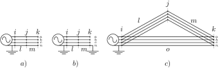
In networks where each continuous neutral section is grounded only once (e.g. Fig. 2a, Fig. 2c), the algorithm’s solution is not only unique, but also identical to that of the original 4x4 Ohm’s law (5) problem! The reason is that KCL is satisfied everywhere, and only the single grounding allows the neutral current to flow. The neutral current therefore must be uniquely determined through the inductive coupling with the phases, and the current balance w.r.t loads/generators. When the network is grounded on multiple locations, the current will divide across the different paths to ground, and therefore the constraint (16) is needed to guarantee the correct solution.

2.5. Discussion

Note that the load behavior (8) is still valid, and generalizes to ZIP and exponential load models. KCL (6) only requires the phase-currents now. We refer to (Geth et al., 2020) for a comprehensive description of the feasible set of 3-wire (O)PF.

The proposed phase-to-neutral impedance transformation is exact when the following conditions hold simultaneously:

  1. (1)

    networks with branches without shunt admittance between the conductors and earth;

  2. (2)

    networks where none of the connected devices put current into the ground;

  3. (3)

    networks where neutral grounding is only performed once for each continuous neutral section.

In any other circumstance, it is either a true approximation, a relaxation, or both. The three conditions are realistic assumptions in single-grounded LV networks. However, at higher voltage levels, and/or in multi-grounded systems, the assumptions are harder to justify. Therefore in the next section we will perform numerical experiments to understand the implications.

In the context of optimization problems, by performing the transformation, we have eliminated the bus neutral voltage and line neutral current variables, thereby reducing the problem size significantly. In post-processing, we run Algorithm 1 to recover the neutral voltage values. We can now directly impose magnitude bounds on the phase-to-neutral voltages, however, we lose the ability to impose neutral-to-ground voltage limits444that would require adding neutral voltage variables and (16).. Neutral current limits are still enforcable using (10),

(17) $$|{\color[rgb]{0,0,1}I_{{l}{i}{j},{n}}}|\rightarrow|{\color[rgb]{0,0,1}I_{{l}{i}{j},{a}}}+{\color[rgb]{0,0,1}I_{{l}{i}{j},{b}}}+{\color[rgb]{0,0,1}I_{{l}{i}{j},{c}}}|\leq{\color[rgb]{1,0,0}I_{l,n}^{\text{max}}}.$$

Note that we do not suggest this transformation technique should be used in simulation contexts without justification, despite high accuracy in contexts that may be easy to identify a-priori. As Kersting writes in his seminal book (Kersting, 2001)When the [simulation] analysis is being done using a computer, the approach to take is to go ahead and model the shunt admittance for both overhead and underground lines. Why make a simplifying assumption when it is not necessary?”. The scalability of power flow solvers using for example the fixed-point iteration variant of the current injection method is vastly better than the scalability of nonlinear unbalanced optimal power flow (UBOPF). Therefore, the impedance transformation approach can be justified more easily for UBOPF.

2.6. Contrast: Kron’s Reduction of the Neutral

To enable the computational comparison between different impedance transformations in the upcoming section, we now briefly summarize Kron’s reduction of the neutral. Kron’s reduction of the neutral is defined for a partition of the series impedance matrix based on the neutral self-impedance,

(18) $${\color[rgb]{.75,.5,.25}\mathbf{z}_{{l}}^{\text{{s}}}}=\left[\begin{array}[]{c|c}{\color[rgb]{.75,.5,.25}\mathbf{z}^{\text{PP}}_{l}}&{\color[rgb]{.75,.5,.25}\mathbf{z}^{\text{PN}}_{l}}\\ \hline\cr{\color[rgb]{.75,.5,.25}\mathbf{z}^{\text{NP}}_{l}}&{\color[rgb]{.75,.5,.25}z_{{l},{n}{n}}^{\text{{s}}}}\end{array}\right]\in{\color[rgb]{.25,.25,.25}\mathbb{C}}^{4\times 4},{\color[rgb]{.75,.5,.25}\mathbf{z}^{\text{PP}}_{l}}\in{\color[rgb]{.25,.25,.25}\mathbb{C}}^{3\times 3},{\color[rgb]{.75,.5,.25}\mathbf{z}^{\text{PN}}_{l}},({\color[rgb]{.75,.5,.25}\mathbf{z}^{\text{NP}}_{l}})^{\text{T}}\in{\color[rgb]{.25,.25,.25}\mathbb{C}}^{3\times 1}.$$

We also partition Ohm’s law (5) accordingly,

(19) $$\left[\begin{array}[]{c}{\color[rgb]{0,0,1}\mathbf{U}_{{j}}}[{\color[rgb]{1,0,0}\mathcal{P}}]\\ \hline\cr{\color[rgb]{0,0,1}U_{{j},{n}}}\end{array}\right]=\left[\begin{array}[]{c}{\color[rgb]{0,0,1}\mathbf{U}_{{i}}}[{\color[rgb]{1,0,0}\mathcal{P}}]\\ \hline\cr{\color[rgb]{0,0,1}U_{{i},{n}}}\end{array}\right]-\left[\begin{array}[]{c|c}{\color[rgb]{.75,.5,.25}\mathbf{z}^{\text{PP}}_{l}}&{\color[rgb]{.75,.5,.25}\mathbf{z}^{\text{PN}}_{l}}\\ \hline\cr{\color[rgb]{.75,.5,.25}\mathbf{z}^{\text{NP}}_{l}}&{\color[rgb]{.75,.5,.25}z_{{l},{n}{n}}^{\text{{s}}}}\end{array}\right]\left[\begin{array}[]{c}{\color[rgb]{0,0,1}\mathbf{I}_{{l}{i}{j}}^{\text{{s}}}}[{\color[rgb]{1,0,0}\mathcal{P}}]\\ \hline\cr{\color[rgb]{0,0,1}I_{{l}{i}{j},{n}}^{\text{{s}}}}\end{array}\right].$$

Under the assumption ${\color[rgb]{0,0,1}U_{{i},{n}}}\approx 0\approx{\color[rgb]{0,0,1}U_{{j},{n}}}$ we derive an expression for the neutral current from the lower entries of (19):

(20) $${\color[rgb]{0,0,1}I_{{l}{i}{j},{n}}^{\text{{s}}}}=-\frac{1}{{\color[rgb]{.75,.5,.25}z_{{l},{n}{n}}^{\text{{s}}}}}{\color[rgb]{.75,.5,.25}\mathbf{z}^{\text{NP}}_{l}}{\color[rgb]{0,0,1}\mathbf{I}_{{l}{i}{j}}^{\text{{s}}}}[{\color[rgb]{1,0,0}\mathcal{P}}].$$

We substitute this in the top entries of (19) and obtain,

(21) $${\color[rgb]{0,0,1}\mathbf{U}_{{j}}}[{\color[rgb]{1,0,0}\mathcal{P}}]={\color[rgb]{0,0,1}\mathbf{U}_{{i}}}[{\color[rgb]{1,0,0}\mathcal{P}}]-\left({\color[rgb]{.75,.5,.25}\mathbf{z}^{\text{PP}}_{l}}-\frac{1}{{\color[rgb]{.75,.5,.25}z_{{l},{n}{n}}^{\text{{s}}}}}{\color[rgb]{.75,.5,.25}\mathbf{z}^{\text{PN}}_{l}}{\color[rgb]{.75,.5,.25}\mathbf{z}^{\text{NP}}_{l}}\right){\color[rgb]{0,0,1}\mathbf{I}_{{l}{i}{j}}^{\text{{s}}}}[{\color[rgb]{1,0,0}\mathcal{P}}].$$

Kron’s reduction of the neutral is now defined as the transformation $\mathcal{K}$,

(22) $$\mathcal{K}({\color[rgb]{.75,.5,.25}\mathbf{z}_{{l}}^{\text{{s}}}})={\color[rgb]{.75,.5,.25}\mathbf{z}^{\text{PP}}_{l}}-\frac{1}{{\color[rgb]{.75,.5,.25}z_{{l},{n}{n}}^{\text{{s}}}}}{\color[rgb]{.75,.5,.25}\mathbf{z}^{\text{PN}}_{l}}{\color[rgb]{.75,.5,.25}\mathbf{z}^{\text{NP}}_{l}}.$$

Note that this transformation is nonlinear in the entries of ${\color[rgb]{.75,.5,.25}\mathbf{z}_{{l}}^{\text{{s}}}}$; for further details we refer the reader to (Dorfler and Bullo, 2013). For completeness, we provide the corresponding transformation for the shunt admittance in the $\Pi$-section,

(23) $$\left[\begin{array}[]{c}{\color[rgb]{0,0,1}\mathbf{I}_{{l}{i}{j}}^{\text{{sh}}}}[{\color[rgb]{1,0,0}\mathcal{P}}]\\ \hline\cr{\color[rgb]{0,0,1}I_{{l}{i}{j},{n}}^{\text{{sh}}}}\end{array}\right]=\left[\begin{array}[]{c|c}{\color[rgb]{.75,.5,.25}\mathbf{y}^{\text{PP}}_{l}}&{\color[rgb]{.75,.5,.25}\mathbf{y}^{\text{PN}}_{l}}\\ \hline\cr{\color[rgb]{.75,.5,.25}\mathbf{y}^{\text{NP}}_{l}}&{\color[rgb]{.75,.5,.25}y_{{l}{i}{j},{n}{n}}^{\text{{sh}}}}\end{array}\right]\left[\begin{array}[]{c}{\color[rgb]{0,0,1}\mathbf{U}_{{i}}}[{\color[rgb]{1,0,0}\mathcal{P}}]\\ \hline\cr{\color[rgb]{0,0,1}U_{{i},{n}}}\approx 0\end{array}\right],$$

which tells us the neutral shunt current is ${\color[rgb]{0,0,1}I_{{l}{i}{j},{n}}^{\text{{sh}}}}={\color[rgb]{.75,.5,.25}\mathbf{y}^{\text{NP}}_{l}}{\color[rgb]{0,0,1}\mathbf{U}_{{i}}}[{\color[rgb]{1,0,0}\mathcal{P}}]$.

Whereas Kron’s reduction of the neutral assumes the neutral is perfectly grounded everywhere (${\color[rgb]{0,0,1}U_{{i},{n}}}=0\,\forall i$), the phase-to-neutral transform allows the neutral voltage to be nonzero everywhere, except for a limited set of buses. Both transformations generate $3\times 3$ impedance matrices, with voltage variables after the transformation to be interpreted as phase-to-neutral voltages.

3. Numerical experiments

Table 2 summarizes the formulations discussed in the previous sections. These transformations will be compared numerically in this section.

Table 2. Summary of Impedance Transformations
Transform Result Assumptions
$\mathcal{O}$ Original (do-nothing) $4\times 4$ -
$\mathcal{K}$ Kron’s reduction $3\times 3$ neutral voltage 0
$\mathcal{T}$ Phase-to-neutral (proposed) $3\times 3$ ground current 0
$\mathcal{U}$ Modified phase-to-neutral $3\times 3$ ground current 0,
no mutual impedance

3.1. Data Sets

We have adapted a previously-developed library of 128 single-grounded networks (Claeys, 2021), based on originals from the Low-Voltage Network Solutions project (LVN, 2014).

  • explicit-neutral versions of ‘ENWL’ networks (LVN, 2014) with impedance data replaced with data developed by Urquhart and Thomson (Urquhart and Thomson, 2015) ($\mathcal{O}$, $4\times 4$);

  • the Kron-reduced equivalents ($\mathcal{K},3\times 3$, previously explored in (Claeys, 2021));

  • novel phase-to-neutral transformed versions ($\mathcal{T},3\times 3$);

  • novel modified phase-to-neutral transformed versions ($\mathcal{U},3\times 3$).

Note that these networks start at the 11 kV bus, and then include a delta-grounded-wye transformer, providing the sink for the neutral current. Each of these test cases have only a single neutral grounding, and are lacking shunt admittance data, and therefore are expected to be exact under the phase-to-neutral transformation. Note that all this networks exclusively contain cables, not overhead lines.

Moreover, we include a simple 4-wire overhead line MV 2-bus single-grounded validation system from Kersting and Philips (Kersting and Philips, 1995). This example includes shunt admittance data, and different levels of load unbalance, and therefore serves as a good sensitivity study. Finally, we also develop a similar 2-bus single-grounded system for an Australian LV overhead line.

3.2. Software

We use OpenDSS (Dugan and McDermott, 2011) as a well-tested unbalanced power flow solver that supports explicit neutral wires. We apply the proposed transformation to the OpenDSS data and write it to a new file, and compare the voltages and currents w.r.t. the originals. The Julia toolbox PowerModelsDistribution (PMD) (Fobes et al., 2020) is used to build the UBOPF problems. As PMD has a built-in OpenDSS parser, we also generate the transformed ‘DSS’ files for the different transformations (Table 2), allowing us to validate w.r.t OpenDSS as well as to solve UBOPF case studies.

PMD contains high-quality implementations of the 3-wire (detailed in (Geth et al., 2020)) and 4-wire UBOPF models (detailed in (Claeys et al., 2022)). These implementations are consistent with seminal work (Araujo et al., 2013). We specifically use the rectangular current-voltage formulation, which results in nonconvex quadratic programming models, that are solved through JuMP (Dunning et al., 2017) (for automatic differentiation) and Ipopt (Wächter and Biegler, 2006) (nonlinear programming solver). In our experience, voltage variable initialization is crucial for reliability and convergence speed, however it is not as crucial for the other variables (current, power). Therefore in our experiments, the voltage variables are initialized at a balanced 1-pu phasor, with the neutral voltage set to 0 (where applicable). Note that when traversing transformers, those initialized voltage phasors are rotated according to the transformer vector group.

We configure both OpenDSS and Ipopt to a numerical tolerance of 1E-8.

3.3. Validation and Approximation Error

In this section, we compare power flow results between the original 4-wire data and the phase-to neutral transform. First, we compare cases without shunts to ground, to serve as validation. Secondly, we compare 4-wire cases with nonzero shunt admittance, to understand the impact of neglecting the shunts when doing the phase-to-neutral transformation.

3.3.1. Line Shunts Negligible

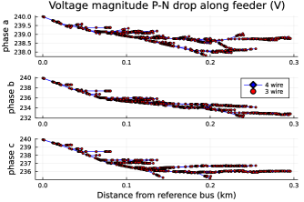
Fig. 3 shows phase to neutral voltage magnitude drop along a feeder (specifically network 1 feeder 1) of one of the ENWL test cases for both 4-wire $\mathcal{O}$ and 3-wire $\mathcal{T}$. We see that all values match.

Refer to caption
Figure 3. Comparison of original and phase-to-neutral impedance models on voltage magnitudes along the feeder 1 of network 1 (906 buses. The 4-wire $\mathcal{O}$ and 3-wire $\mathcal{T}$ voltages overlap in all three phases across the network).

We note that the voltages are identical to numerical tolerance for the phase-to-neutral transformation across all 128 networks.
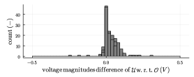
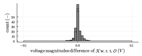
Figures 45 depict the voltage magnitude difference for the modified phase-to-neutral transformation $\mathcal{U}$ and Kron’s reduction $\mathcal{K}$. It is noted that $\mathcal{U}$ is the least accurate and that $\mathcal{K}$ has small, but non-zero difference.

Refer to caption
Figure 4. Histogram depicting voltage magnitudes difference of the modified phase-to-neutral transformation $\mathcal{U}$ across the library of 128 networks.
Refer to caption
Figure 5. Histogram depicting voltage magnitudes difference of the Kron’s reduction $\mathcal{K}$ across the library of 128 networks.

3.3.2. Line Shunts Nonnegligible

The goal here is to understand the transformation where it is a true approximation - i.e. cases with shunt admittance. We compare two 2-bus single-grounded overhead-line cases: a MV one previously published by Kersting, and a novel one, based on a common Australian LV overhead line configuration. The source bus has a fixed, balanced voltage phasor with grounded neutral, the second bus has a constant power load with ungrounded neutral. We analyse three scenarios for the load: balanced, unbalanced and very unbalanced. Note that, due to the detailed impedance models used, even with a balanced load, the current/voltage phasors aren’t balanced, as the line impedance isn’t balanced. Table 3 reports the power flow results for the simple 4-wire 12.47 $kV$ system described in Kersting (Kersting and Philips, 1995) with nonnegligible line shunts. Comparison of the phase-to-neutral voltage magnitudes show that the $\mathcal{T}$ has a small difference with respect to the original 4-wire line model, despite the nonnegligible line shunt.

Table 3. Power flow results Kersting: voltage magnitudes and comparisons. Balanced, unbalanced, and very unbalanced load setpoints are respectively: [3, 3, 3] MVA, [4, 3, 2] MVA, and [4, 0.3, 2] MVA, PF 0.9 lagging.
Model $|{\color[rgb]{0,0,1}U_{{i},{a}{n}}}|$ $|{\color[rgb]{0,0,1}U_{{i},{b}{n}}}|$ $|{\color[rgb]{0,0,1}U_{{i},{c}{n}}}|$
$\mathcal{O}$ bal. 0.93241815 0.96099983 0.94272734 (pu)
unb. 0.85158645 1.00804238 0.98165957 (pu)
very unb. 0.87569142 1.09761676 0.92216782 (pu)
$\mathcal{T}$ bal. 0.93241001 0.96099242 0.94272011 (pu)
unb. 0.85157804 1.00803523 0.98165219 (pu)
very unb. 0.87568319 1.09760949 0.92216047 (pu)
$\mathcal{U}$ bal. 0.87975849 0.87975849 0.87975849 (pu)
unb. 0.73327937 0.9535492 0.9783037 (pu)
very unb. 0.56748513 1.20372151 0.93725998 (pu)
$\mathcal{K}$ bal. 0.93270236 0.95880124 0.94469055 (pu)
unb. 0.88275064 0.98653945 0.97183049 (pu)
very unb. 0.90210055 1.05734142 0.93567207 (pu)
$\mathcal{T}$ - $\mathcal{O}$ bal. -8E-06 -7E-06 -7E-06 (pu)
unb. -8E-06 -7E-06 -7E-06 (pu)
very unb. -8E-06 -7E-06 -7E-06 (pu)
$\mathcal{U}$ - $\mathcal{O}$ bal. -0.05266 -0.081241 -0.062969 (pu)
unb. -0.118307 -0.054493 -0.003356 (pu)
very unb. -0.308206 0.106105 0.015092 (pu)
$\mathcal{K}$ - $\mathcal{O}$ bal. 0.000284 -0.002199 0.001963 (pu)
unb. 0.031164 -0.021503 -0.009829 (pu)
very unb. 0.026409 -0.040275 0.013504 (pu)

A similar analysis has been carried out for an Australian distribution two-bus system with an overhead line (modeled from Carson’s equations), and the results are reported in Table 4.

Table 4. Power flow results Australian overhead line: voltage magnitudes and comparisons. Balanced, unbalanced, and very unbalanced load setpoints are respectively: [30, 30, 30] kVA, [40, 30, 20] kVA, and [40, 3, 20] kVA, PF 0.9 lagging.
Model $|{\color[rgb]{0,0,1}U_{{i},{a}{n}}}|$ $|{\color[rgb]{0,0,1}U_{{i},{b}{n}}}|$ $|{\color[rgb]{0,0,1}U_{{i},{c}{n}}}|$
$\mathcal{O}$ bal. 0.94692051 0.97494785 0.96777093 (pu)
unb. 0.89880375 1.00170312 0.99102676 (pu)
very unb. 0.91174448 1.06698015 0.95470596 (pu)
$\mathcal{T}$ bal. 0.94691995 0.97494315 0.96777538 (pu)
unb. 0.89881128 1.0016897 0.99103186 (pu)
very unb. 0.91175119 1.06697602 0.95470524 (pu)
$\mathcal{U}$ bal. 0.92496348 0.92496348 0.92496348 (pu)
unb. 0.79688733 0.99131649 0.98129524 (pu)
very unb. 0.82994038 1.1092935 0.90006353 (pu)
$\mathcal{K}$ bal. 0.95221817 0.97128645 0.96623487 (pu)
unb. 0.92136173 0.98786491 0.98295279 (pu)
very unb. 0.93358972 1.03739209 0.95948488 (pu)
$\mathcal{T}$ - $\mathcal{O}$ bal. -1.00E-06 -5.00E-06 4.00E-06 (pu)
unb. 8.00E-06 -1.30E-05 5.00E-06 (pu)
very unb. 7.00E-06 -4.00E-06 -1.00E-06 (pu)
$\mathcal{U}$ - $\mathcal{O}$ bal. -0.021957 -0.049984 -0.042807 (pu)
unb. -0.101916 -0.010387 -0.009732 (pu)
very unb. -0.081804 0.042313 -0.054642 (pu)
$\mathcal{K}$ - $\mathcal{O}$ bal. 0.005298 -0.003661 -0.001536 (pu)
unb. 0.022558 -0.013838 -0.008074 (pu)
very unb. 0.021845 -0.029588 0.004779 (pu)

We conclude that for both cases, the error due to neglecting the shunts and then doing the phase-to-neutral transformation is small. Transformation $\mathcal{U}$ should be avoided in MV, as the mutual impedance values are significant. The phase-to-neutral transformation is the best $3\times 3$ representation overall - for these cases with a single-grounded neutral. If both buses would have a grounded neutral, Kron’s reduction would be the best.

3.4. Scalability in UBOPF

OpenDSS files describe power flow simulation case studies, not UBOPF ones. To use these network case studies as UBOPF examples we therefore now add bounds and degrees of freedom.

3.4.1. Adding Voltage Bounds and Generators

The voltage magnitude bounds are set to

(24) $$\begin{bmatrix}0.9pu\\ 0.9pu\\ 0.9pu\\ \end{bmatrix}=\begin{bmatrix}{\color[rgb]{1,0,0}U_{{i},{a}{n}}^{\text{min}}}\\ {\color[rgb]{1,0,0}U_{{i},{b}{n}}^{\text{min}}}\\ {\color[rgb]{1,0,0}U_{{i},{c}{n}}^{\text{min}}}\\ \end{bmatrix}\leq\begin{bmatrix}|{\color[rgb]{0,0,1}U_{{i},{a}{n}}}|\\ |{\color[rgb]{0,0,1}U_{{i},{b}{n}}}|\\ |{\color[rgb]{0,0,1}U_{{i},{c}{n}}}|\end{bmatrix}\leq\begin{bmatrix}{\color[rgb]{1,0,0}U_{{i},{a}{n}}^{\text{max}}}\\ {\color[rgb]{1,0,0}U_{{i},{b}{n}}^{\text{max}}}\\ {\color[rgb]{1,0,0}U_{{i},{c}{n}}^{\text{max}}}\\ \end{bmatrix}=\begin{bmatrix}1.1pu\\ 1.1pu\\ 1.1pu\\ \end{bmatrix}.$$

Note that in the four-wire case, the phase-to-ground voltages are still bounded. However, for the purposes of formal formulation of an optimisation problem, these bounds are weakly expressed at values that cannot become binding before the phase-to-neutral limits, even at maximal neutral voltage shift (i.e. ¿1.1pu). We fix the voltage phasor at the reference bus,

(25) $${\color[rgb]{0,0,1}\mathbf{U}_{{i}}}=\begin{bmatrix}{\color[rgb]{.75,.5,.25}U_{{i},{a}}^{\text{ref}}}\\ {\color[rgb]{.75,.5,.25}U_{{i},{b}}^{\text{ref}}}\\ {\color[rgb]{.75,.5,.25}U_{{i},{c}}^{\text{ref}}}\\ {\color[rgb]{.75,.5,.25}U_{{i},n}^{\text{ref}}}\\ \end{bmatrix}=\begin{bmatrix}1{\color[rgb]{1,0,0}\angle}0^{\circ}pu\\ 1{\color[rgb]{1,0,0}\angle}-120^{\circ}pu\\ 1{\color[rgb]{1,0,0}\angle}120^{\circ}pu\\ 0pu\end{bmatrix}.$$

We read in the 128 networks, add a slack generator to represent the external system (capable of absorbing power if needed), and then add a distributed generator (DG) to the bus of each fourth load555Load IDs are numbers in the original data.. The objective is to minimize the total generation cost. Each DG has the same cost, but the slack generator is twice as expensive. Therefore, we expect the DGs to be dispatched until the voltage limits become binding. Note that due to losses in the power flow, and up to one generator per bus, the solution is not degenerate despite identical costs, as the influence of the generators on the network losses will be different. Note that for a few test cases, Ipopt did not converge for the modified phase-to-neutral transformation (the others transformations did not pose problems), therefore we removed those from the UBOPF testing, ending up with a final set of 111 networks.

3.4.2. Computation Speed Results

Fig. 6 depicts the ratio of computation time of the 4-wire case studies before and after the phase-to-neutral transformation. Most cases have a speedup above 1, therefore we conclude an overall improvement. The mean speedup is 1.42 with 25 cases solving slower than the 4-wire original.

Refer to caption
Figure 6. Histogram depicting the computational speedup of the phase-to-neutral transformation $\mathcal{T}$ across 111 networks.

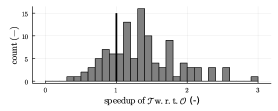
Fig. 7 depicts the ratio of computation time of the 4-wire case studies before and after the modified phase-to-neutral transformation. The mean speedup is 1.37 with 29 cases solving slower than the 4-wire original.

Refer to caption
Figure 7. Histogram depicting the computational speedup of the modified phase-to-neutral transformation $\mathcal{U}$ across 111 networks.

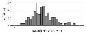
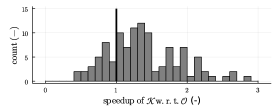
Fig.8 depicts the ratio of computation time of the 4-wire case studies before and after Kron’s reduction. The mean speedup is 1.43 with 24 cases solving slower than the 4-wire original.

Refer to caption
Figure 8. Histogram depicting the computational speedup of Kron’s reduction $\mathcal{K}$ across 111 networks.

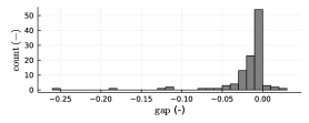
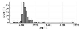
The modified phase-to-neutral transformation and Kron’s reduction result in different dispatch decisions and therefore optimal objective values. We quantify the gap for the former in Fig. 9 and the latter in Fig. 10. We note that the gap with Kron’s reduction is typically small, however, it is nonzero. Therefore, the phase-to-neutral transformation should be considered preferentially in single-grounded networks.

Refer to caption
Figure 9. Histogram depicting optimality gap of the modified phase-to-neutral transformation $\mathcal{U}$ across the 111 networks.
Refer to caption
Figure 10. Histogram depicting optimality gap of Kron’s reduction $\mathcal{K}$ across the 111 networks.

We note that the scalability improvements of the proposed transformation are nice-to-have, as part of set of techniques available to practitioners looking to stretch performance. Nevertheless, it is not game-changing, as we are still bound by the limitations of interior-point methods for nonlinear programming.

3.4.3. Discussion

Note that in the four-wire context phase-to-neutral voltage bounds require an explicit phase-to-neutral variable and constraint for each phase (4), or the following quadratic expression in phase-to-ground variables:
$\begin{bmatrix}{\color[rgb]{1,0,0}U_{{i},{a}{n}}^{\text{min}}}\\ {\color[rgb]{1,0,0}U_{{i},{b}{n}}^{\text{min}}}\\ {\color[rgb]{1,0,0}U_{{i},{c}{n}}^{\text{min}}}\\ \end{bmatrix}\leq\begin{bmatrix}({\color[rgb]{0,0,0}U_{{i},{a}}^{\text{re}}})^{2}+({\color[rgb]{0,0,0}U_{{i},{a}}^{\text{im}}})^{2}+({\color[rgb]{0,0,0}U_{{i},{n}}^{\text{re}}})^{2}+({\color[rgb]{0,0,0}U_{{i},{n}}^{\text{im}}})^{2}-2{\color[rgb]{0,0,0}U_{{i},{a}}^{\text{re}}}{\color[rgb]{0,0,0}U_{{i},{n}}^{\text{re}}}+2{\color[rgb]{0,0,0}U_{{i},{a}}^{\text{im}}}{\color[rgb]{0,0,0}U_{{i},{n}}^{\text{im}}}\\ ({\color[rgb]{0,0,0}U_{{i},{b}}^{\text{re}}})^{2}+({\color[rgb]{0,0,0}U_{{i},{b}}^{\text{im}}})^{2}+({\color[rgb]{0,0,0}U_{{i},{n}}^{\text{re}}})^{2}+({\color[rgb]{0,0,0}U_{{i},{n}}^{\text{im}}})^{2}-2{\color[rgb]{0,0,0}U_{{i},{b}}^{\text{re}}}{\color[rgb]{0,0,0}U_{{i},{n}}^{\text{re}}}+2{\color[rgb]{0,0,0}U_{{i},{b}}^{\text{im}}}{\color[rgb]{0,0,0}U_{{i},{n}}^{\text{im}}}\\ ({\color[rgb]{0,0,0}U_{{i},{c}}^{\text{re}}})^{2}+({\color[rgb]{0,0,0}U_{{i},{c}}^{\text{im}}})^{2}+({\color[rgb]{0,0,0}U_{{i},{n}}^{\text{re}}})^{2}+({\color[rgb]{0,0,0}U_{{i},{n}}^{\text{im}}})^{2}-2{\color[rgb]{0,0,0}U_{{i},{c}}^{\text{re}}}{\color[rgb]{0,0,0}U_{{i},{n}}^{\text{re}}}+2{\color[rgb]{0,0,0}U_{{i},{c}}^{\text{im}}}{\color[rgb]{0,0,0}U_{{i},{n}}^{\text{im}}}\\ \end{bmatrix}\leq\begin{bmatrix}{\color[rgb]{1,0,0}U_{{i},{a}{n}}^{\text{max}}}\\ {\color[rgb]{1,0,0}U_{{i},{b}{n}}^{\text{max}}}\\ {\color[rgb]{1,0,0}U_{{i},{c}{n}}^{\text{max}}}\\ \end{bmatrix}.$

(26)

The phase-to-neutral transform $\mathcal{T}$ has results in more simple expressions, as it is defined in phase-to-neutral variables,

(27) $$\begin{bmatrix}{\color[rgb]{1,0,0}U_{{i},{a}{n}}^{\text{min}}}\\ {\color[rgb]{1,0,0}U_{{i},{b}{n}}^{\text{min}}}\\ {\color[rgb]{1,0,0}U_{{i},{c}{n}}^{\text{min}}}\\ \end{bmatrix}\leq\begin{bmatrix}({\color[rgb]{0,0,0}U_{{i},{a}{n}}^{\text{re}}})^{2}+({\color[rgb]{0,0,0}U_{{i},{a}}^{\text{im}}})^{2}\\ ({\color[rgb]{0,0,0}U_{{i},{b}{n}}^{\text{re}}})^{2}+({\color[rgb]{0,0,0}U_{{i},{b}}^{\text{im}}})^{2}\\ ({\color[rgb]{0,0,0}U_{{i},{c}{n}}^{\text{re}}})^{2}+({\color[rgb]{0,0,0}U_{{i},{c}}^{\text{im}}})^{2}\\ \end{bmatrix}\leq\begin{bmatrix}{\color[rgb]{1,0,0}U_{{i},{a}{n}}^{\text{max}}}\\ {\color[rgb]{1,0,0}U_{{i},{b}{n}}^{\text{max}}}\\ {\color[rgb]{1,0,0}U_{{i},{c}{n}}^{\text{max}}}\\ \end{bmatrix}.$$

We believe the improvement in computation speed can be partially explained by the simpler expressions for the voltage magnitude bounds. Nevertheless, the availability of diverse benchmarks for UBOPF is still problematic, so the computational speedup may not be as significant with different network configurations.

4. Conclusions

Similar to Kron’s reduction, the proposed phase-to-neutral transformation reduces the size of the line matrices from $4\times 4$ to $3\times 3$, and can be solved with 3 voltage variables per bus instead of 4. The novel transformation has properties which are distinct from Kron’s reduction though:

  • it can facilitate some, but only a few, buses with neutral grounded, versus requiring the neutral at all buses to be grounded;

  • establishes neutral voltage shift, instead of approximating it as 0.

When the shunt current induced in the ground is negligible throughout the network except for at one bus where grounding enables current to flow into the ground, this work shows that you can uniquely recover the neutral voltage rise without needing explicit neutral voltage variables. In MV networks, or in sparsely-grounded networks, the transformation may still provide a high-quality approximation that offers computational benefits. We believe the proposed transformation is fundamentally superior to Kron’s reduction for single-grounded MV and LV networks, due to inherently limited branch shunt current contributions to the power flow at those voltage levels and due to the ability to capture neutral voltage shift accurately. Furthermore, the computation speed of the proposed transformation is slightly better than that of Kron’s reduction and the original 4-wire description.

Throughout the development of this paper, the authors noted a lack of network data sets that are 1) explicitly four-wire, 2) with unbalanced impedance matrices, 3) with line shunt data, 4) with complete neutral grounding descriptions. Often the data sets 1) are missing shunt admittance values, 2) assume balanced series impedances (e.g. because defined in terms of positive and zero sequence impedance only), 3) are only available in Kron-reduced form.

Future work therefore includes 1) the development of unbalanced OPF data model and data sets, specifically with multiple neutral grounding setups; 2) broader comparison of impedance transformations and coordinate spaces (e.g. sequence components). Finally, we conjecture an application where the proposed transformation may improve algorithmic scalability more impressively. For four-wire UBOPF in the power-voltage variable space, the neutral voltage does not have a magnitude lower bound, which causes convergence issues in nonlinear programming (due to $S=UI^{*}$ where $U\approx 0$) (Claeys et al., 2022). With the proposed transformation, one does not need explicit neutral voltage variables, thereby likely enabling more reliable solving of the power-voltage equations.

Acknowledgements.
The authors are grateful to Sander Claeys for doing a lot of the ground work preparing the test cases. We also appreciate Andrew Urquhart and Murray Thomson’s help in the generation of the impedance data (Urquhart and Thomson, 2015) for the test case library. Finally, the authors are grateful to all the contributors to the open source packages that enabled this work, including but not limited to JuMP (Dunning et al., 2017), Ipopt (Wächter and Biegler, 2006), PowerModelsDistribution(Fobes et al., 2020).

References

  • (1)
  • LVN (2014) 2014. Low voltage network solutions closedown report. Technical Report June. Low Carbon Networks Fund. 74 pages. https://www.ofgem.gov.uk/sites/default/files/docs/2017/04/lvns_closedown_report.pdf.
  • Araujo et al. (2013) Leandro Ramos De Araujo, Débora Rosana Ribeiro Penido, and Felipe De Alcântara Vieira. 2013. A multiphase optimal power flow algorithm for unbalanced distribution systems. Int. J. Elec. Power Energy Syst. 53, 1 (2013), 632–642. https://doi.org/10.1016/j.ijepes.2013.05.028
  • Ciric et al. (2003) Rade M Ciric, Antonio Padilha Feltrin, and Luis F Ochoa. 2003. Power flow in four-wire distribution networks - general approach. IEEE Trans. Power Syst. 18, 4 (2003), 1283–1290.
  • Claeys (2021) Sander Claeys. 2021. Distribution network modeling: from simulation towards optimization. PhD Dissertation. KU Leuven.
  • Claeys et al. (2022) Sander Claeys, Frederik Geth, and Geert Deconinck. 2022. Optimal power flow in four-wire distribution networks: formulation and benchmarking. In accepted for Power Systems Computation Conference. Porto, Portugal, 1–8.
  • Claeys et al. (2021) Sander Claeys, Marta Vanin, Frederik Geth, and Geert Deconinck. 2021. Applications of optimization models for electricity distribution networks. Wiley Interdisciplinary Reviews: Energy and Environment (2021), e401.
  • Dorfler and Bullo (2013) Florian Dorfler and Francesco Bullo. 2013. Kron reduction of graphs with applications to electrical networks. IEEE Trans. Circuits Systems I: Regular Papers 60, 1 (feb 2013), 1–28.
  • Dugan and McDermott (2011) Roger C. Dugan and Thomas E. McDermott. 2011. An open source platform for collaborating on smart grid research. IEEE Power Energy Soc. General Meeting (2011), 1–7. https://doi.org/10.1109/PES.2011.6039829
  • Dunning et al. (2017) Iain Dunning, Joey Huchette, and Miles Lubin. 2017. JuMP: a modeling language for mathematical optimization. SIAM Rev. 59, 2 (2017), 295–320. https://doi.org/10.1137/15M1020575
  • Fobes et al. (2020) David M Fobes, Carleton Coffrin, Frederik Geth, and Sander Claeys. 2020. PowerModelsDistribution. jl: an open-source framework for exploring distribution power flow formulations. Electric Power Systems Research 189, December (2020), 106664.
  • Geth et al. (2020) Frederik Geth, Sander Claeys, and Geert Deconinck. 2020. Current-voltage formulation of the unbalanced optimal power flow problem. In 8th Workshop Model. Simulation Cyber-Phys. Energy Syst. Sydney, Australia, 1–6.
  • Kersting and Philips (1995) W.H. Kersting and W. H. Philips. 1995. Distribution feeder line models. IEEE Trans. Ind. Appl. 31, 4 (1995), 715–720.
  • Kersting (2001) William H. Kersting. 2001. Distribution system modeling and analysis. 1–314 pages. https://doi.org/10.1201/9781315222424-27
  • Koirala et al. (2019) Arpan Koirala, Reinhilde D’hulst, and Dirk Van Hertem. 2019. Impedance modelling for European style distribution feeder. 2019 International Conference on Smart Energy Systems and Technologies (SEST) (2019), 1–6. https://doi.org/10.1109/sest.2019.8849015
  • Olivier et al. (2018) Frédéric Olivier, R. Fonteneau, and Damien Ernst. 2018. Modelling of three-phase four-wire low-voltage cables taking into account the neutral connection to the earth. In CIRED workshop. Ljubljana, 1–4.
  • Urquhart and Thomson (2015) Andrew J. Urquhart and Murray Thomson. 2015. Series impedance of distribution cables with sector-shaped conductors. IET Gener. Transm. Distrib. 9, 16 (2015), 2679–2685. https://doi.org/10.1049/iet-gtd.2015.0546
  • Wächter and Biegler (2006) Andreas Wächter and Lorenz T. Biegler. 2006. On the implementation of primal-dual interior point filter line search algorithm for large-scale nonlinear programming. Math. Prog. 106, 1 (2006), 25–57. https://doi.org/10.1007/s10107-004-0559-y

Appendix A Appendix: Reduced Phases

In this section we illustrate how the phase-to-neutral transformation works in a single-phase branch, as these are relatively common in practice. We perform the transformation for a two-wire branch with phase $a$ and neutral $n$. Ohm’s law now uses a $2\times 2$ matrix,

(28) $$\begin{bmatrix}{\color[rgb]{0,0,1}U_{{i},{a}}}\\ {\color[rgb]{0,0,1}U_{{i},{n}}}\end{bmatrix}=\begin{bmatrix}{\color[rgb]{0,0,1}U_{{j},{a}}}\\ {\color[rgb]{0,0,1}U_{{j},{n}}}\end{bmatrix}-\underbrace{\begin{bmatrix}{\color[rgb]{.75,.5,.25}z_{{l},{a}{a}}^{\text{{s}}}}&{\color[rgb]{.75,.5,.25}z_{{l},{a}{n}}^{\text{{s}}}}\\ {\color[rgb]{.75,.5,.25}z_{{l},{n}{a}}^{\text{{s}}}}&{\color[rgb]{.75,.5,.25}z_{{l},{n}{n}}^{\text{{s}}}}\\ \end{bmatrix}}_{{\color[rgb]{.75,.5,.25}\mathbf{z}_{{l}}^{\text{{s}}}}}\begin{bmatrix}{\color[rgb]{0,0,1}I_{{l}{i}{j},{a}}}\\ {\color[rgb]{0,0,1}I_{{l}{i}{j},{n}}}\end{bmatrix}.$$

The phase-to-neutral voltage is,

(29) $${\color[rgb]{0,0,1}U_{{i},{a}{n}}}=\underbrace{\begin{bmatrix}1&-1\\ \end{bmatrix}}_{{\color[rgb]{1,0,0}\mathbf{T}}}\begin{bmatrix}{\color[rgb]{0,0,1}U_{{i},{a}}}\\ {\color[rgb]{0,0,1}U_{{i},{n}}}\end{bmatrix}.$$

The neutral current is the negation of the phase current,

(30) $$\begin{bmatrix}{\color[rgb]{0,0,1}I_{{l}{i}{j},{a}}}\\ {\color[rgb]{0,0,1}I_{{l}{i}{j},{n}}}\end{bmatrix}=\begin{bmatrix}1\\ -1\\ \end{bmatrix}{\color[rgb]{0,0,1}I_{{l}{i}{j},{a}}}={\color[rgb]{1,0,0}\mathbf{T}^{\text{T}}}{\color[rgb]{0,0,1}I_{{l}{i}{j},{a}}}$$

The phase-to-neutral transformed Ohm’s law epxression is,

(31) $${\color[rgb]{0,0,1}U_{{i},{a}{n}}}={\color[rgb]{0,0,1}U_{{j},{a}{n}}}-\underbrace{{\color[rgb]{1,0,0}\mathbf{T}}{\color[rgb]{.75,.5,.25}\mathbf{z}_{{l}}^{\text{{s}}}}{\color[rgb]{1,0,0}\mathbf{T}^{\text{T}}}}_{\mathcal{T}({\color[rgb]{.75,.5,.25}\mathbf{z}_{{l}}^{\text{{s}}}})}{\color[rgb]{0,0,1}I_{{l}{i}{j},{a}}},$$

finally delivering us the single-phase impedance transformation,

(32) $$\mathcal{T}({\color[rgb]{.75,.5,.25}\mathbf{z}_{{l}}^{\text{{s}}}})=\begin{bmatrix}{\color[rgb]{.75,.5,.25}z_{{l},{a}{a}}^{\text{{s}}}}-{\color[rgb]{.75,.5,.25}z_{{l},{n}{a}}^{\text{{s}}}}-{\color[rgb]{.75,.5,.25}z_{{l},{a}{n}}^{\text{{s}}}}+{\color[rgb]{.75,.5,.25}z_{{l},{n}{n}}^{\text{{s}}}}\end{bmatrix}.$$

Note that this is just the top diagonal element of (14). The two-phase+neutral transformation is generated with,

(33) $${\color[rgb]{1,0,0}\mathbf{T}}=\begin{bmatrix}1&0&-1\\ 0&1&-1\\ \end{bmatrix}.$$

but we leave the derivation of the explicit form for the interested reader.