Noise Covariance Estimation in Multi-Task High-dimensional Linear Models

Abstract

This paper studies the multi-task high-dimensional linear regression models where the noise among different tasks is correlated, in the moderately high dimensional regime where sample size $n$ and dimension $p$ are of the same order. Our goal is to estimate the covariance matrix of the noise random vectors, or equivalently the correlation of the noise variables on any pair of two tasks. Treating the regression coefficients as a nuisance parameter, we leverage the multi-task elastic-net and multi-task lasso estimators to estimate the nuisance. By precisely understanding the bias of the squared residual matrix and by correcting this bias, we develop a novel estimator of the noise covariance that converges in Frobenius norm at the rate $n^{-1/2}$ when the covariates are Gaussian. This novel estimator is efficiently computable.

Under suitable conditions, the proposed estimator of the noise covariance attains the same rate of convergence as the “oracle” estimator that knows in advance the regression coefficients of the multi-task model. The Frobenius error bounds obtained in this paper also illustrate the advantage of this new estimator compared to a method-of-moments estimator that does not attempt to estimate the nuisance.

As a byproduct of our techniques, we obtain an estimate of the generalization error of the multi-task elastic-net and multi-task lasso estimators. Extensive simulation studies are carried out to illustrate the numerical performance of the proposed method.

1 Introduction

1.1 Model and estimation target

Consider a multi-task linear model with $T$ tasks and $n$ i.i.d. observations $(\boldsymbol{x}_{i},Y_{i1},Y_{i2},\dots,Y_{iT})$, $\forall i=1,...,n$, where $\boldsymbol{x}_{i}\in{\mathbb{R}}^{p}$ is a random feature vector and $Y_{i1},\ldots,Y_{iT}$ are responses in the model

$$Y_{it} =\boldsymbol{x}_{i}^{\top}\boldsymbol{\beta}^{(t)}+E_{it} \text{for each }t=1,...,T;i=1,...,n \text{(scalar form)},$$ (1)

$$\boldsymbol{y}\smash{{}^{(t)}} =\boldsymbol{X}\boldsymbol{\beta}\smash{{}^{(t)}}+{\boldsymbol{\varepsilon}}\smash{{}^{(t)}} \text{for each }t=1,...,T \text{(vector form)},$$

$$\boldsymbol{Y} =\boldsymbol{X}\boldsymbol{B}^{*}+\boldsymbol{E} \text{(matrix form)},$$

where $\boldsymbol{X}\in{\mathbb{R}}^{n\times p}$ is the design matrix with rows $(\boldsymbol{x}_{i}^{\top})_{i=1,...,n}$, $\boldsymbol{y}^{(t)}=(Y_{1t},...,Y_{nt})^{\top}$ is the response vector for task $t$, ${\boldsymbol{\varepsilon}}^{(t)}=(E_{1t},...,E_{nt})^{\top}$ is the noise vector for task $t$, $\boldsymbol{\beta}^{(t)}\in{\mathbb{R}}^{p}$ is an unknown fixed coefficient vector for task $t$. In matrix form, $\boldsymbol{Y}\in{\mathbb{R}}^{n\times T}$ is the response matrix with columns $\boldsymbol{y}^{{(1)}},...,\boldsymbol{y}^{(T)}$, $\boldsymbol{E}\in{\mathbb{R}}^{n\times T}$ has columns ${\boldsymbol{\varepsilon}}^{{(1)}},...,{\boldsymbol{\varepsilon}}^{(T)}$, and $\boldsymbol{B}^{*}\in{\mathbb{R}}^{p\times T}$ is an unknown coefficient matrix with columns $\boldsymbol{\beta}^{{(1)}},...,\boldsymbol{\beta}^{(T)}$. The three forms in (1) are equivalent.

While the $n$ vectors $(\boldsymbol{x}_{i}^{\top},y_{i}^{(1)},\ldots,y_{i}^{(T)})_{i=1,...,n}$ of dimension $p+T$ are i.i.d., we assume that for each observation $i=1,...,n$, the noise random variables $E_{i1},...,E_{iT}$ are centered and correlated.

The focus of the present paper is on estimation of the noise covariance matrix $\boldsymbol{S}\in{\mathbb{R}}^{T\times T}$, which has entries $\boldsymbol{S}_{tt^{\prime}}={\mathbb{E}}[\varepsilon_{1}^{(t)}\varepsilon_{1}^{(t^{\prime})}]$ for any pair $t,t^{\prime}=1,\ldots,T$, or equivalently

$$\boldsymbol{S}={\mathbb{E}}[\tfrac{1}{n}\boldsymbol{E}^{\top}\boldsymbol{E}].$$

The noise covariance plays a crucial role in multi-task linear models because it characterizes the noise level and correlation between different tasks: if tasks $t=1,...,T$ represent time this captures temporal correlation; if tasks $t=1,...,T$ represent different activation areas in the brain (e.g., [11]) this captures spatial correlation.

Since $\boldsymbol{S}$ is the estimation target, we view $\boldsymbol{B}^{*}$ as an unknown nuisance parameter. If $\boldsymbol{B}^{*}=\mathbf{0}$, then $\boldsymbol{Y}=\boldsymbol{E}$, hence $\boldsymbol{E}$ is directly observed and a natural estimator is the sample covariance $\frac{1}{n}\boldsymbol{E}^{\top}\boldsymbol{E}$. There are other possible choices for the sample covariance; ours coincides with the maximum likelihood estimator of the centered Gaussian model where the $n$ samples are i.i.d. from $\mathcal{N}_{T}(\bf 0,\boldsymbol{S})$. In the presence of a nuisance parameter $\boldsymbol{B}^{*}\neq\bf 0$, the above sample covariance is not computable since we only observe $(\boldsymbol{X},\boldsymbol{Y})$ and do not have access to $\boldsymbol{E}$. Thus we will refer to $\frac{1}{n}\boldsymbol{E}^{\top}\boldsymbol{E}\in{\mathbb{R}}^{T\times T}$ as the oracle estimator for $\boldsymbol{S}$, and its error $\frac{1}{n}\boldsymbol{E}^{\top}\boldsymbol{E}-\boldsymbol{S}$ will serve as a benchmark.

The nuisance parameter $\boldsymbol{B}^{*}$ is not of interest by itself, but if an estimator ${\widehat{\boldsymbol{B}}}$ is available that provides good estimation of $\boldsymbol{B}^{*}$, we would hope to leverage ${\widehat{\boldsymbol{B}}}$ to estimate the nuisance and improve estimation of $\boldsymbol{S}$. For instance given an estimate ${\widehat{\boldsymbol{B}}}$ such that $\lVert\boldsymbol{X}({\widehat{\boldsymbol{B}}}-\boldsymbol{B}^{*})\rVert_{\rm{F}}^{2}/n\to 0$, one may use the estimator

$$\textstyle{\widehat{\boldsymbol{S}}}_{(\text{naive})}=\frac{1}{n}(\boldsymbol{Y}-\boldsymbol{X}{\widehat{\boldsymbol{B}}})^{\top}(\boldsymbol{Y}-\boldsymbol{X}{\widehat{\boldsymbol{B}}})$$ (2)

to consistently estimate $\boldsymbol{S}$ in Frobenius norm. We refer to this estimator as the naive estimator since it is obtained by simply replacing the noise $\boldsymbol{E}$ in the oracle estimator $\frac{1}{n}\boldsymbol{E}^{\top}\boldsymbol{E}$ with the residual matrix $\boldsymbol{Y}-\boldsymbol{X}{\widehat{\boldsymbol{B}}}$. However, in the regime $p/n\to\gamma$ of interest in the present paper, the convergence $\lVert\boldsymbol{X}({\widehat{\boldsymbol{B}}}-\boldsymbol{B}^{*})\rVert_{\rm{F}}^{2}/n\to 0$ is not true even for $T=1$ and common high-dimensional estimators such as Ridge regression [19] or the Lasso [1, 29]. Simulations in Section 4 will show that (2) presents a major bias for estimation of $\boldsymbol{S}$. One goal of this paper is to develop estimator ${\widehat{\boldsymbol{S}}}$ of $\boldsymbol{S}$ by exploiting a commonly used estimator ${\widehat{\boldsymbol{B}}}$ of the nuisance, so that in the regime $p/n\to\gamma$ the error ${\widehat{\boldsymbol{S}}}-\boldsymbol{S}$ is comparable to the benchmark $\frac{1}{n}\boldsymbol{E}^{\top}\boldsymbol{E}-\boldsymbol{S}$.

1.2 Related literature

If $T=1$, the above model (1) reduces to the standard linear model with $\boldsymbol{X}\in{\mathbb{R}}^{n\times p}$ and response vector $\boldsymbol{y}^{(1)}\in{\mathbb{R}}^{n}$. We will refer to the $T=1$ case as the single-task linear model and drop the superscript ⁽¹⁾ for brevity, i.e., $y_{i}=\boldsymbol{x}_{i}^{\top}\boldsymbol{\beta}^{*}+\varepsilon_{i}$, where $\varepsilon_{i}$ are i.i.d. with mean $0$, and unknown variance $\sigma^{2}$. The coefficient vector $\boldsymbol{\beta}^{*}$ is typically assumed to be $s$-sparse, i.e., $\boldsymbol{\beta}^{*}$ has at most $s$ nonzero entries. In this single-task linear model, estimation of noise covariance $\boldsymbol{S}$ reduces to estimation of the noise variance $\sigma^{2}={\mathbb{E}}[\varepsilon_{i}^{2}]$, which has been studied in the literature. Fan et al. [21] proposed a consistent estimator for $\sigma^{2}$ based on a refitted cross validation method, which assumes the support of $\boldsymbol{\beta}^{*}$ is correctly recovered; [9] and [35] introduced square-root Lasso (scaled Lasso) to jointly estimate the coefficient $\boldsymbol{\beta}^{*}$ and noise variance $\sigma^{2}$ by

$$\textstyle(\hat{\boldsymbol{\beta}}{},\widehat{\sigma})=\mathop{\rm arg\,min}_{\boldsymbol{\beta}\in{\mathbb{R}}^{p},\sigma>0}\frac{\lVert\boldsymbol{y}-\boldsymbol{X}\boldsymbol{\beta}\rVert^{2}}{2n\sigma}+\frac{\sigma}{2}+\lambda_{0}\lVert\boldsymbol{\beta}\rVert_{1}.$$ (3)

This estimator $\widehat{\sigma}$ is consistent only when the prediction error $\lVert\boldsymbol{X}(\hat{\boldsymbol{\beta}}{}-\boldsymbol{\beta}^{*})\rVert^{2}/n$ goes to 0, which requires $s\log(p)/n\to 0$. Estimation of $\sigma^{2}$ without assumption on $\boldsymbol{X}$ was proposed in [37] by utilizing natural parameterization of the penalized likelihood of the linear model. Their estimator can be expressed as the minimizer of the Lasso problem: $\widehat{\sigma}^{2}_{\lambda}=\min_{\boldsymbol{\beta}\in{\mathbb{R}}^{p}}\frac{1}{n}\lVert\boldsymbol{y}-\boldsymbol{X}\boldsymbol{\beta}\rVert^{2}+2\lambda\lVert\boldsymbol{\beta}\rVert_{1}.$ Consistency of these estimators [35, 9, 10, 37] requires $s\log(p)/n\to 0$ and does not hold in the high-dimensional proportional regime $p/n\to\gamma\in(0,\infty)$. For this proportional regime $p/n\to\gamma\in(0,\infty)$, [17] introduced a method-of-moments estimator $\widehat{\sigma}^{2}$ of $\sigma^{2}$,

$$\widehat{\sigma}^{2}=\frac{n+p+1}{n(n+1)}\lVert\boldsymbol{y}\rVert^{2}-\frac{1}{n(n+1)}\lVert\boldsymbol{\Sigma}^{-\frac{1}{2}}\boldsymbol{X}^{\top}\boldsymbol{y}\rVert^{2},$$ (4)

which is unbiased, consistent, and asymptotically normal in high-dimensional linear models with Gaussian predictors and errors. Moreover, [24] developed an EigenPrism procedure for the same task as well as confidence intervals for $\sigma^{2}$. The estimation procedures in these two papers don’t attempt to estimate the nuisance parameter $\boldsymbol{\beta}^{*}$, and require no sparsity on $\boldsymbol{\beta}^{*}$ and isometry structure on $\boldsymbol{\Sigma}$, but assume $\|\boldsymbol{\Sigma}^{\frac{1}{2}}\boldsymbol{\beta}^{*}\|^{2}$ is bounded. Maximum Likelihood Estimators (MLEs) were studied in [18] for joint estimation of noise level and signal strength in high-dimensional linear models with fixed effects; they showed that a classical MLE for random-effects models may also be used effectively in fixed-effects models.

In the proportional regime, [2, 29] used the Lasso to estimate the nuisance $\boldsymbol{\beta}^{*}$ and produce estimator for $\sigma^{2}$. Their approach requires an uncorrelated Gaussian design assumption with $\boldsymbol{\Sigma}=\boldsymbol{I}_{p}$. Bellec [4] provided consistent estimators of a similar nature for $\sigma^{2}$ using more general M-estimators with convex penalty without requiring $\boldsymbol{\Sigma}=\boldsymbol{I}_{p}$. In the special case of the squared loss, this estimator has the form [2, 29, 4]

$$\widehat{\sigma}^{2}=(n-\hat{\mathsf{df}})^{-2}\big{\{}\lVert\boldsymbol{y}-\boldsymbol{X}\hat{\boldsymbol{\beta}}{}\rVert^{2}(n+p-2\hat{\mathsf{df}})-\lVert\boldsymbol{\Sigma}^{-\frac{1}{2}}(\boldsymbol{y}-\boldsymbol{X}\hat{\boldsymbol{\beta}}{})\rVert\big{\}},$$ (5)

where $\hat{\mathsf{df}}=\operatorname{Tr}[(\partial/\partial\boldsymbol{y})\boldsymbol{X}\hat{\boldsymbol{\beta}}{}]$ denotes the degrees of freedom. This estimator coincides with the method-of-moments estimator in [17] when $\hat{\boldsymbol{\beta}}{}=\bf 0$.

For multi-task high-dimensional linear model (1) with $T\geq 2$, the estimation of $\boldsymbol{B}^{*}$ is studied in [28], [31], [33]. These works suggest to use a joint convex optimization problem over the tasks to estimate $\boldsymbol{B}^{*}$. A popular choice is the multi-task elastic-net, which solves the convex optimization problem

$${\widehat{\boldsymbol{B}}}=\mathop{\rm arg\,min}_{\boldsymbol{B}\in{\mathbb{R}}^{p\times T}}\Big{(}\frac{1}{2n}\left\lVert\boldsymbol{Y}-\boldsymbol{X}\boldsymbol{B}\right\rVert_{\rm{F}}^{2}+\lambda\lVert\boldsymbol{B}\rVert_{2,1}+\frac{\tau}{2}\lVert\boldsymbol{B}\rVert_{\rm{F}}^{2}\Big{)},$$ (6)

where $\|\boldsymbol{B}\|_{2,1}=\sum_{j=1}^{p}\|{\boldsymbol{B}^{\top}\boldsymbol{e}_{j}}\|_{2}$, and $\lVert\cdot\rVert_{\rm{F}}$ denotes the Frobenius norm of a matrix. This optimization problem can be efficiently solved by existing statistical packages, for instance, scikit-learn [32], and glmnet [23]. Note that (6) is also referred to as multi-task (group) Lasso and multi-task Ridge if $\tau=0$ and $\lambda=0$, respectively. van de Geer and Stucky [36] extended square-root Lasso [9] and scaled Lasso [35] to multi-task setting by solving the following problem

$$({\widehat{\boldsymbol{B}}},{\widehat{\boldsymbol{S}}})=\mathop{\rm arg\,min}_{\boldsymbol{B},\boldsymbol{S}\succ 0}\Big{\{}\frac{1}{n}\operatorname{Tr}\big{(}(\boldsymbol{Y}-\boldsymbol{X}\boldsymbol{B})\boldsymbol{S}^{-\frac{1}{2}}(\boldsymbol{Y}-\boldsymbol{X}\boldsymbol{B})^{\top}\big{)}+\operatorname{Tr}(\boldsymbol{S}^{\frac{1}{2}})+2\lambda_{0}\lVert\boldsymbol{B}\rVert_{1}\Big{\}},$$ (7)

where $\lVert\boldsymbol{B}\rVert_{1}=\sum_{j,t}|B_{jt}|$. Note that the covariance estimator in (7) is constrained to be positive definite. Molstad [30] studied the same problem and proposed to estimate $\boldsymbol{S}$ by (2) with ${\widehat{\boldsymbol{B}}}$ in (7), which is consistent under Frobenius norm loss when $\lVert\boldsymbol{X}({\widehat{\boldsymbol{B}}}-\boldsymbol{B}^{*})\rVert_{\rm{F}}^{2}/n\to 0$. In a recent paper, Bellec and Romon [5] studied the multi-task Lasso problem and proposed confidence intervals for single entries of $\boldsymbol{B}^{*}$ and confidence ellipsoids for single rows of $\boldsymbol{B}^{*}$ under the assumption that $\boldsymbol{S}$ is proportional to the identity, which may be restrictive in practice. This literature generalizes degrees of freedom adjustments from single-task to multi-task models, which we will illustrate in Section 2.

Noise covariance estimation in the high dimensional multi-task linear model is a difficult problem. If the estimand $\boldsymbol{S}$ is known to be diagonal, estimating $\boldsymbol{S}$ reduces to the estimation of noise variance for each task, in which the existing methods for single-task high-dimensional linear models can be applied. Nonetheless, for general positive semi-definite matrix $\boldsymbol{S}$, the noise among different tasks may be correlated, hence the existing methods are not readily applicable, and a more careful analysis is called for to incorporate the correlation between different tasks. Fourdrinier et al. [22] considered estimating $\boldsymbol{S}$ for the multi-task model (1) where rows of $\boldsymbol{E}$ have elliptically symmetric distribution and in the classical regime $p\leq n$. However, their estimator has no statistical guarantee under Frobenius norm loss.

Recently, for the proportional regime $p/n\to\gamma\in(0,\infty)$, [15] generalized the estimator $\widehat{\sigma}^{2}$ in [2] to the multi-task setting with $T=2$. Their work covers correlated Gaussian designs, where a Lasso or Ridge regression is used to estimate $\boldsymbol{\beta}^{(1)}$ for the first task, and another Lasso or Ridge regression is used to estimate $\boldsymbol{\beta}^{(2)}$ for the second task. In other words, they estimate the coefficient vector for each task separately instead of using a multi-task estimator like (6). It is not trivial to adapt their estimator from the setting $T=2$ to larger $T$, and allow $T$ to increase with $n$. This present paper takes a different route and aims to fill this gap by proposing a novel noise covariance estimator with theoretical guarantees. Of course, our method applies directly to the 2-task linear model considered in [15].

1.3 Main Contributions

The present paper introduces a novel estimator ${\widehat{\boldsymbol{S}}}$ in (11) of the noise covariance $\boldsymbol{S}$, which provides consistent estimation of $\boldsymbol{S}$ in Frobenius norm, in the regime where $p$ and $n$ are of the same order. The estimator ${\widehat{\boldsymbol{S}}}$ is based on the multi-task elastic-net estimator ${\widehat{\boldsymbol{B}}}$ in (6) of the nuisance, and can be seen as a de-biased version of the naive estimator (2). The naive estimator (2) suffers from a strong bias in the regime where $p$ and $n$ are of the same order, and the estimator ${\widehat{\boldsymbol{S}}}$ is constructed by precisely understanding this bias and correcting it.

After introducing this novel estimator ${\widehat{\boldsymbol{S}}}$ in Definition 2.2 below, we prove several rates of convergence for the Frobenius error $\lVert{\widehat{\boldsymbol{S}}}-\boldsymbol{S}\rVert_{\rm{F}}$, which is comparable, in terms of rate of convergence, to the benchmark $\lVert\frac{1}{n}\boldsymbol{E}^{\top}\boldsymbol{E}-\boldsymbol{S}\rVert_{\rm{F}}$ under suitable assumptions.

As a by-product of the techniques developed for the construction of ${\widehat{\boldsymbol{S}}}$, we obtain estimates of the generalization error of ${\widehat{\boldsymbol{B}}}$, which are of independent interest and can be used for parameter tuning.

1.4 Notation

Basic notation and definitions that will be used in the rest of the paper are given here. Let $[n]=\{1,2,\ldots,n\}$ for all $n\in{\mathbb{N}}$. The vectors $\boldsymbol{e}_{i}\in{\mathbb{R}}^{n},\boldsymbol{e}_{j}\in{\mathbb{R}}^{p},\boldsymbol{e}_{t}\in{\mathbb{R}}^{T}$ denote the canonical basis vector of the corresponding index. We consider restrictions of vectors (resp., of matrices) by zeroing the corresponding entries (resp., columns). More precisely, for $\boldsymbol{v}\in{\mathbb{R}}^{p}$ and index set $B\subset[p]$, $\boldsymbol{v}_{B}\in{\mathbb{R}}^{p}$ is the vector with $(\boldsymbol{v}_{B})_{j}=0$ if $j\notin B$ and $(\boldsymbol{v}_{B})_{j}=v_{j}$ if $j\in B$. If $\boldsymbol{X}\in{\mathbb{R}}^{n\times p}$ and $B\subset[p]$, $\boldsymbol{X}_{B}\in{\mathbb{R}}^{n\times p}$ is such that $(\boldsymbol{X}_{B})\boldsymbol{e}_{j}={\mathbf{0}}$ if $j\notin B$ and $(\boldsymbol{X}_{B})\boldsymbol{e}_{j}=\boldsymbol{X}\boldsymbol{e}_{j}$ if $j\in B$. For a real vector $\boldsymbol{a}\in{\mathbb{R}}^{p}$, $\left\lVert\boldsymbol{a}\right\rVert$ denotes its Euclidean norm. For any matrix $\boldsymbol{A}$, $\boldsymbol{A}^{\dagger}$ is its Moore–Penrose inverse; $\left\lVert\boldsymbol{A}\right\rVert_{\rm{F}}$ ,$\left\lVert\boldsymbol{A}\right\rVert_{\rm{op}}$, $\left\lVert\boldsymbol{A}\right\rVert_{*}$ denote its Frobenius, operator and nuclear norm, respectively. Let $\lVert\boldsymbol{A}\rVert_{0}$ be the number of non-zero rows of $\boldsymbol{A}$. Let $\boldsymbol{A}\otimes\boldsymbol{B}$ be the Kronecker product of $\boldsymbol{A}$ and $\boldsymbol{B}$, and $\langle\boldsymbol{A},\boldsymbol{B}\rangle=\operatorname{Tr}(\boldsymbol{A}^{\top}\boldsymbol{B})$ is the Frobenius inner product for matrices of identical size. For $\boldsymbol{A}$ symmetric, $\phi_{\min}(\boldsymbol{A})$ and $\phi_{\max}(\boldsymbol{A})$ denote its smallest and largest eigenvalues, respectively. Let $\boldsymbol{I}_{n}$ denote the identity matrix of size $n$ for all $n\in{\mathbb{N}}$. For a random sequence $\xi_{n}$, we write $\xi_{n}=O_{P}(a_{n})$ if $\xi_{n}/a_{n}$ is stochastically bounded. $C$ denotes an absolute constant and $C(\tau,\gamma)$ stands for a generic positive constant depending on $\tau,\gamma$; their expression may vary from place to place.

1.5 Organization

The rest of the paper is organized as follows. Section 2 introduces our proposed estimator for noise covariance. Section 3 presents our main theoretical results on proposed estimator and some relevant estimators. Section 4 demonstrates through numerical experiments that our estimator outperforms several existing methods in the literature, which corroborates our theoretical findings in Section 3. Section 5 provides discussion and points out some future research directions. Proofs of all the results stated in the main body are given in the supplementary, which starts with an outline for ease of navigation.

2 Estimating noise covariance, with possibly diverging number of tasks $\boldsymbol{T}$

Before we can define our noise covariance estimator, we need to introduce the following building blocks. Let $\hat{\mathscr{S}}=\{k\in[p]:{{\widehat{\boldsymbol{B}}}{}^{\top}\boldsymbol{e}_{k}}\neq 0\}$ denote the set of nonzero rows of ${\widehat{\boldsymbol{B}}}$ in (6), and let $|\hat{\mathscr{S}}|$ denote the cardinality of $\hat{\mathscr{S}}$. For each $k\in\hat{\mathscr{S}}$, define $\boldsymbol{H}^{(k)}=\lambda\|{\widehat{\boldsymbol{B}}}{}^{\top}\boldsymbol{e}_{k}\|^{-1}(\boldsymbol{I}_{T}-{\widehat{\boldsymbol{B}}}{}^{\top}\boldsymbol{e}_{k}\boldsymbol{e}_{k}^{\top}{\widehat{\boldsymbol{B}}}~{}\|{\widehat{\boldsymbol{B}}}{}^{\top}\boldsymbol{e}_{k}\|^{-2})$, which is the Hessian of the map $\boldsymbol{u}\mapsto\lambda\left\lVert\boldsymbol{u}\right\rVert$ at $\boldsymbol{u}={\widehat{\boldsymbol{B}}}{}^{\top}\boldsymbol{e}_{k}$ when $\boldsymbol{u}\neq\mathbf{0}$. Define $\boldsymbol{M},\boldsymbol{M}_{1}\in{\mathbb{R}}^{pT\times pT}$ by

$$\textstyle\boldsymbol{M}_{1}=\boldsymbol{I}_{T}\otimes(\boldsymbol{X}_{\hat{\mathscr{S}}}^{\top}\boldsymbol{X}_{\hat{\mathscr{S}}}+\tau n\boldsymbol{P}_{\hat{\mathscr{S}}}),\qquad\boldsymbol{M}=\boldsymbol{M}_{1}+n\sum_{k\in\hat{\mathscr{S}}}(\boldsymbol{H}^{(k)}\otimes\boldsymbol{e}_{k}\boldsymbol{e}_{k}^{\top})$$ (8)

where $\boldsymbol{P}_{\hat{\mathscr{S}}}=\sum_{k\in\hat{\mathscr{S}}}\boldsymbol{e}_{k}\boldsymbol{e}_{k}^{\top}\in{\mathbb{R}}^{p\times p}$. Define the residual matrix $\boldsymbol{F}$, the error matrix $\boldsymbol{H}$, and $\boldsymbol{N}$ by

$$\boldsymbol{F}=\boldsymbol{Y}-\boldsymbol{X}{\widehat{\boldsymbol{B}}},\qquad\boldsymbol{H}=\boldsymbol{\Sigma}^{1/2}({\widehat{\boldsymbol{B}}}-\boldsymbol{B}),\qquad\boldsymbol{N}=(\boldsymbol{I}_{T}\otimes\boldsymbol{X})\boldsymbol{M}^{\dagger}(\boldsymbol{I}_{T}\otimes\boldsymbol{X}^{\top})\in{\mathbb{R}}^{Tn\times Tn}.$$ (9)

To construct our estimator we also make use of the so-called interaction matrix $\smash{\widehat{\mathbf{A}}}\in{\mathbb{R}}^{T\times T}$.

Definition 2.1 ([5]).

The interaction matrix $\smash{\widehat{\mathbf{A}}}\in{\mathbb{R}}^{T\times T}$ of the estimator ${\widehat{\boldsymbol{B}}}$ in (6) is defined by

$$\smash{\widehat{\mathbf{A}}}=\sum_{i=1}^{n}(\boldsymbol{I}_{T}\otimes\boldsymbol{e}_{i}^{\top}\boldsymbol{X})\boldsymbol{M}^{\dagger}(\boldsymbol{I}_{T}\otimes\boldsymbol{X}^{\top}\boldsymbol{e}_{i})=\sum_{i=1}^{n}(\boldsymbol{I}_{T}\otimes\boldsymbol{e}_{i}^{\top})\boldsymbol{N}(\boldsymbol{I}_{T}\otimes\boldsymbol{e}_{i}).$$ (10)

The matrix $\smash{\widehat{\mathbf{A}}}$ was introduced in [5], where it is used alongside the multi-task Lasso estimator ($\tau=0$ in (6)). It generalizes the degrees of freedom from Stein [34] to the multi-task case. Intuitively, it captures the correlation between the residuals on different tasks [5, Lemma F.1]. Our definition of the noise covariance estimator involves $\smash{\widehat{\mathbf{A}}}$, although our statistical purposes differ greatly from the confidence intervals developed in [5].

We are now ready to introduce our estimator ${\widehat{\boldsymbol{S}}}$ of the noise covariance $\boldsymbol{S}$.

Definition 2.2 (Noise covariance estimator).

With $\boldsymbol{F}=\boldsymbol{Y}-\boldsymbol{X}{\widehat{\boldsymbol{B}}}$ and $\smash{\widehat{\mathbf{A}}}$ as above, define

$${\widehat{\boldsymbol{S}}}=(n\boldsymbol{I}_{T}-\smash{\widehat{\mathbf{A}}})^{-1}\Bigl{[}\boldsymbol{F}^{\top}\big{(}(p+n)\boldsymbol{I}_{n}-\boldsymbol{X}\boldsymbol{\Sigma}^{-1}\boldsymbol{X}^{\top}\big{)}\boldsymbol{F}-\smash{\widehat{\mathbf{A}}}\boldsymbol{F}^{\top}\boldsymbol{F}-\boldsymbol{F}^{\top}\boldsymbol{F}\smash{\widehat{\mathbf{A}}}\Bigr{]}(n\boldsymbol{I}_{T}-\smash{\widehat{\mathbf{A}}})^{-1}.$$ (11)

Efficient solvers (e.g., sklearn.linear_model.MultiTaskElasticNet in [32]) are available to compute ${\widehat{\boldsymbol{B}}}$. Computation of $\boldsymbol{F}$ is then straightforward, and computing the matrix $\smash{\widehat{\mathbf{A}}}$ only requires inverting a matrix of size $|\hat{\mathscr{S}}|$ [5, Section 5]. The estimator ${\widehat{\boldsymbol{S}}}$ generalizes the scalar estimator (5) to the multi-task setting in the sense that for $T=1$, ${\widehat{\boldsymbol{S}}}$ is exactly equal to (5). Note that unlike in (5), here $\boldsymbol{F}^{\top}\boldsymbol{F}$, $\smash{\widehat{\mathbf{A}}}$ and $(n\boldsymbol{I}_{T}-\smash{\widehat{\mathbf{A}}})$ are matrices of size $T\times T$: the order of matrix multiplication in ${\widehat{\boldsymbol{S}}}$ matters and should not be switched. This non-commutativity is not present for $T=1$ in (5) where matrices in ${\mathbb{R}}^{T\times T}$ are reduced to scalars. Another special case of ${\widehat{\boldsymbol{S}}}$ can be seen in [15] for $T=2$ where the matrix $\smash{\widehat{\mathbf{A}}}\in{\mathbb{R}}^{2\times 2}$ is diagonal and the two columns of ${\widehat{\boldsymbol{B}}}\in{\mathbb{R}}^{p\times 2}$ are two Lasso or Ridge estimators computed independently of each other, one for each task. Except in these two special cases — (5) for $T=1$, [15] for $T=2$ and two Lasso/Ridge — we are not aware of previously proposed estimators of the same form as ${\widehat{\boldsymbol{S}}}$.

3 Theoretical analysis

3.1 Oracle and method-of-moments estimator

Before moving on to the theoretical analysis of ${\widehat{\boldsymbol{S}}}$, we state our randomness assumptions for $\boldsymbol{E},\boldsymbol{X}$ and we study two preliminary estimators: the oracle $\frac{1}{n}\boldsymbol{E}^{\top}\boldsymbol{E}$ and another estimator obtained by the method of moments.

Assumption 1 (Gaussian noise).

$\boldsymbol{E}\in{\mathbb{R}}^{n\times T}$ is a Gaussian noise matrix with i.i.d. $\mathcal{N}_{T}(\bf 0,\boldsymbol{S})$ rows, where $\boldsymbol{S}\in{\mathbb{R}}^{T\times T}$ is an unknown positive semi-definite matrix.

An oracle with access to the noise matrix $\boldsymbol{E}$ may compute the oracle estimator ${\widehat{\boldsymbol{S}}}_{\rm{(oracle)}}\stackrel{{\scriptstyle\text{\tiny def}}}{{=}}\frac{1}{n}\boldsymbol{E}^{\top}\boldsymbol{E}$, with convergence rate given by the following theorem, which will serve as a benchmark.

Proposition 3.1 (Convergence rate of ${\widehat{\boldsymbol{S}}}_{\text{(oracle)}}$).

Under Assumption 1,

$${\mathbb{E}}\big{[}\lVert{\widehat{\boldsymbol{S}}}_{\rm{(oracle)}}-\boldsymbol{S}\rVert_{\rm{F}}^{2}\big{]}=\tfrac{1}{n}[(\operatorname{Tr}(\boldsymbol{S}))^{2}+\operatorname{Tr}(\boldsymbol{S}^{2})].$$ (12)

Consequently, $n^{-1}(\operatorname{Tr}(\boldsymbol{S}))^{2}\leq{\mathbb{E}}\big{[}\lVert{\widehat{\boldsymbol{S}}}_{\rm{(oracle)}}-\boldsymbol{S}\rVert_{\rm{F}}^{2}\big{]}\leq 2n^{-1}(\operatorname{Tr}(\boldsymbol{S}))^{2}$.

The next assumption concerns the design matrix $\boldsymbol{X}$ with rows $\boldsymbol{x}_{1}^{\top},\ldots,\boldsymbol{x}_{n}^{\top}$.

Assumption 2 (Gaussian design).

$\boldsymbol{X}\in{\mathbb{R}}^{n\times p}$ is a Gaussian design matrix with i.i.d. $\mathcal{N}_{p}(\mathbf{0},\boldsymbol{\Sigma})$ rows, where $\boldsymbol{\Sigma}$ is a known positive definite matrix. The matrices $\boldsymbol{E}$ and $\boldsymbol{X}$ are independent.

Under the preceding assumptions, we obtain the following method-of-moments estimator, which extends the estimator for noise variance in [17] to the multi-task setting. Its error will also serve as a benchmark.

Proposition 3.2.

Under Assumptions 1 and 2, the method-of-moments estimator defined as

$${\widehat{\boldsymbol{S}}}_{\rm{(mm)}}=\frac{(n+1+p)}{n(n+1)}\boldsymbol{Y}^{\top}\boldsymbol{Y}-\frac{1}{n(n+1)}\boldsymbol{Y}^{\top}\boldsymbol{X}\boldsymbol{\Sigma}^{-1}\boldsymbol{X}^{\top}\boldsymbol{Y}$$ (13)

is unbiased for $\boldsymbol{S}$, i.e., ${\mathbb{E}}[{\widehat{\boldsymbol{S}}}_{\rm{(mm)}}]=\boldsymbol{S}.$ Furthermore, the Frobenius error is bounded from below as

$${\mathbb{E}}[\lVert{\widehat{\boldsymbol{S}}}_{\rm{(mm)}}-\boldsymbol{S}\rVert_{\rm{F}}^{2}]\geq\frac{p-2}{(n+1)^{2}}\big{[}\operatorname{Tr}(\boldsymbol{S})+\lVert\boldsymbol{\Sigma}^{\frac{1}{2}}\boldsymbol{B}^{*}\rVert_{\rm{F}}^{2}\big{]}^{2}.$$ (14)

By (14), a larger norm $\lVert\boldsymbol{\Sigma}^{1/2}\boldsymbol{B}^{*}\rVert_{\rm{F}}$ induces a larger variance for ${\widehat{\boldsymbol{S}}}_{\rm{(mm)}}$. Our goal with an estimate ${\widehat{\boldsymbol{S}}}$, when a good estimator ${\widehat{\boldsymbol{B}}}$ of the nuisance is available, is to improve upon the right-hand side of (14) when the estimation error $\lVert\boldsymbol{\Sigma}^{1/2}({\widehat{\boldsymbol{B}}}-\boldsymbol{B}^{*})\rVert_{\rm{F}}$ is smaller than $\lVert\boldsymbol{\Sigma}^{1/2}\boldsymbol{B}^{*}\rVert_{\rm{F}}$.

A high-probability upper bound of the form $\lVert{\widehat{\boldsymbol{S}}}_{\rm{(mm)}}-\boldsymbol{S}\rVert_{\rm{F}}^{2}\leq C\frac{n+p}{n^{2}}[\operatorname{Tr}(\boldsymbol{S})+\lVert\boldsymbol{\Sigma}^{\frac{1}{2}}\boldsymbol{B}^{*}\rVert_{\rm{F}}^{2}]^{2}$, that matches the lower bound (14) when $p>n$, is a consequence of our main result below. Indeed, when ${\widehat{\boldsymbol{B}}}=\bf 0$ then $\smash{\widehat{\mathbf{A}}}=\bf 0$ and our estimator ${\widehat{\boldsymbol{S}}}$ from Definition 2.2 coincides with ${\widehat{\boldsymbol{S}}}_{\rm{(mm)}}$ up to the minor modification of replacing $n+1$ by $n$ in (13). This replacement is immaterial compared to the right-hand side in (14). Furthermore, such ${\widehat{\boldsymbol{S}}}$ corresponds to one of $\tau$ or $\lambda$ being $+\infty$ in (6) and the aforementioned upper bound follows by taking $\tau=+\infty$ in the proof of Theorem 3.3 below. The empirical results in Section 4 confirm that ${\widehat{\boldsymbol{S}}}$ has smaller variance compared to ${\widehat{\boldsymbol{S}}}_{\rm{(mm)}}$ in simulations.

3.2 Theoretical results for proposed estimator ${\widehat{\boldsymbol{S}}}$

We have established lower bounds for the oracle estimator and the method-of-moments estimator that will serve as benchmarks. We turn to the analysis of the estimator ${\widehat{\boldsymbol{S}}}$ from Definition 2.2 under the following additional assumptions.

Assumption 3 (High-dimensional regime).

$n,p$ satisfy $p/n\leq\gamma$ for a constant $\gamma\in(0,\infty)$.

For asymptotic statements such as those involving the stochastically bounded notation $O_{p}(\cdot)$ or the convergence in probability in (18) below, we implicitly consider a sequence of multi-task problems indexed by $n$ where $p,T,\boldsymbol{B}^{*},{\widehat{\boldsymbol{B}}},\boldsymbol{S}$ all implicitly depend on $n$. The Assumptions, such as $p/n\leq\gamma$ above, are required to hold at all points of the sequence. In particular, $p/n\to\gamma^{\prime}$ is allowed for any limit $\gamma^{\prime}\leq\gamma$ under Assumption 3, although our results do not require a specific value for the limit.

Assumption 4.

Assume either one of the following:

1. $\tau>0$ in the penalty of estimator (6), and let $\tau^{\prime}=\tau/\lVert\boldsymbol{\Sigma}\rVert_{\rm{op}}$.

2. $\tau=0$ and for $c>0$, $P(U_{1})\geq 1-\frac{1}{T}$ and $P(U_{1})\to 1$ as $n\to\infty$, where $U_{1}=\{\lVert{\widehat{\boldsymbol{B}}}\rVert_{0}\leq n(1-c)/2\}$ is the event that ${\widehat{\boldsymbol{B}}}$ has at most $n(1-c)/2$ nonzero rows. Finally, $T\leq e^{\sqrt{n}}$.

Assumption 4(i) requires that the Ridge penalty in (6) be enforced, so that the objective function is strongly convex. Assumption 4(ii), on the other hand, does not require strong convexity but that the number of nonzero rows of ${\widehat{\boldsymbol{B}}}$ is small enough with high-probability, which is a reasonable assumption when the tuning parameter $\lambda$ in (6) is large enough and $\boldsymbol{B}^{*}$ is sparse enough. While we do not prove in the present paper that ${\mathbb{P}}(U_{1})\to 1$ under assumptions on the tuning parameter $\lambda$ and the sparsity of $\boldsymbol{B}^{*}$, results of a similar nature have been obtained previously in several group-Lasso settings [28, Theorem 3.1], [27, Lemma 6], [5, Lemma C.3], [3, Proposition 3.7].

Theorem 3.3.

Suppose that Assumptions 1, 2, 3 and 4 hold for all $n,p$ as $n\to\infty$, then almost surely

$$\lVert(\boldsymbol{I}_{T}-\smash{\widehat{\mathbf{A}}}/n)({\widehat{\boldsymbol{S}}}-\boldsymbol{S})(\boldsymbol{I}_{T}-\smash{\widehat{\mathbf{A}}}/n)\rVert_{\rm{F}}\leq\Theta_{1}n^{-\frac{1}{2}}\big{(}\lVert\boldsymbol{F}\rVert_{\rm{F}}^{2}/n+\lVert\boldsymbol{H}\rVert_{\rm{F}}^{2}+\operatorname{Tr}(\boldsymbol{S})\big{)}$$ (15)

for some non-negative random variable $\Theta_{1}$ of constant order, in the sense that ${\mathbb{E}}[\Theta_{1}^{2}]\leq C(\tau^{\prime})(T\wedge(1+\frac{p}{n}))(1+\frac{p}{n}))\leq C(\gamma,\tau^{\prime})$ under Assumption 4(i), and ${{\mathbb{E}}[I(\Omega)\Theta_{1}^{2}]}\leq C(\gamma,c)$ under Assumption 4(ii), where $I(\Omega)$ is the indicator function of an event $\Omega$ with ${\mathbb{P}}(\Omega)\to 1$.

Above, $\Theta_{1}\geq 0$ is said to be of constant order because $\Theta_{1}=O_{P}(1)$ follows from ${\mathbb{E}}[\Theta_{1}^{2}]\leq C(\gamma,\tau^{\prime})$ or from ${\mathbb{E}}[I(\Omega)\Theta_{1}^{2}]\leq C(\gamma,c)$ if the stochastically bounded notation $O_{P}(1)$ is allowed to hide constants depending on $(\gamma,\tau^{\prime})$ or $(\gamma,c)$ only. In the left-hand side of (15), multiplication by $\boldsymbol{I}_{T}-\smash{\widehat{\mathbf{A}}}/n$ on both sides of the error ${\widehat{\boldsymbol{S}}}-\boldsymbol{S}$ can be further removed, as

$$\lVert{\widehat{\boldsymbol{S}}}-\boldsymbol{S}\rVert_{\rm{F}}\leq\lVert(\boldsymbol{I}_{T}-\smash{\widehat{\mathbf{A}}}/n)({\widehat{\boldsymbol{S}}}-\boldsymbol{S})(\boldsymbol{I}_{T}-\smash{\widehat{\mathbf{A}}}/n)\rVert_{\rm{F}}\lVert(\boldsymbol{I}_{T}-\smash{\widehat{\mathbf{A}}}/n)^{-1}\rVert_{\rm{op}}^{2}$$ (16)

and the fact that $\lVert(\boldsymbol{I}_{T}-\smash{\widehat{\mathbf{A}}}/n)^{-1}\rVert_{\rm{op}}$ is bounded from above with high probability by a constant depending on $\gamma,\tau^{\prime},c$ only. Upper bounds on $\lVert(\boldsymbol{I}_{T}-\smash{\widehat{\mathbf{A}}}/n)^{-1}\rVert_{\rm{op}}$ are formally stated in the supplementary material.

3.3 Understanding the right-hand side of (15), and the multi-task generalization error

Before coming back to upper bounds on the error $\lVert{\widehat{\boldsymbol{S}}}-\boldsymbol{S}\rVert_{\rm{F}}$, let us study the quantities appearing in the right-hand side of (15). By (9), $\lVert\boldsymbol{F}\rVert_{\rm{F}}^{2}/n$ is the mean squared norm of the residuals and is observable, while the squared error $\lVert\boldsymbol{H}\rVert_{\rm{F}}^{2}=\lVert\boldsymbol{\Sigma}^{1/2}({\widehat{\boldsymbol{B}}}-\boldsymbol{B}^{*})\rVert_{\rm{F}}^{2}$ and $\operatorname{Tr}[\boldsymbol{S}]$ are unknown. By analogy with single task models, we define the generalization error as the matrix $\boldsymbol{H}^{\top}\boldsymbol{H}+\boldsymbol{S}$ of size $T\times T$, whose $(t,t^{\prime})$-th entry is ${\mathbb{E}}[(Y^{new}_{t}-\boldsymbol{x}_{new}^{T}{\widehat{\boldsymbol{B}}}\boldsymbol{e}_{t})(Y^{new}_{t^{\prime}}-\boldsymbol{x}_{new}^{T}{\widehat{\boldsymbol{B}}}\boldsymbol{e}_{t^{\prime}})|(\boldsymbol{X},\boldsymbol{Y})]$ where $(Y^{new}_{t},Y^{new}_{t^{\prime}},\boldsymbol{x}_{new})$ is independent of $(\boldsymbol{X},\boldsymbol{Y})$ and has the same distribution as $(Y_{it},Y_{it^{\prime}},\boldsymbol{x}_{i})$ for some $i=1,...,n$. Estimating the generalization error is useful for parameter tuning: since

$$\operatorname{Tr}[\boldsymbol{H}^{T}\boldsymbol{H}+\boldsymbol{S}]=\lVert\boldsymbol{\Sigma}^{1/2}({\widehat{\boldsymbol{B}}}-\boldsymbol{B}^{*})\rVert_{\rm{F}}^{2}+\operatorname{Tr}[\boldsymbol{S}],$$ (17)

minimizing an estimator of $\operatorname{Tr}[\boldsymbol{H}^{T}\boldsymbol{H}+\boldsymbol{S}]$ is a useful proxy to minimize the Frobenius error $\lVert\boldsymbol{\Sigma}^{1/2}({\widehat{\boldsymbol{B}}}-\boldsymbol{B}^{*})\rVert_{\rm{F}}^{2}$ of ${\widehat{\boldsymbol{B}}}$. The following theorem gives an estimate for the generalization error matrix as well as a consistent estimator for its trace (17).

Theorem 3.4 (Generalization error).

Let Assumptions 1, 4, 2 and 3 be fulfilled. Then

$$\lVert\boldsymbol{F}^{\top}\boldsymbol{F}/n-(\boldsymbol{I}_{T}-\smash{\widehat{\mathbf{A}}}/n)(\boldsymbol{H}^{\top}\boldsymbol{H}+\boldsymbol{S})(\boldsymbol{I}_{T}-\smash{\widehat{\mathbf{A}}}/n)\rVert_{\rm{F}}\leq\Theta_{2}n^{-\frac{1}{2}}\big{(}\left\lVert\boldsymbol{F}\right\rVert_{\rm{F}}^{2}/n+\lVert\boldsymbol{H}\rVert_{\rm{F}}^{2}+\operatorname{Tr}(\boldsymbol{S})\big{)},$$

for some non-negative random variable $\Theta_{2}$ of constant order, in the sense that ${\mathbb{E}}[\Theta_{2}]\leq C(\gamma,\tau^{\prime})$ under Assumption 4(i), and with ${{\mathbb{E}}[I(\Omega)\Theta_{2}]}\leq C(\gamma,c)$ under Assumption 4(ii), where $I(\Omega)$ is the indicator function of an event $\Omega$ with ${\mathbb{P}}(\Omega)\to 1$.

Furthermore, if $T=o(n)$ as $n,p\to\infty$ while $\tau^{\prime},\gamma,c$ stay constant, then

$$\frac{\operatorname{Tr}(\boldsymbol{S})+\lVert\boldsymbol{H}\rVert_{\rm{F}}^{2}}{\lVert(\boldsymbol{I}_{T}-\smash{\widehat{\mathbf{A}}}/n)^{-1}\boldsymbol{F}^{\top}\rVert_{\rm{F}}^{2}/n}\overset{p}{\to}1.$$ (18)

In the above theorem, $\boldsymbol{S}$ and $\boldsymbol{H}$ are unknown, while $\smash{\widehat{\mathbf{A}}}$ and $\boldsymbol{F}$ can be computed from the observed data $(\boldsymbol{X},\boldsymbol{Y})$. Thus (18) shows that $\lVert(\boldsymbol{I}_{T}-\smash{\widehat{\mathbf{A}}}/n)^{-1}\boldsymbol{F}^{\top}\rVert_{\rm{F}}^{2}/n$ is a consistent estimate for the unobserved quantity $\operatorname{Tr}(\boldsymbol{S})+\lVert\boldsymbol{H}\rVert_{\rm{F}}^{2}$.

3.4 Back to bounds on $\lVert{\widehat{\boldsymbol{S}}}-\boldsymbol{S}\rVert_{\rm{F}}$

We are now ready to present our main result on the error bounds for ${\widehat{\boldsymbol{S}}}$. It is a consequence of (15), (16) and (18).

Theorem 3.5.

Let Assumptions 1, 4, 2 and 3 be fulfilled and $T=o(n)$. Then

$$\lVert{\widehat{\boldsymbol{S}}}-\boldsymbol{S}\rVert_{\rm{F}} \leq O_{P}(n^{-\frac{1}{2}})(\left\lVert\boldsymbol{F}\right\rVert_{\rm{F}}^{2}/n),$$ (19)

$$\lVert{\widehat{\boldsymbol{S}}}-\boldsymbol{S}\rVert_{\rm{F}} \leq O_{P}(n^{-\frac{1}{2}})[\operatorname{Tr}(\boldsymbol{S})+\lVert\boldsymbol{H}\rVert_{\rm{F}}^{2}].$$ (20)

Here the $O_{P}(n^{-\frac{1}{2}})$ notation involves constants depending on $\gamma,\tau^{\prime},c$.

It is instructive at this point to compare (20) with the lower bound (14) on the Frobenius error of the method-of-moments estimator. When $p\geq n$ then ${\mathbb{E}}[\lVert{\widehat{\boldsymbol{S}}}_{\rm{(mm)}}-\boldsymbol{S}\rVert_{\rm{F}}^{2}]\geq\frac{c}{n}[\operatorname{Tr}[\boldsymbol{S}]+\lVert\boldsymbol{\Sigma}^{1/2}\boldsymbol{B}^{*}\rVert_{\rm{F}}^{2}]^{2}$; this is the situation where the Statistician does not attempt to estimate $\boldsymbol{B}^{*}$, and pays a price of $[\operatorname{Tr}[\boldsymbol{S}]+\lVert\boldsymbol{\Sigma}^{1/2}\boldsymbol{B}^{*}\rVert_{\rm{F}}^{2}]^{2}/n$. On the other hand, by definition of $\boldsymbol{H}$ in (9), the right-hand side of (20), when squared, is of order $n^{-1}[\operatorname{Tr}[\boldsymbol{S}]+\lVert\boldsymbol{\Sigma}^{1/2}({\widehat{\boldsymbol{B}}}-\boldsymbol{B}^{*})\rVert_{\rm{F}}^{2}]^{2}$. Here the error bound only depends on $\boldsymbol{B}^{*}$ through the estimation error for the nuisance $\lVert\boldsymbol{\Sigma}^{1/2}({\widehat{\boldsymbol{B}}}-\boldsymbol{B}^{*})\rVert_{\rm{F}}^{2}$. This explains that when ${\widehat{\boldsymbol{B}}}$ is a good estimator of $\boldsymbol{B}^{*}$ and $\lVert\boldsymbol{\Sigma}^{1/2}({\widehat{\boldsymbol{B}}}-\boldsymbol{B}^{*})\rVert_{\rm{F}}^{2}$ is smaller compared to $\lVert\boldsymbol{\Sigma}^{1/2}\boldsymbol{B}^{*}\rVert_{\rm{F}}^{2}$, the estimator ${\widehat{\boldsymbol{S}}}$ that leverages ${\widehat{\boldsymbol{B}}}$ will outperform the method-of-moments estimator ${\widehat{\boldsymbol{S}}}_{\rm{(mm)}}$ which does not attempt to estimate the nuisance.

Finally, the next results show that under additional assumptions, the estimator ${\widehat{\boldsymbol{S}}}$ enjoys Frobenius error bounds similar to the oracle estimator $\frac{1}{n}\boldsymbol{E}^{\top}\boldsymbol{E}$.

Assumption 5.

$\text{SNR }\leq\mathfrak{snr}$ for some positive constant $\mathfrak{snr}$ independent of $n,p,T$, where $\text{SNR}=\lVert\boldsymbol{\Sigma}^{\frac{1}{2}}\boldsymbol{B}^{*}\rVert_{\rm{F}}^{2}/\operatorname{Tr}(\boldsymbol{S})$ denotes the signal-to-noise ratio of the multi-task linear model (1).

Corollary 3.6.

Suppose that Assumptions 1, 2, 3, 4(i), 5 and $T=o(n)$ hold, then

$$\lVert{\widehat{\boldsymbol{S}}}-\boldsymbol{S}\rVert_{\rm{F}}\leq O_{P}(n^{-\frac{1}{2}})\operatorname{Tr}(\boldsymbol{S}),$$ (21)

where $O_{P}(\cdot)$ hides constants depending on $\gamma,\tau^{\prime},\mathfrak{snr}$. Furthermore,

$$\lVert{\widehat{\boldsymbol{S}}}-\boldsymbol{S}\rVert_{\rm{F}}^{2}\leq O_{P}(T/n)\lVert\boldsymbol{S}\rVert_{\rm{F}}^{2}=o_{P}(1)\lVert\boldsymbol{S}\rVert_{\rm{F}}^{2},$$

$$\big{|}\lVert{\widehat{\boldsymbol{S}}}\rVert_{*}-\operatorname{Tr}(\boldsymbol{S})\big{|}\leq O_{P}(\sqrt{T/n})\operatorname{Tr}(\boldsymbol{S})=o_{P}(1)\operatorname{Tr}(\boldsymbol{S}).$$

Corollary 3.7.

Suppose that Assumptions 1, 2, 3, 4(ii) and $T=o(n)$ hold. If $\lVert\boldsymbol{B}^{*}\rVert_{0}\leq(1-c)n/2$ and the tuning parameter $\lambda$ is of the form $\lambda=\mu\sqrt{\operatorname{Tr}(\boldsymbol{S})/n}$ for some positive constant $\mu$, then

$$\lVert{\widehat{\boldsymbol{S}}}-\boldsymbol{S}\rVert_{\rm{F}}\leq O_{P}(n^{-\frac{1}{2}})(1+\mu^{2})\operatorname{Tr}(\boldsymbol{S}),$$ (22)

where $O_{P}(\cdot)$ hides constants depending on $c,\gamma,\phi_{\min}(\boldsymbol{\Sigma})$.

Comparing Corollaries 3.6 and 3.7 with Proposition 3.1, we conclude that $\lVert{\widehat{\boldsymbol{S}}}-\boldsymbol{S}\rVert_{\rm{F}}^{2}$ is of the same order as the Frobenius error of the oracle estimator in (12) up to constants depending on the signal-to-noise ratio, $\gamma$, and $\tau^{\prime}$ under Assumption 4(i), and up to constants depending on $\mu$, $c,\gamma,\phi_{\min}(\boldsymbol{\Sigma})$ under Assumption 4(ii).

The error bounds in (20)-(22) are measured in Frobenius norm, similarly to existing works on noise covariance estimation [30]. Outside the context of linear regression models, much work has been devoted to covariance estimation in the operator norm. By the loose bound $\left\lVert\boldsymbol{M}\right\rVert_{\rm{op}}\leq\left\lVert\boldsymbol{M}\right\rVert_{\rm{F}}$, our upper bounds carry over to the operator norm. The same cannot be said for lower bounds, since for instance ${\mathbb{E}}\big{[}\lVert{\widehat{\boldsymbol{S}}}_{\rm{(oracle)}}-\boldsymbol{S}\rVert_{\rm{op}}^{2}\big{]}\asymp n^{-1}\lVert\boldsymbol{S}\rVert_{\rm{op}}\operatorname{Tr}(\boldsymbol{S})$ (see, e.g., [25, Corollary 2]).

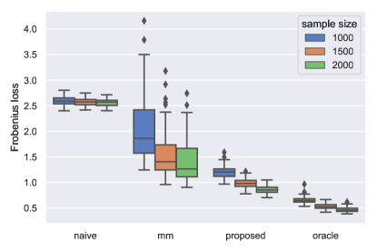
(a) Boxplot for estimating a full rank $\boldsymbol{S}$

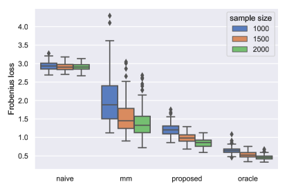
(b) Boxplot for estimating a low rank $\boldsymbol{S}$

Figure 1: Boxplots for Frobenius norm loss over 100 repetitions.

4 Numerical experiments

Regarding parameters for our simulations, we set $T=20$, $p=1.5n$ and $n$ equals successively $1000,1500,2000$. We consider two settings for the noise covariance matrix: $\boldsymbol{S}$ is full-rank and $\boldsymbol{S}$ is low-rank. The complete construction of $\boldsymbol{S}$, $\boldsymbol{B}^{*}$ and $\boldsymbol{X}$, as well as implementation details are given in the supplementary material.

We compare our proposed estimator ${\widehat{\boldsymbol{S}}}$ with relevant estimators including (1) the naive estimate ${\widehat{\boldsymbol{S}}}_{\text{(naive)}}=n^{-1}\boldsymbol{F}^{\top}\boldsymbol{F}$, (2) the method-of-moments estimate ${\widehat{\boldsymbol{S}}}_{\rm{(mm)}}$ defined in Proposition 3.2, and (3) the oracle estimate ${\widehat{\boldsymbol{S}}}_{\rm{(oracle)}}=n^{-1}\boldsymbol{E}^{\top}\boldsymbol{E}$. The performance of each estimator is measured in Frobenius norm: for instance, $\lVert{\widehat{\boldsymbol{S}}}-\boldsymbol{S}\rVert_{\rm{F}}$ is the loss for proposed estimator ${\widehat{\boldsymbol{S}}}$. Figure 1 displays the boxplots of the Frobenius loss from the different methods over 100 repetitions. Figure 1 shows that, besides the oracle estimator, our proposed estimator has the best performance with significantly smaller loss compared to the naive and method-of-moments estimators.

Since the estimation target is a $T\times T$ matrix, we also want to compare different estimators in terms of the bias and standard deviation for each entry of $\boldsymbol{S}$. Figure 2 presents the heatmaps of bias and standard deviation from different estimators for full rank $\boldsymbol{S}$ with $n=1000$. The remaining heatmaps for different $n$ and for estimation of low rank $\boldsymbol{S}$ are available in the supplementary material.

As expected, the oracle estimator has best performance in Figure 1 and smallest bias and variance in Figure 2. The naive estimator has large bias as we see in Figure 2, though it has small standard deviation. The method-of-moments estimator is unbiased but its variance is relatively large, which means its performance is not stable, as was reflected in Figure 1. Our proposed estimator improves on both the naive and method-of-moments estimators because it has much smaller bias than the former, while having smaller standard deviation than the latter.

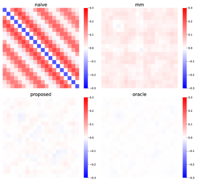
(a) Heatmap of bias for each entry

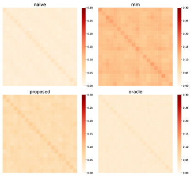
(b) Heatmap of standard deviation for each entry

Figure 2: Heatmaps for estimation of full rank $\boldsymbol{S}$ with $n=1000$ over 100 repetitions.

5 Limitations and future work

One limitation of the proposed estimator ${\widehat{\boldsymbol{S}}}$ is that its construction necessitates the knowledge of $\boldsymbol{\Sigma}$. Let us first mention that the estimator $n^{-1}\lVert(\boldsymbol{I}_{T}-\smash{\widehat{\mathbf{A}}}/n)^{-1}\boldsymbol{F}^{\top}\rVert_{\rm{F}}$ of $\operatorname{Tr}(\boldsymbol{S})+\lVert\boldsymbol{\Sigma}^{1/2}({\widehat{\boldsymbol{B}}}-\boldsymbol{B}^{*})\rVert_{\rm{F}}^{2}$ in Theorem 3.4 does not require knowing $\boldsymbol{\Sigma}$. Thus, this estimator can further be used as a proxy of the error $\lVert\boldsymbol{\Sigma}^{1/2}({\widehat{\boldsymbol{B}}}-\boldsymbol{B}^{*})\rVert_{\rm{F}}^{2}$, say for parameter tuning, without the knowledge of $\boldsymbol{\Sigma}$. The problem of estimating $\boldsymbol{S}$ with known $\boldsymbol{\Sigma}$ was studied in [15] for $T=2$: in this inaccurate covariate model and for $p/n\leq\gamma$, our results yield the convergence rate $n^{-1/2}$ for $\boldsymbol{S}$ which improves upon the rate $n^{-c_{0}}$ for a non-explicit constant $c_{0}>0$ in [15, Theorem 2.1].

In order to use ${\widehat{\boldsymbol{S}}}$ when $\boldsymbol{\Sigma}$ is unknown, one may plug-in an estimator ${\widehat{\boldsymbol{\Sigma}}}$ in Equation 11, resulting in an extra term of order $\lVert{\widehat{\boldsymbol{\Sigma}}}{}^{-1}-\boldsymbol{\Sigma}^{-1}\rVert_{\rm{op}}\lVert\boldsymbol{F}\rVert_{\rm{F}}$ for the Frobenius error. See [17, §4] for related discussions in the $T=1$ (single-task) case. While, under the proportional regime $p/n\to\gamma$, no estimator is consistent for all covariance matrices $\boldsymbol{\Sigma}$ in operator norm, consistent estimators do exist under additional structural assumptions [12, 20, 14]. If available, additional unlabeled samples $(\boldsymbol{x}_{i})_{i\geq n+1}$ can also be used to construct norm-consistent estimator of $\boldsymbol{\Sigma}$.

Future directions include extending estimator ${\widehat{\boldsymbol{S}}}$ to utilize other estimators of the nuisance $\boldsymbol{B}^{*}$ than the multi-task elastic-net (6); for instance (7) or the estimators studied in [36, 30, 11]. In the simpler case where columns of $\boldsymbol{B}^{*}$ are estimated independently on each task, e.g., if the $T$ columns of ${\widehat{\boldsymbol{B}}}$ are Lasso estimators $(\hat{\boldsymbol{\beta}}{}^{(t)})_{t\in[T]}$ each computed from $\boldsymbol{y}{}^{(t)}$, then minor modifications of our proof yield that the estimator (11) with $\smash{\widehat{\mathbf{A}}}=\operatorname{\mathbf{diag}}(\|\hat{\boldsymbol{\beta}}{}^{(1)}\|_{0},...,\|\hat{\boldsymbol{\beta}}{}^{(T)}\|_{0})$ enjoys similar Frobenius norm bounds of order $n^{-1/2}$.

SUPPLEMENT

This supplement is organized as follows:

• In Appendix A we provide details regarding the setting of our simulations, as well as additional experiment results.

• In Appendix B we establish an upper bound for the out-of-sample error, which we could not put in the full paper due to page length limit.

• Appendix C provides the upper bound for $\lVert(\boldsymbol{I}_{T}-\smash{\widehat{\mathbf{A}}}/n)^{-1}\rVert_{\rm{op}}$ mentioned after Theorem 3.3 in the full paper, and Appendices D, E, F contain preliminary theoretical statements, which will be useful for proving our main results in the full paper.

• Appendix G contains proofs of main results in Section 3 of the full paper and Appendix B.

• Appendix H contains proofs of preliminary results in Appendices C to F.

Notation. Here we introduce basic notations that will be used throughout this supplement. We use indexes $i$ and $l$ only to loop or sum over $[n]=\{1,2,\ldots,n\}$, use $j$ and $k$ only to loop or sum over $[p]=\{1,2,\ldots,p\}$, use $t$ and $t^{\prime}$ only to loop or sum over $[T]=\{1,2,\ldots,T\}$, so that $\boldsymbol{e}_{i}$ (and $\boldsymbol{e}_{l}$) refer to the $i$-th (and $l$-th) canonical basis vector in ${\mathbb{R}}^{n}$, $\boldsymbol{e}_{j}$ (and $\boldsymbol{e}_{k}$) refer to the $j$-th (and $k$-th) canonical basis vector in ${\mathbb{R}}^{p}$, $\boldsymbol{e}_{t}$ (and $\boldsymbol{e}_{t^{\prime}}$) refer to the $t$-th (and $t^{\prime}$-th) canonical basis vector in ${\mathbb{R}}^{T}$. For any two real numbers $a$ and $b$, let $a\vee b=\max(a,b)$, and $a\wedge b=\min(a,b)$. Positive constants that depend on $\gamma,\tau^{\prime}$ only are denoted by $C(\gamma,\tau^{\prime})$, and positive constants that depend on $\gamma,c$ only are denoted by $C(\gamma,c)$. The values of these constants may vary from place to place.

Appendix A Experiment details and additional simulation results

A.1 Experimental details

This section provides more experimental detail for Section 4 of the full paper.

We consider two types of noise covariance matrix: (i) $\boldsymbol{S}$ is full-rank with $(t,t^{\prime})$-th entry $\boldsymbol{S}_{t,t^{\prime}}=\frac{\cos(t-t^{\prime})}{1+\sqrt{|t-t^{\prime}|}}$; (ii) $\boldsymbol{S}$ is low-rank with $\boldsymbol{S}=\boldsymbol{u}\boldsymbol{u}^{\top}$, where $\boldsymbol{u}\in{\mathbb{R}}^{T\times 10}$ has i.i.d. entries from ${\cal N}(0,1/T)$.

To build the coefficient matrix $\boldsymbol{B}^{*}$, we first set its sparsity pattern, i.e., we define the support $\mathscr{S}$ of cardinality $|\mathscr{S}|=0.1p$, then we generate an intermediate matrix $\boldsymbol{B}\in{\mathbb{R}}^{p\times T}$. The $j$-th row of $\boldsymbol{B}$ is sampled from ${\cal N}_{T}(\boldsymbol{0},p^{-1}\boldsymbol{I}_{T})$ if $j\in\mathscr{S}$, otherwise we set it to be the zero vector. Finally we let $\boldsymbol{B}^{*}=\boldsymbol{B}[\operatorname{Tr}(\boldsymbol{S})/\operatorname{Tr}(\boldsymbol{B}^{\top}\boldsymbol{\Sigma}\boldsymbol{B})]^{\frac{1}{2}}$, which forces a signal-to-noise ratio of exactly $1$.

The design matrix $\boldsymbol{X}$ is constructed by independently sampling its rows from ${\cal N}_{p}(\boldsymbol{0},\boldsymbol{\Sigma})$ with $\boldsymbol{\Sigma}_{jk}=|j-k|^{0.5}$.

The Python library Scikit-learn [32] is used to calculate ${\widehat{\boldsymbol{B}}}$ in (6). More precisely we invoke MultiTaskElasticNetCV to obtain ${\widehat{\boldsymbol{B}}}$ by 5-fold cross-validation with parameters l1-ratio=[0.5, 0.7, 0.9, 1], n_alpha=100. To compute the interaction matrix $\smash{\widehat{\mathbf{A}}}$ we used the efficient implementation described in [5, Section 5].

The full code needed to reproduce our experiments is part of the supplementary material. A detailed Readme file is located in the corresponding folder.

The simulations results reported in the full paper and this supplementary material were run on a cluster of 50 CPU-cores (each is an Intel Xeon E5-2680 v4 @2.40GHz) equipped with a total of 150 GB of RAM. It takes approximately six hours to obtain all of our simulation results.

A.2 Numerical results of Frobenius norm loss

While Figure 1 in the full paper provides boxplots of Frobenius norm loss for 100 repetitions, we report in following Table 1 the mean and standard deviation of the Frobenius norm loss over 100 repetitions.

Table 1: Comparison of different methods for estimation of $\boldsymbol{S}$

		$n=1000$		$n=1500$		$n=2000$
$\boldsymbol{S}$	method	mean	sd	mean	sd	mean	sd
full rank	naive	2.593	0.090	2.572	0.076	2.562	0.070
	mm	2.030	0.616	1.554	0.421	1.413	0.405
	proposed	1.207	0.119	0.984	0.084	0.858	0.072
	oracle	0.652	0.061	0.534	0.052	0.469	0.045
low rank	naive	2.942	0.119	2.912	0.102	2.908	0.094
	mm	2.027	0.686	1.561	0.435	1.423	0.414
	proposed	1.216	0.172	0.989	0.125	0.854	0.118
	oracle	0.654	0.096	0.531	0.081	0.464	0.065

The numerical results in Table 1 are consistent with the boxplots in Figure 1. It is clear from Table 1 that our proposed estimator has significantly smaller loss than the naive estimator and method-of-moments estimator. These comparisons again show the superior performance of our proposed estimator.

A.3 Additional heatmaps for estimating full rank $\boldsymbol{S}$

When estimating the full rank $\boldsymbol{S}$ with $(t,t^{\prime})$-th entry $\boldsymbol{S}_{t,t^{\prime}}=\frac{\cos(t-t^{\prime})}{1+\sqrt{|t-t^{\prime}|}}$, the heatmaps for different estimators from $n=1500$ and $n=2000$ are presented in Figures 3 and 4, respectively. The comparison patterns in Figures 3 and 4 are similar to the case $n=1000$ in Figure 2 of the full paper; our proposed estimator outperforms the naive estimator and method-of-moments estimator.

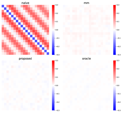
(a) Heatmap of bias for each entry

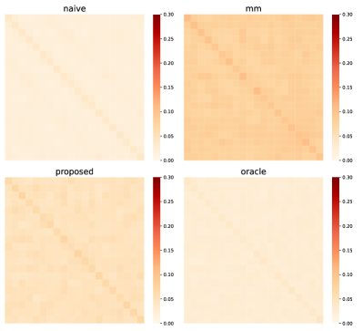
(b) Heatmap of standard deviation in each entry

Figure 3: Heatmaps for estimation of full rank $\boldsymbol{S}$ with $n=1500$ over 100 repetitions.

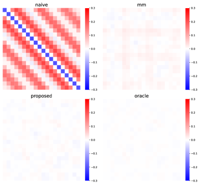
(a) Heatmap of bias for each entry

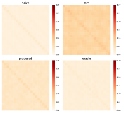
(b) Heatmap of standard deviation in each entry

Figure 4: Heatmaps for estimation of full rank $\boldsymbol{S}$ with $n=2000$ over 100 repetitions.

A.4 Heatmaps for estimating low rank $\boldsymbol{S}$

When estimating the low rank with $\boldsymbol{S}=\boldsymbol{u}\boldsymbol{u}^{\top}$, and $\boldsymbol{u}\in{\mathbb{R}}^{T\times 10}$ with entries are i.i.d. from ${\cal N}(0,1/T)$. We present the heatmaps for different estimators with $n=1000,1500,2000$ in Figures 5, 6 and 7 below. All of these figures convince us that besides the oracle estimator, the proposed estimator has the best performance.

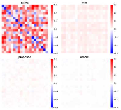
(a) Heatmap of bias for each entry

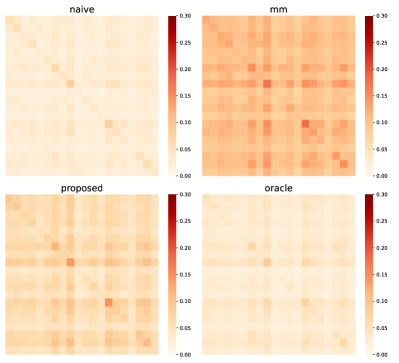
(b) Heatmap of standard deviation in each entry

Figure 5: Heatmaps for estimation of low rank $\boldsymbol{S}$ with $n=1000$ over 100 repetitions.

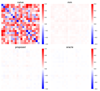
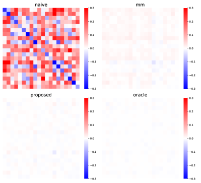
(a) Heatmap of bias for each entry

(b) Heatmap of standard deviation in each entry

Figure 6: Heatmaps for estimation of low rank $\boldsymbol{S}$ with $n=1500$ over 100 repetitions.

(a) Heatmap of bias for each entry

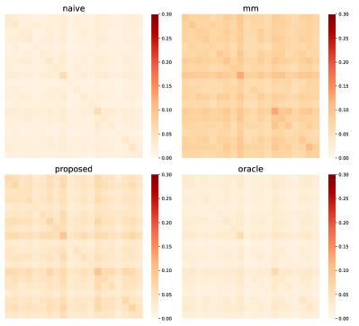
(b) Heatmap of standard deviation in each entry

Figure 7: Heatmaps for estimation of low rank $\boldsymbol{S}$ with $n=2000$ over 100 repetitions.

Appendix B Out-of-sample error estimation

In this appendix, we present a by-product of our techniques for estimating the noise covariance. Suppose we wish to evaluate the performance of a regression method on a new data, we define the out-of-sample error for the multi-task linear model (1) as

$${\mathbb{E}}\big{[}({\widehat{\boldsymbol{B}}}-\boldsymbol{B}^{*})^{\top}\boldsymbol{x}_{\text{new}}\boldsymbol{x}_{\text{new}}^{\top}({\widehat{\boldsymbol{B}}}-\boldsymbol{B}^{*})|(\boldsymbol{X},\boldsymbol{Y})\big{]}=\boldsymbol{H}^{\top}\boldsymbol{H},$$

where $\boldsymbol{x}_{\text{new}}$ is independent of the data $(\boldsymbol{X};\boldsymbol{Y})$ with the same distribution as any row of $\boldsymbol{X}$.

The following theorem on estimation of out-of-sample error is an by-product of our technique for constructing ${\widehat{\boldsymbol{S}}}$.

Theorem B.1 (Out-of-sample error).

Under the same conditions of Theorem 3.3, with $\boldsymbol{Z}=\boldsymbol{X}\boldsymbol{\Sigma}^{-\frac{1}{2}}$, we have

$$\lVert(\boldsymbol{I}_{T}-\smash{\widehat{\mathbf{A}}}/n)\boldsymbol{H}^{\top}\boldsymbol{H}(\boldsymbol{I}_{T}-\smash{\widehat{\mathbf{A}}}/n)-\frac{1}{n^{2}}\big{(}\boldsymbol{F}^{\top}\boldsymbol{Z}\boldsymbol{Z}^{\top}\boldsymbol{F}+\smash{\widehat{\mathbf{A}}}\boldsymbol{F}^{\top}\boldsymbol{F}+\boldsymbol{F}^{\top}\boldsymbol{F}\smash{\widehat{\mathbf{A}}}-p\boldsymbol{F}^{\top}\boldsymbol{F}\big{)}\rVert_{\rm{F}}$$

$$\leq \Theta_{3}n^{-\frac{1}{2}}(\lVert\boldsymbol{H}\rVert_{\rm{F}}^{2}+\left\lVert\boldsymbol{F}\right\rVert_{\rm{F}}^{2}/n)$$

for some non-negative random variable $\Theta_{3}$ of constant order, in the sense that ${\mathbb{E}}[\Theta_{3}]\leq C(\gamma,\tau^{\prime})$ under Assumption 4(i), and with ${{\mathbb{E}}[I(\Omega)\Theta_{3}]}\leq C(\gamma,c)$ under Assumption 4(ii), where $I(\Omega)$ is the indicator function of an event $\Omega$ with ${\mathbb{P}}(\Omega)\to 1$.

Theorem B.1 generalizes the result in [4] to multi-task setting. While the out-of-sample error $\boldsymbol{H}^{\top}\boldsymbol{H}$ is unknown, the quantities $\boldsymbol{Z}$, $\boldsymbol{F}$, $\smash{\widehat{\mathbf{A}}}$ are observable. Since typically the quantity $(\lVert\boldsymbol{H}\rVert_{\rm{F}}^{2}+\left\lVert\boldsymbol{F}\right\rVert_{\rm{F}}^{2}/n)$ is of a constant order, Theorem B.1 suggests the following estimate of $\boldsymbol{H}^{\top}\boldsymbol{H}$:

$$\frac{1}{n^{2}}(\boldsymbol{I}_{T}-\smash{\widehat{\mathbf{A}}}/n)^{-1}\big{(}\boldsymbol{F}^{\top}\boldsymbol{Z}\boldsymbol{Z}^{\top}\boldsymbol{F}+\smash{\widehat{\mathbf{A}}}\boldsymbol{F}^{\top}\boldsymbol{F}+\boldsymbol{F}^{\top}\boldsymbol{F}\smash{\widehat{\mathbf{A}}}-p\boldsymbol{F}^{\top}\boldsymbol{F}\big{)}(\boldsymbol{I}_{T}-\smash{\widehat{\mathbf{A}}}/n)^{-1},$$

which can further be used for parameter tuning in multi-task linear model.

We present the proof of Theorem B.1 in Section G.8

Appendix C Useful operator norm bounds

Let us first introduce two events besides the event $U_{1}=\big{\{}\lVert{\widehat{\boldsymbol{B}}}\rVert_{0}\leq n(1-c)/2\big{\}}$ in Assumption 4(ii), we define events $U_{2}$ and $U_{3}$ as below,

$$U_{2} =\big{\{}\inf_{\boldsymbol{b}\in{\mathbb{R}}^{p}:\|\boldsymbol{b}\|_{0}\leq(1-c)n}\|\boldsymbol{X}\boldsymbol{b}\|^{2}/(n\|\boldsymbol{\Sigma}^{\frac{1}{2}}\boldsymbol{b}\|^{2})>\eta\big{\}},$$

$$U_{3} =\big{\{}\lVert\boldsymbol{X}\boldsymbol{\Sigma}^{-\frac{1}{2}}\rVert_{\rm{op}}<2\sqrt{n}+\sqrt{p}\big{\}}.$$

Under Assumptions 2 and 3, [7, Lemma B.1] guarantees ${\mathbb{P}}(U_{2})\geq 1-C(\gamma,c)e^{-C(\gamma,c)n}$ for some constant $\eta$ that only depends on constants $\gamma,c$. Under Assumption 2, [16, Theorem II.13] guarantees ${\mathbb{P}}(U_{3})>1-e^{-n/2}$ and there exists a random variable $z\sim{\cal N}(0,1)$ s.t. $\lVert\boldsymbol{X}\boldsymbol{\Sigma}^{-\frac{1}{2}}\rVert_{\rm{op}}\leq\sqrt{n}+\sqrt{p}+z$ almost surely. Therefore, under Assumptions 2 and 3, we have

$${\mathbb{E}}[\lVert n^{-\frac{1}{2}}\boldsymbol{X}\boldsymbol{\Sigma}^{-\frac{1}{2}}\rVert_{\rm{op}}^{2}]\leq(1+\sqrt{p/n})^{2}+n^{-1}\leq C(\gamma).$$ (23)

Furthermore, under Assumptions 3, LABEL:, 2, LABEL: and 4(ii), ${\mathbb{P}}(U_{1}\cap U_{2}\cap U_{3})\to 1$ by a union bound, and for large enough $n$,

$${\mathbb{P}}\big{\{}(U_{1}\cap U_{2}\cap U_{3})^{c}\big{\}}< 1/T+C(\gamma,c)e^{-n/C(\gamma,c)}$$

$$= \frac{1}{T}(1+TC(\gamma,c)e^{-n/C(\gamma,c)})$$

$$< \frac{1}{T}(1+C(\gamma,c)e^{\sqrt{n}-n/C(\gamma,c)})$$

$$< \frac{1}{T}C(\gamma,c).$$ (24)

Now we provide the operator norm bounds for $\boldsymbol{I}_{T}-\smash{\widehat{\mathbf{A}}}/n$ and $(\boldsymbol{I}_{T}-\smash{\widehat{\mathbf{A}}}/n)^{-1}$.

Lemma C.1.

Suppose that Assumption 2 holds. If $\tau>0$ in (6) with $\tau^{\prime}=\tau/\lVert\boldsymbol{\Sigma}\rVert_{\rm{op}}$, then

1. $\lVert\boldsymbol{I}_{T}-\smash{\widehat{\mathbf{A}}}/n\rVert_{\rm{op}}\leq 1$.

2. In the event $U_{3}$, we have $\lVert(\boldsymbol{I}_{T}-\smash{\widehat{\mathbf{A}}}/n)^{-1}\rVert_{\rm{op}}\leq 1+(\tau^{\prime})^{-1}(2+\sqrt{p/n})^{2}$. Furthermore, ${\mathbb{E}}[\lVert(\boldsymbol{I}_{T}-\smash{\widehat{\mathbf{A}}}/n)^{-1}\rVert_{\rm{op}}]\leq 1+(\tau^{\prime})^{-1}[(1+\sqrt{p/n})^{2}+n^{-1}].$

Lemma C.2.

Suppose that Assumption 2 holds. If $\tau=0$ in (6), then

1. In the event $U_{1}$, we have $\lVert\boldsymbol{I}_{T}-\smash{\widehat{\mathbf{A}}}/n\rVert_{\rm{op}}\leq 1$.

2. In the event $U_{1}$, $\lVert(\boldsymbol{I}_{T}-\smash{\widehat{\mathbf{A}}}/n)^{-1}\rVert_{\rm{op}}\leq C(c)$. Hence, ${\mathbb{E}}[I(U_{1})\lVert(\boldsymbol{I}_{T}-\smash{\widehat{\mathbf{A}}}/n)^{-1}\rVert_{\rm{op}}]\leq C(c).$

Lemma C.3.

With $\boldsymbol{N}=(\boldsymbol{I}_{T}\otimes\boldsymbol{X})\boldsymbol{M}^{\dagger}(\boldsymbol{I}_{T}\otimes\boldsymbol{X}^{\top})$, we have $\lVert\boldsymbol{N}\rVert_{\rm{op}}\leq 1$.

Appendix D Lipschitz and differential properties for a given, fixed noise matrix $\boldsymbol{E}$

We need to study Lipschitz and differential properties of certain mappings when the noise matrix $\boldsymbol{E}$ is fixed. Let $g:{\mathbb{R}}^{p\times T}\to{\mathbb{R}}$ defined by $g(\boldsymbol{B})=\tau\lVert\boldsymbol{B}\rVert_{\rm{F}}^{2}/2+\lambda\lVert\boldsymbol{B}\rVert_{2,1}$ be the penalty in (6). For a fixed value of $\boldsymbol{E}$, define the mappings

$$\boldsymbol{Z} \longmapsto\boldsymbol{H}(\boldsymbol{Z})=\mathop{\rm arg\,min}_{\bar{\boldsymbol{H}}\in{\mathbb{R}}^{p\times T}}\frac{1}{2n}\lVert\boldsymbol{E}-\boldsymbol{Z}\bar{\boldsymbol{H}}\rVert_{\rm{F}}^{2}+g(\boldsymbol{\Sigma}^{-1/2}\bar{\boldsymbol{H}}) ({\mathbb{R}}^{n\times p}\to{\mathbb{R}}^{p\times T})$$ (25)

$$\boldsymbol{Z} \longmapsto\boldsymbol{F}(\boldsymbol{Z})=\boldsymbol{E}-\boldsymbol{Z}\boldsymbol{H}(\boldsymbol{Z}) ({\mathbb{R}}^{n\times p}\to{\mathbb{R}}^{n\times T})$$ (26)

$$\boldsymbol{Z} \longmapsto D(\boldsymbol{Z})=(\lVert\boldsymbol{H}(\boldsymbol{Z})\rVert_{\rm{F}}^{2}+\lVert\boldsymbol{F}(\boldsymbol{Z})\rVert_{\rm{F}}^{2}/n)^{1/2} ({\mathbb{R}}^{n\times p}\to{\mathbb{R}}).$$ (27)

Next, define the random variable $\boldsymbol{Z}=\boldsymbol{X}\boldsymbol{\Sigma}^{-\frac{1}{2}}\in{\mathbb{R}}^{n\times p}$, and let us use the convention that if arguments of $\boldsymbol{H},\boldsymbol{F}$ or $D$ are omitted then these mappings are implicitly taken at the realized value of the random variable $\boldsymbol{Z}=\boldsymbol{X}\boldsymbol{\Sigma}^{-\frac{1}{2}}\in{\mathbb{R}}^{n\times p}$ where $\boldsymbol{X}$ is the observed design matrix. With this convention and by definition of the above mappings, we then have $\boldsymbol{H}=\boldsymbol{H}(\boldsymbol{Z})=\boldsymbol{\Sigma}^{1/2}({\widehat{\boldsymbol{B}}}-\boldsymbol{B}^{*})$ as well as $\boldsymbol{F}=\boldsymbol{F}(\boldsymbol{Z})=\boldsymbol{Y}-\boldsymbol{X}{\widehat{\boldsymbol{B}}}$ and $D=[\lVert\boldsymbol{H}\rVert_{\rm{F}}^{2}+\lVert\boldsymbol{F}\rVert_{\rm{F}}^{2}/n]^{1/2}$ so that the notation is consistent with the rest of the paper (in particular, with (9)).

Finally, denote the $(i,j)$-th entry of $\boldsymbol{Z}$ by $z_{ij}$ throughout this appendix, and the corresponding partial derivatives of the above mappings by $\frac{\partial}{\partial z_{ij}}$.

D.1 Lipschitz properties

Lemma D.1.

For multi-task elastic-net (i.e., $\tau>0$ in (6)), the mapping $\boldsymbol{Z}\mapsto D^{-1}\boldsymbol{F}/\sqrt{n}$ is $n^{-\frac{1}{2}}L$-Lipschitz with $L=8\max(1,(2\tau^{\prime})^{-1})$, where $\tau^{\prime}=\tau/\lVert\boldsymbol{\Sigma}\rVert_{\rm{op}}$.

Lemma D.2.

For multi-task group Lasso (i.e., $\tau=0$ in (6)). we have

• In $U_{1}\cap U_{2}$, the map $\boldsymbol{Z}\mapsto D^{-1}\boldsymbol{F}/\sqrt{n}$ is $n^{-\frac{1}{2}}L$-Lipschitz with $L=8\max(1,(2\eta)^{-1})$.

• In $U_{1}\cap U_{2}\cap U_{3}$, the map $\boldsymbol{Z}\mapsto D^{-1}\boldsymbol{Z}^{\top}\boldsymbol{F}/n$ is $n^{-1/2}(1+(2+\sqrt{p/n})L)$-Lipschitz, where $L=8\max(1,(2\eta)^{-1})$ as in (1).

Corollary D.3.

Suppose that Assumption 4 holds, then

• Under Assumption 4(i) that $\tau>0$ and $\tau^{\prime}=\tau/\lVert\boldsymbol{\Sigma}\rVert_{\rm{op}}$, we have

  $$\sum_{ij}\Big{(}\frac{\partial D}{\partial z_{ij}}\Big{)}^{2}\leq n^{-1}D^{2}[4\max(1,(2\tau^{\prime})^{-1})]^{2}.$$

  This implies that $nD^{-2}\sum_{ij}(\frac{\partial D}{\partial z_{ij}})^{2}\leq C(\tau^{\prime}).$

• Under Assumption 4(ii) that $\tau=0$ and ${\mathbb{P}}(U_{1})\to 1$, in the event $U_{1}\cap U_{2}$, we have

  $$\sum_{ij}\Big{(}\frac{\partial D}{\partial z_{ij}}\Big{)}^{2}\leq n^{-1}D^{2}[4\max(1,(2\eta)^{-1})]^{2}.$$

  This implies that $nD^{-2}\sum_{ij}(\frac{\partial D}{\partial z_{ij}})^{2}\leq C(\eta)=C(\gamma,c)$ since $\eta$ is a constant that only depends on $\gamma,c$.

D.2 Derivative formulae

Note that with a fixed noise $\boldsymbol{E}$, Lemmas D.1 and D.2 guarantee that the map $\boldsymbol{Z}\mapsto\boldsymbol{F}$ is Lipschitz, hence the derivative exists almost everywhere by Rademacher’s theorem. We present the formula for derivative of this map in Lemma D.4.

Lemma D.4.

Recall $\boldsymbol{F}=\boldsymbol{Y}-\boldsymbol{X}{\widehat{\boldsymbol{B}}}$ with ${\widehat{\boldsymbol{B}}}$ defined in (6). Under Assumption 4(i) $\tau>0$, or under Assumption 4(ii) $\tau=0$ and in the event $U_{1}\cap U_{2}$, for each $i,l\in[n],j\in[p],t\in[T]$, the following derivative exists almost everywhere and has the expression

$$\frac{\partial F_{lt}}{\partial z_{ij}}=D_{ij}^{lt}+\Delta_{ij}^{lt},$$

where $D_{ij}^{lt}=-(\boldsymbol{e}_{j}^{\top}\boldsymbol{H}\otimes\boldsymbol{e}_{i}^{\top})(\boldsymbol{I}_{nT}-\boldsymbol{N})(\boldsymbol{e}_{t}\otimes\boldsymbol{e}_{l}),$ and $\Delta_{ij}^{lt}=-(\boldsymbol{e}_{t}^{\top}\otimes\boldsymbol{e}_{l}^{\top})(\boldsymbol{I}_{T}\otimes\boldsymbol{X})\boldsymbol{M}^{\dagger}(\boldsymbol{I}_{T}\otimes\boldsymbol{\Sigma}^{\frac{1}{2}})\bigl{(}\boldsymbol{F}^{\top}\otimes\boldsymbol{I}_{p}\bigr{)}(\boldsymbol{e}_{i}\otimes\boldsymbol{e}_{j}).$ Furthermore, a straightforward calculation yields

$$\sum_{i=1}^{n}D_{ij}^{it}=-\boldsymbol{e}_{j}^{\top}\boldsymbol{H}(n\boldsymbol{I}_{T}-\smash{\widehat{\mathbf{A}}})\boldsymbol{e}_{t}.$$

Lemma D.5.

Suppose that Assumption 4 holds.

• Under Assumption 4(i) that $\tau>0$ and $\tau^{\prime}=\tau/\lVert\boldsymbol{\Sigma}\rVert_{\rm{op}}$, we have

  $$\frac{1}{n}\sum_{ij}\left\lVert\frac{\partial(\boldsymbol{F}/D)}{\partial z_{ij}}\right\rVert^{2}_{\rm F}\leq\underbrace{4\max(1,(\tau^{\prime})^{-1}(T\wedge\frac{p}{n}))+2n^{-1}[4\max(1,(2\tau^{\prime})^{-1})]^{2}}_{f(\tau^{\prime},T,n,p)}.$$

• Under Assumption 4(ii) that $\tau=0$ and ${\mathbb{P}}(U_{1})\to 1$, in the event $U_{1}\cap U_{2}$, we have

  $$\frac{1}{n}\sum_{ij}\left\lVert\frac{\partial(\boldsymbol{F}/D)}{\partial z_{ij}}\right\rVert^{2}_{\rm F}\leq\underbrace{4\max(1,(\eta)^{-1}(T\wedge\frac{p}{n}))+2n^{-1}[4\max(1,(2\eta)^{-1})]^{2}}_{f(\eta,T,n,p)}.$$

Furthermore, the right-hand side in (1) can be bounded from above by $C(\tau^{\prime})(T\wedge\frac{p}{n})$, and the right-hand side in (2) can be bounded from above by $C(\gamma,c)$ in the regime $p/n\leq\gamma$.

Appendix E Lipschitz and differential properties for a given, fixed design matrix

We also need to study Lipschitz and derivative properties of functions of the noise $\boldsymbol{E}$ when the design $\boldsymbol{X}$ is fixed. Formally, for a given and fixed design matrix $\boldsymbol{X}$, define the function $\boldsymbol{E}\mapsto\boldsymbol{F}(\boldsymbol{E})$ by the value $\boldsymbol{Y}-\boldsymbol{X}{\widehat{\boldsymbol{B}}}$ of the residual matrix when the observed data $(\boldsymbol{X},\boldsymbol{Y})$ is $(\boldsymbol{X},\boldsymbol{X}\boldsymbol{B}^{*}+\boldsymbol{E})$ and with ${\widehat{\boldsymbol{B}}}$ the estimator (6). Note that this map is 1-Lipschitz by [6, proposition 3]. Rademacher’s theorem thus guarantees this map is differentiable almost everywhere. We denote its partial derivative by $\frac{\partial}{\partial E_{it}}$ for each entry $(E_{it})_{i\in[n],t\in[T]}$ of the noise matrix $\boldsymbol{E}$. We present its derivative formula in Lemma E.1 below.

Lemma E.1.

For each $i,l\in[n],t,t^{\prime}\in[T]$, the following derivative exists almost everywhere and has the expression

$$\frac{\partial F_{lt}}{\partial E_{it^{\prime}}}=\boldsymbol{e}_{l}^{\top}\boldsymbol{e}_{i}\boldsymbol{e}_{t}^{\top}\boldsymbol{e}_{t^{\prime}}-\boldsymbol{e}_{l}^{\top}(\boldsymbol{e}_{t}^{\top}\otimes\boldsymbol{X})\boldsymbol{M}^{\dagger}(\boldsymbol{e}_{t^{\prime}}\otimes\boldsymbol{X}^{\top})\boldsymbol{e}_{i}.$$

As a consequence, we further have

$$\sum_{i=1}^{n}\frac{\partial F_{it}}{\partial E_{it^{\prime}}}=\boldsymbol{e}_{t}^{\top}(n\boldsymbol{I}_{T}-\smash{\widehat{\mathbf{A}}})\boldsymbol{e}_{t^{\prime}},\quad\sum_{i=1}^{n}\frac{\partial\boldsymbol{e}_{i}^{\top}\boldsymbol{Z}\boldsymbol{H}\boldsymbol{e}_{t}}{\partial E_{it^{\prime}}}=\boldsymbol{e}_{t}^{\top}\smash{\widehat{\mathbf{A}}}\boldsymbol{e}_{t^{\prime}}.$$

Appendix F Probabilistic tools

We first list some useful variants of Stein’s formulae and Gaussian-Poincaré inequalities. Let $f^{\prime}$ denote the derivative of a differentiable univariate function. For a differentiable vector-valued function $\boldsymbol{f}(\boldsymbol{z}):{\mathbb{R}}^{n}\to{\mathbb{R}}^{n}$, denote its Jacobian (derivative) and divergence respectively by $\nabla\boldsymbol{f}(\boldsymbol{z})$ and $\operatorname{div}\boldsymbol{f}(\boldsymbol{z})$, i.e., $[\nabla\boldsymbol{f}(\boldsymbol{z})]_{i,l}=\frac{\partial f_{i}(\boldsymbol{z})}{\partial z_{l}}$ for $i,l\in[n]$, and $\operatorname{div}\boldsymbol{f}(\boldsymbol{z})=\operatorname{Tr}(\nabla\boldsymbol{f}(\boldsymbol{z}))$.

Lemma F.1 (Second-order Stein’s formula [8]).

The following identities hold provided the involved derivatives exist a.e. and the expectations are finite.

1. $z\sim{\cal N}(0,1)$, $f:{\mathbb{R}}\to{\mathbb{R}}$, then

   $${\mathbb{E}}[(zf(z)-f^{\prime}(z))^{2}]={\mathbb{E}}[f(z)^{2}]+{\mathbb{E}}[(f^{\prime}(z))^{2}].$$

2. $\boldsymbol{z}\sim{\cal N}_{n}(\boldsymbol{0},\boldsymbol{I}_{n})$, $f:{\mathbb{R}}^{n}\to{\mathbb{R}}^{n}$, then

   $${\mathbb{E}}[(\boldsymbol{z}^{\top}\boldsymbol{f}(\boldsymbol{z})-\operatorname{div}\boldsymbol{f}(\boldsymbol{z}))^{2}]={\mathbb{E}}\big{[}\lVert\boldsymbol{f}(\boldsymbol{z})\rVert^{2}+\operatorname{Tr}[(\nabla\boldsymbol{f}(\boldsymbol{z}))^{2}]\big{]}\leq{\mathbb{E}}\big{[}\lVert\boldsymbol{f}(\boldsymbol{z})\rVert^{2}+\lVert\nabla\boldsymbol{f}(\boldsymbol{z})\rVert_{\rm{F}}^{2}\big{]},$$

   where the inequality uses Cauchy-Schwarz inequality.

3. More generally, for $\boldsymbol{z}\sim{\cal N}_{n}(\boldsymbol{0},\boldsymbol{\Sigma})$, $\boldsymbol{f}:{\mathbb{R}}^{n}\to{\mathbb{R}}^{n}$, then

   $${\mathbb{E}}[(\boldsymbol{z}^{\top}\boldsymbol{f}(\boldsymbol{z})-\operatorname{Tr}(\boldsymbol{\Sigma}\nabla\boldsymbol{f}(\boldsymbol{z}))^{2}] ={\mathbb{E}}\big{[}\lVert\boldsymbol{\Sigma}^{\frac{1}{2}}\boldsymbol{f}(\boldsymbol{z})\rVert^{2}+\operatorname{Tr}[(\boldsymbol{\Sigma}\nabla\boldsymbol{f}(\boldsymbol{z}))^{2}]\big{]}$$

   $$\leq{\mathbb{E}}\big{[}\lVert\boldsymbol{\Sigma}^{\frac{1}{2}}\boldsymbol{f}(\boldsymbol{z})\rVert^{2}+\lVert(\boldsymbol{\Sigma}\nabla\boldsymbol{f}(\boldsymbol{z})\rVert_{\rm{F}}^{2}]\big{]},$$

   where the inequality uses Cauchy-Schwarz inequality.

Lemma F.2 (Gaussian-Poincaré inequality [13]).

The following inequalities hold provided the right-hand side derivatives exist a.e. and the expectations are finite.

1. $z\sim{\cal N}(0,1)$, $f:{\mathbb{R}}\to{\mathbb{R}}$, then

   $$\text{Var}[f(z)]\leq{\mathbb{E}}[(f^{\prime}(z))^{2}].$$

2. $\boldsymbol{z}\sim{\cal N}_{n}(\boldsymbol{0},\boldsymbol{I}_{n})$, $f:{\mathbb{R}}^{n}\to{\mathbb{R}}$, then

   $$\text{Var}[f(\boldsymbol{z})]\leq{\mathbb{E}}[\lVert\nabla f(\boldsymbol{z})\rVert^{2}].$$

3. $\boldsymbol{z}\sim{\cal N}_{n}(\boldsymbol{0},\boldsymbol{I}_{n})$, $\boldsymbol{f}:{\mathbb{R}}^{n}\to{\mathbb{R}}^{m}$, then

   $${\mathbb{E}}[\lVert\boldsymbol{f}(\boldsymbol{z})-{\mathbb{E}}[\boldsymbol{f}(\boldsymbol{z})]\rVert^{2}]\leq{\mathbb{E}}[\lVert\nabla\boldsymbol{f}(\boldsymbol{z})\rVert_{\rm{F}}^{2}].$$

4. More generally, for $\boldsymbol{z}\sim{\cal N}_{n}(\boldsymbol{0},\boldsymbol{\Sigma})$, $\boldsymbol{f}:{\mathbb{R}}^{n}\to{\mathbb{R}}^{m}$, then

   $${\mathbb{E}}[\lVert\boldsymbol{f}(\boldsymbol{z})-{\mathbb{E}}[\boldsymbol{f}(\boldsymbol{z})]\rVert^{2}]\leq{\mathbb{E}}[\lVert\boldsymbol{\Sigma}^{\frac{1}{2}}\nabla\boldsymbol{f}(\boldsymbol{z})\rVert_{\rm{F}}^{2}].$$

Now we present a few important lemmas, whose proofs are based on Lemma F.1 and Lemma F.2.

Lemma F.3.

Assume that Assumption 1 holds. For fixed $\boldsymbol{X}$, we have

$${\mathbb{E}}\Bigl{[}\lVert\boldsymbol{E}^{\top}\boldsymbol{F}/{\tilde{D}}-\boldsymbol{S}(n\boldsymbol{I}_{T}-\smash{\widehat{\mathbf{A}}})/{\tilde{D}}\rVert_{\rm{F}}^{2}\Bigr{]}\leq 4\operatorname{Tr}(\boldsymbol{S}),$$

where ${\tilde{D}}=\big{(}\left\lVert\boldsymbol{F}\right\rVert_{\rm{F}}^{2}+n\operatorname{Tr}(\boldsymbol{S})\big{)}^{\frac{1}{2}}$.

Lemma F.4.

Let $\boldsymbol{U},\boldsymbol{V}:{\mathbb{R}}^{n\times p}\to{\mathbb{R}}^{n\times T}$ be two locally Lipschitz functions of $\boldsymbol{Z}$ with i.i.d. ${\cal N}(0,1)$ entries, then

$${\mathbb{E}}\Big{[}\Big{\lVert}\boldsymbol{U}^{\top}\boldsymbol{Z}\boldsymbol{V}-\sum_{j=1}^{p}\sum_{i=1}^{n}\frac{\partial}{\partial z_{ij}}\Bigl{(}\boldsymbol{U}^{\top}\boldsymbol{e}_{i}\boldsymbol{e}_{j}^{\top}\boldsymbol{V}\Bigr{)}\Big{\rVert}_{\rm F}^{2}\Big{]}$$

$$\leq~{} {\mathbb{E}}\left\lVert\boldsymbol{U}\right\rVert_{\rm{F}}^{2}\left\lVert\boldsymbol{V}\right\rVert_{\rm{F}}^{2}+{\mathbb{E}}\sum_{ij}\Big{[}2\left\lVert\boldsymbol{V}\right\rVert_{\rm{F}}^{2}\left\lVert\frac{\partial\boldsymbol{U}}{\partial z_{ij}}\right\rVert_{\rm{F}}^{2}+2\left\lVert\boldsymbol{U}\right\rVert_{\rm{F}}^{2}\left\lVert\frac{\partial\boldsymbol{V}}{\partial z_{ij}}\right\rVert_{\rm{F}}^{2}\Big{]}.$$

Corollary F.5.

Assume the same setting as Lemma F.4. If on some open set $\Omega\subset{\mathbb{R}}^{n\times p}$ with ${\mathbb{P}}(\Omega^{c})\leq C/T$ for some constant $C$, we have (i) $\boldsymbol{U}$ is $n^{-1/2}L_{1}$ -Lipschitz and $\lVert\boldsymbol{U}\rVert_{\rm{F}}\leq 1$, (ii) $\boldsymbol{V}$ is $n^{-1/2}L_{2}$ -Lipschitz and $\lVert\boldsymbol{V}\rVert_{\rm{F}}\leq K$. Then

$${\mathbb{E}}\Big{[}I(\Omega)\Big{\|}\boldsymbol{U}^{\top}\boldsymbol{Z}\boldsymbol{V}-\sum_{j=1}^{p}\sum_{i=1}^{n}\frac{\partial}{\partial z_{ij}}\Bigl{(}\boldsymbol{U}^{\top}\boldsymbol{e}_{i}\boldsymbol{e}_{j}^{\top}\boldsymbol{V}\Bigr{)}\Big{\|}_{\rm F}^{2}\Big{]}$$

$$\leq~{} K^{2}+2C(K^{2}L_{1}^{2}+L_{2}^{2})+2{\mathbb{E}}\Big{[}I(\Omega)\sum_{ij}\Big{(}K^{2}\left\lVert\frac{\partial\boldsymbol{U}}{\partial z_{ij}}\right\rVert_{\rm{F}}^{2}+\left\lVert\frac{\partial\boldsymbol{V}}{\partial z_{ij}}\right\rVert_{\rm{F}}^{2}\Big{)}\Big{]}.$$

Lemma F.6.

Let $\boldsymbol{U},\boldsymbol{V}:{\mathbb{R}}^{n\times p}\to{\mathbb{R}}^{n\times T}$ be two locally Lipschitz functions of $\boldsymbol{Z}$ with i.i.d. ${\cal N}(0,1)$ entries. Assume also that $\lVert\boldsymbol{U}\rVert_{\rm{F}}\vee\lVert\boldsymbol{V}\rVert_{\rm{F}}\leq 1$ almost surely. Then

$${\mathbb{E}}\Bigl{[}\Big{\lVert}p\boldsymbol{U}^{\top}\boldsymbol{V}-\sum_{j=1}^{p}\Bigl{(}\sum_{i=1}^{n}\partial_{ij}\boldsymbol{U}^{\top}\boldsymbol{e}_{i}-\boldsymbol{U}^{\top}\boldsymbol{Z}\boldsymbol{e}_{j}\Bigr{)}\Bigl{(}\sum_{i=1}^{n}\partial_{ij}\boldsymbol{e}_{i}^{T}\boldsymbol{V}-\boldsymbol{e}_{j}^{T}\boldsymbol{Z}^{T}\boldsymbol{V}\Bigr{)}\Big{\rVert}_{\rm{F}}\Bigr{]}$$

$$\leq~{} 2\|\boldsymbol{U}\|_{\partial}\|\boldsymbol{V}\|_{\partial}+\sqrt{p}\bigl{(}\sqrt{2}+(3+\sqrt{2})(\|\boldsymbol{U}\|_{\partial}+\|\boldsymbol{V}\|_{\partial})\bigr{)},$$

where $\partial_{ij}\boldsymbol{U}\stackrel{{\scriptstyle\text{\tiny def}}}{{=}}\partial\boldsymbol{U}/\partial z_{ij}$, and $\|\boldsymbol{U}\|_{\partial}\stackrel{{\scriptstyle\text{\tiny def}}}{{=}}{\mathbb{E}}[\sum_{i=1}^{n}\sum_{j=1}^{p}\lVert\partial_{ij}\boldsymbol{U}\rVert_{\rm{F}}^{2}]^{\frac{1}{2}}$.

Proposition F.7.

Suppose that Assumption 1 holds.
Let $\boldsymbol{Q}_{1}=\frac{\frac{1}{n}\big{(}\boldsymbol{F}^{\top}\boldsymbol{F}+\boldsymbol{H}^{\top}\boldsymbol{Z}^{\top}\boldsymbol{F}-\boldsymbol{S}(n\boldsymbol{I}_{T}-\smash{\widehat{\mathbf{A}}})\big{)}}{\lVert\boldsymbol{S}^{\frac{1}{2}}\rVert_{\rm{F}}(\left\lVert\boldsymbol{F}\right\rVert_{\rm{F}}^{2}/n+\operatorname{Tr}(\boldsymbol{S}))^{\frac{1}{2}}n^{-\frac{1}{2}}}$, then ${\mathbb{E}}[\left\lVert\boldsymbol{Q}_{1}\right\rVert_{\rm{F}}^{2}]\leq 4$.

Proposition F.8.

Suppose that Assumptions 2, LABEL:, 3 and 4 hold. Let

$$\boldsymbol{Q}_{2}=\frac{\frac{1}{n^{2}}\big{(}\boldsymbol{F}^{\top}\boldsymbol{Z}\boldsymbol{Z}^{\top}\boldsymbol{F}-\boldsymbol{F}^{\top}\boldsymbol{F}(p\boldsymbol{I}_{T}-\smash{\widehat{\mathbf{A}}})+(n\boldsymbol{I}_{T}-\smash{\widehat{\mathbf{A}}})\boldsymbol{H}^{\top}\boldsymbol{Z}^{\top}\boldsymbol{F}\big{)}}{(\lVert\boldsymbol{H}\rVert_{\rm{F}}^{2}+\left\lVert\boldsymbol{F}\right\rVert_{\rm{F}}^{2}/n)n^{-\frac{1}{2}}},$$

then ${\mathbb{E}}[\left\lVert\boldsymbol{Q}_{2}\right\rVert_{\rm{F}}^{2}]\leq C(\tau^{\prime})(T\wedge(1+\frac{p}{n}))(1+\frac{p}{n})$ under Assumption 4(i), and ${\mathbb{E}}[I(\Omega)\left\lVert\boldsymbol{Q}_{2}\right\rVert_{\rm{F}}^{2}]\leq C(\gamma,c)$ under Assumption 4(ii) for some set $\Omega$ with ${\mathbb{P}}(\Omega)\to 1$.

Proposition F.9.

Suppose that Assumptions 2, LABEL:, 3 and 4 hold. Let $\Xi=(n\boldsymbol{I}_{T}-\smash{\widehat{\mathbf{A}}})\boldsymbol{H}^{\top}\boldsymbol{Z}^{\top}\boldsymbol{F}$, and

$$\boldsymbol{Q}_{3}=\frac{\frac{1}{n^{2}}\big{(}p\boldsymbol{F}^{\top}\boldsymbol{F}-\boldsymbol{F}^{\top}\boldsymbol{Z}\boldsymbol{Z}^{\top}\boldsymbol{F}-(n\boldsymbol{I}_{T}-\smash{\widehat{\mathbf{A}}})\boldsymbol{H}^{\top}\boldsymbol{H}(n\boldsymbol{I}_{T}-\smash{\widehat{\mathbf{A}}})-\Xi-\Xi^{\top}\big{)}}{(\lVert\boldsymbol{H}\rVert_{\rm{F}}^{2}+\left\lVert\boldsymbol{F}\right\rVert_{\rm{F}}^{2}/n)n^{-\frac{1}{2}}},$$

then ${\mathbb{E}}[\left\lVert\boldsymbol{Q}_{3}\right\rVert_{\rm{F}}]\leq C(\gamma,\tau^{\prime})$ under Assumption 4(i), and ${\mathbb{E}}[I(\Omega)\left\lVert\boldsymbol{Q}_{3}\right\rVert_{\rm{F}}]\leq C(\gamma,c)$ under Assumption 4(ii) for some set $\Omega$ with ${\mathbb{P}}(\Omega)\to 1$.

Appendix G Proofs of main results

In this appendix, we provide proofs of the theoretical results in Section 3 of the pull paper and Appendix B of this supplement.

G.1 Proof of Proposition 3.1

Proof of Proposition 3.1.

With $\boldsymbol{S}=\sum_{t=1}^{T}\sigma_{t}^{2}\boldsymbol{u}_{t}\boldsymbol{u}_{t}^{T}$ the spectral decomposition of $\boldsymbol{S}$, we have $\lVert\boldsymbol{E}^{\top}\boldsymbol{E}-n\boldsymbol{S}\rVert_{\rm{F}}^{2}=\sum_{t\in[T]}\sum_{t^{\prime}\in[T]}[\boldsymbol{u}_{t^{\prime}}^{T}((\boldsymbol{E}^{\top}\boldsymbol{E}-n\boldsymbol{S})\boldsymbol{u}_{t}]^{2}$. We now compute the expectation of one term indexed by $(t,t^{\prime})$. The random variable $\boldsymbol{u}_{t^{\prime}}^{T}(\boldsymbol{E}^{\top}\boldsymbol{E}-n\boldsymbol{S})\boldsymbol{u}_{t}$ is the sum of $n$ i.i.d. mean zero random variables with the same distribution as $z_{t^{\prime}}z_{t}-\boldsymbol{u}_{t^{\prime}}^{T}\boldsymbol{S}\boldsymbol{u}_{t}$ where $(z_{t},z_{t^{\prime}})\sim{\cal N}_{2}(\mathbf{0},\operatorname{\mathbf{diag}}(\sigma_{t}^{2},\sigma_{t^{\prime}}^{2}))$. Thus

$${\mathbb{E}}[(\boldsymbol{u}_{t^{\prime}}^{T}(\boldsymbol{E}^{\top}\boldsymbol{E}-n\boldsymbol{S})\boldsymbol{u}_{t})^{2}]=n\text{Var}[z_{t^{\prime}}z_{t}-\boldsymbol{u}_{t^{\prime}}^{T}\boldsymbol{S}\boldsymbol{u}_{t}]=n2\sigma_{t}^{4}I_{t=t^{\prime}}+n\sigma_{t}^{2}\sigma_{t^{\prime}}^{2}I_{t\neq t^{\prime}}$$

due to $\text{Var}[\chi^{2}_{1}]=2$ if $t=t^{\prime}$ and independence if $t\neq t^{\prime}$. Summing over all $(t,t^{\prime})\in[T]\times[T]$ yields $2n\sum_{t=1}^{T}\sigma_{t}^{4}+n\sum_{t\neq t^{\prime}}\sigma_{t}^{2}\sigma_{t^{\prime}}^{2}=n\sum_{t=1}^{T}\sigma_{t}^{4}+n(\sum_{t=1}^{T}\sigma_{t}^{2})^{2}=n\lVert\boldsymbol{S}\rVert_{\rm{F}}^{2}+n[\operatorname{Tr}(\boldsymbol{S})]^{2}$ as desired.

The inequality simply follows from $\lVert\boldsymbol{S}\rVert_{\rm{F}}^{2}\leq[\operatorname{Tr}(\boldsymbol{S})]^{2}$ since $\boldsymbol{S}$ is positive semi-definite. $\blacksquare$

G.2 Proof of Proposition 3.2

Proof of Proposition 3.2.

Without of loss of generality, we assume $\boldsymbol{\Sigma}=\boldsymbol{I}_{p}$. For general positive definite $\boldsymbol{\Sigma}$, the proof follows by replacing $(\boldsymbol{X},\boldsymbol{B}^{*})$ with $(\boldsymbol{X}\boldsymbol{\Sigma}^{-\frac{1}{2}},\boldsymbol{\Sigma}^{\frac{1}{2}}\boldsymbol{B}^{*})$.

We first derive the method-of-moments estimator ${\widehat{\boldsymbol{S}}}_{\rm{(mm)}}$. Under Assumptions 1, LABEL: and 2 with $\boldsymbol{\Sigma}=\boldsymbol{I}_{p}$, $\boldsymbol{X}$ has i.i.d. rows from ${\cal N}_{p}(\mathbf{0},\boldsymbol{I}_{p})$, $\boldsymbol{E}$ has i.i.d. rows from ${\cal N}_{T}(\bf 0,\boldsymbol{S})$, and $\boldsymbol{X}$ and $\boldsymbol{E}$ are independent. Then, the expectations of $\boldsymbol{Y}^{\top}\boldsymbol{Y}$ and $\boldsymbol{Y}^{\top}\boldsymbol{X}\boldsymbol{X}^{\top}\boldsymbol{Y}$ are given by

$${\mathbb{E}}(\boldsymbol{Y}^{\top}\boldsymbol{Y}) ={\mathbb{E}}\big{[}(\boldsymbol{X}\boldsymbol{B}^{*}+\boldsymbol{E})^{\top}(\boldsymbol{X}\boldsymbol{B}^{*}+\boldsymbol{E})\big{]}=n(\boldsymbol{B}^{*\top}\boldsymbol{B}^{*}+\boldsymbol{S}),$$ (28)

and

$${\mathbb{E}}(\boldsymbol{Y}^{\top}\boldsymbol{X}\boldsymbol{X}^{\top}\boldsymbol{Y}) ={\mathbb{E}}\big{[}(\boldsymbol{X}\boldsymbol{B}^{*}+\boldsymbol{E})^{\top}\boldsymbol{X}\boldsymbol{X}^{\top}(\boldsymbol{X}\boldsymbol{B}^{*}+\boldsymbol{E})\big{]}$$

$$={\mathbb{E}}(\boldsymbol{B}^{*\top}\boldsymbol{X}^{\top}\boldsymbol{X}\boldsymbol{X}^{\top}\boldsymbol{X}\boldsymbol{B}^{*})+{\mathbb{E}}(\boldsymbol{E}^{\top}\boldsymbol{X}\boldsymbol{X}^{\top}\boldsymbol{E})$$

$$=\boldsymbol{B}^{*\top}{\mathbb{E}}(\boldsymbol{X}^{\top}\boldsymbol{X}\boldsymbol{X}^{\top}\boldsymbol{X})\boldsymbol{B}^{*}+{\mathbb{E}}(\boldsymbol{E}^{\top}\boldsymbol{X}\boldsymbol{X}^{\top}\boldsymbol{E})$$

$$=n(n+p+1)\boldsymbol{B}^{*\top}\boldsymbol{B}^{*}+np\boldsymbol{S},$$ (29)

where the last line uses

$${\mathbb{E}}(\boldsymbol{X}^{\top}\boldsymbol{X}\boldsymbol{X}^{\top}\boldsymbol{X})$$

$$=~{} {\mathbb{E}}\Big{[}\sum_{i=1}^{n}(\boldsymbol{x}_{i}\boldsymbol{x}_{i}^{\top})\sum_{l=1}^{n}(\boldsymbol{x}_{l}\boldsymbol{x}_{l}^{\top})\Big{]}$$

$$=~{} \sum_{i\neq l}{\mathbb{E}}(\boldsymbol{x}_{i}\boldsymbol{x}_{i}^{\top}\boldsymbol{x}_{l}\boldsymbol{x}_{l}^{\top})+\sum_{i=l}{\mathbb{E}}(\boldsymbol{x}_{i}\boldsymbol{x}_{i}^{\top}\boldsymbol{x}_{l}\boldsymbol{x}_{l}^{\top})$$

$$=~{} n(n-1)\boldsymbol{I}_{p}^{2}+n{\mathbb{E}}(\boldsymbol{x}_{1}\boldsymbol{x}_{1}^{\top}\boldsymbol{x}_{1}\boldsymbol{x}_{1}^{\top})$$

$$=~{} n(n-1)\boldsymbol{I}_{p}+n[2\boldsymbol{I}_{p}^{2}+\operatorname{Tr}(\boldsymbol{I}_{p})\boldsymbol{I}_{p}]$$

$$=~{} n(n+p+1)\boldsymbol{I}_{p},$$

and

$${\mathbb{E}}(\boldsymbol{E}^{\top}\boldsymbol{X}\boldsymbol{X}^{\top}\boldsymbol{E})={\mathbb{E}}\big{[}{\mathbb{E}}(\boldsymbol{E}^{\top}\boldsymbol{X}\boldsymbol{X}^{\top}\boldsymbol{E}|\boldsymbol{E})\big{]}={\mathbb{E}}\big{[}\boldsymbol{E}^{\top}{\mathbb{E}}(\boldsymbol{X}\boldsymbol{X}^{\top})\boldsymbol{E}\big{]}=np\boldsymbol{S}.$$

Solving for $\boldsymbol{S}$ from the system of equations (28) and (G.2), we obtain the method-of-moments estimator

$${\widehat{\boldsymbol{S}}}_{\rm{(mm)}}=\frac{(n+p+1)}{n(n+1)}\boldsymbol{Y}^{\top}\boldsymbol{Y}-\frac{1}{n(n+1)}\boldsymbol{Y}^{\top}\boldsymbol{X}\boldsymbol{X}^{\top}\boldsymbol{Y},$$

and ${\mathbb{E}}[{\widehat{\boldsymbol{S}}}_{\rm{(mm)}}]=\boldsymbol{S}$.

Now we derive the variance lower bound for ${\widehat{\boldsymbol{S}}}_{\rm{(mm)}}$. Since ${\mathbb{E}}[{\widehat{\boldsymbol{S}}}_{\rm{(mm)}}]=\boldsymbol{S}$, ${\mathbb{E}}\big{[}\lVert{\widehat{\boldsymbol{S}}}_{\rm{(mm)}}-\boldsymbol{S}\rVert_{\rm{F}}^{2}\big{]}=\sum_{t,t^{\prime}}\text{Var}\big{\{}[{\widehat{\boldsymbol{S}}}_{\rm{(mm)}}]_{t,t^{\prime}}\big{\}}.$ By definition of ${\widehat{\boldsymbol{S}}}_{\rm{(mm)}}$,

$$[{\widehat{\boldsymbol{S}}}_{\rm{(mm)}}]_{t,t^{\prime}}=\frac{n+p+1}{n(n+1)}[\boldsymbol{y}^{(t)}]^{\top}\boldsymbol{y}^{(t^{\prime})}-\frac{1}{n(n+1)}[\boldsymbol{y}^{(t)}]^{\top}\boldsymbol{X}\boldsymbol{\Sigma}^{-1}\boldsymbol{X}^{\top}\boldsymbol{y}^{(t^{\prime})}.$$

Since $\boldsymbol{y}^{(t)}=\boldsymbol{X}\boldsymbol{\beta}^{(t)}+{\boldsymbol{\varepsilon}}^{(t)},\quad\boldsymbol{y}^{(t^{\prime})}=\boldsymbol{X}\boldsymbol{\beta}^{(t^{\prime})}+{\boldsymbol{\varepsilon}}^{(t^{\prime})},$ for $t\neq t^{\prime}$, without loss of generality, we assume $\boldsymbol{\beta}^{(t)}=a_{0}\boldsymbol{e}_{1}$ and $\boldsymbol{\beta}^{(t^{\prime})}=a_{1}\boldsymbol{e}_{1}+a_{2}\boldsymbol{e}_{2}$ for some constants $a_{0},a_{1},a_{2}$. If necessary, we could let $\boldsymbol{u}_{1}=\boldsymbol{\beta}^{(t)}/\lVert\boldsymbol{\beta}^{(t)}\rVert$, and $\boldsymbol{u}_{2}={\widetilde{\boldsymbol{u}}}_{2}/\lVert{\widetilde{\boldsymbol{u}}}_{2}\rVert$ where ${\widetilde{\boldsymbol{u}}}_{2}=\boldsymbol{\beta}^{(t^{\prime})}-\boldsymbol{P}_{\boldsymbol{u}_{1}}\boldsymbol{\beta}^{(t^{\prime})}$, and completing the basis to obtain an orthonormal basis $\{\boldsymbol{u}_{1},\boldsymbol{u}_{2},\ldots,\boldsymbol{u}_{p}\}$ for ${\mathbb{R}}^{p}$. Let $\boldsymbol{U}=[\boldsymbol{u}_{1},\boldsymbol{u}_{2},\ldots,\boldsymbol{u}_{p}]$, then $\boldsymbol{U}$ is an orthogonal matrix, hence $\boldsymbol{X}\boldsymbol{U}$ and $\boldsymbol{X}$ have the same distribution, only the first coordinate of $\boldsymbol{U}^{\top}\boldsymbol{\beta}^{(t)}$ is nonzero, and only the first two coordinates of $\boldsymbol{U}^{\top}\boldsymbol{\beta}^{(t^{\prime})}$ are be nonzero. That is, we could perform change of variables by replacing $(\boldsymbol{X},\boldsymbol{\beta}^{(t)},\boldsymbol{\beta}^{(t^{\prime})})$ with $(\boldsymbol{X}\boldsymbol{U},\boldsymbol{U}^{\top}\boldsymbol{\beta}^{(t)},\boldsymbol{U}^{\top}\boldsymbol{\beta}^{(t^{\prime})})$.

Therefore, $\boldsymbol{y}^{(t)}$ and $\boldsymbol{y}^{(t^{\prime})}$ are independent of $\{\boldsymbol{X}\boldsymbol{e}_{j}:3\leq j\leq p\}$. Let ${\cal F}=\sigma(\boldsymbol{y}^{(t)},\boldsymbol{y}^{(t^{\prime})},\boldsymbol{X}\boldsymbol{e}_{1},\boldsymbol{X}\boldsymbol{e}_{2})$ be the $\sigma-$field generated by $(\boldsymbol{y}^{(t)},\boldsymbol{y}^{(t^{\prime})},\boldsymbol{X}\boldsymbol{e}_{1},\boldsymbol{X}\boldsymbol{e}_{2})$, then

$$\text{Var}\big{\{}[{\widehat{\boldsymbol{S}}}_{\rm{(mm)}}]_{t,t^{\prime}}\big{\}} \geq{\mathbb{E}}\big{[}\text{Var}\big{\{}[{\widehat{\boldsymbol{S}}}_{\rm{(mm)}}]_{t,t^{\prime}}|{\cal F}\big{\}}\big{]}=\frac{1}{n^{2}(n+1)^{2}}{\mathbb{E}}\big{[}\text{Var}\big{\{}[\boldsymbol{y}^{(t)}]^{\top}\boldsymbol{X}\boldsymbol{X}^{\top}\boldsymbol{y}^{(t^{\prime})}|{\cal F}\big{\}}\big{]}.$$

Note that in the above display,

$$[\boldsymbol{y}^{(t)}]^{\top}\boldsymbol{X}\boldsymbol{X}^{\top}\boldsymbol{y}^{(t^{\prime})}=\sum_{j=1}^{2}[\boldsymbol{y}^{(t)}]^{\top}\boldsymbol{X}\boldsymbol{e}_{j}\boldsymbol{e}_{j}^{\top}\boldsymbol{X}^{\top}\boldsymbol{y}^{(t^{\prime})}+\sum_{j=3}^{p}[\boldsymbol{y}^{(t)}]^{\top}\boldsymbol{X}\boldsymbol{e}_{j}\boldsymbol{e}_{j}^{\top}\boldsymbol{X}^{\top}\boldsymbol{y}^{(t^{\prime})},$$

where the first term is measurable with respect to ${\cal F}$, and the second term is a quadratic form

$$\sum_{j=3}^{p}[\boldsymbol{y}^{(t)}]^{\top}\boldsymbol{X}\boldsymbol{e}_{j}\boldsymbol{e}_{j}^{\top}\boldsymbol{X}^{\top}\boldsymbol{y}^{(t^{\prime})}=\sum_{j=3}^{p}\boldsymbol{e}_{j}^{\top}\boldsymbol{X}^{\top}\boldsymbol{y}^{(t^{\prime})}[\boldsymbol{y}^{(t)}]^{\top}\boldsymbol{X}\boldsymbol{e}_{j}=\boldsymbol{\xi}^{\top}\boldsymbol{\Lambda}\boldsymbol{\xi},$$

here $\boldsymbol{\xi}=[\boldsymbol{e}_{3}^{\top}\boldsymbol{X}^{\top},\ldots,\boldsymbol{e}_{p}^{\top}\boldsymbol{X}^{\top}]^{\top}\sim{\cal N}(\boldsymbol{0},\boldsymbol{I}_{n(p-2)})$, and $\boldsymbol{\Lambda}=\boldsymbol{I}_{p-2}\otimes\boldsymbol{y}^{(t^{\prime})}[\boldsymbol{y}^{(t)}]^{\top}$. Thus, for $t\neq t^{\prime}$,

$$\text{Var}\big{\{}[{\widehat{\boldsymbol{S}}}_{\rm{(mm)}}]_{t,t^{\prime}}\big{\}}\geq~{} \frac{1}{n^{2}(n+1)^{2}}{\mathbb{E}}\Big{\{}\text{Var}\big{\{}\boldsymbol{\xi}^{\top}\boldsymbol{\Lambda}\boldsymbol{\xi}|{\cal F}\big{\}}\Big{\}}$$

$$=~{} \frac{1}{n^{2}(n+1)^{2}}{\mathbb{E}}\Big{\{}\lVert\boldsymbol{\Lambda}\rVert_{\rm{F}}^{2}+\operatorname{Tr}(\boldsymbol{\Lambda}^{2})\Big{\}}$$

$$\geq~{} \frac{1}{n^{2}(n+1)^{2}}{\mathbb{E}}[\lVert\boldsymbol{\Lambda}\rVert_{\rm{F}}^{2}]$$

$$=~{} \frac{p-2}{n^{2}(n+1)^{2}}{\mathbb{E}}[\lVert\boldsymbol{y}^{(t)}\rVert^{2}\lVert\boldsymbol{y}^{(t^{\prime})}\rVert^{2}].$$

For $t=t^{\prime}$, using a similar argument we obtain

$$\text{Var}\big{\{}[{\widehat{\boldsymbol{S}}}_{\rm{(mm)}}]_{t,t^{\prime}}\big{\}}\geq~{}\frac{p-1}{n^{2}(n+1)^{2}}{\mathbb{E}}[\lVert\boldsymbol{y}^{(t)}\rVert^{2}\lVert\boldsymbol{y}^{(t^{\prime})}\rVert^{2}].$$

Summing over all $(t,t^{\prime})\in[T]\times[T]$ yields

$${\mathbb{E}}\big{[}\lVert{\widehat{\boldsymbol{S}}}_{\rm{(mm)}}-\boldsymbol{S}\rVert_{\rm{F}}^{2}\big{]} \geq\frac{p-2}{n^{2}(n+1)^{2}}\sum_{t,t^{\prime}}{\mathbb{E}}[\lVert\boldsymbol{y}^{(t)}\rVert^{2}\lVert\boldsymbol{y}^{(t^{\prime})}\rVert^{2}]$$

$$=\frac{p-2}{n^{2}(n+1)^{2}}{\mathbb{E}}[\lVert\boldsymbol{Y}\rVert_{\rm{F}}^{4}]$$

$$\geq\frac{p-2}{n^{2}(n+1)^{2}}({\mathbb{E}}[\lVert\boldsymbol{Y}\rVert_{\rm{F}}^{2}])^{2}$$

$$=\frac{p-2}{(n+1)^{2}}[\operatorname{Tr}(\boldsymbol{S})+\lVert\boldsymbol{B}^{*}\rVert^{2}]^{2}.$$

$\blacksquare$

G.3 Proof of Theorem 3.3

Proof of Theorem 3.3.

Recall definition of ${\widehat{\boldsymbol{S}}}$ in Definition 2.2, and let $\boldsymbol{Q}_{1}$, $\boldsymbol{Q}_{2}$ be defined as in Propositions F.7 and F.8. With $\boldsymbol{Z}=\boldsymbol{X}\boldsymbol{\Sigma}^{-1/2}$, we obtain

$$n^{2}\Big{[}\boldsymbol{Q}_{2}(\lVert\boldsymbol{H}\rVert_{\rm{F}}^{2}+\left\lVert\boldsymbol{F}\right\rVert_{\rm{F}}^{2}/n)n^{-\frac{1}{2}}-n^{-1}(n\boldsymbol{I}_{T}-\smash{\widehat{\mathbf{A}}})\boldsymbol{Q}_{1}\big{(}\lVert\boldsymbol{S}^{\frac{1}{2}}\rVert_{\rm{F}}\big{(}\left\lVert\boldsymbol{F}\right\rVert_{\rm{F}}^{2}/n+\operatorname{Tr}(\boldsymbol{S})\big{)}^{\frac{1}{2}}n^{-\frac{1}{2}}\big{)}\Big{]}$$

$$=~{} \big{(}\boldsymbol{F}^{\top}\boldsymbol{Z}\boldsymbol{Z}^{\top}\boldsymbol{F}-\boldsymbol{F}^{\top}\boldsymbol{F}(p\boldsymbol{I}_{T}-\smash{\widehat{\mathbf{A}}})+(n\boldsymbol{I}_{T}-\smash{\widehat{\mathbf{A}}})\boldsymbol{H}^{\top}\boldsymbol{Z}^{\top}\boldsymbol{F}\big{)}$$

$$-\big{[}(n\boldsymbol{I}_{T}-\smash{\widehat{\mathbf{A}}})(\boldsymbol{F}^{\top}\boldsymbol{F}+\boldsymbol{H}^{\top}\boldsymbol{Z}^{\top}\boldsymbol{F}-\boldsymbol{S}(n\boldsymbol{I}_{T}-\smash{\widehat{\mathbf{A}}}))\big{]}$$

$$=~{} \big{(}\boldsymbol{F}^{\top}\boldsymbol{Z}\boldsymbol{Z}^{\top}\boldsymbol{F}-\boldsymbol{F}^{\top}\boldsymbol{F}(p\boldsymbol{I}_{T}-\smash{\widehat{\mathbf{A}}})\big{)}-(n\boldsymbol{I}_{T}-\smash{\widehat{\mathbf{A}}})(\boldsymbol{F}^{\top}\boldsymbol{F}-\boldsymbol{S}(n\boldsymbol{I}_{T}-\smash{\widehat{\mathbf{A}}}))$$

$$=~{} \boldsymbol{F}^{\top}\boldsymbol{Z}\boldsymbol{Z}^{\top}\boldsymbol{F}+\boldsymbol{F}^{\top}\boldsymbol{F}\smash{\widehat{\mathbf{A}}}+\smash{\widehat{\mathbf{A}}}\boldsymbol{F}^{\top}\boldsymbol{F}-(n+p)\boldsymbol{F}^{\top}\boldsymbol{F}+(n\boldsymbol{I}_{T}-\smash{\widehat{\mathbf{A}}})\boldsymbol{S}(n\boldsymbol{I}_{T}-\smash{\widehat{\mathbf{A}}})$$

$$=~{} (n\boldsymbol{I}_{T}-\smash{\widehat{\mathbf{A}}})\boldsymbol{S}(n\boldsymbol{I}_{T}-\smash{\widehat{\mathbf{A}}})+\boldsymbol{F}^{\top}\boldsymbol{F}\smash{\widehat{\mathbf{A}}}+\smash{\widehat{\mathbf{A}}}\boldsymbol{F}^{\top}\boldsymbol{F}-\boldsymbol{F}^{\top}((n+p)\boldsymbol{I}_{T}-\boldsymbol{Z}\boldsymbol{Z}^{\top})\boldsymbol{F}$$

$$=~{} (n\boldsymbol{I}_{T}-\smash{\widehat{\mathbf{A}}})\boldsymbol{S}(n\boldsymbol{I}_{T}-\smash{\widehat{\mathbf{A}}})-(n\boldsymbol{I}_{T}-\smash{\widehat{\mathbf{A}}}){\widehat{\boldsymbol{S}}}(n\boldsymbol{I}_{T}-\smash{\widehat{\mathbf{A}}})$$

$$=~{} (n\boldsymbol{I}_{T}-\smash{\widehat{\mathbf{A}}})(\boldsymbol{S}-{\widehat{\boldsymbol{S}}})(n\boldsymbol{I}_{T}-\smash{\widehat{\mathbf{A}}}).$$

Therefore, by triangle inequality and $\left\lVert\boldsymbol{I}_{T}-\smash{\widehat{\mathbf{A}}}/n\right\rVert_{\rm{op}}\leq 1$ in Lemmas C.1 and C.2,

$$\big{\lVert}(\boldsymbol{I}_{T}-\smash{\widehat{\mathbf{A}}}/n)(\boldsymbol{S}-{\widehat{\boldsymbol{S}}})(\boldsymbol{I}_{T}-\smash{\widehat{\mathbf{A}}}/n)\big{\rVert}_{\rm{F}}$$

$$\leq~{} \left\lVert\boldsymbol{Q}_{2}\right\rVert_{\rm{F}}n^{-\frac{1}{2}}(\lVert\boldsymbol{H}\rVert_{\rm{F}}^{2}+\left\lVert\boldsymbol{F}\right\rVert_{\rm{F}}^{2}/n)+\left\lVert\boldsymbol{I}_{T}-\smash{\widehat{\mathbf{A}}}/n\right\rVert_{\rm{op}}\left\lVert\boldsymbol{Q}_{1}\right\rVert_{\rm{F}}n^{-\frac{1}{2}}\lVert\boldsymbol{S}^{\frac{1}{2}}\rVert_{\rm{F}}\big{(}\left\lVert\boldsymbol{F}\right\rVert_{\rm{F}}^{2}/n+\operatorname{Tr}(\boldsymbol{S})\big{)}^{\frac{1}{2}}$$

$$\leq~{} \left\lVert\boldsymbol{Q}_{2}\right\rVert_{\rm{F}}n^{-\frac{1}{2}}(\lVert\boldsymbol{H}\rVert_{\rm{F}}^{2}+\left\lVert\boldsymbol{F}\right\rVert_{\rm{F}}^{2}/n)+\left\lVert\boldsymbol{Q}_{1}\right\rVert_{\rm{F}}n^{-\frac{1}{2}}\lVert\boldsymbol{S}^{\frac{1}{2}}\rVert_{\rm{F}}\big{(}\left\lVert\boldsymbol{F}\right\rVert_{\rm{F}}^{2}/n+\operatorname{Tr}(\boldsymbol{S})\big{)}^{\frac{1}{2}}$$

$$\leq~{} \left\lVert\boldsymbol{Q}_{2}\right\rVert_{\rm{F}}n^{-\frac{1}{2}}(\lVert\boldsymbol{H}\rVert_{\rm{F}}^{2}+\left\lVert\boldsymbol{F}\right\rVert_{\rm{F}}^{2}/n)+\left\lVert\boldsymbol{Q}_{1}\right\rVert_{\rm{F}}n^{-\frac{1}{2}}\frac{1}{2}\big{[}\operatorname{Tr}(\boldsymbol{S})+\big{(}\left\lVert\boldsymbol{F}\right\rVert_{\rm{F}}^{2}/n+\operatorname{Tr}(\boldsymbol{S})\big{)}\big{]}$$

$$\leq~{} (\left\lVert\boldsymbol{Q}_{2}\right\rVert_{\rm{F}}+\left\lVert\boldsymbol{Q}_{1}\right\rVert_{\rm{F}})n^{-\frac{1}{2}}(\lVert\boldsymbol{H}\rVert_{\rm{F}}^{2}+\left\lVert\boldsymbol{F}\right\rVert_{\rm{F}}^{2}/n+\operatorname{Tr}(\boldsymbol{S})).$$

Therefore,

$$\big{\lVert}(\boldsymbol{I}_{T}-\smash{\widehat{\mathbf{A}}}/n)(\boldsymbol{S}-{\widehat{\boldsymbol{S}}})(\boldsymbol{I}_{T}-\smash{\widehat{\mathbf{A}}}/n)\big{\rVert}_{\rm{F}}\leq\Theta_{1}n^{-\frac{1}{2}}(\lVert\boldsymbol{H}\rVert_{\rm{F}}^{2}+\left\lVert\boldsymbol{F}\right\rVert_{\rm{F}}^{2}/n+\operatorname{Tr}(\boldsymbol{S})),$$

where $\Theta_{1}=\left\lVert\boldsymbol{Q}_{1}\right\rVert_{\rm{F}}+\left\lVert\boldsymbol{Q}_{2}\right\rVert_{\rm{F}}$. Note that we have ${\mathbb{E}}[\left\lVert\boldsymbol{Q}_{1}\right\rVert_{\rm{F}}^{2}]\leq 4$ from Proposition F.7. By Proposition F.8, we have

• under Assumption 4(i), ${\mathbb{E}}[\left\lVert\boldsymbol{Q}_{2}\right\rVert_{\rm{F}}^{2}]\leq C(\tau^{\prime})(T\wedge(1+\frac{p}{n}))(1+\frac{p}{n})$. Hence

  $${\mathbb{E}}[\Theta_{1}^{2}]\leq 2{\mathbb{E}}[\left\lVert\boldsymbol{Q}_{1}\right\rVert_{\rm{F}}^{2}+\left\lVert\boldsymbol{Q}_{2}\right\rVert_{\rm{F}}^{2}] \leq 2[4+C(\tau^{\prime})(T\wedge(1+\frac{p}{n}))(1+\frac{p}{n})]$$

  $$\leq C(\tau^{\prime})(T\wedge(1+\frac{p}{n}))(1+\frac{p}{n}).$$

• under Assumption 4(ii), ${\mathbb{E}}[I(\Omega)\left\lVert\boldsymbol{Q}_{2}\right\rVert_{\rm{F}}^{2}]\leq C(\gamma,c)$ with ${\mathbb{P}}(\Omega)\to 1$. Thus, ${\mathbb{E}}[I(\Omega)\Theta_{1}^{2}]\leq 2{\mathbb{E}}[\left\lVert\boldsymbol{Q}_{1}\right\rVert_{\rm{F}}^{2}+I(\Omega)\left\lVert\boldsymbol{Q}_{2}\right\rVert_{\rm{F}}^{2}]\leq C(\gamma,c)$.

$\blacksquare$

G.4 Proof of Theorem 3.4

Proof of Theorem 3.4.

From the definitions of $\boldsymbol{Q}_{1},\boldsymbol{Q}_{2},\boldsymbol{Q}_{3}$ in Propositions F.7, LABEL:, F.8 and F.9, we have

$$(\boldsymbol{Q}_{2}^{\top}+\boldsymbol{Q}_{3})n^{-\frac{1}{2}}(\lVert\boldsymbol{H}\rVert_{\rm{F}}^{2}+\left\lVert\boldsymbol{F}\right\rVert_{\rm{F}}^{2}/n)+(\boldsymbol{I}_{T}-\smash{\widehat{\mathbf{A}}}/n)\boldsymbol{Q}_{1}n^{-\frac{1}{2}}\lVert\boldsymbol{S}^{\frac{1}{2}}\rVert_{\rm{F}}\big{(}\left\lVert\boldsymbol{F}\right\rVert_{\rm{F}}^{2}/n+\operatorname{Tr}(\boldsymbol{S})\big{)}^{\frac{1}{2}}$$

$$=~{} \frac{1}{n}\boldsymbol{F}^{\top}\boldsymbol{F}-(\boldsymbol{I}_{T}-\smash{\widehat{\mathbf{A}}}/n)(\boldsymbol{H}^{\top}\boldsymbol{H}+\boldsymbol{S})(\boldsymbol{I}_{T}-\smash{\widehat{\mathbf{A}}}/n)$$

$$=~{} (\boldsymbol{I}_{T}-\smash{\widehat{\mathbf{A}}}/n)\big{[}n^{-1}(\boldsymbol{I}_{T}-\smash{\widehat{\mathbf{A}}}/n)^{-1}\boldsymbol{F}^{\top}\boldsymbol{F}(\boldsymbol{I}_{T}-\smash{\widehat{\mathbf{A}}}/n)^{-1}-(\boldsymbol{H}^{\top}\boldsymbol{H}+\boldsymbol{S})\big{]}(\boldsymbol{I}_{T}-\smash{\widehat{\mathbf{A}}}/n)$$

$$=~{} (\boldsymbol{I}_{T}-\smash{\widehat{\mathbf{A}}}/n)({\widehat{\boldsymbol{R}}}-\boldsymbol{R})(\boldsymbol{I}_{T}-\smash{\widehat{\mathbf{A}}}/n),$$

where ${\widehat{\boldsymbol{R}}}\stackrel{{\scriptstyle\text{\tiny def}}}{{=}}n^{-1}(\boldsymbol{I}_{T}-\smash{\widehat{\mathbf{A}}}/n)^{-1}\boldsymbol{F}^{\top}\boldsymbol{F}(\boldsymbol{I}_{T}-\smash{\widehat{\mathbf{A}}}/n)^{-1}$, and $\boldsymbol{R}\stackrel{{\scriptstyle\text{\tiny def}}}{{=}}\boldsymbol{H}^{\top}\boldsymbol{H}+\boldsymbol{S}$.

Therefore, by triangle inequality and $\left\lVert\boldsymbol{I}_{T}-\smash{\widehat{\mathbf{A}}}/n\right\rVert_{\rm{op}}\leq 1$ from Lemmas C.1 and C.2,

$$\big{\lVert}(\boldsymbol{I}_{T}-\smash{\widehat{\mathbf{A}}}/n)({\widehat{\boldsymbol{R}}}-\boldsymbol{R})(\boldsymbol{I}_{T}-\smash{\widehat{\mathbf{A}}}/n)\big{\rVert}_{\rm{F}}$$

$$\leq~{} (\left\lVert\boldsymbol{Q}_{2}\right\rVert_{\rm{F}}+\left\lVert\boldsymbol{Q}_{3}\right\rVert_{\rm{F}})n^{-\frac{1}{2}}(\lVert\boldsymbol{H}\rVert_{\rm{F}}^{2}+\left\lVert\boldsymbol{F}\right\rVert_{\rm{F}}^{2}/n)+\left\lVert\boldsymbol{Q}_{1}\right\rVert_{\rm{F}}n^{-\frac{1}{2}}\lVert\boldsymbol{S}^{\frac{1}{2}}\rVert_{\rm{F}}\big{(}\left\lVert\boldsymbol{F}\right\rVert_{\rm{F}}^{2}/n+\operatorname{Tr}(\boldsymbol{S})\big{)}^{\frac{1}{2}}$$

$$\leq~{} (\left\lVert\boldsymbol{Q}_{2}\right\rVert_{\rm{F}}+\left\lVert\boldsymbol{Q}_{3}\right\rVert_{\rm{F}}+\left\lVert\boldsymbol{Q}_{1}\right\rVert_{\rm{F}})n^{-\frac{1}{2}}(\left\lVert\boldsymbol{F}\right\rVert_{\rm{F}}^{2}/n+\lVert\boldsymbol{H}\rVert_{\rm{F}}^{2}+\operatorname{Tr}(\boldsymbol{S}))$$

$$=~{} \Theta_{2}n^{-\frac{1}{2}}(\left\lVert\boldsymbol{F}\right\rVert_{\rm{F}}^{2}/n+\lVert\boldsymbol{H}\rVert_{\rm{F}}^{2}+\operatorname{Tr}(\boldsymbol{S})),$$

where $\Theta_{2}=\left\lVert\boldsymbol{Q}_{1}\right\rVert_{\rm{F}}+\left\lVert\boldsymbol{Q}_{2}\right\rVert_{\rm{F}}+\left\lVert\boldsymbol{Q}_{3}\right\rVert_{\rm{F}}$. By Propositions F.7, LABEL:, F.8 and F.9, we obtain ${\mathbb{E}}[\Theta_{2}]\leq C(\gamma,\tau^{\prime})$ under Assumption 4(i) and ${\mathbb{E}}[I(\Omega)\Theta_{2}]\leq C(\gamma,c)$ with $P(\Omega)\to 1$ under Assumption 4(ii).

Furthermore, since $\Theta_{2}=O_{P}(1)$, and $\left\lVert(\boldsymbol{I}_{T}-\smash{\widehat{\mathbf{A}}}/n)^{-1}\right\rVert_{\rm{op}}=O_{P}(1)$ from Lemmas C.1 and C.2,

$$\lVert{\widehat{\boldsymbol{R}}}-\boldsymbol{R}\rVert_{\rm{F}} \leq\left\lVert(\boldsymbol{I}_{T}-\smash{\widehat{\mathbf{A}}}/n)^{-1}\right\rVert_{\rm{op}}^{2}\Theta_{2}n^{-\frac{1}{2}}(\left\lVert\boldsymbol{F}\right\rVert_{\rm{F}}^{2}/n+\lVert\boldsymbol{H}\rVert_{\rm{F}}^{2}+\operatorname{Tr}(\boldsymbol{S}))$$

$$=O_{P}(n^{-\frac{1}{2}})(\left\lVert\boldsymbol{F}\right\rVert_{\rm{F}}^{2}/n+\lVert\boldsymbol{H}\rVert_{\rm{F}}^{2}+\operatorname{Tr}(\boldsymbol{S})).$$

Since $\frac{1}{n}\boldsymbol{F}^{\top}\boldsymbol{F}=(\boldsymbol{I}_{T}-\smash{\widehat{\mathbf{A}}}/n){\widehat{\boldsymbol{R}}}(\boldsymbol{I}_{T}-\smash{\widehat{\mathbf{A}}}/n)$, taking trace of both sides gives $\frac{1}{n}\left\lVert\boldsymbol{F}\right\rVert_{\rm{F}}^{2}\leq\lVert{\widehat{\boldsymbol{R}}}\rVert_{*}$ thanks to $\lVert(\boldsymbol{I}_{T}-\smash{\widehat{\mathbf{A}}}/n)\rVert_{\rm{op}}\leq 1$. Note that $\lVert\boldsymbol{R}\rVert_{*}=\lVert\boldsymbol{H}\rVert_{\rm{F}}^{2}+\operatorname{Tr}(\boldsymbol{S})$ by definition of $\boldsymbol{R}$, we obtain

$$\lVert{\widehat{\boldsymbol{R}}}-\boldsymbol{R}\rVert_{\rm{F}} \leq O_{P}(n^{-\frac{1}{2}})(\lVert{\widehat{\boldsymbol{R}}}\rVert_{*}+\lVert\boldsymbol{R}\rVert_{*}).$$ (30)

Since ${\widehat{\boldsymbol{R}}}$ and $\boldsymbol{R}$ are both $T\times T$ positive semi-definite matrices, whose ranks are at most $T$,

$$\big{|}\|{\widehat{\boldsymbol{R}}}\|_{*}-\|\boldsymbol{R}\|_{*}\big{|}\leq\|{\widehat{\boldsymbol{R}}}-\boldsymbol{R}\|_{*}\leq\sqrt{2T}\lVert{\widehat{\boldsymbol{R}}}-\boldsymbol{R}\rVert_{\rm{F}}$$

$$\leq~{} O_{P}((T/n)^{\frac{1}{2}})(\lVert{\widehat{\boldsymbol{R}}}\rVert_{*}+\lVert\boldsymbol{R}\rVert_{*})=o_{P}(1)(\lVert{\widehat{\boldsymbol{R}}}\rVert_{*}+\lVert\boldsymbol{R}\rVert_{*}),$$

thanks to $T=o(n)$. That is,

$$\frac{\big{|}\|{\widehat{\boldsymbol{R}}}\|_{*}-\|\boldsymbol{R}\|_{*}\big{|}}{\|{\widehat{\boldsymbol{R}}}\|_{*}+\|\boldsymbol{R}\|_{*}}\leq O_{P}((T/n)^{\frac{1}{2}}),$$

which implies $\frac{\|\boldsymbol{R}\|_{*}}{\|{\widehat{\boldsymbol{R}}}\|_{*}}-1=O_{P}((T/n)^{\frac{1}{2}})$, i.e.,

$$\frac{\operatorname{Tr}(\boldsymbol{S})+\lVert\boldsymbol{H}\rVert_{\rm{F}}^{2}}{\lVert(\boldsymbol{I}_{T}-\smash{\widehat{\mathbf{A}}}/n)^{-1}\boldsymbol{F}^{\top}\rVert_{\rm{F}}^{2}/n}-1=O_{P}((T/n)^{\frac{1}{2}})=o_{P}(1).$$

$\blacksquare$

G.5 Proof of Theorem 3.5

Proof of Theorem 3.5.

This proof is based on results of Theorems 3.3 and 3.4. We begin with the result of Theorem 3.4,

$$\frac{\operatorname{Tr}(\boldsymbol{S})+\lVert\boldsymbol{H}\rVert_{\rm{F}}^{2}}{\lVert(\boldsymbol{I}_{T}-\smash{\widehat{\mathbf{A}}}/n)^{-1}\boldsymbol{F}^{\top}\rVert_{\rm{F}}^{2}/n}\overset{p}{\to}1.$$

In other words,

$$\operatorname{Tr}(\boldsymbol{S})+\lVert\boldsymbol{H}\rVert_{\rm{F}}^{2}=(1+o_{P}(1))\lVert(\boldsymbol{I}_{T}-\smash{\widehat{\mathbf{A}}}/n)^{-1}\boldsymbol{F}^{\top}\rVert_{\rm{F}}^{2}/n.$$

Thus, the upper bound in Theorem 3.3 can be bounded from above as follows

$$\lVert(\boldsymbol{I}_{T}-\smash{\widehat{\mathbf{A}}}/n)({\widehat{\boldsymbol{S}}}-\boldsymbol{S})(\boldsymbol{I}_{T}-\smash{\widehat{\mathbf{A}}}/n)\rVert_{\rm{F}}$$

$$\leq~{} \Theta_{1}n^{-\frac{1}{2}}(\left\lVert\boldsymbol{F}\right\rVert_{\rm{F}}^{2}/n+\lVert\boldsymbol{H}\rVert_{\rm{F}}^{2}+\lVert\boldsymbol{S}^{\frac{1}{2}}\rVert_{\rm{F}}^{2})$$

$$\leq~{} \Theta_{1}n^{-\frac{1}{2}}(\left\lVert\boldsymbol{F}\right\rVert_{\rm{F}}^{2}/n+(1+o_{P}(1))\lVert(\boldsymbol{I}_{T}-\smash{\widehat{\mathbf{A}}}/n)^{-1}\boldsymbol{F}^{\top}\rVert_{\rm{F}}^{2}/n)$$

$$\leq~{} \Theta_{1}n^{-\frac{1}{2}}\big{(}1+(1+o_{P}(1))\lVert(\boldsymbol{I}_{T}-\smash{\widehat{\mathbf{A}}})^{-1}\rVert_{\rm{op}}^{2}\big{)}\left\lVert\boldsymbol{F}\right\rVert_{\rm{F}}^{2}/n$$

$$=~{} O_{P}(n^{-\frac{1}{2}})\left\lVert\boldsymbol{F}\right\rVert_{\rm{F}}^{2}/n,$$

Using $\lVert(\boldsymbol{I}_{T}-\smash{\widehat{\mathbf{A}}})^{-1}\rVert_{\rm{op}}=O_{P}(1)$ again, it follows

$$\lVert{\widehat{\boldsymbol{S}}}-\boldsymbol{S}\rVert_{\rm{F}}\leq O_{P}(n^{-\frac{1}{2}})\lVert\boldsymbol{F}\rVert_{\rm{F}}^{2}/n.$$ (31)

A similar argument leads to

$$\lVert{\widehat{\boldsymbol{S}}}-\boldsymbol{S}\rVert_{\rm{F}}\leq O_{P}(n^{-\frac{1}{2}})(\operatorname{Tr}(\boldsymbol{S})+\lVert\boldsymbol{H}\rVert_{\rm{F}}^{2}).$$ (32)

$\blacksquare$

G.6 Proof of Corollary 3.6

Proof of Corollary 3.6.

Under Assumption 4(i) and 5, we proceed to bound $\lVert\boldsymbol{F}\rVert_{\rm{F}}^{2}/n$ in terms of $\operatorname{Tr}(\boldsymbol{S})$. Let $L(\boldsymbol{B})=\frac{1}{2n}\left\lVert\boldsymbol{Y}-\boldsymbol{X}\boldsymbol{B}\right\rVert_{\rm{F}}^{2}+\lambda\lVert\boldsymbol{B}\rVert_{2,1}+\frac{\tau}{2}\lVert\boldsymbol{B}\rVert_{\rm{F}}^{2}$ be the objective function in (6), then $L({\widehat{\boldsymbol{B}}})\leq L(\bf 0)$ by definition of ${\widehat{\boldsymbol{B}}}$. Thus,

$$\frac{1}{2n}\lVert\boldsymbol{F}\rVert_{\rm{F}}^{2}\leq\frac{1}{2n}\lVert\boldsymbol{F}\rVert_{\rm{F}}^{2}+\lambda\lVert{\widehat{\boldsymbol{B}}}\rVert_{2,1}+\frac{\tau}{2}\lVert{\widehat{\boldsymbol{B}}}\rVert_{\rm{F}}^{2}\leq\frac{1}{2n}\lVert\boldsymbol{Y}\rVert_{\rm{F}}^{2}.$$

Now we bound $\frac{1}{n}\lVert\boldsymbol{Y}\rVert_{\rm{F}}^{2}$ by Hanson-Wright inequality. Since $\boldsymbol{Y}=\boldsymbol{X}\boldsymbol{B}^{*}+\boldsymbol{E}$, the rows of $\boldsymbol{Y}$ are i.i.d. ${\cal N}_{T}(\bf 0,\boldsymbol{\Sigma}_{\boldsymbol{y}})$ with $\boldsymbol{\Sigma}_{\boldsymbol{y}}=(\boldsymbol{B}^{*})^{\top}\boldsymbol{\Sigma}\boldsymbol{B}^{*}+\boldsymbol{S}$, then $\operatorname{\mathbf{vec}}(\boldsymbol{Y}^{\top})\sim{\cal N}(\bf 0,\boldsymbol{I}_{n}\otimes\boldsymbol{\Sigma}_{\boldsymbol{y}})$, and $\boldsymbol{\xi}\stackrel{{\scriptstyle\text{\tiny def}}}{{=}}[\boldsymbol{I}_{n}\otimes\boldsymbol{\Sigma}_{\boldsymbol{y}}]^{-\frac{1}{2}}\operatorname{\mathbf{vec}}(\boldsymbol{Y}^{\top})\sim{\cal N}(\boldsymbol{0},\boldsymbol{I}_{nT})$. Since $\lVert\boldsymbol{Y}\rVert_{\rm{F}}^{2}=[\operatorname{\mathbf{vec}}(\boldsymbol{Y}^{\top})]^{\top}\operatorname{\mathbf{vec}}(\boldsymbol{Y}^{\top})=\boldsymbol{\xi}^{\top}(\boldsymbol{I}_{n}\otimes\boldsymbol{\Sigma}_{\boldsymbol{y}})\boldsymbol{\xi}$, we apply the following variant of Hanson-Wright inequality.

Lemma G.1 (Lemma 1 in [26]).

For $\boldsymbol{\xi}\sim{\cal N}(\boldsymbol{0},\boldsymbol{I}_{N})$, then

$${\mathbb{P}}(\boldsymbol{\xi}^{\top}\boldsymbol{A}\boldsymbol{\xi}-\operatorname{Tr}(\boldsymbol{A})\leq 2\sqrt{x}\lVert\boldsymbol{A}\rVert_{\rm{F}}+2x\lVert\boldsymbol{A}\rVert_{\rm{op}})\geq 1-\exp(-x).$$

In our case, take $\boldsymbol{A}=(\boldsymbol{I}_{n}\otimes\boldsymbol{\Sigma}_{\boldsymbol{y}})$, then $\operatorname{Tr}(\boldsymbol{A})=n\operatorname{Tr}(\boldsymbol{\Sigma}_{\boldsymbol{y}})$, $\lVert\boldsymbol{A}\rVert_{\rm{F}}=\sqrt{n}\lVert\boldsymbol{\Sigma}_{\boldsymbol{y}}\rVert_{\rm{F}}\leq\sqrt{n}\operatorname{Tr}(\boldsymbol{\Sigma}_{\boldsymbol{y}})$, $\lVert\boldsymbol{A}\rVert_{\rm{op}}=\lVert\boldsymbol{\Sigma}_{\boldsymbol{y}}\rVert_{\rm{op}}\leq\operatorname{Tr}(\boldsymbol{\Sigma}_{\boldsymbol{y}})$, thus with probability at least $1-\exp(-x)$,

$$\lVert\boldsymbol{Y}\rVert_{\rm{F}}^{2}-n\operatorname{Tr}(\boldsymbol{\Sigma}_{\boldsymbol{y}})\leq 2\sqrt{nx}\operatorname{Tr}(\boldsymbol{\Sigma}_{\boldsymbol{y}})+2x\operatorname{Tr}(\boldsymbol{\Sigma}_{\boldsymbol{y}}).$$

Take $x=n$, then with probability at least $1-\exp(-n)$,

$$\lVert\boldsymbol{F}\rVert_{\rm{F}}^{2}/n\leq\lVert\boldsymbol{Y}\rVert_{\rm{F}}^{2}/n\leq 5\operatorname{Tr}(\boldsymbol{\Sigma}_{\boldsymbol{y}}).$$

Thus, $\lVert\boldsymbol{F}\rVert_{\rm{F}}^{2}/n=O_{P}(1)\operatorname{Tr}(\boldsymbol{\Sigma}_{\boldsymbol{y}}).$ Together with (31), we obtain

$$\lVert{\widehat{\boldsymbol{S}}}-\boldsymbol{S}\rVert_{\rm{F}}\leq O_{P}(n^{-\frac{1}{2}})\operatorname{Tr}(\boldsymbol{\Sigma}_{\boldsymbol{y}}).$$

Note that by Assumption 5, $\operatorname{Tr}(\boldsymbol{\Sigma}_{\boldsymbol{y}})=\lVert\boldsymbol{\Sigma}^{\frac{1}{2}}\boldsymbol{B}^{*}\rVert_{\rm{F}}^{2}+\operatorname{Tr}(\boldsymbol{S})\leq(1+\mathfrak{snr})\operatorname{Tr}(\boldsymbol{S}).$ Therefore, we obtain

$$\lVert{\widehat{\boldsymbol{S}}}-\boldsymbol{S}\rVert_{\rm{F}}\leq O_{P}(n^{-\frac{1}{2}})\operatorname{Tr}(\boldsymbol{S}).$$

Furthermore, since $\operatorname{Tr}(\boldsymbol{S})\leq\sqrt{T}\lVert\boldsymbol{S}\rVert_{\rm{F}}$ and $T=o(n)$, we have

$$\lVert{\widehat{\boldsymbol{S}}}-\boldsymbol{S}\rVert_{\rm{F}}\leq O_{P}(\sqrt{T/n})\lVert\boldsymbol{S}\rVert_{\rm{F}}=o_{P}(1)\lVert\boldsymbol{S}\rVert_{\rm{F}}.$$

Finally, since $\lVert\boldsymbol{S}\rVert_{*}=\operatorname{Tr}(\boldsymbol{S})$, by triangular inequality

$$\big{|}\lVert{\widehat{\boldsymbol{S}}}\rVert_{*}-\operatorname{Tr}(\boldsymbol{S})\big{|}\leq\lVert{\widehat{\boldsymbol{S}}}-\boldsymbol{S}\rVert_{*}\leq\sqrt{T}\lVert{\widehat{\boldsymbol{S}}}-\boldsymbol{S}\rVert_{\rm{F}}\leq O_{P}(\sqrt{T/n})\operatorname{Tr}(\boldsymbol{S})=o_{P}(1)\operatorname{Tr}(\boldsymbol{S}).$$

$\blacksquare$

G.7 Proof of Corollary 3.7

Proof of Corollary 3.7.

For $\tau=0$, by the optimality of ${\widehat{\boldsymbol{B}}}$ in (6),

$$\frac{1}{2n}\lVert\boldsymbol{F}\rVert_{\rm{F}}^{2}+\lambda\|{\widehat{\boldsymbol{B}}}\|_{2,1}\leq\frac{1}{2n}\lVert\boldsymbol{E}\rVert_{\rm{F}}^{2}+\lambda\|\boldsymbol{B}^{*}\|_{2,1}.$$

Note that $\boldsymbol{F}=\boldsymbol{E}-\boldsymbol{X}({\widehat{\boldsymbol{B}}}-\boldsymbol{B}^{*})=\boldsymbol{E}-\boldsymbol{Z}\boldsymbol{H}$, expanding the squares and rearranging terms yields

$$\lVert\boldsymbol{Z}\boldsymbol{H}\rVert_{\rm{F}}^{2}\leq 2\langle\boldsymbol{E},\boldsymbol{Z}\boldsymbol{H}\rangle+2n\lambda(\|\boldsymbol{B}^{*}\|_{2,1}-\|{\widehat{\boldsymbol{B}}}\|_{2,1})\leq 2\langle\boldsymbol{E},\boldsymbol{Z}\boldsymbol{H}\rangle+2n\lambda\|{\widehat{\boldsymbol{B}}}-\boldsymbol{B}^{*}\|_{2,1}.$$ (33)

From assumptions in this corollary, ${\widehat{\boldsymbol{B}}}-\boldsymbol{B}^{*}$ has at most $(1-c)n$ rows. Thus, in the event $U_{2}$, we have

$$n\eta\lVert\boldsymbol{H}\rVert_{\rm{F}}^{2}=n\eta\lVert\boldsymbol{\Sigma}^{1/2}({\widehat{\boldsymbol{B}}}-\boldsymbol{B}^{*})\rVert_{\rm{F}}^{2}\leq\lVert\boldsymbol{X}({\widehat{\boldsymbol{B}}}-\boldsymbol{B}^{*})\rVert_{\rm{F}}^{2}=\lVert\boldsymbol{Z}\boldsymbol{H}\rVert_{\rm{F}}^{2}.$$

We bound the right-hand side two terms in (33) by Cauchy-Schwarz inequality,

$$\quad\|{\widehat{\boldsymbol{B}}}-\boldsymbol{B}^{*}\|_{2,1}\leq\sqrt{(1-c)n}\lVert{\widehat{\boldsymbol{B}}}-\boldsymbol{B}^{*}\rVert_{\rm{F}}\leq\frac{\sqrt{(1-c)n}}{\sqrt{\phi_{\min}(\boldsymbol{\Sigma})}}\lVert\boldsymbol{H}\rVert_{\rm{F}}\leq\frac{\sqrt{1-c}}{\sqrt{\eta\phi_{\min}(\boldsymbol{\Sigma})}}\lVert\boldsymbol{Z}\boldsymbol{H}\rVert_{\rm{F}},$$

and $\langle\boldsymbol{E},\boldsymbol{Z}\boldsymbol{H}\rangle\leq\lVert\boldsymbol{E}\rVert_{\rm{F}}\lVert\boldsymbol{Z}\boldsymbol{H}\rVert_{\rm{F}}\leq\lVert\boldsymbol{S}^{\frac{1}{2}}\rVert_{\rm{F}}\lVert\boldsymbol{E}\boldsymbol{S}^{-\frac{1}{2}}\rVert_{\rm{op}}\lVert\boldsymbol{Z}\boldsymbol{H}\rVert_{\rm{F}}.$

Therefore, by canceling a factor $\lVert\boldsymbol{Z}\boldsymbol{H}\rVert_{\rm{F}}$ from both sides of (33), we have

$$\sqrt{n\eta}\lVert\boldsymbol{H}\rVert_{\rm{F}}\leq\lVert\boldsymbol{Z}\boldsymbol{H}\rVert_{\rm{F}}\leq 2\lVert\boldsymbol{S}^{\frac{1}{2}}\rVert_{\rm{F}}\lVert\boldsymbol{E}\boldsymbol{S}^{-\frac{1}{2}}\rVert_{\rm{op}}+\frac{2\sqrt{(1-c)}n\lambda}{\sqrt{\eta\phi_{\min}(\boldsymbol{\Sigma})}}.$$

Using $(a+b)^{2}\leq 2a^{2}+2b^{2}$,

$$\lVert\boldsymbol{H}\rVert_{\rm{F}}^{2}\leq\frac{4}{n\eta}\operatorname{Tr}(\boldsymbol{S})\lVert\boldsymbol{E}\boldsymbol{S}^{-\frac{1}{2}}\rVert_{\rm{op}}^{2}+\frac{4(1-c)n\lambda^{2}}{\eta^{2}\phi_{\min}(\boldsymbol{\Sigma})}.$$

Hence, using $\lambda$ is of the form $\mu\sqrt{\operatorname{Tr}(\boldsymbol{S})/n}$, we have

$$\operatorname{Tr}(\boldsymbol{S})+\lVert\boldsymbol{H}\rVert_{\rm{F}}^{2}$$ (34)

$$\leq~{} (1+4\eta^{-1}n^{-1}\lVert\boldsymbol{E}\boldsymbol{S}^{-\frac{1}{2}}\rVert_{\rm{op}}^{2})\operatorname{Tr}(\boldsymbol{S})+\frac{4(1-c)\mu^{2}}{\eta^{2}\phi_{\min}(\boldsymbol{\Sigma})}\operatorname{Tr}(\boldsymbol{S})$$ (35)

$$\leq~{} O_{P}(1)(1+\mu^{2})\operatorname{Tr}(\boldsymbol{S}),$$ (36)

where we used that $n^{-1}\lVert\boldsymbol{E}\boldsymbol{S}^{-\frac{1}{2}}\rVert_{\rm{op}}=O_{P}(1)$ by [16, Theorem II.13] and $T=o(n)$. Now, by Theorem 3.5,

$$\lVert{\widehat{\boldsymbol{S}}}-\boldsymbol{S}\rVert_{\rm{F}}\leq O_{P}(n^{-\frac{1}{2}})[\operatorname{Tr}(\boldsymbol{S})+\lVert\boldsymbol{H}\rVert_{\rm{F}}^{2}]\leq O_{P}(n^{-\frac{1}{2}})(1+\mu^{2})\operatorname{Tr}(\boldsymbol{S}),$$

where the $O_{P}(\cdot)$ hides constants depending on $\gamma,c,\phi_{\min}(\boldsymbol{\Sigma})$ since $\eta$ is a constant that only depends on $\gamma,c$. $\blacksquare$

G.8 Proof of Theorem B.1

Proof of Theorem B.1.

From the definitions of $\boldsymbol{Q}_{2},\boldsymbol{Q}_{3}$ in Propositions F.8 and F.9, we have

$$\boldsymbol{Q}_{2}+\boldsymbol{Q}_{2}^{\top}+\boldsymbol{Q}_{3}$$

$$=~{} \frac{n^{-2}\big{(}\boldsymbol{F}^{\top}\boldsymbol{Z}\boldsymbol{Z}^{\top}\boldsymbol{F}+\smash{\widehat{\mathbf{A}}}\boldsymbol{F}^{\top}\boldsymbol{F}+\boldsymbol{F}^{\top}\boldsymbol{F}\smash{\widehat{\mathbf{A}}}-p\boldsymbol{F}^{\top}\boldsymbol{F}-(n\boldsymbol{I}_{T}-\smash{\widehat{\mathbf{A}}})\boldsymbol{H}^{\top}\boldsymbol{H}(n\boldsymbol{I}_{T}-\smash{\widehat{\mathbf{A}}})}{(\lVert\boldsymbol{H}\rVert_{\rm{F}}^{2}+\left\lVert\boldsymbol{F}\right\rVert_{\rm{F}}^{2}/n)n^{-\frac{1}{2}}}.$$

Therefore,

$$\big{\lVert}(\boldsymbol{I}_{T}-\smash{\widehat{\mathbf{A}}}/n)\boldsymbol{H}^{\top}\boldsymbol{H}(\boldsymbol{I}_{T}-\smash{\widehat{\mathbf{A}}}/n)-n^{-2}\big{(}\boldsymbol{F}^{\top}\boldsymbol{Z}\boldsymbol{Z}^{\top}\boldsymbol{F}+\smash{\widehat{\mathbf{A}}}\boldsymbol{F}^{\top}\boldsymbol{F}+\boldsymbol{F}^{\top}\boldsymbol{F}\smash{\widehat{\mathbf{A}}}-p\boldsymbol{F}^{\top}\boldsymbol{F}\big{)}\big{\rVert}_{\rm{F}}$$

$$=~{} \lVert\boldsymbol{Q}_{2}+\boldsymbol{Q}_{2}^{\top}+\boldsymbol{Q}_{3}\rVert_{\rm{F}}(\lVert\boldsymbol{H}\rVert_{\rm{F}}^{2}+\left\lVert\boldsymbol{F}\right\rVert_{\rm{F}}^{2}/n)n^{-\frac{1}{2}}$$

$$\leq~{} \Theta_{3}(\lVert\boldsymbol{H}\rVert_{\rm{F}}^{2}+\left\lVert\boldsymbol{F}\right\rVert_{\rm{F}}^{2}/n)n^{-\frac{1}{2}},$$

where $\Theta_{3}=2\left\lVert\boldsymbol{Q}_{2}\right\rVert_{\rm{F}}+\left\lVert\boldsymbol{Q}_{3}\right\rVert_{\rm{F}}$. The conclusion thus follows by Propositions F.8 and F.9. $\blacksquare$

Appendix H Proofs of preliminary results

H.1 Proofs of results in Appendix C

Proof of Lemma C.1.

• For any $\boldsymbol{u}\in{\mathbb{R}}^{T}$, by defintion (10),

  $$\boldsymbol{u}^{\top}\smash{\widehat{\mathbf{A}}}\boldsymbol{u} =\operatorname{Tr}\big{[}(\boldsymbol{u}^{\top}\otimes\boldsymbol{X}_{\hat{\mathscr{S}}})\boldsymbol{M}^{\dagger}(\boldsymbol{u}\otimes\boldsymbol{X}^{\top}_{\hat{\mathscr{S}}})\big{]}$$

  $$\leq\operatorname{Tr}\big{[}(\boldsymbol{u}^{\top}\otimes\boldsymbol{X}_{\hat{\mathscr{S}}})[\boldsymbol{I}_{T}\otimes(\boldsymbol{X}_{\hat{\mathscr{S}}}^{\top}\boldsymbol{X}_{\hat{\mathscr{S}}}+n\tau\boldsymbol{P}_{\hat{\mathscr{S}}})^{\dagger}](\boldsymbol{u}\otimes\boldsymbol{X}_{\hat{\mathscr{S}}}^{\top})\big{]}$$

  $$=\operatorname{Tr}\big{[}(\boldsymbol{u}^{\top}\boldsymbol{I}_{T}\boldsymbol{u})\otimes[\boldsymbol{X}_{\hat{\mathscr{S}}}(\boldsymbol{X}_{\hat{\mathscr{S}}}^{\top}\boldsymbol{X}_{\hat{\mathscr{S}}}+n\tau\boldsymbol{P}_{\hat{\mathscr{S}}})^{\dagger}\boldsymbol{X}_{\hat{\mathscr{S}}}^{\top}]\big{]}$$

  $$=\left\lVert\boldsymbol{u}\right\rVert^{2}\operatorname{Tr}[\boldsymbol{X}_{\hat{\mathscr{S}}}(\boldsymbol{X}_{\hat{\mathscr{S}}}^{\top}\boldsymbol{X}_{\hat{\mathscr{S}}}+n\tau\boldsymbol{P}_{\hat{\mathscr{S}}})^{\dagger}\boldsymbol{X}_{\hat{\mathscr{S}}}^{\top}]$$

  $$=\left\lVert\boldsymbol{u}\right\rVert^{2}\operatorname{Tr}[\boldsymbol{X}_{\hat{\mathscr{S}}}^{\top}\boldsymbol{X}_{\hat{\mathscr{S}}}(\boldsymbol{X}_{\hat{\mathscr{S}}}^{\top}\boldsymbol{X}_{\hat{\mathscr{S}}}+n\tau\boldsymbol{P}_{\hat{\mathscr{S}}})^{\dagger}].$$

  Let $r=\operatorname{rank}(\boldsymbol{X}_{\hat{\mathscr{S}}})\leq\min(n,|\hat{\mathscr{S}}|)$ be the rank of $\boldsymbol{X}_{\hat{\mathscr{S}}}$, and $\widehat{\phi}_{1}\geq\cdots\geq\widehat{\phi}_{r}>0$ be the nonzero eigenvalues of $\frac{1}{n}\boldsymbol{X}_{\hat{\mathscr{S}}}^{\top}\boldsymbol{X}_{\hat{\mathscr{S}}}$. We have

  $$\lVert\smash{\widehat{\mathbf{A}}}/n\rVert_{\rm{op}} \leq\frac{1}{n}\operatorname{Tr}[\boldsymbol{X}_{\hat{\mathscr{S}}}^{\top}\boldsymbol{X}_{\hat{\mathscr{S}}}(\boldsymbol{X}_{\hat{\mathscr{S}}}^{\top}\boldsymbol{X}_{\hat{\mathscr{S}}}+n\tau\boldsymbol{P}_{\hat{\mathscr{S}}})^{\dagger}]$$

  $$=\frac{1}{n}\operatorname{Tr}[\frac{1}{n}\boldsymbol{X}_{\hat{\mathscr{S}}}^{\top}\boldsymbol{X}_{\hat{\mathscr{S}}}(\frac{1}{n}\boldsymbol{X}_{\hat{\mathscr{S}}}^{\top}\boldsymbol{X}_{\hat{\mathscr{S}}}+\tau\boldsymbol{P}_{\hat{\mathscr{S}}})^{\dagger}]$$

  $$\leq\frac{r}{n}\Big{\lVert}\frac{1}{n}\boldsymbol{X}_{\hat{\mathscr{S}}}^{\top}\boldsymbol{X}_{\hat{\mathscr{S}}}(\frac{1}{n}\boldsymbol{X}_{\hat{\mathscr{S}}}^{\top}\boldsymbol{X}_{\hat{\mathscr{S}}}+\tau\boldsymbol{P}_{\hat{\mathscr{S}}})^{\dagger}\Big{\rVert}_{\rm{op}}$$

  $$\leq\frac{\widehat{\phi}_{1}}{\widehat{\phi}_{1}+\tau}\leq 1.$$

  Thus, $\lVert\boldsymbol{I}-\smash{\widehat{\mathbf{A}}}/n\rVert_{\rm{op}}\leq 1$ as $\smash{\widehat{\mathbf{A}}}$ is positive semi-definite.

• Note that $\lVert(\boldsymbol{I}_{T}-\smash{\widehat{\mathbf{A}}}/n)^{-1}\rVert_{\rm{op}}=(1-\left\lVert\smash{\widehat{\mathbf{A}}}/n\right\rVert_{\rm{op}})^{-1}\leq 1+\frac{\widehat{\phi}_{1}}{\tau},$ where $\widehat{\phi}_{1}=\lVert\frac{1}{n}\boldsymbol{X}_{\hat{\mathscr{S}}}^{\top}\boldsymbol{X}_{\hat{\mathscr{S}}}\rVert_{\rm{op}}\leq\lVert\frac{1}{n}\boldsymbol{X}^{\top}\boldsymbol{X}\rVert_{\rm{op}}\leq\frac{1}{n}\lVert\boldsymbol{X}^{\top}\boldsymbol{\Sigma}^{-\frac{1}{2}}\rVert_{\rm{op}}^{2}\lVert\boldsymbol{\Sigma}\rVert_{\rm{op}}.$ Therefore,

  • in the event $\{\lVert\boldsymbol{X}\boldsymbol{\Sigma}^{-\frac{1}{2}}\rVert_{\rm{op}}<2\sqrt{n}+\sqrt{p}\}$, we have

    $$\lVert(\boldsymbol{I}_{T}-\smash{\widehat{\mathbf{A}}}/n)^{-1}\rVert_{\rm{op}}\leq 1+\tau^{-1}(2+\sqrt{p/n})^{2}\lVert\boldsymbol{\Sigma}\rVert_{\rm{op}}=1+(\tau^{\prime})^{-1}(2+\sqrt{p/n})^{2}.$$

  • ${\mathbb{E}}[\widehat{\phi}_{1}]\leq{\mathbb{E}}[n^{-1}\lVert\boldsymbol{X}^{\top}\boldsymbol{\Sigma}^{-\frac{1}{2}}\rVert_{\rm{op}}^{2}\lVert\boldsymbol{\Sigma}\rVert_{\rm{op}}]\leq[(1+\sqrt{p/n})^{2}+n^{-1}]\lVert\boldsymbol{\Sigma}\rVert_{\rm{op}}$ by (23). Hence,

    $${\mathbb{E}}\lVert(\boldsymbol{I}_{T}-\smash{\widehat{\mathbf{A}}}/n)^{-1}\rVert_{\rm{op}}\leq 1+\tau^{-1}{\mathbb{E}}[\widehat{\phi}_{1}]\leq 1+(\tau^{\prime})^{-1}[(1+\sqrt{p/n})^{2}+n^{-1}].$$

$\blacksquare$

Proof of Lemma C.2.

• For $\tau=0$, using the same arguement as proof of Lemma C.1, we obtain

  $$\boldsymbol{u}^{\top}\smash{\widehat{\mathbf{A}}}\boldsymbol{u}\leq\lVert\boldsymbol{u}\rVert^{2}\operatorname{Tr}[\boldsymbol{X}_{\hat{\mathscr{S}}}^{\top}\boldsymbol{X}_{\hat{\mathscr{S}}}(\boldsymbol{X}_{\hat{\mathscr{S}}}^{\top}\boldsymbol{X}_{\hat{\mathscr{S}}})^{\dagger}]\leq\lVert\boldsymbol{u}\rVert^{2}|\hat{\mathscr{S}}|.$$

  Thus, in the event $U_{1}$, we have $\lVert\smash{\widehat{\mathbf{A}}}\rVert_{\rm{op}}/n\leq|\hat{\mathscr{S}}|/n\leq(1-c)/2<1$, hence

  $$\lVert\boldsymbol{I}_{T}-\smash{\widehat{\mathbf{A}}}/n\rVert_{\rm{op}}\leq 1.$$

• In the event $U_{1}$, we have $\lVert(\boldsymbol{I}_{T}-\smash{\widehat{\mathbf{A}}}/n)^{-1}\rVert_{\rm{op}}=(1-\left\lVert\smash{\widehat{\mathbf{A}}}/n\right\rVert_{\rm{op}})^{-1}\leq(1-(1-c)/2)^{-1}$. Furthermore, ${\mathbb{E}}[I(U_{1})\lVert(\boldsymbol{I}_{T}-\smash{\widehat{\mathbf{A}}}/n)^{-1}\rVert_{\rm{op}}]\leq(1-(1-c)/2)^{-1}.$

$\blacksquare$

Proof of Lemma C.3.

Since $\boldsymbol{M}^{\dagger}\preceq\boldsymbol{M}_{1}^{\dagger}=\boldsymbol{I}_{T}\otimes(\boldsymbol{X}_{\hat{\mathscr{S}}}^{\top}\boldsymbol{X}_{\hat{\mathscr{S}}}+\tau n\boldsymbol{P}_{\hat{\mathscr{S}}})^{\dagger}$,

$$\lVert\boldsymbol{N}\rVert_{\rm{op}} =\lVert(\boldsymbol{I}_{T}\otimes\boldsymbol{X})\boldsymbol{M}^{\dagger}(\boldsymbol{I}_{T}\otimes\boldsymbol{X}^{\top})\rVert_{\rm{op}}$$

$$\leq\lVert(\boldsymbol{I}_{T}\otimes\boldsymbol{X})(\boldsymbol{I}_{T}\otimes(\boldsymbol{X}_{\hat{\mathscr{S}}}^{\top}\boldsymbol{X}_{\hat{\mathscr{S}}}+\tau n\boldsymbol{P}_{\hat{\mathscr{S}}})^{\dagger})(\boldsymbol{I}_{T}\otimes\boldsymbol{X}^{\top})\rVert_{\rm{op}}$$

$$=\lVert\boldsymbol{X}_{\hat{\mathscr{S}}}(\boldsymbol{X}_{\hat{\mathscr{S}}}^{\top}\boldsymbol{X}_{\hat{\mathscr{S}}}+\tau n\boldsymbol{P}_{\hat{\mathscr{S}}})^{\dagger}\boldsymbol{X}_{\hat{\mathscr{S}}}^{\top}\rVert_{\rm{op}}$$

$$\leq 1,$$

where the first inequality uses $\lVert\boldsymbol{A}\boldsymbol{B}\boldsymbol{A}^{\top}\rVert_{\rm{op}}\leq\lVert\boldsymbol{A}\boldsymbol{C}\boldsymbol{A}^{\top}\rVert_{\rm{op}}$ for $0\preceq\boldsymbol{B}\preceq\boldsymbol{C}$. $\blacksquare$

H.2 Proofs of results in Appendix D

Proof of Lemma D.1.

Fixing $\boldsymbol{E}$, if $\boldsymbol{X},\bar{\boldsymbol{X}}$ are two design matrices, and ${\widehat{\boldsymbol{B}}},\bar{\boldsymbol{B}}$ are the two corresponding multi-task elastic net estimates. Let $\boldsymbol{Z}=\boldsymbol{X}\boldsymbol{\Sigma}^{-\frac{1}{2}}$, $\bar{\boldsymbol{Z}}=\bar{\boldsymbol{X}}\boldsymbol{\Sigma}^{-\frac{1}{2}}$, $\bar{\boldsymbol{H}}=\boldsymbol{\Sigma}^{\frac{1}{2}}(\bar{\boldsymbol{B}}-\boldsymbol{B}^{*})$, $\bar{\boldsymbol{F}}=\boldsymbol{Y}-\bar{\boldsymbol{X}}\bar{\boldsymbol{B}}$, and $\bar{D}=[\lVert\bar{\boldsymbol{H}}\rVert_{\rm{F}}^{2}+\lVert\bar{\boldsymbol{F}}\rVert_{\rm{F}}^{2}/n]^{\frac{1}{2}}$. Without loss of generality, we assume $\bar{D}\leq D$. Recall the multi-task elastic net estimate ${\widehat{\boldsymbol{B}}}=\mathop{\rm arg\,min}_{\boldsymbol{B}\in{\mathbb{R}}^{p\times T}}\big{(}\frac{1}{2n}\lVert\boldsymbol{Y}-\boldsymbol{X}\boldsymbol{B}\rVert_{\rm{F}}^{2}+g(\boldsymbol{B})\big{)}$, where $g(\boldsymbol{B})=\lambda\lVert\boldsymbol{B}\rVert_{2,1}+\frac{\tau}{2}\lVert\boldsymbol{B}\rVert_{\rm{F}}^{2}$. Define $\varphi:\boldsymbol{B}\mapsto\frac{1}{2n}\lVert\boldsymbol{E}+\boldsymbol{X}(\boldsymbol{B}^{*}-\boldsymbol{B})\rVert_{\rm{F}}^{2}+g(\boldsymbol{B})$, $\psi:\boldsymbol{B}\mapsto\frac{1}{2n}\lVert\boldsymbol{X}({\widehat{\boldsymbol{B}}}-\boldsymbol{B})\rVert_{\rm{F}}^{2}$ and $\zeta:\boldsymbol{B}\mapsto\varphi(\boldsymbol{B})-\psi(\boldsymbol{B})$. When expanding the squares, it is clear that $\zeta$ is the sum of a linear function and a $\tau$-strong convex penalty, thus $\zeta$ is $\tau$-strongly convex of $\boldsymbol{B}$. Additivity of subdifferentials yields $\partial\varphi({\widehat{\boldsymbol{B}}})=\partial\zeta({\widehat{\boldsymbol{B}}})+\partial\psi({\widehat{\boldsymbol{B}}})=\partial\zeta({\widehat{\boldsymbol{B}}})$. By optimality of ${\widehat{\boldsymbol{B}}}$ we have ${\mathbf{0}}_{p\times T}\in\partial\varphi({\widehat{\boldsymbol{B}}})$, thus ${\mathbf{0}}_{p\times T}\in\partial\zeta({\widehat{\boldsymbol{B}}})$. By strong convexity of $\zeta$, $\zeta(\bar{\boldsymbol{B}})-\zeta({\widehat{\boldsymbol{B}}})\geq\langle\partial\zeta({\widehat{\boldsymbol{B}}}),\bar{\boldsymbol{B}}-{\widehat{\boldsymbol{B}}}\rangle+\frac{\tau}{2}\lVert\bar{\boldsymbol{B}}-{\widehat{\boldsymbol{B}}}\rVert_{\rm{F}}^{2}=\frac{\tau}{2}\lVert\bar{\boldsymbol{B}}-{\widehat{\boldsymbol{B}}}\rVert_{\rm{F}}^{2},$ which can further be rewritten as

$$\lVert\boldsymbol{X}({\widehat{\boldsymbol{B}}}-\bar{\boldsymbol{B}})\rVert_{\rm{F}}^{2}+n\tau\lVert{\widehat{\boldsymbol{B}}}-\bar{\boldsymbol{B}}\rVert_{\rm{F}}^{2}\leq\lVert\boldsymbol{E}-\boldsymbol{X}(\bar{\boldsymbol{B}}-\boldsymbol{B}^{*})\rVert_{\rm{F}}^{2}-\lVert\boldsymbol{E}-\boldsymbol{X}({\widehat{\boldsymbol{B}}}-\boldsymbol{B}^{*})\rVert_{\rm{F}}^{2}+2n(g(\bar{\boldsymbol{B}})-g({\widehat{\boldsymbol{B}}})),$$

i.e.,

$$\lVert\boldsymbol{Z}(\boldsymbol{H}-\bar{\boldsymbol{H}})\rVert_{\rm{F}}^{2}+n\tau\lVert\boldsymbol{\Sigma}^{-\frac{1}{2}}(\boldsymbol{H}-\bar{\boldsymbol{H}})\rVert_{\rm{F}}^{2}\leq\lVert\boldsymbol{E}-\boldsymbol{Z}\bar{\boldsymbol{H}}\rVert_{\rm{F}}^{2}-\lVert\boldsymbol{E}-\boldsymbol{Z}\boldsymbol{H}\rVert_{\rm{F}}^{2}+2n(g(\bar{\boldsymbol{B}})-g({\widehat{\boldsymbol{B}}})).$$

Summing the above inequality with its counterpart obtained by replacing $(\boldsymbol{X},{\widehat{\boldsymbol{B}}},\boldsymbol{H})$ with $(\bar{\boldsymbol{X}},\bar{\boldsymbol{B}},\bar{\boldsymbol{H}})$, we have

$$(LHS)$$

$$\stackrel{{\scriptstyle\text{\tiny def}}}{{=}}~{} \lVert\boldsymbol{Z}(\boldsymbol{H}-\bar{\boldsymbol{H}})\rVert_{\rm{F}}^{2}+\lVert\bar{\boldsymbol{Z}}(\boldsymbol{H}-\bar{\boldsymbol{H}})\rVert_{\rm{F}}^{2}+2n\tau^{\prime}\lVert\boldsymbol{H}-\bar{\boldsymbol{H}}\rVert_{\rm{F}}^{2}$$

$$\leq~{} \lVert\boldsymbol{Z}(\boldsymbol{H}-\bar{\boldsymbol{H}})\rVert_{\rm{F}}^{2}+\lVert\bar{\boldsymbol{Z}}(\boldsymbol{H}-\bar{\boldsymbol{H}})\rVert_{\rm{F}}^{2}+2n\tau\lVert\boldsymbol{\Sigma}^{-\frac{1}{2}}(\boldsymbol{H}-\bar{\boldsymbol{H}})\rVert_{\rm{F}}^{2}$$

$$\leq~{} \lVert\boldsymbol{E}-\boldsymbol{Z}\bar{\boldsymbol{H}}\rVert_{\rm{F}}^{2}-\lVert\boldsymbol{E}-\boldsymbol{Z}\boldsymbol{H}\rVert_{\rm{F}}^{2}+\lVert\boldsymbol{E}-\bar{\boldsymbol{Z}}\boldsymbol{H}\rVert_{\rm{F}}^{2}-\lVert\boldsymbol{E}-\bar{\boldsymbol{Z}}\bar{\boldsymbol{H}}\rVert_{\rm{F}}^{2}$$

$$=~{} \langle\boldsymbol{Z}(\boldsymbol{H}-\bar{\boldsymbol{H}}),\boldsymbol{F}+\bar{\boldsymbol{F}}+(\bar{\boldsymbol{Z}}-\boldsymbol{Z})\bar{\boldsymbol{H}}\rangle+\langle-\bar{\boldsymbol{Z}}(\boldsymbol{H}-\bar{\boldsymbol{H}}),\boldsymbol{F}+\bar{\boldsymbol{F}}+(\boldsymbol{Z}-\bar{\boldsymbol{Z}})\boldsymbol{H}\rangle$$

$$=~{} \langle(\boldsymbol{Z}-\bar{\boldsymbol{Z}})(\boldsymbol{H}-\bar{\boldsymbol{H}}),\boldsymbol{F}+\bar{\boldsymbol{F}}\rangle+\langle\boldsymbol{Z}(\boldsymbol{H}-\bar{\boldsymbol{H}}),(\bar{\boldsymbol{Z}}-\boldsymbol{Z})\bar{\boldsymbol{H}}\rangle+\langle\bar{\boldsymbol{Z}}(\bar{\boldsymbol{H}}-\boldsymbol{H}),(\boldsymbol{Z}-\bar{\boldsymbol{Z}})\boldsymbol{H}\rangle$$

$$\leq~{} \lVert\boldsymbol{Z}-\bar{\boldsymbol{Z}}\rVert_{\rm{op}}\lVert\boldsymbol{H}-\bar{\boldsymbol{H}}\rVert_{\rm{F}}(\lVert\boldsymbol{F}\rVert_{\rm{F}}+\lVert\bar{\boldsymbol{F}}\rVert_{\rm{F}})+\lVert\boldsymbol{Z}-\bar{\boldsymbol{Z}}\rVert_{\rm{op}}\lVert\boldsymbol{Z}(\boldsymbol{H}-\bar{\boldsymbol{H}})\rVert_{\rm{F}}\lVert\bar{\boldsymbol{H}}\rVert_{\rm{F}}$$

$$+\lVert\boldsymbol{Z}-\bar{\boldsymbol{Z}}\rVert_{\rm{op}}\lVert\bar{\boldsymbol{Z}}(\boldsymbol{H}-\bar{\boldsymbol{H}})\rVert_{\rm{F}}\lVert\boldsymbol{H}\rVert_{\rm{F}}$$

$$\leq~{} \lVert\boldsymbol{Z}-\bar{\boldsymbol{Z}}\rVert_{\rm{op}}\Big{[}\sqrt{\frac{(LHS)}{2n\tau^{\prime}}}(\lVert\boldsymbol{F}\rVert_{\rm{F}}+\lVert\bar{\boldsymbol{F}}\rVert_{\rm{F}})+\sqrt{(LHS)}(\lVert\bar{\boldsymbol{H}}\rVert_{\rm{F}}+\lVert\boldsymbol{H}\rVert_{\rm{F}})\Big{]}$$

$$\leq~{} \lVert\boldsymbol{Z}-\bar{\boldsymbol{Z}}\rVert_{\rm{op}}\sqrt{(LHS)}(D+\bar{D})\max(1,(2\tau^{\prime})^{-\frac{1}{2}})$$

where $\tau^{\prime}=\tau\phi_{\min}(\boldsymbol{\Sigma}^{-1})=\tau/\lVert\boldsymbol{\Sigma}\rVert_{\rm{op}}$. That is,

$$\sqrt{(LHS)}\leq\lVert\boldsymbol{Z}-\bar{\boldsymbol{Z}}\rVert_{\rm{op}}2D\max(1,(2\tau^{\prime})^{-\frac{1}{2}}).$$

Therefore,

$$n^{-\frac{1}{2}}\lVert\boldsymbol{F}-\bar{\boldsymbol{F}}\rVert_{\rm{F}}=n^{-\frac{1}{2}}\lVert\boldsymbol{Z}\boldsymbol{H}-\bar{\boldsymbol{Z}}\bar{\boldsymbol{H}}\rVert_{\rm{F}}$$

$$\leq~{} n^{-\frac{1}{2}}[\lVert\boldsymbol{Z}(\boldsymbol{H}-\bar{\boldsymbol{H}})\rVert_{\rm{F}}+\lVert(\boldsymbol{Z}-\bar{\boldsymbol{Z}})\bar{\boldsymbol{H}}\rVert_{\rm{F}}]$$

$$\leq~{} n^{-\frac{1}{2}}[\lVert\boldsymbol{Z}(\boldsymbol{H}-\bar{\boldsymbol{H}})\rVert_{\rm{F}}+\lVert\boldsymbol{Z}-\bar{\boldsymbol{Z}}\rVert_{\rm{op}}\lVert\boldsymbol{H}\rVert_{\rm{F}}]$$

$$\leq~{} n^{-\frac{1}{2}}[\sqrt{(LHS)}+\lVert\boldsymbol{Z}-\bar{\boldsymbol{Z}}\rVert_{\rm{op}}D]$$

$$\leq~{} n^{-\frac{1}{2}}\lVert\boldsymbol{Z}-\bar{\boldsymbol{Z}}\rVert_{\rm{op}}D[2\max(1,(2\tau^{\prime})^{-\frac{1}{2}})+1].$$

So far we obtained

$$\lVert\boldsymbol{H}-\bar{\boldsymbol{H}}\rVert_{\rm{F}} \leq\sqrt{\frac{(LHS)}{2n\tau^{\prime}}}\leq n^{-\frac{1}{2}}\lVert\boldsymbol{Z}-\bar{\boldsymbol{Z}}\rVert_{\rm{op}}D(2\tau^{\prime})^{-\frac{1}{2}}2\max(1,(2\tau^{\prime})^{-\frac{1}{2}}),$$

$$n^{-\frac{1}{2}}\lVert\boldsymbol{F}-\bar{\boldsymbol{F}}\rVert_{\rm{F}} \leq n^{-\frac{1}{2}}\lVert\boldsymbol{Z}-\bar{\boldsymbol{Z}}\rVert_{\rm{op}}D[2\max(1,(2\tau^{\prime})^{-\frac{1}{2}})+1].$$

Let $\boldsymbol{Q}=[\boldsymbol{H}^{\top},\boldsymbol{F}^{\top}/\sqrt{n}]^{\top}$ and $\bar{\boldsymbol{Q}}=[\bar{\boldsymbol{H}}^{\top},\bar{\boldsymbol{F}}^{\top}/\sqrt{n}]^{\top}$, then $D=\lVert\boldsymbol{Q}\rVert_{\rm{F}}$, $\bar{D}=\lVert\bar{\boldsymbol{Q}}\rVert_{\rm{F}}$. By triangular inequality,

$$|D-\bar{D}|\leq\lVert\boldsymbol{Q}-\bar{\boldsymbol{Q}}\rVert_{\rm{F}}\leq~{} \lVert\boldsymbol{H}-\bar{\boldsymbol{H}}\rVert_{\rm{F}}+\lVert\boldsymbol{F}-\bar{\boldsymbol{F}}\rVert_{\rm{F}}/\sqrt{n}$$

$$\leq~{} n^{-\frac{1}{2}}\lVert\boldsymbol{Z}-\bar{\boldsymbol{Z}}\rVert_{\rm{op}}D[4\max(1,(2\tau^{\prime})^{-1})],$$

where the last inequality uses the elementary inequality $\max(a,b)(a+b)\leq 2[\max(a,b)]^{2}$ for $a,b>0$ with $a=1,b=(2\tau^{\prime})^{-\frac{1}{2}}$. Let $\frac{\partial D}{\partial\boldsymbol{Z}}\stackrel{{\scriptstyle\text{\tiny def}}}{{=}}\frac{\partial D}{\partial\operatorname{\mathbf{vec}}(\boldsymbol{Z})}\in{\mathbb{R}}^{1\times np}$, then $\left\lVert\frac{\partial D}{\partial\boldsymbol{Z}}\right\rVert\leq n^{-\frac{1}{2}}DL_{1}$ with $L_{1}=[4\max(1,(2\tau^{\prime})^{-1})]$. Hence,

$$\sum_{ij}\Big{(}\frac{\partial D}{\partial z_{ij}}\Big{)}^{2}=\left\lVert\frac{\partial D}{\partial\boldsymbol{Z}}\right\rVert^{2}\leq n^{-1}D^{2}L_{1}^{2}.$$

Furthermore, by triangle inequality

$$\Big{\lVert}\frac{\boldsymbol{Q}}{D}-\frac{\bar{\boldsymbol{Q}}}{\bar{D}}\Big{\rVert}_{\rm{F}} \leq\frac{1}{D}\lVert\boldsymbol{Q}-\bar{\boldsymbol{Q}}\rVert_{\rm{F}}+\Big{|}\frac{1}{D}-\frac{1}{\bar{D}}\Big{|}\lVert\bar{\boldsymbol{Q}}\rVert_{\rm{F}}$$

$$=\frac{1}{D}\lVert\boldsymbol{Q}-\bar{\boldsymbol{Q}}\rVert_{\rm{F}}+\frac{|D-\bar{D}|}{D\bar{D}}\lVert\bar{\boldsymbol{Q}}\rVert_{\rm{F}}$$

$$\leq\frac{1}{D}\lVert\boldsymbol{Q}-\bar{\boldsymbol{Q}}\rVert_{\rm{F}}+\frac{1}{D}\lVert\boldsymbol{Q}-\bar{\boldsymbol{Q}}\rVert_{\rm{F}}$$

$$\leq n^{-\frac{1}{2}}\lVert\boldsymbol{Z}-\bar{\boldsymbol{Z}}\rVert_{\rm{op}}L,$$

where $L=8\max(1,(2\tau^{\prime})^{-1})$. Therefore, when $\tau>0$, we obtain the two mappings $\boldsymbol{Z}\mapsto D^{-1}\boldsymbol{F}/\sqrt{n}$, and $\boldsymbol{Z}\mapsto D^{-1}\boldsymbol{H}$ are both $n^{-\frac{1}{2}}L$-lipschitz with $L=8\max(1,(2\tau^{\prime})^{-1})$, where $\tau^{\prime}=\tau/\lVert\boldsymbol{\Sigma}\rVert_{\rm{op}}$. $\blacksquare$

The proof of Lemma D.2 uses a similar argument as proof of Lemma D.1, we present it here for completeness.

Proof of Lemma D.2.

For multi-task group Lasso ($\tau=0$), we restrict our analysis in the event $U_{1}\cap U_{2}$, where $U_{1}=\big{\{}\lVert{\widehat{\boldsymbol{B}}}\rVert_{0}\leq n(1-c)/2\big{\}}$, $U_{2}=\big{\{}\inf_{\boldsymbol{b}\in{\mathbb{R}}^{p}:\|\boldsymbol{b}\|_{0}\leq(1-c)n}\|\boldsymbol{X}\boldsymbol{b}\|^{2}/(n\|\boldsymbol{\Sigma}^{\frac{1}{2}}\boldsymbol{b}\|^{2})>\eta\big{\}}.$

Since the only randomness of the problem comes from $\boldsymbol{X}$ and $\boldsymbol{E}$, there exists a measurable set ${\cal U}$ such that $U_{1}\cap U_{2}=\{(\boldsymbol{X},\boldsymbol{E})\in{\cal U}\}$. For some noise matrix $\boldsymbol{E}$, consider $\boldsymbol{X},\bar{\boldsymbol{X}}$ two design matrices such that $(\boldsymbol{X},\boldsymbol{E})\in{\cal U}$ and $(\bar{\boldsymbol{X}},\boldsymbol{E})\in{\cal U}$. We slightly abuse the notation and let ${\widehat{\boldsymbol{B}}},\bar{\boldsymbol{B}}$ denote the two corresponding multi-task group-Lasso estimates. Thus, the row sparsity of ${\widehat{\boldsymbol{B}}}-\bar{\boldsymbol{B}}$ is at most $n(1-c)$. Let $\bar{\boldsymbol{H}}=\bar{\boldsymbol{B}}-\boldsymbol{B}^{*}$, $\bar{\boldsymbol{F}}=\boldsymbol{Y}-\bar{\boldsymbol{X}}\bar{\boldsymbol{B}}$, and $\bar{D}=[\lVert\bar{\boldsymbol{H}}\rVert_{\rm{F}}^{2}+\lVert\bar{\boldsymbol{F}}\rVert_{\rm{F}}^{2}/n]^{\frac{1}{2}}$. Without loss of generality, we assume $\bar{D}\leq D$. Since when $\tau=0$, the multi-task group Lasso estimate is ${\widehat{\boldsymbol{B}}}=\mathop{\rm arg\,min}_{\boldsymbol{B}\in{\mathbb{R}}^{p\times T}}\big{(}\frac{1}{2n}\lVert\boldsymbol{Y}-\boldsymbol{X}\boldsymbol{B}\rVert_{\rm{F}}^{2}+g(\boldsymbol{B})\big{)}$, where $g(\boldsymbol{B})=\lambda\lVert\boldsymbol{B}\rVert_{2,1}$. Define $\varphi:\boldsymbol{B}\mapsto\frac{1}{2n}\lVert\boldsymbol{E}+\boldsymbol{X}(\boldsymbol{B}^{*}-\boldsymbol{B})\rVert_{\rm{F}}^{2}+g(\boldsymbol{B})$, $\psi:\boldsymbol{B}\mapsto\frac{1}{2n}\lVert\boldsymbol{X}({\widehat{\boldsymbol{B}}}-\boldsymbol{B})\rVert_{\rm{F}}^{2}$ and $\zeta:\boldsymbol{B}\mapsto\varphi(\boldsymbol{B})-\psi(\boldsymbol{B})$. Under $\tau=0$, by the same arguments in proof of D.1 with the same functions $\varphi(\cdot),\psi(\cdot),\zeta(\cdot)$, we obtain

$$\lVert\boldsymbol{X}({\widehat{\boldsymbol{B}}}-\bar{\boldsymbol{B}})\rVert_{\rm{F}}^{2}\leq\lVert\boldsymbol{E}-\boldsymbol{X}(\bar{\boldsymbol{B}}-\boldsymbol{B}^{*})\rVert_{\rm{F}}^{2}-\lVert\boldsymbol{E}-\boldsymbol{X}({\widehat{\boldsymbol{B}}}-\boldsymbol{B}^{*})\rVert_{\rm{F}}^{2}+2n(g(\bar{\boldsymbol{B}})-g({\widehat{\boldsymbol{B}}})).$$

Summing the above inequality with its counterpart obtained by replacing $(\boldsymbol{X},{\widehat{\boldsymbol{B}}},\boldsymbol{H})$ with $(\bar{\boldsymbol{X}},\bar{\boldsymbol{B}},\bar{\boldsymbol{H}})$, we have

$$\lVert\boldsymbol{X}({\widehat{\boldsymbol{B}}}-\bar{\boldsymbol{B}})\rVert_{\rm{F}}^{2}+\lVert\bar{\boldsymbol{X}}({\widehat{\boldsymbol{B}}}-\bar{\boldsymbol{B}})\rVert_{\rm{F}}^{2}$$

$$\leq~{} \lVert\boldsymbol{E}-\boldsymbol{Z}\bar{\boldsymbol{H}}\rVert_{\rm{F}}^{2}-\lVert\boldsymbol{E}-\boldsymbol{Z}\boldsymbol{H}\rVert_{\rm{F}}^{2}+\lVert\boldsymbol{E}-\bar{\boldsymbol{Z}}\boldsymbol{H}\rVert_{\rm{F}}^{2}-\lVert\boldsymbol{E}-\bar{\boldsymbol{Z}}\bar{\boldsymbol{H}}\rVert_{\rm{F}}^{2}.$$

Note that in event $U_{1}\cap U_{2}$, we have

$$\eta n\lVert\boldsymbol{\Sigma}^{\frac{1}{2}}({\widehat{\boldsymbol{B}}}-\bar{\boldsymbol{B}})\rVert_{\rm{F}}^{2}\leq\lVert\boldsymbol{X}({\widehat{\boldsymbol{B}}}-\bar{\boldsymbol{B}})\rVert_{\rm{F}}^{2},\quad\eta n\lVert\boldsymbol{\Sigma}^{\frac{1}{2}}({\widehat{\boldsymbol{B}}}-\bar{\boldsymbol{B}})\rVert_{\rm{F}}^{2}\leq\lVert\bar{\boldsymbol{X}}({\widehat{\boldsymbol{B}}}-\bar{\boldsymbol{B}})\rVert_{\rm{F}}^{2}.$$

Thus, $2\eta n\lVert({\widehat{\boldsymbol{H}}}-\bar{\boldsymbol{H}})\rVert_{\rm{F}}^{2}\leq\lVert\boldsymbol{Z}(\boldsymbol{H}-\bar{\boldsymbol{H}})\rVert_{\rm{F}}^{2}+\lVert\bar{\boldsymbol{Z}}(\boldsymbol{H}-\bar{\boldsymbol{H}})\rVert_{\rm{F}}^{2}$, and

$$(LHS)\stackrel{{\scriptstyle\text{\tiny def}}}{{=}}~{} \max(2\eta n\lVert\boldsymbol{H}-\bar{\boldsymbol{H}}\rVert_{\rm{F}}^{2},\lVert\boldsymbol{Z}(\boldsymbol{H}-\bar{\boldsymbol{H}})\rVert_{\rm{F}}^{2}+\lVert\bar{\boldsymbol{Z}}(\boldsymbol{H}-\bar{\boldsymbol{H}})\rVert_{\rm{F}}^{2})$$

$$=~{} \lVert\boldsymbol{Z}(\boldsymbol{H}-\bar{\boldsymbol{H}})\rVert_{\rm{F}}^{2}+\lVert\bar{\boldsymbol{Z}}(\boldsymbol{H}-\bar{\boldsymbol{H}})\rVert_{\rm{F}}^{2}$$

$$\leq~{} \lVert\boldsymbol{E}-\boldsymbol{Z}\bar{\boldsymbol{H}}\rVert_{\rm{F}}^{2}-\lVert\boldsymbol{E}-\boldsymbol{Z}\boldsymbol{H}\rVert_{\rm{F}}^{2}+\lVert\boldsymbol{E}-\bar{\boldsymbol{Z}}\boldsymbol{H}\rVert_{\rm{F}}^{2}-\lVert\boldsymbol{E}-\bar{\boldsymbol{Z}}\bar{\boldsymbol{H}}\rVert_{\rm{F}}^{2}.$$

Now, in $U_{1}\cap U_{2}$, the Lipschitz property of the map $\boldsymbol{Z}\mapsto D^{-1}\boldsymbol{F}/\sqrt{n}$ follows from the same arguments in proof of Lemma D.1, with $\tau^{\prime}$ in D.1 replaced by $\eta$ in this proof.

Furthermore, in the event $U_{1}\cap U_{2}\cap U_{3}$, the Lipschitz property of $\boldsymbol{Z}\mapsto D^{-1}\boldsymbol{Z}^{\top}\boldsymbol{F}/n$ follows by triangle inequality. To see this, let $\boldsymbol{U}=D^{-1}\boldsymbol{F}/\sqrt{n}$, and $\boldsymbol{V}=D^{-1}\boldsymbol{Z}^{\top}\boldsymbol{F}/n=n^{-1/2}\boldsymbol{Z}^{\top}\boldsymbol{U}$, thus by triangle inequality

$$\lVert\boldsymbol{V}-\bar{\boldsymbol{V}}\rVert_{\rm{op}} =n^{-1/2}\lVert\boldsymbol{Z}^{\top}\boldsymbol{U}-\bar{\boldsymbol{Z}}^{\top}\bar{\boldsymbol{U}}\rVert_{\rm{op}}$$

$$=n^{-1/2}[\lVert(\boldsymbol{Z}-\bar{\boldsymbol{Z}})^{\top}\boldsymbol{U}\rVert_{\rm{op}}+\lVert\bar{\boldsymbol{Z}}^{\top}(\boldsymbol{U}-\bar{\boldsymbol{U}})\rVert_{\rm{op}}]$$

$$\leq n^{-1/2}[\lVert\boldsymbol{Z}-\bar{\boldsymbol{Z}}\rVert_{\rm{op}}+\lVert\bar{\boldsymbol{Z}}\rVert_{\rm{op}}\lVert\boldsymbol{U}-\bar{\boldsymbol{U}}\rVert_{\rm{op}}]$$

$$\leq n^{-1/2}(1+n^{-1/2}\lVert\bar{\boldsymbol{Z}}\rVert_{\rm{op}}L)\lVert\boldsymbol{Z}-\bar{\boldsymbol{Z}}\rVert_{\rm{op}}$$

$$\leq n^{-1/2}(1+(2+\sqrt{p/n})L).$$

where the last line uses $\lVert\bar{\boldsymbol{Z}}\rVert_{\rm{op}}\leq 2\sqrt{n}+\sqrt{p}$ in the event $U_{3}$. $\blacksquare$

Proof of Corollary D.3.

Corollary D.3 (1) is a direct consequence of the intermediate result $|D-\bar{D}|\leq n^{-\frac{1}{2}}\lVert\boldsymbol{Z}-\bar{\boldsymbol{Z}}\rVert_{\rm{op}}D[4\max(1,(2\tau^{\prime})^{-1})]$ in proof of Lemma D.1, while Corollary D.3 (2) is a direct consequence of the intermediate result $|D-\bar{D}|\leq n^{-\frac{1}{2}}\lVert\boldsymbol{Z}-\bar{\boldsymbol{Z}}\rVert_{\rm{op}}D[4\max(1,(2\eta)^{-1})]$ in proof of Lemma D.2. $\blacksquare$

Before proving the derivative formula, we restate ${\widehat{\boldsymbol{B}}}$ (defined in (6) of the full paper) below,

$${\widehat{\boldsymbol{B}}}=\mathop{\rm arg\,min}_{\boldsymbol{B}\in{\mathbb{R}}^{p\times T}}\Big{(}\frac{1}{2n}\left\lVert\boldsymbol{Y}-\boldsymbol{X}\boldsymbol{B}\right\rVert_{\rm{F}}^{2}+\lambda\lVert\boldsymbol{B}\rVert_{2,1}+\frac{\tau}{2}\lVert\boldsymbol{B}\rVert_{\rm{F}}^{2}\Big{)},$$ (37)

where $\|\boldsymbol{B}\|_{2,1}=\sum_{j=1}^{p}\|{\boldsymbol{B}^{\top}\boldsymbol{e}_{j}}\|_{2}$.

For the reader’s convenience, we recall some useful notations. $\boldsymbol{P}_{\hat{\mathscr{S}}}=\sum_{k\in\hat{\mathscr{S}}}\boldsymbol{e}_{k}\boldsymbol{e}_{k}^{\top}$. For each $k\in\hat{\mathscr{S}}$, $\boldsymbol{H}^{(k)}=\lambda\|{\widehat{\boldsymbol{B}}}{}^{\top}\boldsymbol{e}_{k}\|_{2}^{-1}\left(\boldsymbol{I}_{T}-{\widehat{\boldsymbol{B}}}{}^{\top}\boldsymbol{e}_{k}\boldsymbol{e}_{k}^{\top}{\widehat{\boldsymbol{B}}}~{}\|{\widehat{\boldsymbol{B}}}{}^{\top}\boldsymbol{e}_{k}\|_{2}^{-2}\right)$. ${\tilde{\boldsymbol{H}}}=\sum_{k\in\hat{\mathscr{S}}}(\boldsymbol{H}^{(k)}\otimes\boldsymbol{e}_{k}\boldsymbol{e}_{k}^{\top}).$ $\boldsymbol{M}_{1}=\boldsymbol{I}_{T}\otimes(\boldsymbol{X}_{\hat{\mathscr{S}}}^{\top}\boldsymbol{X}_{\hat{\mathscr{S}}}+\tau n\boldsymbol{P}_{\hat{\mathscr{S}}})$, $\boldsymbol{M}=\boldsymbol{M}_{1}+n{\tilde{\boldsymbol{H}}}\in{\mathbb{R}}^{pT\times pT}$, and $\boldsymbol{N}=(\boldsymbol{I}_{T}\otimes\boldsymbol{X})\boldsymbol{M}^{\dagger}(\boldsymbol{I}_{T}\otimes\boldsymbol{X}^{\top})$.

Proof of Lemma D.4.

We first derive $\frac{\partial F_{lt}}{\partial x_{ij}}$. Since $\boldsymbol{F}=\boldsymbol{Y}-\boldsymbol{X}{\widehat{\boldsymbol{B}}}=\boldsymbol{E}-\boldsymbol{X}({\widehat{\boldsymbol{B}}}-\boldsymbol{B}^{*})$, by product rule,

$$\frac{\partial F_{lt}}{\partial x_{ij}}=\boldsymbol{e}_{l}^{\top}\frac{\partial\boldsymbol{E}-\boldsymbol{X}({\widehat{\boldsymbol{B}}}-\boldsymbol{B}^{*})}{\partial x_{ij}}\boldsymbol{e}_{t}=-\boldsymbol{e}_{l}^{\top}(\dot{\boldsymbol{X}}({\widehat{\boldsymbol{B}}}-\boldsymbol{B}^{*})+\boldsymbol{X}\dot{\boldsymbol{B}})\boldsymbol{e}_{t},$$

where $\dot{\boldsymbol{X}}\stackrel{{\scriptstyle\text{\tiny def}}}{{=}}\frac{\partial\boldsymbol{X}}{\partial x_{ij}}=\boldsymbol{e}_{i}\boldsymbol{e}_{j}^{\top}$, and $\dot{\boldsymbol{B}}\stackrel{{\scriptstyle\text{\tiny def}}}{{=}}\frac{\partial{\widehat{\boldsymbol{B}}}}{\partial x_{ij}}$.

Now we derive $\operatorname{\mathbf{vec}}(\dot{\boldsymbol{B}})$ from KKT conditions for ${\widehat{\boldsymbol{B}}}$ defined in (37):

• For $k\in\hat{\mathscr{S}}$, i.e., ${\widehat{\boldsymbol{B}}}{}^{\top}\boldsymbol{e}_{k}\neq\mathbf{0}$,

  $$\boldsymbol{e}_{k}^{\top}\boldsymbol{X}^{\top}\big{[}\boldsymbol{E}-\boldsymbol{X}({\widehat{\boldsymbol{B}}}-\boldsymbol{B}^{*})\big{]}-n\tau\boldsymbol{e}_{k}^{\top}{\widehat{\boldsymbol{B}}}=\frac{n\lambda}{\|{\widehat{\boldsymbol{B}}}{}^{\top}\boldsymbol{e}_{k}\|_{2}}\boldsymbol{e}_{k}^{\top}{\widehat{\boldsymbol{B}}}\quad\in{\mathbb{R}}^{1\times T}.$$

• For $k\notin\hat{\mathscr{S}}$, i.e., ${\widehat{\boldsymbol{B}}}{}^{\top}\boldsymbol{e}_{k}=\mathbf{0}$,

  $$\left\lVert\boldsymbol{e}_{k}^{\top}\boldsymbol{X}^{\top}\big{[}\boldsymbol{E}-\boldsymbol{X}({\widehat{\boldsymbol{B}}}-\boldsymbol{B}^{*})\big{]}-n\tau\boldsymbol{e}_{k}^{\top}{\widehat{\boldsymbol{B}}}\right\rVert<n\lambda.$$

  Here the strict inequality is guaranteed by Proposition 2.3 of [4].

Keeping $\boldsymbol{E}$ fixed, differentiation of the above display for $k\in\hat{\mathscr{S}}$ w.r.t. $x_{ij}$ yields

$$\boldsymbol{e}_{k}^{\top}\Big{[}\dot{\boldsymbol{X}}{}^{\top}\boldsymbol{F}-\boldsymbol{X}^{\top}[\dot{\boldsymbol{X}}({\widehat{\boldsymbol{B}}}-\boldsymbol{B}^{*})+\boldsymbol{X}\dot{\boldsymbol{B}}]-n\tau\dot{\boldsymbol{B}}\Big{]}=n\boldsymbol{e}_{k}^{\top}\dot{\boldsymbol{B}}\boldsymbol{H}^{(k)},$$

with $\boldsymbol{H}^{(k)}=\lambda\|{\widehat{\boldsymbol{B}}}{}^{\top}\boldsymbol{e}_{k}\|_{2}^{-1}\left(\boldsymbol{I}_{T}-{\widehat{\boldsymbol{B}}}{}^{\top}\boldsymbol{e}_{k}\boldsymbol{e}_{k}^{\top}{\widehat{\boldsymbol{B}}}~{}\|{\widehat{\boldsymbol{B}}}{}^{\top}\boldsymbol{e}_{k}\|_{2}^{-2}\right)\in{\mathbb{R}}^{T\times T}$. Rearranging and using $\dot{\boldsymbol{X}}=\boldsymbol{e}_{i}\boldsymbol{e}_{j}^{\top}$,

$$\boldsymbol{e}_{k}^{\top}\Big{[}\boldsymbol{e}_{j}\boldsymbol{e}_{i}^{\top}\boldsymbol{F}-\boldsymbol{X}^{\top}\boldsymbol{e}_{i}\boldsymbol{e}_{j}^{\top}({\widehat{\boldsymbol{B}}}-\boldsymbol{B}^{*})\Big{]}=\boldsymbol{e}_{k}^{\top}[(\boldsymbol{X}^{\top}\boldsymbol{X}+n\tau\boldsymbol{I}_{p})\dot{\boldsymbol{B}}+n\dot{\boldsymbol{B}}\boldsymbol{H}^{(k)}].$$

Recall $\boldsymbol{P}_{\hat{\mathscr{S}}}=\sum_{k\in\hat{\mathscr{S}}}\boldsymbol{e}_{k}\boldsymbol{e}_{k}^{\top}$. Multiplying by $\boldsymbol{e}_{k}$ to the left and summing over $k\in\hat{\mathscr{S}}$, we obtain

$$\boldsymbol{P}_{\hat{\mathscr{S}}}\Big{[}\boldsymbol{e}_{j}\boldsymbol{e}_{i}^{\top}\boldsymbol{F}-\boldsymbol{X}^{\top}\boldsymbol{e}_{i}\boldsymbol{e}_{j}^{\top}({\widehat{\boldsymbol{B}}}-\boldsymbol{B}^{*})\Big{]}=\boldsymbol{P}_{\hat{\mathscr{S}}}(\boldsymbol{X}^{\top}\boldsymbol{X}+n\tau\boldsymbol{I}_{p})\dot{\boldsymbol{B}}+n\sum_{k\in\hat{\mathscr{S}}}\boldsymbol{e}_{k}\boldsymbol{e}_{k}^{\top}\dot{\boldsymbol{B}}\boldsymbol{H}^{(k)}.$$

Since $\hat{\mathscr{S}}$ is locally constant in a small neighborhood of $\boldsymbol{X}$, ${\widehat{\boldsymbol{B}}}_{\hat{\mathscr{S}}{}^{c}}=0$, $\operatorname{supp}(\dot{\boldsymbol{B}})\subseteq\hat{\mathscr{S}}$. Hence, $\boldsymbol{P}_{\hat{\mathscr{S}}}\dot{\boldsymbol{B}}=\dot{\boldsymbol{B}}$, and $\boldsymbol{X}\dot{\boldsymbol{B}}=\boldsymbol{X}_{\hat{\mathscr{S}}}\dot{\boldsymbol{B}}$. The above display can be rewritten as

$$\boldsymbol{P}_{\hat{\mathscr{S}}}\boldsymbol{e}_{j}\boldsymbol{e}_{i}^{\top}\boldsymbol{F}-\boldsymbol{X}_{\hat{\mathscr{S}}}^{\top}\boldsymbol{e}_{i}\boldsymbol{e}_{j}^{\top}({\widehat{\boldsymbol{B}}}-\boldsymbol{B}^{*})=(\boldsymbol{X}_{\hat{\mathscr{S}}}^{\top}\boldsymbol{X}_{\hat{\mathscr{S}}}+n\tau\boldsymbol{P}_{\hat{\mathscr{S}}})\dot{\boldsymbol{B}}+n\sum_{k\in\hat{\mathscr{S}}}\boldsymbol{e}_{k}\boldsymbol{e}_{k}^{\top}\dot{\boldsymbol{B}}\boldsymbol{H}^{(k)}.$$

Vectorizing the above display using property $\operatorname{\mathbf{vec}}(\boldsymbol{A}\boldsymbol{B}\boldsymbol{C})=(\boldsymbol{C}^{\top}\otimes\boldsymbol{A})\operatorname{\mathbf{vec}}(\boldsymbol{A})$ yields

$$(\boldsymbol{F}^{\top}\otimes\boldsymbol{P}_{\hat{\mathscr{S}}}\boldsymbol{e}_{j})\operatorname{\mathbf{vec}}(\boldsymbol{e}_{i}^{\top})-(({\widehat{\boldsymbol{B}}}-\boldsymbol{B}^{*})^{\top}\boldsymbol{e}_{j}\otimes\boldsymbol{X}_{\hat{\mathscr{S}}}^{\top})\operatorname{\mathbf{vec}}(\boldsymbol{e}_{i})$$

$$=~{} [\boldsymbol{I}_{T}\otimes(\boldsymbol{X}_{\hat{\mathscr{S}}}^{\top}\boldsymbol{X}_{\hat{\mathscr{S}}}+n\tau\boldsymbol{P}_{\hat{\mathscr{S}}})+n\sum_{k\in\hat{\mathscr{S}}}(\boldsymbol{H}^{(k)}\otimes\boldsymbol{e}_{k}\boldsymbol{e}_{k}^{\top})]\operatorname{\mathbf{vec}}(\dot{\boldsymbol{B}})$$

$$=~{} (\boldsymbol{M}_{1}+n{\tilde{\boldsymbol{H}}})\operatorname{\mathbf{vec}}(\dot{\boldsymbol{B}})$$

$$=~{} \boldsymbol{M}\operatorname{\mathbf{vec}}(\dot{\boldsymbol{B}}),$$

where $\boldsymbol{M}_{1}=\boldsymbol{I}_{T}\otimes(\boldsymbol{X}_{\hat{\mathscr{S}}}^{\top}\boldsymbol{X}_{\hat{\mathscr{S}}}+n\tau\boldsymbol{P}_{\hat{\mathscr{S}}})$, and ${\tilde{\boldsymbol{H}}}=\sum_{k\in\hat{\mathscr{S}}}(\boldsymbol{H}^{(k)}\otimes\boldsymbol{e}_{k}\boldsymbol{e}_{k}^{\top})$.

Under Assumption 4(i) that $\tau>0$, it’s obviously that $\operatorname{rank}(\boldsymbol{I}_{T}\otimes(\boldsymbol{X}_{\hat{\mathscr{S}}}^{\top}\boldsymbol{X}_{\hat{\mathscr{S}}}+n\tau\boldsymbol{P}_{\hat{\mathscr{S}}}))=T|\hat{\mathscr{S}}|$. Under Assumption 4(ii) that $\tau=0$ with ${\mathbb{P}}(U_{1})\to 1$. In the event $U_{1}\cap U_{2}$, we know $\operatorname{rank}(\boldsymbol{X}_{\hat{\mathscr{S}}})=|\hat{\mathscr{S}}|$ from [5, Lemma C.4], hence $\operatorname{rank}(\boldsymbol{I}_{T}\otimes(\boldsymbol{X}_{\hat{\mathscr{S}}}^{\top}\boldsymbol{X}_{\hat{\mathscr{S}}}+n\tau\boldsymbol{P}_{\hat{\mathscr{S}}}))=T|\hat{\mathscr{S}}|$. In either of the above two scenarios, we thus have $\dim(\ker(\boldsymbol{I}_{T}\otimes(\boldsymbol{X}_{\hat{\mathscr{S}}}^{\top}\boldsymbol{X}_{\hat{\mathscr{S}}}+n\tau\boldsymbol{P}_{\hat{\mathscr{S}}})))=T(p-|\hat{\mathscr{S}}|)$ by rank-nullity theorem. Since $[\boldsymbol{I}_{T}\otimes(\boldsymbol{X}_{\hat{\mathscr{S}}}^{\top}\boldsymbol{X}_{\hat{\mathscr{S}}}+n\tau\boldsymbol{P}_{\hat{\mathscr{S}}})](\boldsymbol{e}_{t}\otimes\boldsymbol{e}_{k})=\bf 0$ for $t\in[T],k\in\hat{\mathscr{S}}^{c}$. Let $V=\{(\boldsymbol{e}_{t}\otimes\boldsymbol{e}_{k}):t\in[T],k\in\hat{\mathscr{S}}^{c}\}$ be a vector space, then the elements of $V$ are linear independent, and $\dim(V)=T(p-|\hat{\mathscr{S}}|)$. Thus, $V$ forms a basis for $\ker(\boldsymbol{I}_{T}\otimes(\boldsymbol{X}_{\hat{\mathscr{S}}}^{\top}\boldsymbol{X}_{\hat{\mathscr{S}}}+n\tau\boldsymbol{P}_{\hat{\mathscr{S}}})$. Since for any $(\boldsymbol{e}_{t}\otimes\boldsymbol{e}_{k})\in V$, we also have ${\tilde{\boldsymbol{H}}}(\boldsymbol{e}_{t}\otimes\boldsymbol{e}_{k})=\bf 0$, $\ker(\boldsymbol{I}_{T}\otimes(\boldsymbol{X}_{\hat{\mathscr{S}}}^{\top}\boldsymbol{X}_{\hat{\mathscr{S}}}+n\tau\boldsymbol{P}_{\hat{\mathscr{S}}}))\subseteq\ker(\boldsymbol{I}_{T}\otimes(\boldsymbol{X}_{\hat{\mathscr{S}}}^{\top}\boldsymbol{X}_{\hat{\mathscr{S}}}+n\tau\boldsymbol{P}_{\hat{\mathscr{S}}})+n{\tilde{\boldsymbol{H}}})$. On the other hand, if any vector $\boldsymbol{v}$ s.t. $[\boldsymbol{I}_{T}\otimes(\boldsymbol{X}_{\hat{\mathscr{S}}}^{\top}\boldsymbol{X}_{\hat{\mathscr{S}}}+n\tau\boldsymbol{P}_{\hat{\mathscr{S}}})+n{\tilde{\boldsymbol{H}}}]\boldsymbol{v}=\bf 0$, since these matrices are all positive semi-definite, we have $\boldsymbol{I}_{T}\otimes(\boldsymbol{X}_{\hat{\mathscr{S}}}^{\top}\boldsymbol{X}_{\hat{\mathscr{S}}}+n\tau\boldsymbol{P}_{\hat{\mathscr{S}}})\boldsymbol{v}=\bf 0$, which implies that $\ker(\boldsymbol{I}_{T}\otimes(\boldsymbol{X}_{\hat{\mathscr{S}}}^{\top}\boldsymbol{X}_{\hat{\mathscr{S}}}+n\tau\boldsymbol{P}_{\hat{\mathscr{S}}})+n{\tilde{\boldsymbol{H}}})\subseteq\ker(\boldsymbol{I}_{T}\otimes(\boldsymbol{X}_{\hat{\mathscr{S}}}^{\top}\boldsymbol{X}_{\hat{\mathscr{S}}}+n\tau\boldsymbol{P}_{\hat{\mathscr{S}}}))$. Therefore,

$$\ker(\boldsymbol{I}_{T}\otimes(\boldsymbol{X}_{\hat{\mathscr{S}}}^{\top}\boldsymbol{X}_{\hat{\mathscr{S}}}+n\tau\boldsymbol{P}_{\hat{\mathscr{S}}})+n{\tilde{\boldsymbol{H}}}) =\ker(\boldsymbol{I}_{T}\otimes(\boldsymbol{X}_{\hat{\mathscr{S}}}^{\top}\boldsymbol{X}_{\hat{\mathscr{S}}}+n\tau\boldsymbol{P}_{\hat{\mathscr{S}}}))$$

$$=\mathrm{span}\{(\boldsymbol{e}_{t}\otimes\boldsymbol{e}_{k}):t\in[T],k\in\hat{\mathscr{S}}^{c}\},$$

and

$$\operatorname{range}(\boldsymbol{I}_{T}\otimes(\boldsymbol{X}_{\hat{\mathscr{S}}}^{\top}\boldsymbol{X}_{\hat{\mathscr{S}}}+n\tau\boldsymbol{P}_{\hat{\mathscr{S}}})+n{\tilde{\boldsymbol{H}}}) =\mathrm{span}\{(\boldsymbol{e}_{t}\otimes\boldsymbol{e}_{k}):t\in[T],k\in\hat{\mathscr{S}}\}.$$

Since $\dot{\boldsymbol{B}}=\boldsymbol{P}_{\hat{\mathscr{S}}}\dot{\boldsymbol{B}}$, $\operatorname{\mathbf{vec}}(\dot{\boldsymbol{B}})=(\boldsymbol{I}_{T}\otimes\boldsymbol{P}_{\hat{\mathscr{S}}})\operatorname{\mathbf{vec}}(\dot{\boldsymbol{B}})$, then $\operatorname{\mathbf{vec}}(\dot{\boldsymbol{B}})\in\mathrm{col}(\boldsymbol{I}_{T}\otimes\boldsymbol{P}_{\hat{\mathscr{S}}})=\operatorname{range}(\boldsymbol{M})$. Since $\boldsymbol{M}$ is symmetric, $\boldsymbol{M}^{\dagger}\boldsymbol{M}$ is the orthogonal projection on the range of $\boldsymbol{M}$. Therefore,

$$\operatorname{\mathbf{vec}}(\dot{\boldsymbol{B}})=\boldsymbol{M}^{\dagger}\boldsymbol{M}\operatorname{\mathbf{vec}}(\dot{\boldsymbol{B}})=\boldsymbol{M}^{\dagger}[(\boldsymbol{F}^{\top}\otimes\boldsymbol{e}_{j})-(({\widehat{\boldsymbol{B}}}-\boldsymbol{B}^{*})^{\top}\boldsymbol{e}_{j}\otimes\boldsymbol{X}^{\top})]\boldsymbol{e}_{i}.$$ (38)

Since $\operatorname{supp}(\dot{\boldsymbol{B}})\subseteq\hat{\mathscr{S}}$, $\boldsymbol{X}\dot{\boldsymbol{B}}=\boldsymbol{X}_{\hat{\mathscr{S}}}\dot{\boldsymbol{B}}$, we have

$$\frac{\partial F_{lt}}{\partial x_{ij}} =-\boldsymbol{e}_{l}^{\top}(\dot{\boldsymbol{X}}({\widehat{\boldsymbol{B}}}-\boldsymbol{B}^{*})+\boldsymbol{X}\dot{\boldsymbol{B}})\boldsymbol{e}_{t}$$

$$=-(\boldsymbol{e}_{l}^{\top}\boldsymbol{e}_{i}\boldsymbol{e}_{j}^{\top}({\widehat{\boldsymbol{B}}}-\boldsymbol{B}^{*})\boldsymbol{e}_{t}+\boldsymbol{e}_{l}^{\top}\boldsymbol{X}_{\hat{\mathscr{S}}}\dot{\boldsymbol{B}}\boldsymbol{e}_{t})$$

$$=-(\boldsymbol{e}_{l}^{\top}\boldsymbol{e}_{i}\boldsymbol{e}_{j}^{\top}({\widehat{\boldsymbol{B}}}-\boldsymbol{B}^{*})\boldsymbol{e}_{t}+(\boldsymbol{e}_{t}^{\top}\otimes\boldsymbol{e}_{l}^{\top}\boldsymbol{X}_{\hat{\mathscr{S}}})\operatorname{\mathbf{vec}}(\dot{\boldsymbol{B}}))$$

$$=-\boldsymbol{e}_{l}^{\top}\boldsymbol{e}_{i}\boldsymbol{e}_{j}^{\top}({\widehat{\boldsymbol{B}}}-\boldsymbol{B}^{*})\boldsymbol{e}_{t}-(\boldsymbol{e}_{t}^{\top}\otimes\boldsymbol{e}_{l}^{\top}\boldsymbol{X}_{\hat{\mathscr{S}}})\boldsymbol{M}^{\dagger}[(\boldsymbol{F}^{\top}\otimes\boldsymbol{e}_{j})-(({\widehat{\boldsymbol{B}}}-\boldsymbol{B}^{*})^{\top}\boldsymbol{e}_{j}\otimes\boldsymbol{X}^{\top})]\boldsymbol{e}_{i}$$

$$=-(e_{j}^{\top}({\widehat{\boldsymbol{B}}}-\boldsymbol{B}^{*})\otimes\boldsymbol{e}_{i}^{\top})(\boldsymbol{e}_{t}\otimes\boldsymbol{e}_{l})+(\boldsymbol{e}_{t}^{\top}\otimes\boldsymbol{e}_{l}^{\top}\boldsymbol{X}_{\hat{\mathscr{S}}})\boldsymbol{M}^{\dagger}(({\widehat{\boldsymbol{B}}}-\boldsymbol{B}^{*})^{\top}\boldsymbol{e}_{j}\otimes\boldsymbol{X}^{\top}\boldsymbol{e}_{i})$$

$$\quad-(\boldsymbol{e}_{t}^{\top}\otimes\boldsymbol{e}_{l}^{\top}\boldsymbol{X}_{\hat{\mathscr{S}}})\boldsymbol{M}^{\dagger}(\boldsymbol{F}^{\top}\otimes\boldsymbol{e}_{j})\boldsymbol{e}_{i}$$

$$=-(e_{j}^{\top}({\widehat{\boldsymbol{B}}}-\boldsymbol{B}^{*})\otimes\boldsymbol{e}_{i}^{\top})(\boldsymbol{e}_{t}\otimes\boldsymbol{e}_{l})+(e_{j}^{\top}({\widehat{\boldsymbol{B}}}-\boldsymbol{B}^{*})\otimes\boldsymbol{e}_{i}^{\top})\boldsymbol{N}(\boldsymbol{e}_{t}\otimes\boldsymbol{e}_{l})$$

$$\quad-(\boldsymbol{e}_{t}^{\top}\otimes\boldsymbol{e}_{l}^{\top}\boldsymbol{X}_{\hat{\mathscr{S}}})\boldsymbol{M}^{\dagger}(\boldsymbol{F}^{\top}\otimes\boldsymbol{I}_{p})(\boldsymbol{e}_{i}\otimes\boldsymbol{e}_{j})$$

$$=-(e_{j}^{\top}({\widehat{\boldsymbol{B}}}-\boldsymbol{B}^{*})\otimes\boldsymbol{e}_{i}^{\top})(\boldsymbol{I}_{nT}-\boldsymbol{N})(\boldsymbol{e}_{t}\otimes\boldsymbol{e}_{l})-(\boldsymbol{e}_{t}^{\top}\otimes\boldsymbol{e}_{l}^{\top}\boldsymbol{X})\boldsymbol{M}^{\dagger}(\boldsymbol{F}^{\top}\otimes\boldsymbol{I}_{p})(\boldsymbol{e}_{i}\otimes\boldsymbol{e}_{j})$$

Now we calculate $\frac{\partial F_{lt}}{\partial z_{ij}}$. Since $\boldsymbol{X}=\boldsymbol{Z}\boldsymbol{\Sigma}^{\frac{1}{2}}$, $x_{ik}=\sum_{j=1}^{p}z_{ij}(\boldsymbol{\Sigma}^{\frac{1}{2}})_{jk}$, $\frac{\partial x_{ik}}{\partial z_{ij}}=(\boldsymbol{\Sigma}^{\frac{1}{2}})_{jk}$,

$$\frac{\partial F_{lt}}{\partial z_{ij}}=\sum_{k=1}^{p}\frac{\partial F_{lt}}{\partial x_{ik}}\frac{\partial x_{ik}}{\partial z_{ij}}=\sum_{k=1}^{p}\frac{\partial F_{lt}}{\partial x_{ik}}(\boldsymbol{\Sigma}^{\frac{1}{2}})_{jk}=D_{ij}^{lt}+\Delta_{ij}^{lt},$$

where

$$D_{ij}^{lt} =-\sum_{k=1}^{p}(\boldsymbol{e}_{k}^{\top}({\widehat{\boldsymbol{B}}}-\boldsymbol{B}^{*})\otimes\boldsymbol{e}_{i}^{\top})(\boldsymbol{I}_{nT}-\boldsymbol{N})(\boldsymbol{e}_{t}\otimes\boldsymbol{e}_{l})(\boldsymbol{\Sigma}^{\frac{1}{2}})_{jk}$$

$$=-(\boldsymbol{e}_{j}^{\top}\boldsymbol{\Sigma}^{\frac{1}{2}}({\widehat{\boldsymbol{B}}}-\boldsymbol{B}^{*})\otimes\boldsymbol{e}_{i}^{\top})(\boldsymbol{I}_{nT}-\boldsymbol{N})(\boldsymbol{e}_{t}\otimes\boldsymbol{e}_{l})$$

$$=-(\boldsymbol{e}_{j}^{\top}\boldsymbol{H}\otimes\boldsymbol{e}_{i}^{\top})(\boldsymbol{I}_{nT}-\boldsymbol{N})(\boldsymbol{e}_{t}\otimes\boldsymbol{e}_{l}),$$

and

$$\Delta_{ij}^{lt} =-\sum_{k=1}^{p}(\boldsymbol{e}_{t}^{\top}\otimes\boldsymbol{e}_{l}^{\top})(\boldsymbol{I}_{T}\otimes\boldsymbol{X})\boldsymbol{M}^{\dagger}\bigl{(}\boldsymbol{F}^{\top}\otimes\boldsymbol{I}_{p}\bigr{)}(\boldsymbol{e}_{i}\otimes\boldsymbol{e}_{k})(\boldsymbol{\Sigma}^{\frac{1}{2}})_{jk}$$

$$=-(\boldsymbol{e}_{t}^{\top}\otimes\boldsymbol{e}_{l}^{\top})(\boldsymbol{I}_{T}\otimes\boldsymbol{X})\boldsymbol{M}^{\dagger}\bigl{(}\boldsymbol{F}^{\top}\otimes\boldsymbol{I}_{p}\bigr{)}(\boldsymbol{e}_{i}\otimes\boldsymbol{\Sigma}^{\frac{1}{2}}\boldsymbol{e}_{j})$$

$$=-(\boldsymbol{e}_{t}^{\top}\otimes\boldsymbol{e}_{l}^{\top})(\boldsymbol{I}_{T}\otimes\boldsymbol{X})\boldsymbol{M}^{\dagger}(\boldsymbol{I}_{T}\otimes\boldsymbol{\Sigma}^{\frac{1}{2}})\bigl{(}\boldsymbol{F}^{\top}\otimes\boldsymbol{I}_{p}\bigr{)}(\boldsymbol{e}_{i}\otimes\boldsymbol{e}_{j})$$

It follows that

$$\sum_{i=1}^{n}D_{ij}^{it} =-\sum_{i=1}^{n}(\boldsymbol{e}_{j}^{\top}\boldsymbol{H}\otimes\boldsymbol{e}_{i}^{\top})(\boldsymbol{I}_{nT}-\boldsymbol{N})(\boldsymbol{e}_{t}\otimes\boldsymbol{e}_{i})$$

$$=-\boldsymbol{e}_{j}^{\top}\boldsymbol{H}\big{[}\sum_{i=1}^{n}(\boldsymbol{I}_{T}\otimes\boldsymbol{e}_{i}^{\top})(\boldsymbol{I}_{nT}-\boldsymbol{N})(\boldsymbol{I}_{T}\otimes\boldsymbol{e}_{i})\big{]}\boldsymbol{e}_{t}$$

$$=-\boldsymbol{e}_{j}^{\top}\boldsymbol{H}(n\boldsymbol{I}_{T}-\smash{\widehat{\mathbf{A}}})\boldsymbol{e}_{t},$$

where the last line follows from definition of $\smash{\widehat{\mathbf{A}}}$ in (10). $\blacksquare$

Proof of Lemma D.5.

• For $\tau>0$, by formula of $\frac{\partial F_{lt}}{\partial z_{ij}}$ in Lemma D.4, we have

  $$\sum_{ij}\left\lVert\frac{\partial\boldsymbol{F}}{\partial z_{ij}}\right\rVert^{2}_{\rm F}=\sum_{ij}\sum_{lt}\Big{(}\frac{\partial F_{lt}}{\partial z_{ij}}\Big{)}^{2}=\sum_{ij}\sum_{lt}\Big{(}D_{ij}^{lt}+\Delta_{ij}^{lt}\Big{)}^{2}$$

  $$\leq~{} 2\sum_{ij,lt}(D_{ij}^{lt})^{2}+2\sum_{ij,lt}(\Delta_{ij}^{lt})^{2}$$

  $$=~{} 2\left\lVert(\boldsymbol{H}\otimes\boldsymbol{I}_{n})(\boldsymbol{I}_{nT}-\boldsymbol{N})\right\rVert_{\rm{F}}^{2}+2\lVert(\boldsymbol{I}_{T}\otimes\boldsymbol{X})\boldsymbol{M}^{\dagger}(\boldsymbol{I}_{T}\otimes\boldsymbol{\Sigma}^{\frac{1}{2}})(\boldsymbol{F}^{\top}\otimes\boldsymbol{I}_{p})\rVert_{\rm{F}}^{2}$$

  $$\leq~{} 2n\lVert\boldsymbol{H}\rVert_{\rm{F}}^{2}+2\lVert(\boldsymbol{I}_{T}\otimes\boldsymbol{X}_{\hat{\mathscr{S}}})\boldsymbol{M}^{\dagger}(\boldsymbol{I}_{T}\otimes\boldsymbol{\Sigma}^{\frac{1}{2}})(\boldsymbol{F}^{\top}\otimes\boldsymbol{I}_{p})\rVert_{\rm{F}}^{2}.$$

  Since $0\preceq\boldsymbol{M}^{\dagger}\preceq\boldsymbol{I}_{T}\otimes(\boldsymbol{X}_{\hat{\mathscr{S}}}^{\top}\boldsymbol{X}_{\hat{\mathscr{S}}}+\tau n\boldsymbol{P}_{\hat{\mathscr{S}}})^{\dagger}$,

  $$\lVert(\boldsymbol{I}_{T}\otimes\boldsymbol{X}_{\hat{\mathscr{S}}})\boldsymbol{M}^{\dagger}(\boldsymbol{I}_{T}\otimes\boldsymbol{\Sigma}^{\frac{1}{2}})(\boldsymbol{F}^{\top}\otimes\boldsymbol{I}_{p})\rVert_{\rm{F}}^{2}$$

  $$\leq~{} \lVert(\boldsymbol{I}_{T}\otimes\boldsymbol{X}_{\hat{\mathscr{S}}})\boldsymbol{M}^{\dagger}(\boldsymbol{I}_{T}\otimes\boldsymbol{\Sigma}^{\frac{1}{2}})\rVert_{\rm{op}}^{2}\lVert(\boldsymbol{F}^{\top}\otimes\boldsymbol{I}_{p})\rVert_{\rm{F}}^{2}$$

  $$\leq~{} p\lVert\boldsymbol{\Sigma}\rVert_{\rm{op}}\lVert\boldsymbol{F}\rVert_{\rm{F}}^{2}\lVert(\boldsymbol{I}_{T}\otimes\boldsymbol{X}_{\hat{\mathscr{S}}})\boldsymbol{M}^{\dagger}\rVert_{\rm{op}}^{2}$$

  $$\leq~{} p\lVert\boldsymbol{\Sigma}\rVert_{\rm{op}}\lVert\boldsymbol{F}\rVert_{\rm{F}}^{2}\lVert(\boldsymbol{X}_{\hat{\mathscr{S}}}^{\top}\boldsymbol{X}_{\hat{\mathscr{S}}}+\tau n\boldsymbol{P}_{\hat{\mathscr{S}}})^{\dagger}\boldsymbol{X}_{\hat{\mathscr{S}}}^{\top}\rVert_{\rm{op}}^{2}$$

  $$\leq~{} \frac{p}{n\tau}\lVert\boldsymbol{\Sigma}\rVert_{\rm{op}}\left\lVert\boldsymbol{F}\right\rVert_{\rm{F}}^{2}$$

  $$=~{} \frac{p}{n\tau^{\prime}}\left\lVert\boldsymbol{F}\right\rVert_{\rm{F}}^{2},$$

  where the last inequality uses $\lVert(\boldsymbol{X}_{\hat{\mathscr{S}}}^{\top}\boldsymbol{X}_{\hat{\mathscr{S}}}+\tau n\boldsymbol{P}_{\hat{\mathscr{S}}})^{\dagger}\boldsymbol{X}_{\hat{\mathscr{S}}}^{\top}\rVert_{\rm{op}}\leq(n\tau)^{-1}$.

  On the other hand, we also have

  $$\lVert(\boldsymbol{I}_{T}\otimes\boldsymbol{X}_{\hat{\mathscr{S}}})\boldsymbol{M}^{\dagger}(\boldsymbol{I}_{T}\otimes\boldsymbol{\Sigma}^{\frac{1}{2}})(\boldsymbol{F}^{\top}\otimes\boldsymbol{I}_{p})\rVert_{\rm{F}}^{2}$$

  $$\leq~{} \lVert(\boldsymbol{I}_{T}\otimes\boldsymbol{X}_{\hat{\mathscr{S}}})\boldsymbol{M}^{\dagger}\rVert_{\rm{F}}^{2}\lVert(\boldsymbol{I}_{T}\otimes\boldsymbol{\Sigma}^{\frac{1}{2}})(\boldsymbol{F}^{\top}\otimes\boldsymbol{I}_{p})\rVert_{\rm{op}}^{2}$$

  $$\leq~{} \lVert(\boldsymbol{I}_{T}\otimes\boldsymbol{X}_{\hat{\mathscr{S}}})(\boldsymbol{I}_{T}\otimes(\boldsymbol{X}_{\hat{\mathscr{S}}}^{\top}\boldsymbol{X}_{\hat{\mathscr{S}}}+\tau n\boldsymbol{P}_{\hat{\mathscr{S}}})^{\dagger})\rVert_{\rm{F}}^{2}\lVert\boldsymbol{F}\rVert_{\rm{F}}^{2}\lVert\boldsymbol{\Sigma}\rVert_{\rm{op}}$$

  $$\leq~{} T\lVert\boldsymbol{X}_{\hat{\mathscr{S}}}(\boldsymbol{X}_{\hat{\mathscr{S}}}^{\top}\boldsymbol{X}_{\hat{\mathscr{S}}}+\tau n\boldsymbol{P}_{\hat{\mathscr{S}}})^{\dagger}\rVert_{\rm{F}}^{2}\lVert\boldsymbol{F}\rVert_{\rm{F}}^{2}\lVert\boldsymbol{\Sigma}\rVert_{\rm{op}}$$

  $$\leq~{} T\operatorname{Tr}\big{[}(\boldsymbol{X}_{\hat{\mathscr{S}}}^{\top}\boldsymbol{X}_{\hat{\mathscr{S}}}+\tau n\boldsymbol{P}_{\hat{\mathscr{S}}})^{\dagger}\boldsymbol{X}_{\hat{\mathscr{S}}}^{\top}\boldsymbol{X}_{\hat{\mathscr{S}}}(\boldsymbol{X}_{\hat{\mathscr{S}}}^{\top}\boldsymbol{X}_{\hat{\mathscr{S}}}+\tau n\boldsymbol{P}_{\hat{\mathscr{S}}})^{\dagger}\big{]}\lVert\boldsymbol{F}\rVert_{\rm{F}}^{2}\lVert\boldsymbol{\Sigma}\rVert_{\rm{op}}$$

  $$\leq~{} T\operatorname{Tr}\big{[}(\boldsymbol{X}_{\hat{\mathscr{S}}}^{\top}\boldsymbol{X}_{\hat{\mathscr{S}}}+\tau n\boldsymbol{P}_{\hat{\mathscr{S}}})^{\dagger}\big{]}\lVert\boldsymbol{F}\rVert_{\rm{F}}^{2}\lVert\boldsymbol{\Sigma}\rVert_{\rm{op}}$$

  $$\leq~{} T(\tau)^{-1}\lVert\boldsymbol{F}\rVert_{\rm{F}}^{2}\lVert\boldsymbol{\Sigma}\rVert_{\rm{op}}$$

  $$\leq~{} T\operatorname{Tr}\big{[}(\tau n\boldsymbol{P}_{\hat{\mathscr{S}}})^{\dagger}\big{]}\lVert\boldsymbol{F}\rVert_{\rm{F}}^{2}\lVert\boldsymbol{\Sigma}\rVert_{\rm{op}}$$

  $$\leq~{} T(\tau)^{-1}\lVert\boldsymbol{F}\rVert_{\rm{F}}^{2}\lVert\boldsymbol{\Sigma}\rVert_{\rm{op}}$$

  $$=~{} \frac{T}{\tau^{\prime}}\left\lVert\boldsymbol{F}\right\rVert_{\rm{F}}^{2},$$

  Therefore,

  $$\frac{1}{n}\sum_{ij}\left\lVert\frac{\partial\boldsymbol{F}}{\partial z_{ij}}\right\rVert^{2}_{\rm F} \leq 2\lVert\boldsymbol{H}\rVert_{\rm{F}}^{2}+2(\tau^{\prime})^{-1}(T\wedge\frac{p}{n})\left\lVert\boldsymbol{F}\right\rVert_{\rm{F}}^{2}/n$$

  $$\leq 2\max(1,(\tau^{\prime})^{-1}(T\wedge\frac{p}{n}))(\left\lVert\boldsymbol{F}\right\rVert_{\rm{F}}^{2}/n+\lVert\boldsymbol{H}\rVert_{\rm{F}}^{2})$$

  $$=2\max(1,(\tau^{\prime})^{-1}(T\wedge\frac{p}{n}))D^{2}.$$

  Now by product rule and triangle inequality

  $$\frac{1}{n}\sum_{ij}\left\lVert\frac{\partial\boldsymbol{F}/D}{\partial z_{ij}}\right\rVert_{\rm{F}}^{2}$$

  $$\leq~{} 2D^{-2}\frac{1}{n}\sum_{ij}\left\lVert\frac{\partial\boldsymbol{F}}{\partial z_{ij}}\right\rVert_{\rm{F}}^{2}+2\frac{1}{n}\sum_{ij}\left\lVert\boldsymbol{F}\frac{\partial D^{-1}}{\partial z_{ij}}\right\rVert_{\rm{F}}^{2}$$

  $$=~{} 2D^{-2}\frac{1}{n}\sum_{ij}\left\lVert\frac{\partial\boldsymbol{F}}{\partial z_{ij}}\right\rVert_{\rm{F}}^{2}+2D^{-4}\frac{1}{n}\lVert\boldsymbol{F}\rVert_{\rm{F}}^{2}\sum_{ij}\Big{(}\frac{\partial D}{\partial z_{ij}}\Big{)}^{2}$$

  $$\leq~{} 2D^{-2}\frac{1}{n}\sum_{ij}\left\lVert\frac{\partial\boldsymbol{F}}{\partial z_{ij}}\right\rVert_{\rm{F}}^{2}+2D^{-4}\frac{1}{n}\lVert\boldsymbol{F}\rVert_{\rm{F}}^{2}n^{-1}D^{2}[4\max(1,(2\tau^{\prime})^{-1})]^{2}$$

  $$\leq~{} 2D^{-2}\frac{1}{n}\sum_{ij}\left\lVert\frac{\partial\boldsymbol{F}}{\partial z_{ij}}\right\rVert_{\rm{F}}^{2}+2n^{-1}[4\max(1,(2\tau^{\prime})^{-1})]^{2}$$

  $$\leq~{} 4\max(1,(\tau^{\prime})^{-1}(T\wedge\frac{p}{n}))+2n^{-1}[4\max(1,(2\tau^{\prime})^{-1})]^{2}$$

  $$:=~{} f(\tau^{\prime},T,n,p),$$

  where the second inequality is by Corollary D.3.

• For $\tau=0$, by Lemma D.2, in the event $U_{1}\cap U_{2}$, we obtain the same upper bounds as in the first case (1) with $\tau^{\prime}$ replaced by $\eta$. To see this,

  $$\lVert(\boldsymbol{I}_{T}\otimes\boldsymbol{X}_{\hat{\mathscr{S}}})\boldsymbol{M}^{\dagger}(\boldsymbol{I}_{T}\otimes\boldsymbol{\Sigma}^{\frac{1}{2}})(\boldsymbol{F}^{\top}\otimes\boldsymbol{I}_{p})\rVert_{\rm{F}}^{2}$$

  $$\leq~{} \lVert(\boldsymbol{I}_{T}\otimes\boldsymbol{X}_{\hat{\mathscr{S}}})\boldsymbol{M}^{\dagger}(\boldsymbol{I}_{T}\otimes\boldsymbol{\Sigma}^{\frac{1}{2}})\rVert_{\rm{op}}^{2}\lVert(\boldsymbol{F}^{\top}\otimes\boldsymbol{I}_{p})\rVert_{\rm{F}}^{2}$$

  $$=~{} \lVert(\boldsymbol{I}_{T}\otimes\boldsymbol{\Sigma}^{\frac{1}{2}})\boldsymbol{M}^{\dagger}(\boldsymbol{I}_{T}\otimes\boldsymbol{X}_{\hat{\mathscr{S}}}^{\top}\boldsymbol{X}_{\hat{\mathscr{S}}})\boldsymbol{M}^{\dagger}(\boldsymbol{I}_{T}\otimes\boldsymbol{\Sigma}^{\frac{1}{2}})\rVert_{\rm{op}}p\lVert\boldsymbol{F}\rVert_{\rm{F}}^{2}$$

  $$\leq~{} \lVert(\boldsymbol{I}_{T}\otimes\boldsymbol{\Sigma}^{\frac{1}{2}})\boldsymbol{M}^{\dagger}(\boldsymbol{I}_{T}\otimes\boldsymbol{\Sigma}^{\frac{1}{2}})\rVert_{\rm{op}}p\lVert\boldsymbol{F}\rVert_{\rm{F}}^{2}$$

  $$\leq~{} p\ \lVert\boldsymbol{F}\rVert_{\rm{F}}^{2}\frac{1}{n\eta}$$

  $$=~{} \frac{p}{n\eta}\left\lVert\boldsymbol{F}\right\rVert_{\rm{F}}^{2},$$

  where the third inequality is by Lemma C.2. Also, we have

  $$\lVert(\boldsymbol{I}_{T}\otimes\boldsymbol{X}_{\hat{\mathscr{S}}})\boldsymbol{M}^{\dagger}(\boldsymbol{I}_{T}\otimes\boldsymbol{\Sigma}^{\frac{1}{2}})(\boldsymbol{F}^{\top}\otimes\boldsymbol{I}_{p})\rVert_{\rm{F}}^{2}$$

  $$\leq~{} \lVert(\boldsymbol{I}_{T}\otimes\boldsymbol{X}_{\hat{\mathscr{S}}})\boldsymbol{M}^{\dagger}(\boldsymbol{I}_{T}\otimes\boldsymbol{\Sigma}^{\frac{1}{2}})\rVert_{\rm{F}}^{2}\lVert(\boldsymbol{F}^{\top}\otimes\boldsymbol{I}_{p})\rVert_{\rm{op}}^{2}$$

  $$\leq~{} \operatorname{Tr}\big{[}(\boldsymbol{I}_{T}\otimes\boldsymbol{X}_{\hat{\mathscr{S}}}^{\top}\boldsymbol{X}_{\hat{\mathscr{S}}})\boldsymbol{M}^{\dagger}(\boldsymbol{I}_{T}\otimes\boldsymbol{\Sigma}_{\hat{\mathscr{S}},\hat{\mathscr{S}}})\boldsymbol{M}^{\dagger}\big{]}\lVert\boldsymbol{F}\rVert_{\rm{F}}^{2}$$

  $$\leq~{} \operatorname{Tr}\big{[}(\boldsymbol{I}_{T}\otimes\boldsymbol{\Sigma}_{\hat{\mathscr{S}},\hat{\mathscr{S}}})\boldsymbol{M}^{\dagger}\big{]}\lVert\boldsymbol{F}\rVert_{\rm{F}}^{2}$$

  $$\leq~{} \operatorname{Tr}\big{[}(\boldsymbol{I}_{T}\otimes\boldsymbol{\Sigma}_{\hat{\mathscr{S}},\hat{\mathscr{S}}})(\boldsymbol{I}_{T}\otimes(\boldsymbol{X}_{\hat{\mathscr{S}}}^{\top}\boldsymbol{X}_{\hat{\mathscr{S}}})^{\dagger})\big{]}\lVert\boldsymbol{F}\rVert_{\rm{F}}^{2}$$

  $$=~{} T\operatorname{Tr}\big{[}\boldsymbol{\Sigma}_{\hat{\mathscr{S}},\hat{\mathscr{S}}}(\boldsymbol{X}_{\hat{\mathscr{S}}}^{\top}\boldsymbol{X}_{\hat{\mathscr{S}}})^{\dagger}\big{]}\lVert\boldsymbol{F}\rVert_{\rm{F}}^{2}$$

  $$\leq~{} T\operatorname{Tr}\big{[}(n\eta)^{-1}\boldsymbol{X}_{\hat{\mathscr{S}}}^{\top}\boldsymbol{X}_{\hat{\mathscr{S}}}(\boldsymbol{X}_{\hat{\mathscr{S}}}^{\top}\boldsymbol{X}_{\hat{\mathscr{S}}})^{\dagger}\big{]}\lVert\boldsymbol{F}\rVert_{\rm{F}}^{2}$$

  $$\leq~{} \frac{T}{\eta}\left\lVert\boldsymbol{F}\right\rVert_{\rm{F}}^{2},$$

  where the penultimate inequality uses $\boldsymbol{\Sigma}_{\hat{\mathscr{S}},\hat{\mathscr{S}}}\preceq(n\eta)^{-1}\boldsymbol{X}_{\hat{\mathscr{S}}}^{\top}\boldsymbol{X}_{\hat{\mathscr{S}}}$ in the event $U_{1}\cap U_{2}$. Therefore, on $U_{1}\cap U_{2}$, we have

  $$\frac{1}{n}\sum_{ij}\left\lVert\frac{\partial\boldsymbol{F}/D}{\partial z_{ij}}\right\rVert_{\rm{F}}^{2} \leq 4\max(1,(\eta)^{-1}(T\wedge\frac{p}{n}))+2n^{-1}[4\max(1,(2\tau^{\prime})^{-1})]^{2}$$

  $$:=f(\eta,T,n,p),$$

  where the function $f$ is the same as in case (1). The only difference is that $\tau^{\prime}$ in the upper bound for case (1) is replaced by $\eta$ in case (2).

$\blacksquare$

H.3 Proofs of results in Appendix E

The following proof of Lemma E.1 relies on a similar argument as proof of Lemma D.4, we present the proof here for completeness.

Proof of Lemma E.1.

Recall the KKT condtions for ${\widehat{\boldsymbol{B}}}$ defined in (6):

• For $k\in\hat{\mathscr{S}}$, i.e., ${\widehat{\boldsymbol{B}}}{}^{\top}\boldsymbol{e}_{k}\neq\mathbf{0}$,

  $$\boldsymbol{e}_{k}^{\top}\boldsymbol{X}^{\top}\big{[}\boldsymbol{E}-\boldsymbol{X}({\widehat{\boldsymbol{B}}}-\boldsymbol{B}^{*})\big{]}-n\tau\boldsymbol{e}_{k}^{\top}{\widehat{\boldsymbol{B}}}=\frac{n\lambda}{\|{\widehat{\boldsymbol{B}}}{}^{\top}\boldsymbol{e}_{k}\|_{2}}\boldsymbol{e}_{k}^{\top}{\widehat{\boldsymbol{B}}}\quad\in{\mathbb{R}}^{1\times T}.$$

• For $k\notin\hat{\mathscr{S}}$, i.e., ${\widehat{\boldsymbol{B}}}{}^{\top}\boldsymbol{e}_{k}=\mathbf{0}$,

  $$\left\lVert\boldsymbol{e}_{k}^{\top}\boldsymbol{X}^{\top}\big{[}\boldsymbol{E}-\boldsymbol{X}({\widehat{\boldsymbol{B}}}-\boldsymbol{B}^{*})\big{]}-n\tau\boldsymbol{e}_{k}^{\top}{\widehat{\boldsymbol{B}}}\right\rVert<n\lambda.$$

  Here the strict inequality is guaranteed by Proposition 2.3 of [4].

Let $\ddot{\boldsymbol{B}}=\frac{\partial{\widehat{\boldsymbol{B}}}}{\partial E_{it^{\prime}}}$, $\dot{\boldsymbol{E}}=\frac{\partial\boldsymbol{E}}{\partial E_{it^{\prime}}}$. Differentiation of the above display for $k\in\hat{\mathscr{S}}$ w.r.t. $E_{it^{\prime}}$ yields

$$\boldsymbol{e}_{k}^{\top}\boldsymbol{X}^{\top}(\dot{\boldsymbol{E}}-\boldsymbol{X}\ddot{\boldsymbol{B}})-n\tau\boldsymbol{e}_{k}^{\top}\ddot{\boldsymbol{B}}=n\boldsymbol{e}_{k}^{\top}\ddot{\boldsymbol{B}}\boldsymbol{H}^{(k)}$$

with $\boldsymbol{H}^{(k)}=\lambda\|{\widehat{\boldsymbol{B}}}{}^{\top}\boldsymbol{e}_{k}\|_{2}^{-1}\left(\boldsymbol{I}_{T}-{\widehat{\boldsymbol{B}}}{}^{\top}\boldsymbol{e}_{k}\boldsymbol{e}_{k}^{\top}{\widehat{\boldsymbol{B}}}~{}\|{\widehat{\boldsymbol{B}}}{}^{\top}\boldsymbol{e}_{k}\|_{2}^{-2}\right)\in{\mathbb{R}}^{T\times T}$. Rearranging and using $\dot{\boldsymbol{E}}=\boldsymbol{e}_{i}\boldsymbol{e}_{t^{\prime}}^{\top}$,

$$\boldsymbol{e}_{k}^{\top}\boldsymbol{X}^{\top}\boldsymbol{e}_{i}\boldsymbol{e}_{t^{\prime}}^{\top}=\boldsymbol{e}_{k}^{\top}[n\ddot{\boldsymbol{B}}\boldsymbol{H}^{(k)}+(\boldsymbol{X}^{\top}\boldsymbol{X}+n\tau\boldsymbol{I}_{p\times p})\ddot{\boldsymbol{B}}].$$

Recall $\boldsymbol{P}_{\hat{\mathscr{S}}}=\sum_{k\in\hat{\mathscr{S}}}\boldsymbol{e}_{k}\boldsymbol{e}_{k}^{\top}\in{\mathbb{R}}^{p\times p}$. Multiplying by $\boldsymbol{e}_{k}$ to the left and summing over $k\in\hat{\mathscr{S}}$, we obtain

$$\boldsymbol{P}_{\hat{\mathscr{S}}}\boldsymbol{X}^{\top}\boldsymbol{e}_{i}\boldsymbol{e}_{t^{\prime}}^{\top}=n\sum_{k\in\hat{\mathscr{S}}}\boldsymbol{e}_{k}\boldsymbol{e}_{k}^{\top}\ddot{\boldsymbol{B}}\boldsymbol{H}^{(k)}+\boldsymbol{P}_{\hat{\mathscr{S}}}(\boldsymbol{X}^{\top}\boldsymbol{X}+n\tau\boldsymbol{I}_{p\times p})\ddot{\boldsymbol{B}},$$

which reduces to the following by $\operatorname{supp}(\ddot{\boldsymbol{B}})\subseteq\hat{\mathscr{S}}$ and $\boldsymbol{X}\ddot{\boldsymbol{B}}=\boldsymbol{X}_{\hat{\mathscr{S}}}\ddot{\boldsymbol{B}}$,

$$\boldsymbol{X}_{\hat{\mathscr{S}}}^{\top}\boldsymbol{e}_{i}\boldsymbol{e}_{t^{\prime}}^{\top} =n\sum_{k\in\hat{\mathscr{S}}}\boldsymbol{e}_{k}\boldsymbol{e}_{k}^{\top}\ddot{\boldsymbol{B}}\boldsymbol{H}^{(k)}+\boldsymbol{X}_{\hat{\mathscr{S}}}^{\top}\boldsymbol{X}_{\hat{\mathscr{S}}}\ddot{\boldsymbol{B}}\boldsymbol{I}_{T}+n\tau\boldsymbol{P}_{\hat{\mathscr{S}}}\ddot{\boldsymbol{B}}\boldsymbol{I}_{T}$$

$$=n\sum_{k\in\hat{\mathscr{S}}}\boldsymbol{e}_{k}\boldsymbol{e}_{k}^{\top}\ddot{\boldsymbol{B}}\boldsymbol{H}^{(k)}+(\boldsymbol{X}_{\hat{\mathscr{S}}}^{\top}\boldsymbol{X}_{\hat{\mathscr{S}}}+n\tau\boldsymbol{P}_{\hat{\mathscr{S}}})\ddot{\boldsymbol{B}}\boldsymbol{I}_{T}.$$

Vectorizing the above yields

$$(\boldsymbol{e}_{t^{\prime}}\otimes\boldsymbol{X}_{\hat{\mathscr{S}}}^{\top})\operatorname{\mathbf{vec}}(\boldsymbol{e}_{i}) =[n\sum_{k\in\hat{\mathscr{S}}}(\boldsymbol{H}^{(k)}\otimes\boldsymbol{e}_{k}\boldsymbol{e}_{k}^{\top})+\boldsymbol{I}_{T}\otimes(\boldsymbol{X}_{\hat{\mathscr{S}}}^{\top}\boldsymbol{X}_{\hat{\mathscr{S}}}+n\tau\boldsymbol{P}_{\hat{\mathscr{S}}})]\operatorname{\mathbf{vec}}(\ddot{\boldsymbol{B}})$$

$$=(n{\tilde{\boldsymbol{H}}}+\boldsymbol{I}_{T}\otimes(\boldsymbol{X}_{\hat{\mathscr{S}}}^{\top}\boldsymbol{X}_{\hat{\mathscr{S}}}+n\tau\boldsymbol{P}_{\hat{\mathscr{S}}}))\operatorname{\mathbf{vec}}(\ddot{\boldsymbol{B}})$$

$$=\boldsymbol{M}\operatorname{\mathbf{vec}}(\ddot{\boldsymbol{B}}).$$

A similar argument as in Proof of Lemma D.4 leads to

$$\operatorname{\mathbf{vec}}(\ddot{\boldsymbol{B}})=\boldsymbol{M}^{\dagger}\boldsymbol{M}\operatorname{\mathbf{vec}}(\ddot{\boldsymbol{B}})=\boldsymbol{M}^{\dagger}(\boldsymbol{e}_{t^{\prime}}\otimes\boldsymbol{X}_{\hat{\mathscr{S}}}^{\top})\boldsymbol{e}_{i}.$$

Therefore, by $\boldsymbol{X}\ddot{\boldsymbol{B}}=\boldsymbol{X}_{\hat{\mathscr{S}}}\ddot{\boldsymbol{B}}$,

$$\frac{\partial F_{lt}}{\partial E_{it^{\prime}}} =\boldsymbol{e}_{l}^{\top}\frac{\partial\boldsymbol{E}-\boldsymbol{X}({\widehat{\boldsymbol{B}}}-\boldsymbol{B}^{*})}{\partial E_{it^{\prime}}}\boldsymbol{e}_{t}$$

$$=\boldsymbol{e}_{l}^{\top}\big{(}\boldsymbol{e}_{i}\boldsymbol{e}_{t^{\prime}}^{\top}-\boldsymbol{X}\ddot{\boldsymbol{B}}\big{)}\boldsymbol{e}_{t}$$

$$=\boldsymbol{e}_{l}^{\top}\boldsymbol{e}_{i}\boldsymbol{e}_{t^{\prime}}^{\top}\boldsymbol{e}_{t}-\boldsymbol{e}_{l}^{\top}\boldsymbol{X}\ddot{\boldsymbol{B}}\boldsymbol{e}_{t}$$

$$=\boldsymbol{e}_{l}^{\top}\boldsymbol{e}_{i}\boldsymbol{e}_{t^{\prime}}^{\top}\boldsymbol{e}_{t}-(\boldsymbol{e}_{t}^{\top}\otimes\boldsymbol{e}_{l}^{\top}\boldsymbol{X}_{\hat{\mathscr{S}}})\operatorname{\mathbf{vec}}(\ddot{\boldsymbol{B}})$$

$$=\boldsymbol{e}_{l}^{\top}\boldsymbol{e}_{i}\boldsymbol{e}_{t^{\prime}}^{\top}\boldsymbol{e}_{t}-(\boldsymbol{e}_{t}^{\top}\otimes\boldsymbol{e}_{l}^{\top}\boldsymbol{X}_{\hat{\mathscr{S}}})\boldsymbol{M}^{\dagger}(\boldsymbol{e}_{t^{\prime}}\otimes\boldsymbol{X}_{\hat{\mathscr{S}}}^{\top})\boldsymbol{e}_{i}$$

$$=\boldsymbol{e}_{l}^{\top}\boldsymbol{e}_{i}\boldsymbol{e}_{t^{\prime}}^{\top}\boldsymbol{e}_{t}-\boldsymbol{e}_{l}^{\top}(\boldsymbol{e}_{t}^{\top}\otimes\boldsymbol{X}_{\hat{\mathscr{S}}})\boldsymbol{M}^{\dagger}(\boldsymbol{e}_{t^{\prime}}\otimes\boldsymbol{X}_{\hat{\mathscr{S}}}^{\top})\boldsymbol{e}_{i}$$

$$=\boldsymbol{e}_{l}^{\top}\boldsymbol{e}_{i}\boldsymbol{e}_{t^{\prime}}^{\top}\boldsymbol{e}_{t}-\boldsymbol{e}_{l}^{\top}(\boldsymbol{e}_{t}^{\top}\otimes\boldsymbol{X})\boldsymbol{M}^{\dagger}(\boldsymbol{e}_{t^{\prime}}\otimes\boldsymbol{X}^{\top})\boldsymbol{e}_{i},$$

where the last equality is due to $\boldsymbol{M}^{\dagger}=(\boldsymbol{I}_{T}\otimes\boldsymbol{P}_{\hat{\mathscr{S}}})\boldsymbol{M}^{\dagger}(\boldsymbol{I}_{T}\otimes\boldsymbol{P}_{\hat{\mathscr{S}}})$.

Now the calculation of $\sum_{i=1}^{n}\frac{\partial F_{it}}{\partial E_{it^{\prime}}}$ is straightforward,

$$\sum_{i=1}^{n}\frac{\partial F_{it}}{\partial E_{it^{\prime}}} =\sum_{i=1}^{n}\big{[}\boldsymbol{e}_{i}^{\top}\boldsymbol{e}_{i}\boldsymbol{e}_{t}^{\top}\boldsymbol{e}_{t^{\prime}}-\boldsymbol{e}_{i}^{\top}(\boldsymbol{e}_{t}^{\top}\otimes\boldsymbol{X})\boldsymbol{M}^{\dagger}(\boldsymbol{e}_{t^{\prime}}\otimes\boldsymbol{X}^{\top})\boldsymbol{e}_{i}\big{]}$$

$$=n\boldsymbol{e}_{t}^{\top}\boldsymbol{e}_{t^{\prime}}-\operatorname{Tr}[(\boldsymbol{e}_{t}^{\top}\otimes\boldsymbol{X})\boldsymbol{M}^{\dagger}(\boldsymbol{e}_{t^{\prime}}\otimes\boldsymbol{X}^{\top})]$$

$$=n\boldsymbol{e}_{t}^{\top}\boldsymbol{e}_{t^{\prime}}-\boldsymbol{e}_{t}^{\top}\smash{\widehat{\mathbf{A}}}\boldsymbol{e}_{t^{\prime}}$$

$$=\boldsymbol{e}_{t}^{\top}(n\boldsymbol{I}_{T}-\smash{\widehat{\mathbf{A}}})\boldsymbol{e}_{t^{\prime}},$$

where the third equality is due to the formula of $\smash{\widehat{\mathbf{A}}}$ in (10).

Noting that $\boldsymbol{F}=\boldsymbol{E}-\boldsymbol{Z}\boldsymbol{H}$, it follows that $\sum_{i=1}^{n}\frac{\partial\boldsymbol{e}_{i}^{\top}\boldsymbol{Z}\boldsymbol{H}\boldsymbol{e}_{t}}{\partial E_{it^{\prime}}}=\boldsymbol{e}_{t}^{\top}\smash{\widehat{\mathbf{A}}}\boldsymbol{e}_{t^{\prime}}$. $\blacksquare$

H.4 Proofs of results in Appendix F

Proof of Lemma F.3.

Let $\boldsymbol{z}=\operatorname{\mathbf{vec}}(\boldsymbol{E})$, then $\boldsymbol{z}\sim{\cal N}(\mathbf{0},\boldsymbol{K})$ with $\boldsymbol{K}=\boldsymbol{S}\otimes\boldsymbol{I}_{n}$ by Assumption 1. For each $t_{0},t_{0}^{\prime}\in[T]$, let $\boldsymbol{G}^{(t_{0},t_{0}^{\prime})}=\boldsymbol{F}\boldsymbol{e}_{t_{0}^{\prime}}\boldsymbol{e}_{t_{0}}^{\top}$, and $\boldsymbol{f}(\boldsymbol{z})^{(t_{0},t_{0}^{\prime})}=\operatorname{\mathbf{vec}}(\boldsymbol{G}){\tilde{D}}^{-1}$. For convenience, we will drop the superscript ${(t_{0},t_{0}^{\prime})}$ from $\boldsymbol{G}^{(t_{0},t_{0}^{\prime})}$ and $\boldsymbol{f}(\boldsymbol{z})^{(t_{0},t_{0}^{\prime})}$ in this proof. By $\operatorname{Tr}(\boldsymbol{A}^{\top}\boldsymbol{B})=\operatorname{\mathbf{vec}}(\boldsymbol{A})^{\top}\operatorname{\mathbf{vec}}(\boldsymbol{B})$, we obtain

$$\boldsymbol{e}_{t_{0}}^{\top}\boldsymbol{E}^{\top}\boldsymbol{F}{\tilde{D}}^{-1}\boldsymbol{e}_{t_{0}^{\prime}}=\operatorname{Tr}(\boldsymbol{E}^{\top}\boldsymbol{F}\boldsymbol{e}_{t_{0}^{\prime}}\boldsymbol{e}_{t_{0}}^{\top}){\tilde{D}}^{-1}=\operatorname{Tr}(\boldsymbol{E}^{\top}\boldsymbol{G}{\tilde{D}}^{-1})=\boldsymbol{z}^{\top}\boldsymbol{f}(\boldsymbol{z}).$$ (39)

By product rule, we have

$$\nabla\boldsymbol{f}(\boldsymbol{z})=\frac{\partial\operatorname{\mathbf{vec}}(\boldsymbol{G})}{\partial\operatorname{\mathbf{vec}}(\boldsymbol{E})}{\tilde{D}}^{-1}+\underbrace{\operatorname{\mathbf{vec}}(\boldsymbol{G})\frac{\partial{\tilde{D}}^{-1}}{\partial\operatorname{\mathbf{vec}}(\boldsymbol{E})}}_{{\mathrm{Rem}}},$$ (40)

where ${\mathrm{Rem}}=\boldsymbol{u}\boldsymbol{v}^{\top}$ with $\boldsymbol{u}=\operatorname{\mathbf{vec}}(\boldsymbol{G})\in{\mathbb{R}}^{nT\times 1}$, $\boldsymbol{v}^{\top}=\frac{\partial{\tilde{D}}^{-1}}{\partial\operatorname{\mathbf{vec}}(\boldsymbol{E})}\in{\mathbb{R}}^{1\times nT}$. It follows that

$$\operatorname{Tr}(\boldsymbol{K}\nabla\boldsymbol{f}(\boldsymbol{z}))=\operatorname{Tr}\Big{(}\boldsymbol{K}\frac{\partial\operatorname{\mathbf{vec}}(\boldsymbol{G})}{\partial\operatorname{\mathbf{vec}}(\boldsymbol{E})}\Big{)}{\tilde{D}}^{-1}+\operatorname{Tr}(\boldsymbol{K}{\mathrm{Rem}}).$$ (41)

Since $\boldsymbol{K}=\boldsymbol{S}\otimes\boldsymbol{I}_{n}$ and $\boldsymbol{G}=\boldsymbol{F}\boldsymbol{e}_{t_{0}^{\prime}}\boldsymbol{e}_{t_{0}}^{\top}$, $\boldsymbol{K}_{it,lt^{\prime}}=S_{tt^{\prime}}I(i=l)$, and $G_{it}=F_{it_{0}^{\prime}}I(t=t_{0})$. It follows

$$\operatorname{Tr}\Big{(}\boldsymbol{K}\frac{\partial\operatorname{\mathbf{vec}}(\boldsymbol{G})}{\partial\operatorname{\mathbf{vec}}(\boldsymbol{E})}\Big{)}=\sum_{i,t}\sum_{l,t^{\prime}}\boldsymbol{K}_{it,lt^{\prime}}\frac{\partial G_{it}}{\partial E_{lt^{\prime}}}=\sum_{t^{\prime}}S_{t_{0}t^{\prime}}\sum_{i}\frac{\partial F_{it_{0}^{\prime}}}{\partial E_{it^{\prime}}}=\boldsymbol{e}_{t_{0}}^{\top}\boldsymbol{S}(n\boldsymbol{I}_{T}-\smash{\widehat{\mathbf{A}}})\boldsymbol{e}_{t_{0}^{\prime}},$$ (42)

where the last equality used Lemma E.1 and that $\smash{\widehat{\mathbf{A}}}$ is symmetric.

Now we rewrite the quantity we want to bound as

$${\mathbb{E}}\Bigl{[}\lVert\boldsymbol{E}^{\top}\boldsymbol{F}/{\tilde{D}}-\boldsymbol{S}(n\boldsymbol{I}_{T}-\smash{\widehat{\mathbf{A}}})/{\tilde{D}}\rVert_{\rm{F}}^{2}\Bigr{]}$$

$$=~{} \sum_{t_{0},t_{0}^{\prime}}{\mathbb{E}}\Big{[}\Big{(}\boldsymbol{e}_{t_{0}}^{\top}\boldsymbol{E}^{\top}\boldsymbol{F}{\tilde{D}}^{-1}\boldsymbol{e}_{t_{0}^{\prime}}-\boldsymbol{e}_{t_{0}}^{\top}\boldsymbol{S}(n\boldsymbol{I}_{T}-\smash{\widehat{\mathbf{A}}})\boldsymbol{e}_{t_{0}^{\prime}}{\tilde{D}}^{-1}\Big{)}^{2}\Big{]}$$

$$=~{} \sum_{t_{0},t_{0}^{\prime}}{\mathbb{E}}\Big{[}\big{(}\boldsymbol{z}^{\top}\boldsymbol{f}(\boldsymbol{z})-\operatorname{Tr}(\boldsymbol{K}\nabla\boldsymbol{f}(\boldsymbol{z}))+\operatorname{Tr}(\boldsymbol{K}{\mathrm{Rem}})\big{)}^{2}\Big{]}$$

$$\leq~{} 2\sum_{t_{0},t_{0}^{\prime}}\Big{\{}{\mathbb{E}}\Big{[}\big{(}\boldsymbol{z}^{\top}\boldsymbol{f}(\boldsymbol{z})-\operatorname{Tr}(\boldsymbol{K}\nabla\boldsymbol{f}(\boldsymbol{z}))\big{)}^{2}\Big{]}+{\mathbb{E}}\Big{[}\big{(}\operatorname{Tr}(\boldsymbol{K}{\mathrm{Rem}})\big{)}^{2}\Big{]}\Big{\}},$$ (43)

where the second equality follows from (39), (41) and (42), and the last inequality uses elementary inequality $(a+b)^{2}\leq 2(a^{2}+b^{2})$. We next bound the two terms in (43).

First term in (43).

By second-order Stein formula in Lemma F.1,

$$\sum_{t_{0},t_{0}^{\prime}}{\mathbb{E}}\big{(}\boldsymbol{z}^{\top}\boldsymbol{f}(\boldsymbol{z})-\operatorname{Tr}(\boldsymbol{K}\nabla\boldsymbol{f}(\boldsymbol{z}))\big{)}^{2}=\sum_{t_{0},t_{0}^{\prime}}{\mathbb{E}}\Big{[}\lVert\boldsymbol{K}^{\frac{1}{2}}\boldsymbol{f}(\boldsymbol{z})\rVert_{\rm{F}}^{2}+\operatorname{Tr}\big{[}\big{(}\boldsymbol{K}\nabla\boldsymbol{f}(\boldsymbol{z})\big{)}^{2}\big{]}\Big{]}.$$ (44)

Now we bound the two terms in the right-hand side of (44). For the first term, recall $\boldsymbol{f}(\boldsymbol{z})=\operatorname{\mathbf{vec}}(\boldsymbol{G}){\tilde{D}}^{-1}$, and $\boldsymbol{G}=\boldsymbol{F}\boldsymbol{e}_{t_{0}^{\prime}}\boldsymbol{e}_{t_{0}}^{\top}$, we obtain

$$\lVert\boldsymbol{K}^{\frac{1}{2}}\boldsymbol{f}(\boldsymbol{z})\rVert_{\rm{F}}^{2}={\tilde{D}}^{-2}\lVert(\boldsymbol{S}^{\frac{1}{2}}\otimes\boldsymbol{I}_{n})\operatorname{\mathbf{vec}}(\boldsymbol{G})\rVert_{\rm{F}}^{2}={\tilde{D}}^{-2}\lVert\boldsymbol{G}\boldsymbol{S}^{\frac{1}{2}}\rVert_{\rm{F}}^{2}={\tilde{D}}^{-2}\lVert\boldsymbol{S}^{\frac{1}{2}}\boldsymbol{e}_{t_{0}}\rVert_{\rm{F}}^{2}\lVert\boldsymbol{F}\boldsymbol{e}_{t_{0}^{\prime}}\rVert_{\rm{F}}^{2}.$$

Summing over all $(t_{0},t_{0}^{\prime})\in[T]\times[T]$, we obtain

$$\sum_{t_{0},t_{0}^{\prime}}\lVert\boldsymbol{K}^{\frac{1}{2}}\boldsymbol{f}(\boldsymbol{z})\rVert_{\rm{F}}^{2}={\tilde{D}}^{-2}\lVert\boldsymbol{F}\rVert_{\rm{F}}^{2}\operatorname{Tr}(\boldsymbol{S}).$$ (45)

For the second term in RHS of (44), recall $\nabla\boldsymbol{f}(\boldsymbol{z})=\frac{\partial\operatorname{\mathbf{vec}}(\boldsymbol{G})}{\partial\operatorname{\mathbf{vec}}(\boldsymbol{E})}{\tilde{D}}^{-1}+{\mathrm{Rem}}$,

$$\operatorname{Tr}\big{[}\big{(}\boldsymbol{K}\nabla\boldsymbol{f}(\boldsymbol{z})\big{)}^{2}\big{]}$$

$$=~{} {\tilde{D}}^{-2}\operatorname{Tr}\Big{[}\Big{(}\boldsymbol{K}\frac{\partial\operatorname{\mathbf{vec}}(\boldsymbol{G})}{\partial\operatorname{\mathbf{vec}}(\boldsymbol{E})}\Big{)}^{2}\Big{]}+\operatorname{Tr}[(\boldsymbol{K}{\mathrm{Rem}})^{2}]+2{\tilde{D}}^{-1}\operatorname{Tr}\Big{[}\boldsymbol{K}\frac{\partial\operatorname{\mathbf{vec}}(\boldsymbol{G})}{\partial\operatorname{\mathbf{vec}}(\boldsymbol{E})}\boldsymbol{K}{\mathrm{Rem}}\Big{]}.$$ (46)

By property of vectorization operation, $\operatorname{\mathbf{vec}}(\boldsymbol{G})=\operatorname{\mathbf{vec}}(\boldsymbol{F}\boldsymbol{e}_{t_{0}^{\prime}}\boldsymbol{e}_{t_{0}}^{\top})=(\boldsymbol{e}_{t_{0}}\boldsymbol{e}_{t_{0}^{\prime}}^{\top}\otimes\boldsymbol{I}_{n})\operatorname{\mathbf{vec}}(\boldsymbol{F})$, hence

$$\frac{\partial\operatorname{\mathbf{vec}}(\boldsymbol{G})}{\partial\operatorname{\mathbf{vec}}(\boldsymbol{E})}=(\boldsymbol{e}_{t_{0}}\boldsymbol{e}_{t_{0}^{\prime}}^{\top}\otimes\boldsymbol{I}_{n})\frac{\partial\operatorname{\mathbf{vec}}(\boldsymbol{F})}{\partial\operatorname{\mathbf{vec}}(\boldsymbol{E})},$$

where $\lVert\frac{\partial\operatorname{\mathbf{vec}}(\boldsymbol{F})}{\partial\operatorname{\mathbf{vec}}(\boldsymbol{E})}\rVert_{\rm{op}}\leq 1$ since the map $\operatorname{\mathbf{vec}}(\boldsymbol{E})\mapsto\operatorname{\mathbf{vec}}(\boldsymbol{F})$ is 1-Lipschitz by [6, proposition 3].

Now we bound the three terms in (46). For the first term, by Cauchy-Schwarz inequality,

$${\tilde{D}}^{-2}\operatorname{Tr}\Big{[}\Big{(}\boldsymbol{K}\frac{\partial\operatorname{\mathbf{vec}}(\boldsymbol{G})}{\partial\operatorname{\mathbf{vec}}(\boldsymbol{E})}\Big{)}^{2}\Big{]}$$

$$=~{} {\tilde{D}}^{-2}\operatorname{Tr}\Big{(}\boldsymbol{K}(\boldsymbol{e}_{t_{0}}\boldsymbol{e}_{t_{0}^{\prime}}^{\top}\otimes\boldsymbol{I}_{n})\frac{\partial\operatorname{\mathbf{vec}}(\boldsymbol{F})}{\partial\operatorname{\mathbf{vec}}(\boldsymbol{E})}\boldsymbol{K}(\boldsymbol{e}_{t_{0}}\boldsymbol{e}_{t_{0}^{\prime}}^{\top}\otimes\boldsymbol{I}_{n})\frac{\partial\operatorname{\mathbf{vec}}(\boldsymbol{F})}{\partial\operatorname{\mathbf{vec}}(\boldsymbol{E})}\Big{)}$$

$$\leq~{} {\tilde{D}}^{-2}\lVert(\boldsymbol{e}_{t_{0}^{\prime}}^{\top}\otimes\boldsymbol{I}_{n})\frac{\partial\operatorname{\mathbf{vec}}(\boldsymbol{F})}{\partial\operatorname{\mathbf{vec}}(\boldsymbol{E})}\boldsymbol{K}(\boldsymbol{e}_{t_{0}}\otimes\boldsymbol{I}_{n})\rVert_{\rm{F}}^{2}.$$

For the second term in (46), recall ${\mathrm{Rem}}=\boldsymbol{u}\boldsymbol{v}^{\top}$, and $\boldsymbol{u}=\operatorname{\mathbf{vec}}(\boldsymbol{G})$, $\boldsymbol{v}^{\top}=\frac{\partial{\tilde{D}}^{-1}}{\partial\operatorname{\mathbf{vec}}(\boldsymbol{E})}$ from (40), then $\operatorname{Tr}[(\boldsymbol{K}{\mathrm{Rem}})^{2}]=\operatorname{Tr}(\boldsymbol{K}\boldsymbol{u}\boldsymbol{v}^{\top}\boldsymbol{K}\boldsymbol{u}\boldsymbol{v}^{\top})=(\boldsymbol{v}^{\top}\boldsymbol{K}\boldsymbol{u})^{2}$, thus,

$$\operatorname{Tr}[(\boldsymbol{K}{\mathrm{Rem}})^{2}]$$

$$=~{} \Big{[}\frac{\partial{\tilde{D}}^{-1}}{\partial\operatorname{\mathbf{vec}}(\boldsymbol{E})}\boldsymbol{K}\operatorname{\mathbf{vec}}(\boldsymbol{G})\Big{]}^{2}$$

$$=~{} {\tilde{D}}^{-6}\Big{[}\operatorname{\mathbf{vec}}(\boldsymbol{F})^{\top}\frac{\partial\operatorname{\mathbf{vec}}(\boldsymbol{F})}{\partial\operatorname{\mathbf{vec}}(\boldsymbol{E})}\boldsymbol{K}(\boldsymbol{e}_{t_{0}}\boldsymbol{e}_{t_{0}^{\prime}}^{\top}\otimes\boldsymbol{I}_{n})\operatorname{\mathbf{vec}}(\boldsymbol{F})\Big{]}^{2}$$

$$\leq~{} {\tilde{D}}^{-6}\lVert\operatorname{\mathbf{vec}}(\boldsymbol{F})^{\top}\frac{\partial\operatorname{\mathbf{vec}}(\boldsymbol{F})}{\partial\operatorname{\mathbf{vec}}(\boldsymbol{E})}\boldsymbol{K}(\boldsymbol{e}_{t_{0}}\otimes\boldsymbol{I}_{n})\rVert^{2}\lVert(\boldsymbol{e}_{t_{0}^{\prime}}^{\top}\otimes\boldsymbol{I}_{n})\operatorname{\mathbf{vec}}(\boldsymbol{F})\rVert^{2}.$$

where the first inequality uses $\frac{\partial{\tilde{D}}^{-1}}{\partial\operatorname{\mathbf{vec}}(\boldsymbol{E})}=-\frac{1}{2}{\tilde{D}}^{-3}\frac{\partial\lVert\boldsymbol{F}\rVert_{\rm{F}}^{2}}{\partial\operatorname{\mathbf{vec}}(\boldsymbol{E})}=-{\tilde{D}}^{-3}\operatorname{\mathbf{vec}}(\boldsymbol{F})^{\top}\frac{\partial\operatorname{\mathbf{vec}}(\boldsymbol{F})}{\partial\operatorname{\mathbf{vec}}(\boldsymbol{E})}$ by chain rule, and the inequality uses Cauchy-Schwarz inequality.

For the third term in (46), recall ${\mathrm{Rem}}=\boldsymbol{u}\boldsymbol{v}^{\top}$, and $\boldsymbol{u}=\operatorname{\mathbf{vec}}(\boldsymbol{G})$, $\boldsymbol{v}^{\top}=\frac{\partial{\tilde{D}}^{-1}}{\partial\operatorname{\mathbf{vec}}(\boldsymbol{E})}$, then $\operatorname{Tr}\Big{[}\boldsymbol{K}\frac{\partial\operatorname{\mathbf{vec}}(\boldsymbol{G})}{\partial\operatorname{\mathbf{vec}}(\boldsymbol{E})}\boldsymbol{K}{\mathrm{Rem}}\Big{]}=\boldsymbol{v}^{\top}\boldsymbol{K}\frac{\partial\operatorname{\mathbf{vec}}(\boldsymbol{G})}{\partial\operatorname{\mathbf{vec}}(\boldsymbol{E})}\boldsymbol{K}\boldsymbol{u}$, hence

$$2{\tilde{D}}^{-1}\operatorname{Tr}\Big{[}\boldsymbol{K}\frac{\partial\operatorname{\mathbf{vec}}(\boldsymbol{G})}{\partial\operatorname{\mathbf{vec}}(\boldsymbol{E})}\boldsymbol{K}{\mathrm{Rem}}\Big{]}$$

$$=~{} 2{\tilde{D}}^{-1}\frac{\partial{\tilde{D}}^{-1}}{\partial\operatorname{\mathbf{vec}}(\boldsymbol{E})}\boldsymbol{K}\frac{\partial\operatorname{\mathbf{vec}}(\boldsymbol{G})}{\partial\operatorname{\mathbf{vec}}(\boldsymbol{E})}\boldsymbol{K}\operatorname{\mathbf{vec}}(\boldsymbol{G})$$

$$=~{} -2{\tilde{D}}^{-4}\operatorname{\mathbf{vec}}(\boldsymbol{F})^{\top}\frac{\partial\operatorname{\mathbf{vec}}(\boldsymbol{F})}{\partial\operatorname{\mathbf{vec}}(\boldsymbol{E})}\boldsymbol{K}(\boldsymbol{e}_{t_{0}}\boldsymbol{e}_{t_{0}^{\prime}}^{\top}\otimes\boldsymbol{I}_{n})\frac{\partial\operatorname{\mathbf{vec}}(\boldsymbol{F})}{\partial\operatorname{\mathbf{vec}}(\boldsymbol{E})}\boldsymbol{K}(\boldsymbol{e}_{t_{0}}\boldsymbol{e}_{t_{0}^{\prime}}^{\top}\otimes\boldsymbol{I}_{n})\operatorname{\mathbf{vec}}(\boldsymbol{F})$$

$$\leq~{} 2{\tilde{D}}^{-4}\lVert(\boldsymbol{e}_{t_{0}^{\prime}}^{\top}\otimes\boldsymbol{I}_{n})\operatorname{\mathbf{vec}}(\boldsymbol{F})\operatorname{\mathbf{vec}}(\boldsymbol{F})^{\top}\frac{\partial\operatorname{\mathbf{vec}}(\boldsymbol{F})}{\partial\operatorname{\mathbf{vec}}(\boldsymbol{E})}\boldsymbol{K}(\boldsymbol{e}_{t_{0}}\otimes\boldsymbol{I}_{n})\rVert_{\rm{F}}$$

$$\lVert(\boldsymbol{e}_{t_{0}^{\prime}}^{\top}\otimes\boldsymbol{I}_{n})\frac{\partial\operatorname{\mathbf{vec}}(\boldsymbol{F})}{\partial\operatorname{\mathbf{vec}}(\boldsymbol{E})}\boldsymbol{K}(\boldsymbol{e}_{t_{0}}\otimes\boldsymbol{I}_{n})\rVert_{\rm{F}},$$

where the last inequality uses Cauchy-Schwarz inequality.

Summing over all $(t_{0},t_{0}^{\prime})\in[T]\times[T]$ for these three terms in (46), using $\lVert\frac{\partial\operatorname{\mathbf{vec}}(\boldsymbol{F})}{\partial\operatorname{\mathbf{vec}}(\boldsymbol{E})}\rVert_{\rm{op}}\leq 1$, $\boldsymbol{K}=\boldsymbol{S}\otimes\boldsymbol{I}_{n}$, and $\lVert\boldsymbol{S}\rVert_{\rm{F}}\leq\lVert\boldsymbol{S}^{\frac{1}{2}}\rVert_{\rm{F}}^{2}=\operatorname{Tr}(\boldsymbol{S})$, we obtain

$$\sum_{t_{0},t_{0}^{\prime}}\operatorname{Tr}\big{[}\big{(}\boldsymbol{K}\nabla\boldsymbol{f}(\boldsymbol{z})\big{)}^{2}\big{]}$$

$$\leq~{} {\tilde{D}}^{-2}\lVert\boldsymbol{K}\rVert_{\rm{F}}^{2}+{\tilde{D}}^{-6}\lVert\boldsymbol{F}\rVert_{\rm{F}}^{2}\lVert\boldsymbol{K}\rVert_{\rm{F}}^{2}\lVert\boldsymbol{F}\rVert_{\rm{F}}^{2}+2{\tilde{D}}^{-4}\lVert\boldsymbol{F}\rVert_{\rm{F}}^{2}\lVert\boldsymbol{K}\rVert_{\rm{F}}^{2}$$

$$=~{} {\tilde{D}}^{-2}n\lVert\boldsymbol{S}\rVert_{\rm{F}}^{2}+{\tilde{D}}^{-6}\lVert\boldsymbol{F}\rVert_{\rm{F}}^{4}n\lVert\boldsymbol{S}\rVert_{\rm{F}}^{2}+2{\tilde{D}}^{-4}\lVert\boldsymbol{F}\rVert_{\rm{F}}^{2}n\lVert\boldsymbol{S}\rVert_{\rm{F}}^{2}$$

$$\leq~{} \big{[}{\tilde{D}}^{-2}n\operatorname{Tr}(\boldsymbol{S})+{\tilde{D}}^{-6}\lVert\boldsymbol{F}\rVert_{\rm{F}}^{4}n\operatorname{Tr}(\boldsymbol{S})+2{\tilde{D}}^{-4}\lVert\boldsymbol{F}\rVert_{\rm{F}}^{2}n\operatorname{Tr}(\boldsymbol{S})\big{]}\operatorname{Tr}(\boldsymbol{S}).$$ (47)

Second term in (43).

Recall that ${\mathrm{Rem}}=\boldsymbol{u}\boldsymbol{v}^{\top}$, hence $[\operatorname{Tr}(\boldsymbol{K}{\mathrm{Rem}})]^{2}=\operatorname{Tr}[(\boldsymbol{K}{\mathrm{Rem}})^{2}]$. By calculation of second term in (46), we obtain

$$\sum_{t_{0},t_{0}^{\prime}}[\operatorname{Tr}(\boldsymbol{K}{\mathrm{Rem}})]^{2}=\sum_{t_{0},t_{0}^{\prime}}\operatorname{Tr}[(\boldsymbol{K}{\mathrm{Rem}})^{2}]\leq{\tilde{D}}^{-6}\lVert\boldsymbol{F}\rVert_{\rm{F}}^{4}n\operatorname{Tr}(\boldsymbol{S})^{2}.$$ (48)

Combining the results (43), (44), (45), (47), (48), we obtain

$${\mathbb{E}}\Bigl{[}\lVert\boldsymbol{E}^{\top}\boldsymbol{F}/{\tilde{D}}-\boldsymbol{S}(n\boldsymbol{I}_{T}-\smash{\widehat{\mathbf{A}}})/{\tilde{D}}\rVert_{\rm{F}}^{2}\Bigr{]}$$

$$\leq~{} 2\big{[}{\tilde{D}}^{-2}\lVert\boldsymbol{F}\rVert_{\rm{F}}^{2}+{\tilde{D}}^{-2}n\operatorname{Tr}(\boldsymbol{S})+2{\tilde{D}}^{-6}\lVert\boldsymbol{F}\rVert_{\rm{F}}^{4}n\operatorname{Tr}(\boldsymbol{S})+2{\tilde{D}}^{-4}\lVert\boldsymbol{F}\rVert_{\rm{F}}^{2}n\operatorname{Tr}(\boldsymbol{S})\big{]}\operatorname{Tr}(\boldsymbol{S})$$

$$\leq~{} 4\operatorname{Tr}(\boldsymbol{S}),$$

thanks to ${\tilde{D}}^{2}=\lVert\boldsymbol{F}\rVert_{\rm{F}}^{2}+n\operatorname{Tr}(\boldsymbol{S})$. $\blacksquare$

Proof of Lemma F.4.

Apply [4, Proposition 6.3] with $\boldsymbol{\rho}=\boldsymbol{U}\boldsymbol{e}_{t},\boldsymbol{\eta}=\boldsymbol{V}\boldsymbol{e}_{t^{\prime}}$, we obtain

$${\mathbb{E}}\Big{[}\Big{\lVert}\boldsymbol{U}^{\top}\boldsymbol{Z}\boldsymbol{V}-\sum_{j=1}^{p}\sum_{i=1}^{n}\frac{\partial}{\partial z_{ij}}\Bigl{(}\boldsymbol{U}^{\top}\boldsymbol{e}_{i}\boldsymbol{e}_{j}^{\top}\boldsymbol{V}\Bigr{)}\Big{\rVert}_{\rm F}^{2}\Big{]}$$

$$=~{} \sum_{t,t^{\prime}=1}^{T}{\mathbb{E}}\big{(}\boldsymbol{e}_{t}^{\top}\boldsymbol{U}^{\top}\boldsymbol{Z}\boldsymbol{V}\boldsymbol{e}_{t^{\prime}}-\sum_{j=1}^{p}\sum_{i=1}^{n}\frac{\partial}{\partial z_{ij}}\boldsymbol{e}_{t}\boldsymbol{U}^{\top}\boldsymbol{e}_{i}\boldsymbol{e}_{j}^{\top}\boldsymbol{V}\boldsymbol{e}_{t^{\prime}}\big{)}^{2}$$

$$\leq~{} \sum_{t,t^{\prime}=1}^{T}\left[{\mathbb{E}}\big{[}\left\lVert\boldsymbol{U}\boldsymbol{e}_{t}\right\rVert^{2}\left\lVert\boldsymbol{V}\boldsymbol{e}_{t^{\prime}}\right\rVert^{2}\big{]}+{\mathbb{E}}\sum_{ij}\Big{[}2\left\lVert\boldsymbol{V}\boldsymbol{e}_{t^{\prime}}\right\rVert^{2}\left\lVert\frac{\partial\boldsymbol{U}\boldsymbol{e}_{t}}{\partial z_{ij}}\right\rVert_{\rm{F}}+2\left\lVert\boldsymbol{U}\boldsymbol{e}_{t}\right\rVert^{2}\left\lVert\frac{\partial\boldsymbol{V}\boldsymbol{e}_{t^{\prime}}}{\partial z_{ij}}\right\rVert_{\rm{F}}\Big{]}\right]$$

$$=~{} {\mathbb{E}}\left\lVert\boldsymbol{U}\right\rVert_{\rm{F}}^{2}\left\lVert\boldsymbol{V}\right\rVert_{\rm{F}}^{2}+{\mathbb{E}}\sum_{ij}\Big{[}2\left\lVert\boldsymbol{V}\right\rVert_{\rm{F}}^{2}\left\lVert\frac{\partial\boldsymbol{U}}{\partial z_{ij}}\right\rVert_{\rm{F}}^{2}+2\left\lVert\boldsymbol{U}\right\rVert_{\rm{F}}^{2}\left\lVert\frac{\partial\boldsymbol{V}}{\partial z_{ij}}\right\rVert_{\rm{F}}^{2}\Big{]}.$$

$\blacksquare$

Proof of Corollary F.5.

By Kirszbraun’s theorem, there exists an $L_{1}$-Lipschitz function $\bar{\boldsymbol{U}}:{\mathbb{R}}^{n\times p}\to{\mathbb{R}}^{n\times T}$ such that $\bar{\boldsymbol{U}}=\boldsymbol{U}$ on $\Omega$, and an $L_{2}$-Lipschitz function $\bar{\boldsymbol{V}}:{\mathbb{R}}^{n\times p}\to{\mathbb{R}}^{n\times T}$ such that $\bar{\boldsymbol{V}}=\boldsymbol{V}$ on $\Omega$. By projecting $\bar{\boldsymbol{U}}$ and $\bar{\boldsymbol{V}}$ onto the Euclidean ball of radius 1 and $K$ if necessary, we assume without loss of generality that $\lVert\bar{\boldsymbol{U}}\rVert_{\rm{F}}\leq 1$ and $\lVert\bar{\boldsymbol{V}}\rVert_{\rm{F}}\leq K$. Therefore,

$${\mathbb{E}}\Big{[}I(\Omega)\lVert\boldsymbol{U}^{\top}\boldsymbol{Z}\boldsymbol{V}-\sum_{j=1}^{p}\sum_{i=1}^{n}\frac{\partial}{\partial z_{ij}}\Bigl{(}\boldsymbol{U}^{\top}\boldsymbol{e}_{i}\boldsymbol{e}_{j}^{\top}\boldsymbol{V}\Bigr{)}\rVert_{\rm{F}}^{2}\Big{]}$$

$$=~{} {\mathbb{E}}\Big{[}I(\Omega)\lVert\bar{\boldsymbol{U}}^{\top}\boldsymbol{Z}\bar{\boldsymbol{V}}-\sum_{j=1}^{p}\sum_{i=1}^{n}\frac{\partial}{\partial z_{ij}}\Bigl{(}\bar{\boldsymbol{U}}^{\top}\boldsymbol{e}_{i}\boldsymbol{e}_{j}^{\top}\bar{\boldsymbol{V}}\Bigr{)}\rVert_{\rm{F}}^{2}\Big{]}$$

$$\leq~{} {\mathbb{E}}\Big{[}\lVert\bar{\boldsymbol{U}}^{\top}\boldsymbol{Z}\bar{\boldsymbol{V}}-\sum_{j=1}^{p}\sum_{i=1}^{n}\frac{\partial}{\partial z_{ij}}\Bigl{(}\bar{\boldsymbol{U}}^{\top}\boldsymbol{e}_{i}\boldsymbol{e}_{j}^{\top}\bar{\boldsymbol{V}}\Bigr{)}\rVert_{\rm{F}}^{2}\Big{]}$$

$$\leq~{} {\mathbb{E}}\Big{[}\big{(}\lVert\bar{\boldsymbol{U}}\rVert_{\rm{F}}^{2}\lVert\bar{\boldsymbol{V}}\rVert_{\rm{F}}^{2}\big{)}+2\sum_{ij}\Big{(}\lVert\bar{\boldsymbol{V}}\rVert_{\rm{F}}^{2}\left\lVert\frac{\partial\bar{\boldsymbol{U}}}{\partial z_{ij}}\right\rVert_{\rm{F}}^{2}+\lVert\bar{\boldsymbol{U}}\rVert_{\rm{F}}^{2}\left\lVert\frac{\partial\bar{\boldsymbol{V}}}{\partial z_{ij}}\right\rVert_{\rm{F}}^{2}\Big{)}\Big{]}$$

$$\leq~{} K^{2}+2{\mathbb{E}}\Big{[}\sum_{ij}\Big{(}K^{2}\left\lVert\frac{\partial\bar{\boldsymbol{U}}}{\partial z_{ij}}\right\rVert_{\rm{F}}^{2}+\left\lVert\frac{\partial\bar{\boldsymbol{V}}}{\partial z_{ij}}\right\rVert_{\rm{F}}^{2}\Big{)}\Big{]}$$

$$=~{} K^{2}+2{\mathbb{E}}\Big{[}I(\Omega)\sum_{ij}\Big{(}K^{2}\left\lVert\frac{\partial\bar{\boldsymbol{U}}}{\partial z_{ij}}\right\rVert_{\rm{F}}^{2}+\left\lVert\frac{\partial\bar{\boldsymbol{V}}}{\partial z_{ij}}\right\rVert_{\rm{F}}^{2}\Big{)}+I(\Omega^{c})\sum_{ij}\Big{(}K^{2}\left\lVert\frac{\partial\bar{\boldsymbol{U}}}{\partial z_{ij}}\right\rVert_{\rm{F}}^{2}+\left\lVert\frac{\partial\bar{\boldsymbol{V}}}{\partial z_{ij}}\right\rVert_{\rm{F}}^{2}\Big{)}\Big{]}$$

$$=~{} K^{2}+2{\mathbb{E}}\Big{[}I(\Omega)\sum_{ij}\Big{(}K^{2}\left\lVert\frac{\partial\boldsymbol{U}}{\partial z_{ij}}\right\rVert_{\rm{F}}^{2}+\left\lVert\frac{\partial\boldsymbol{V}}{\partial z_{ij}}\right\rVert_{\rm{F}}^{2}\Big{)}+I(\Omega^{c})\sum_{ij}\Big{(}K^{2}\left\lVert\frac{\partial\bar{\boldsymbol{U}}}{\partial z_{ij}}\right\rVert_{\rm{F}}^{2}+\left\lVert\frac{\partial\bar{\boldsymbol{V}}}{\partial z_{ij}}\right\rVert_{\rm{F}}^{2}\Big{)}\Big{]}$$

$$\leq~{} K^{2}+2{\mathbb{E}}\Big{[}I(\Omega)\sum_{ij}\Big{(}K^{2}\left\lVert\frac{\partial\boldsymbol{U}}{\partial z_{ij}}\right\rVert_{\rm{F}}^{2}+\left\lVert\frac{\partial\boldsymbol{V}}{\partial z_{ij}}\right\rVert_{\rm{F}}^{2}\Big{)}\Big{]}+2C(K^{2}L_{1}^{2}+L_{2}^{2}),$$

where the last inequality uses $\sum_{ij}\lVert\frac{\partial\bar{\boldsymbol{U}}}{\partial z_{ij}}\rVert_{\rm{F}}^{2}\leq nT(n^{-1/2}L_{1})^{2}=TL_{1}^{2}$, $\sum_{ij}\lVert\frac{\partial\bar{\boldsymbol{V}}}{\partial z_{ij}}\rVert_{\rm{F}}^{2}\leq TL_{2}^{2}$ by Lipschitz properties of $\bar{\boldsymbol{U}}$, $\bar{\boldsymbol{V}}$, and $P(\Omega^{c})\leq C/T$. $\blacksquare$

Proof of Lemma F.6.

For each $j\in[p]$, let ${\mathbb{E}}_{j}(\cdot)$ denote the conditional expectation ${\mathbb{E}}[\cdot|\{\boldsymbol{Z}e_{k},k\neq j\}]$. The left-hand side of the desired inequality can be rewritten as

$${\mathbb{E}}\Big{[}\big{\lVert}p\boldsymbol{U}^{\top}\boldsymbol{V}-\sum_{j=1}^{p}({\mathbb{E}}_{j}\boldsymbol{U}^{\top}\boldsymbol{Z}-\boldsymbol{L}^{\top})\boldsymbol{e}_{j}\boldsymbol{e}_{j}^{\top}(\boldsymbol{Z}^{\top}{\mathbb{E}}_{j}\boldsymbol{V}-\hat{\boldsymbol{L}})\big{\rVert}_{\rm{F}}\Big{]}$$

with $\boldsymbol{L}\in{\mathbb{R}}^{p\times T}$ defined by $\boldsymbol{L}^{\top}\boldsymbol{e}_{j}={\mathbb{E}}_{j}\boldsymbol{U}^{\top}\boldsymbol{Z}\boldsymbol{e}_{j}-\boldsymbol{U}^{\top}\boldsymbol{Z}\boldsymbol{e}_{j}+\sum_{i=1}^{n}\partial_{ij}\boldsymbol{U}^{\top}\boldsymbol{e}_{i}$ and $\hat{\boldsymbol{L}}$ defined similarly with $\boldsymbol{U}$ replaced by $\boldsymbol{V}$. We develop the terms in the sum over $j$ as follows:

$$p\boldsymbol{U}^{\top}\boldsymbol{V}-\sum_{j}({\mathbb{E}}_{j}\boldsymbol{U}^{\top}\boldsymbol{Z}-\boldsymbol{L}^{\top})\boldsymbol{e}_{j}\boldsymbol{e}_{j}^{\top}(\boldsymbol{Z}^{\top}{\mathbb{E}}_{j}\boldsymbol{V}-\hat{\boldsymbol{L}})$$

$$=\quad \sum_{j}\Bigl{(}\boldsymbol{U}^{\top}\boldsymbol{V}-{\mathbb{E}}_{j}[\boldsymbol{U}^{\top}]{\mathbb{E}}_{j}\boldsymbol{V}\Bigr{)}$$ (49)

$$+\sum_{j}\Bigl{(}{\mathbb{E}}_{j}[\boldsymbol{U}^{\top}]{\mathbb{E}}_{j}\boldsymbol{V}-{\mathbb{E}}_{j}\boldsymbol{U}^{\top}\boldsymbol{Z}\boldsymbol{e}_{j}\boldsymbol{e}_{j}^{\top}\boldsymbol{Z}^{\top}{\mathbb{E}}_{j}\boldsymbol{V}\Bigr{)}$$ (50)

$$-\boldsymbol{L}^{\top}\hat{\boldsymbol{L}}$$ (51)

$$+\sum_{j}\Bigl{(}{\mathbb{E}}_{j}\boldsymbol{U}^{\top}\boldsymbol{Z}\boldsymbol{e}_{j}\boldsymbol{e}_{j}^{\top}\hat{\boldsymbol{L}}\Bigr{)}+\Bigl{(}\boldsymbol{L}^{\top}\boldsymbol{e}_{j}\boldsymbol{e}_{j}^{\top}\boldsymbol{Z}^{\top}{\mathbb{E}}_{j}[\boldsymbol{U}]\Bigr{)}.$$ (52)

First, for (51), by the Cauchy-Schwarz inequality ${\mathbb{E}}\bigl{[}\|\boldsymbol{L}^{\top}\hat{\boldsymbol{L}}\|_{\rm F}\bigr{]}\leq{\mathbb{E}}\bigl{[}\|\boldsymbol{L}\|_{\rm F}^{2}\bigr{]}^{\frac{1}{2}}{\mathbb{E}}\bigl{[}\|\hat{\boldsymbol{L}}\|_{\rm F}^{2}\bigr{]}^{\frac{1}{2}}$. For a fixed $j\in[p]$ and $t\in[T]$,

$${\mathbb{E}}[(\boldsymbol{e}_{j}^{\top}\boldsymbol{L}e_{t})^{2}] \leq\sum_{i=1}^{n}{\mathbb{E}}[(\boldsymbol{e}_{i}^{\top}({\mathbb{E}}_{j}[\boldsymbol{U}]-\boldsymbol{U})e_{t})^{2}]+{\mathbb{E}}\sum_{i=1}^{n}\sum_{l=1}^{n}\Bigl{(}\frac{\boldsymbol{e}_{i}^{\top}\partial\boldsymbol{U}e_{t}}{\partial z_{lj}}\Bigr{)}^{2}$$

$$\leq 2{\mathbb{E}}\sum_{i=1}^{n}\sum_{l=1}^{n}\Bigl{(}\frac{\boldsymbol{e}_{i}^{\top}\partial\boldsymbol{U}e_{t}}{\partial z_{lj}}\Bigr{)}^{2},$$

where the two inequalities are due to the second-order stein inequality in Lemma F.1, and Gaussian-Poincaré inequality in Lemma F.2, respectively. Summing over $j\in[p]$ and $t\in[T]$ we obtain ${\mathbb{E}}[\|\boldsymbol{L}\|_{\rm F}^{2}]\leq 2{\mathbb{E}}\sum_{lj}\|\partial_{lj}\boldsymbol{U}\|_{\rm F}^{2}=2\|\boldsymbol{U}\|_{\partial}^{2}$. Combined with the same bound for $\hat{\boldsymbol{L}}$, we obtain ${\mathbb{E}}[\|\eqref{eq:Xi-hat-Xi-term}\|_{\rm F}^{2}]\leq 2\|\boldsymbol{U}\|_{\partial}\|\boldsymbol{V}\|_{\partial}$. We now turn to the two terms in (52). By the triangle inequality for the Frobenius norm,

$${\mathbb{E}}\Bigl{[}\|\sum_{j}{\mathbb{E}}_{j}\boldsymbol{U}^{\top}\boldsymbol{Z}\boldsymbol{e}_{j}\boldsymbol{e}_{j}^{\top}\hat{\boldsymbol{L}}\|_{\rm F}\Bigr{]} \leq\sum_{j}{\mathbb{E}}\Bigl{[}\|{\mathbb{E}}_{j}\boldsymbol{U}^{\top}\boldsymbol{Z}\boldsymbol{e}_{j}\|_{2}\|\boldsymbol{e}_{j}^{\top}\hat{\boldsymbol{L}}\|_{2}\Bigr{]}$$

$$\leq{\mathbb{E}}[\sum_{j}\|{\mathbb{E}}_{j}\boldsymbol{U}^{\top}\boldsymbol{Z}\boldsymbol{e}_{j}\|_{2}^{2}]^{\frac{1}{2}}{\mathbb{E}}[\sum_{j}\|\boldsymbol{e}_{j}^{\top}\hat{\boldsymbol{L}}\|_{2}^{2}]^{\frac{1}{2}}$$

$$\leq(p{\mathbb{E}}[\lVert\boldsymbol{U}\rVert_{\rm{F}}^{2}])^{\frac{1}{2}}{\mathbb{E}}[\|\hat{\boldsymbol{L}}\|_{\rm F}^{2}]^{\frac{1}{2}}$$

where we used that $\|\boldsymbol{a}\boldsymbol{b}^{\top}\|_{\rm F}=\|\boldsymbol{a}\|_{2}\|\boldsymbol{b}\|_{2}$ for two vectors $\boldsymbol{a},\boldsymbol{b}$, the Cauchy-Schwarz inequality, ${\mathbb{E}}[\|\boldsymbol{A}\boldsymbol{z}_{j}\|_{2}^{2}|\boldsymbol{A}]=\|\boldsymbol{A}\|_{\rm F}^{2}$ if matrix $\boldsymbol{A}$ is independent of $\boldsymbol{z}_{j}\sim{\cal N}(0,I_{n})$ (set $\boldsymbol{z}_{j}=\boldsymbol{Z}\boldsymbol{e}_{j}$), and Jensen’s inequality.

Next, we decompose (49) as $\sum_{j}\boldsymbol{U}^{\top}(\boldsymbol{V}-{\mathbb{E}}_{j}\boldsymbol{V})+\sum_{j}(\boldsymbol{U}-{\mathbb{E}}_{j}\boldsymbol{U})^{\top}{\mathbb{E}}_{j}\boldsymbol{V}$. We have by the submultiplicativity of the Frobenius norm and the Cauchy-Schwarz inequality

$${\mathbb{E}}[\|\boldsymbol{U}^{\top}\sum_{j}(\boldsymbol{V}-{\mathbb{E}}_{j}\boldsymbol{V})\|_{\rm F}] \leq{\mathbb{E}}[\sum_{j}\lVert\boldsymbol{U}\rVert_{\rm{F}}\|\boldsymbol{V}-{\mathbb{E}}_{j}\boldsymbol{V}\|_{\rm F}]$$

$$\leq{\mathbb{E}}[p\lVert\boldsymbol{U}\rVert_{\rm{F}}^{2}]^{\frac{1}{2}}{\mathbb{E}}[\sum_{j}\|\boldsymbol{V}-{\mathbb{E}}_{j}\boldsymbol{V}\|_{\rm F}^{2}]^{\frac{1}{2}}.$$

By the Gaussian Poincaré inequality applied $p$ times, ${\mathbb{E}}[\sum_{j}\|\boldsymbol{V}-{\mathbb{E}}_{j}\boldsymbol{V}\|_{\rm F}^{2}]\leq\|\boldsymbol{V}\|_{\partial}^{2}$, so that the previous display is bounded from above by $\sqrt{p}\|\boldsymbol{V}\|_{\partial}$. Similarly, ${\mathbb{E}}[\|\sum_{j}({\mathbb{E}}_{j}[\boldsymbol{U}]-\boldsymbol{U})^{\top}{\mathbb{E}}_{j}\boldsymbol{V}\|_{\rm F}]\leq\sqrt{p}\|\boldsymbol{U}\|_{\partial}$ and ${\mathbb{E}}[\|\eqref{eq:first-term-swap-trick}\|_{\rm F}]\leq\sqrt{p}(\|\boldsymbol{U}\|_{\partial}+\|\boldsymbol{V}\|_{\partial})$.

For the last remaining term, (50), we first use ${\mathbb{E}}[\|\eqref{eq:difficult-term}\|_{\rm F}]\leq{\mathbb{E}}[\|\eqref{eq:difficult-term}\|_{\rm F}^{2}]^{\frac{1}{2}}$ by Jensen’s inequality and now proceed to bound $\|\eqref{eq:difficult-term}\|_{\rm F}^{2}$. We have

$$\|\eqref{eq:difficult-term}\|_{\rm F}^{2}=\|\sum_{j}{\mathbb{E}}_{j}\boldsymbol{U}^{\top}{\mathbb{E}}_{j}\boldsymbol{V}-{\mathbb{E}}_{j}\boldsymbol{U}^{\top}X\boldsymbol{e}_{j}\boldsymbol{e}_{j}^{\top}\boldsymbol{Z}^{\top}{\mathbb{E}}_{j}\boldsymbol{V}\|_{\rm F}^{2}=\sum_{j,k}\operatorname{Tr}[\boldsymbol{M}_{j}^{\top}\boldsymbol{M}_{k}],$$

where $\boldsymbol{M}_{j}={\mathbb{E}}_{j}\boldsymbol{U}^{\top}{\mathbb{E}}_{j}\boldsymbol{V}-{\mathbb{E}}_{j}\boldsymbol{U}^{\top}\boldsymbol{Z}\boldsymbol{e}_{j}\boldsymbol{e}_{j}^{\top}\boldsymbol{Z}^{\top}{\mathbb{E}}_{j}\boldsymbol{V}$. We first bound $\sum_{j}\|\boldsymbol{M}_{j}\|_{\rm F}^{2}$. Since the variance of $\boldsymbol{a}^{\top}\boldsymbol{b}-\boldsymbol{a}^{\top}\boldsymbol{g}\boldsymbol{g}^{\top}\boldsymbol{b}$ for standard normal $\boldsymbol{g}\sim{\cal N}(0,I_{p})$ is $2\|(\boldsymbol{a}\boldsymbol{b}^{\top}+\boldsymbol{b}\boldsymbol{a}^{\top})/2\|_{\rm F}^{2}\leq 2\|\boldsymbol{a}\|_{2}^{2}\|\boldsymbol{b}\|_{2}^{2}$, applying this variance bound on each pair of coordinates $(t,t^{\prime})\in[T]\times[T]$ gives $\sum_{j}\|\boldsymbol{M}_{j}\|_{\rm F}^{2}\leq\sum_{j}2\|{\mathbb{E}}_{j}[\boldsymbol{U}]\|_{\rm F}^{2}\|{\mathbb{E}}_{j}\boldsymbol{V}\|_{\rm F}^{2}\leq 2p$.

We now bound $\sum_{j\neq k}\operatorname{Tr}[\boldsymbol{M}_{j}^{\top}\boldsymbol{M}_{k}]$. Setting $\boldsymbol{z}_{j}=\boldsymbol{Z}\boldsymbol{e}_{j}\sim{\cal N}(0,I_{n})$ for every $j\in[p]$, we will use many times the identity

$${\mathbb{E}}[(\boldsymbol{z}_{j}^{\top}f(\boldsymbol{Z})-\sum_{i}\partial_{ij}f(\boldsymbol{Z})^{\top}\boldsymbol{e}_{i})g(\boldsymbol{Z})={\mathbb{E}}[\sum_{i}f(\boldsymbol{Z})^{\top}\boldsymbol{e}_{i}\partial_{ij}g(\boldsymbol{Z})]$$ (53)

which follows from Stein’s formula for $f:{\mathbb{R}}^{n\times p}\to{\mathbb{R}}^{n}$ and $g:{\mathbb{R}}^{n\times p}\to{\mathbb{R}}$. With $f^{tt^{\prime}}(\boldsymbol{Z})=(\boldsymbol{z}_{j}^{\top}{\mathbb{E}}_{j}[\boldsymbol{U}]\boldsymbol{e}_{t^{\prime}}){\mathbb{E}}_{j}\boldsymbol{V}e_{t}$ and $g^{tt^{\prime}}(\boldsymbol{Z})=\boldsymbol{e}_{t^{\prime}}^{\top}\boldsymbol{M}_{k}e_{t}$, we find

$${\mathbb{E}}\operatorname{Tr}[\boldsymbol{M}_{j}^{\top}\boldsymbol{M}_{k}]={\mathbb{E}}\operatorname{Tr}[\boldsymbol{M}_{j}^{\top}\sum_{t}\boldsymbol{e}_{t^{\prime}}\boldsymbol{e}_{t^{\prime}}^{\top}\boldsymbol{M}_{k}]={\mathbb{E}}[\sum_{tt^{\prime}}e_{t}^{\top}\boldsymbol{M}_{j}^{\top}\boldsymbol{e}_{t^{\prime}}\boldsymbol{e}_{t^{\prime}}^{\top}\boldsymbol{M}_{k}e_{t}]$$

$$={\mathbb{E}}\sum_{tt^{\prime}}\Bigl{(}\boldsymbol{z}_{j}^{\top}f^{tt^{\prime}}(\boldsymbol{Z})-\sum_{i}\boldsymbol{e}_{i}^{\top}\partial_{ij}f^{tt^{\prime}}(\boldsymbol{Z})\Bigr{)}g^{tt^{\prime}}(\boldsymbol{Z})$$

$$={\mathbb{E}}\sum_{tt^{\prime}}\sum_{i}\boldsymbol{e}_{i}^{\top}f^{tt^{\prime}}(\boldsymbol{Z})\partial_{ij}g^{tt^{\prime}}(\boldsymbol{Z}).$$

where $g_{tt^{\prime}}(\boldsymbol{Z})=(e_{t}^{\top}{\mathbb{E}}_{k}\boldsymbol{V}^{\top}{\mathbb{E}}_{k}\boldsymbol{V}e_{t}^{\prime}-e_{t}^{\top}{\mathbb{E}}_{k}\boldsymbol{U}^{\top}\boldsymbol{z}_{k}\boldsymbol{z}_{k}^{\top}{\mathbb{E}}_{k}\boldsymbol{V}e_{t}^{\prime})$ and

$$\partial_{ij}g_{tt^{\prime}}=\partial_{ij}\boldsymbol{e}_{t^{\prime}}^{\top}\boldsymbol{M}_{k}e_{t}=\boldsymbol{e}_{t^{\prime}}^{\top}\partial_{ij}[{\mathbb{E}}_{k}\boldsymbol{U}^{\top}{\mathbb{E}}_{k}\boldsymbol{V}]e_{t}-\boldsymbol{z}_{k}^{\top}\partial_{ij}[{\mathbb{E}}_{k}\boldsymbol{U}\boldsymbol{e}_{t^{\prime}}\boldsymbol{e}_{t}^{\top}{\mathbb{E}}_{k}\boldsymbol{U}^{\top}]\boldsymbol{z}_{k}$$

Now define $\tilde{f}^{tt^{\prime}}(\boldsymbol{Z})=\partial_{ij}[{\mathbb{E}}_{k}\boldsymbol{U}\boldsymbol{e}_{t^{\prime}}\boldsymbol{e}_{t}^{\top}{\mathbb{E}}_{k}\boldsymbol{U}^{\top}]\boldsymbol{z}_{k}$ and $\tilde{g}^{tt^{\prime}}(\boldsymbol{Z})=\sum_{i}\boldsymbol{e}_{i}^{\top}f^{tt^{\prime}}(\boldsymbol{Z})$. By definition of $\tilde{f}^{tt^{\prime}}(\boldsymbol{Z})$, the previous display is equal to $\boldsymbol{z}_{k}^{\top}\tilde{f}^{tt^{\prime}}(\boldsymbol{Z})-\sum_{l}\partial_{lk}\boldsymbol{e}_{l}^{\top}\tilde{f}^{tt^{\prime}}(\boldsymbol{Z})$. We apply (53) again with respect to $\boldsymbol{z}_{k}$, so that

$${\mathbb{E}}\operatorname{Tr}[\boldsymbol{M}_{j}^{\top}\boldsymbol{M}_{k}] =\sum_{il,tt^{\prime}}\boldsymbol{e}_{i}^{\top}\partial_{lk}[f^{tt^{\prime}}(\boldsymbol{Z})]\boldsymbol{e}_{l}^{\top}\tilde{f}^{tt^{\prime}}(\boldsymbol{Z})$$

$$=\sum_{il,tt^{\prime}}\Bigl{(}\boldsymbol{e}_{i}^{\top}\partial_{lk}\Bigl{[}{\mathbb{E}}_{j}\boldsymbol{V}e_{t}\boldsymbol{e}_{t^{\prime}}^{\top}{\mathbb{E}}_{j}\boldsymbol{U}^{\top}\Bigr{]}\boldsymbol{z}_{j}\Bigr{)}\Bigl{(}\boldsymbol{e}_{l}^{\top}\partial_{ij}\Bigl{[}{\mathbb{E}}_{k}[\boldsymbol{U}]\boldsymbol{e}_{t^{\prime}}e_{t}^{\top}{\mathbb{E}}_{k}[\boldsymbol{V}]^{\top}\Bigr{]}\boldsymbol{z}_{k}\Bigr{)}.$$

To remove the indices $t,t^{\prime}$, we rewrite the above using $\sum_{t}\boldsymbol{e}_{t}\boldsymbol{e}_{t}^{\top}=I_{T}$ and $\sum_{t^{\prime}}\boldsymbol{e}_{t^{\prime}}\boldsymbol{e}_{t^{\prime}}^{\top}=I_{T}$ so that it equals

$${\mathbb{E}}\sum_{il}\operatorname{Tr}\Bigl{\{}\partial_{lk}\Bigl{[}{\mathbb{E}}_{j}\boldsymbol{U}^{\top}\boldsymbol{z}_{j}\boldsymbol{e}_{i}^{\top}{\mathbb{E}}_{j}\boldsymbol{V}\Bigr{]}\partial_{ij}\Bigl{[}{\mathbb{E}}_{k}[\boldsymbol{V}]^{\top}\boldsymbol{z}_{k}\boldsymbol{e}_{l}^{\top}{\mathbb{E}}_{k}[\boldsymbol{U}]\Bigr{]}\Bigr{\}}$$

Summing over $j,k$, using $\operatorname{Tr}[\boldsymbol{A}^{\top}\boldsymbol{B}]\leq\|\boldsymbol{A}\|_{\rm F}\|\boldsymbol{B}\|_{\rm F})$ and the Cauchy-Schwarz inequality, the above is bounded from above by

$$\Bigl{\{}{\mathbb{E}}\sum_{jk,il}\Big{\|}\partial_{lk}\Bigl{[}{\mathbb{E}}_{j}\boldsymbol{U}^{\top}\boldsymbol{z}_{j}\boldsymbol{e}_{i}^{\top}{\mathbb{E}}_{j}[\boldsymbol{V}]\Bigr{]}\Big{\|}_{\rm F}^{2}\Bigl{\}}^{\frac{1}{2}}\Bigl{\{}{\mathbb{E}}\sum_{jk,il}\Big{\|}\partial_{ij}\Bigl{[}{\mathbb{E}}_{k}[\boldsymbol{V}]^{\top}\boldsymbol{z}_{k}\boldsymbol{e}_{l}^{\top}{\mathbb{E}}_{k}[\boldsymbol{U}]\Bigr{]}\Big{\|}_{\rm F}^{2}\Bigr{\}}^{\frac{1}{2}}.$$

At this point the two factors are symmetric, with $(\boldsymbol{V},\boldsymbol{U})$ in the left factor replaced with $(\boldsymbol{U},\boldsymbol{V})$ on the right factor. We focus on the left factor; similar bound will apply to the right one by exchanging the roles of $\boldsymbol{V}$ and $\boldsymbol{U}$. If $\boldsymbol{z}_{j}$ is independent of matrices $A^{(q)}$ ${\mathbb{E}}_{j}[\|\sum_{q=1}^{n}(\boldsymbol{e}_{q}^{\top}\boldsymbol{z}_{j})A^{(q)}\|_{\rm F}^{2}=\sum_{q=1}^{n}\|A^{(q)}\|_{\rm F}^{2}$ so that with $A^{(q)}=\partial_{lk}[{\mathbb{E}}_{j}\boldsymbol{U}^{\top}\boldsymbol{e}_{q}\boldsymbol{e}_{i}^{\top}{\mathbb{E}}_{j}\boldsymbol{U}]$, the first factor in the above display is equal to

$$\quad~{}\Bigl{\{}{\mathbb{E}}\sum_{jk,ilq}\Big{\|}\partial_{lk}\Bigl{(}{\mathbb{E}}_{j}\boldsymbol{U}^{\top}\boldsymbol{e}_{q}\boldsymbol{e}_{i}^{\top}{\mathbb{E}}_{j}\boldsymbol{V}\Bigr{)}\Big{\|}_{\rm F}^{2}\Bigl{\}}^{\frac{1}{2}}$$

$$\stackrel{{\scriptstyle\text{(i)}}}{{=}}\Bigl{\{}{\mathbb{E}}\sum_{jk,ilq}\Big{\|}\partial_{lk}\Bigl{(}{\mathbb{E}}_{j}\boldsymbol{U}^{\top}\Bigr{)}\boldsymbol{e}_{q}\boldsymbol{e}_{i}^{\top}{\mathbb{E}}_{j}[\boldsymbol{V}]+{\mathbb{E}}_{j}[\boldsymbol{U}]^{\top}\boldsymbol{e}_{q}\boldsymbol{e}_{i}^{\top}\partial_{lk}\Bigl{(}{\mathbb{E}}_{j}[\boldsymbol{V}]\Bigr{)}\Big{\|}_{\rm F}^{2}\Bigl{\}}^{\frac{1}{2}}$$

$$\stackrel{{\scriptstyle\text{(ii)}}}{{\leq}}\Bigl{\{}{\mathbb{E}}\sum_{jk,ilq}\Big{\|}\partial_{lk}\Bigl{(}{\mathbb{E}}_{j}[\boldsymbol{U}^{\top}]\Bigr{)}\boldsymbol{e}_{q}\boldsymbol{e}_{i}^{\top}{\mathbb{E}}_{j}[\boldsymbol{V}]\Big{\|}_{\rm F}^{2}\Bigl{\}}^{\frac{1}{2}}+\Bigl{\{}{\mathbb{E}}\sum_{jk,ilq}\Big{\|}{\mathbb{E}}_{j}\boldsymbol{U}^{\top}\boldsymbol{e}_{q}\boldsymbol{e}_{i}^{\top}\partial_{lk}\Bigl{(}{\mathbb{E}}_{j}[\boldsymbol{V}]\Bigr{)}\Big{\|}_{\rm F}^{2}\Bigl{\}}^{\frac{1}{2}}$$

$$\stackrel{{\scriptstyle\text{(iii)}}}{{=}}\Bigl{\{}{\mathbb{E}}\sum_{jk,ilq}\Big{\|}{\mathbb{E}}_{j}[\partial_{lk}\boldsymbol{U}]^{\top}\boldsymbol{e}_{q}\Big{\|}_{2}^{2}\Big{\|}\boldsymbol{e}_{i}^{\top}{\mathbb{E}}_{j}\boldsymbol{V}\Big{\|}_{2}^{2}\Bigl{\}}^{\frac{1}{2}}+\Bigl{\{}{\mathbb{E}}\sum_{jk,ilq}\Big{\|}{\mathbb{E}}_{j}\boldsymbol{U}^{\top}\boldsymbol{e}_{q}\Big{\|}_{2}^{2}\Big{\|}\boldsymbol{e}_{i}^{\top}{\mathbb{E}}_{j}[\partial_{lk}\boldsymbol{V}]\Big{\|}_{2}^{2}\Bigl{\}}^{\frac{1}{2}}$$

$$\stackrel{{\scriptstyle\text{(iv)}}}{{=}}\Bigl{\{}{\mathbb{E}}\sum_{jk,l}\Big{\|}{\mathbb{E}}_{j}[\partial_{lk}\boldsymbol{U}]^{\top}\Big{\|}_{\rm F}^{2}\Big{\|}{\mathbb{E}}_{j}\boldsymbol{V}\Big{\|}_{\rm F}^{2}\Bigl{\}}^{\frac{1}{2}}+\Bigl{\{}{\mathbb{E}}\sum_{jk,l}\Big{\|}{\mathbb{E}}_{j}\boldsymbol{U}^{\top}\Big{\|}_{\rm F}^{2}\Big{\|}{\mathbb{E}}_{j}[\partial_{lk}\boldsymbol{V}]\Big{\|}_{\rm F}^{2}\Bigl{\}}^{\frac{1}{2}}$$

where (i) is the chain rule, (ii) the triangle inequality, (iii) holds provided that the order of the derivation $\partial_{lk}$ and the expectation sign ${\mathbb{E}}_{j}$ can be switched and using $\|\boldsymbol{a}\boldsymbol{b}^{\top}\|_{\rm F}^{2}=\|\boldsymbol{a}\|_{2}^{2}\|\boldsymbol{b}\|_{2}^{2}$ for vectors $\boldsymbol{a},\boldsymbol{b}$, and (iv) holds using $\sum_{i}\|\boldsymbol{A}\boldsymbol{e}_{i}\|_{2}^{2}=\|\boldsymbol{A}\|_{\rm F}^{2}=\sum_{q}\|\boldsymbol{A}\boldsymbol{e}_{q}\|_{2}^{2}$ for a matrix $\boldsymbol{A}$ with $n$ columns. Finally, by Jensen’s inequality, the above display is bounded by

$$\Bigl{\{}{\mathbb{E}}\sum_{k,l}\Big{\|}\partial_{lk}\boldsymbol{U}\Big{\|}_{\rm F}^{2}\sum_{j}\Big{\|}{\mathbb{E}}_{j}[\boldsymbol{V}]\Big{\|}_{\rm F}^{2}\Bigl{\}}^{\frac{1}{2}}+\Bigl{\{}{\mathbb{E}}\sum_{k,l}\Big{\|}\partial_{lk}\boldsymbol{V}\Big{\|}_{\rm F}^{2}\sum_{j}\Big{\|}{\mathbb{E}}_{j}[\boldsymbol{U}]\Big{\|}_{\rm F}^{2}\Bigl{\}}^{\frac{1}{2}}.$$

Since $\lVert\boldsymbol{U}\rVert_{\rm{F}}\vee\|\boldsymbol{V}\|_{\rm F}\leq 1$ almost surely, the previous display is bounded by $\sqrt{p}(\|\boldsymbol{U}\|_{\partial}+\|\boldsymbol{V}\|_{\partial})$. In summary,

$${\mathbb{E}}[\|\eqref{eq:difficult-term}\|_{\rm F}^{2}]^{\frac{1}{2}}\leq(2p+[2\sqrt{p}(\|\boldsymbol{U}\|_{\partial}+\|\boldsymbol{V}\|_{\partial})]^{2})^{\frac{1}{2}}\leq\sqrt{2p}+2\sqrt{p}(\|\boldsymbol{U}\|_{\partial}+\|\boldsymbol{V}\|_{\partial}).$$

Combining the bounds on the terms (49)-(50)-(51)-(52) with the triangle inequality completes the proof. $\blacksquare$

Proof of Proposition F.7.

Note that $\boldsymbol{Q}_{1}=\frac{\boldsymbol{E}^{\top}\boldsymbol{F}/{\tilde{D}}-\boldsymbol{S}(n\boldsymbol{I}_{T}-\smash{\widehat{\mathbf{A}}})/{\tilde{D}}}{\lVert\boldsymbol{S}^{\frac{1}{2}}\rVert_{\rm{F}}}$, where ${\tilde{D}}=\big{(}\left\lVert\boldsymbol{F}\right\rVert_{\rm{F}}^{2}+n\operatorname{Tr}(\boldsymbol{S})\big{)}^{\frac{1}{2}}$ is defined in Lemma F.3. Now, Apply Lemma F.3, we obtain

$${\mathbb{E}}\|\boldsymbol{Q}_{1}\|^{2}_{\rm F}={\mathbb{E}}\big{[}\|\boldsymbol{E}^{\top}\boldsymbol{F}/{\tilde{D}}-\boldsymbol{S}(n\boldsymbol{I}_{T}-\smash{\widehat{\mathbf{A}}})/{\tilde{D}}\|_{\rm F}^{2}\big{]}\frac{1}{\operatorname{Tr}(\boldsymbol{S})}\leq 4.$$

$\blacksquare$

Before proving Proposition F.8], we state the following Lemma H.1, whose proof is deferred to the end of this section.

Lemma H.1.

We have

$$\sum_{ij}\boldsymbol{F}^{\top}\boldsymbol{Z}\boldsymbol{e}_{j}\boldsymbol{e}_{i}^{\top}\frac{\partial\boldsymbol{F}}{\partial z_{ij}} =\boldsymbol{J}_{1}-\boldsymbol{F}^{\top}\boldsymbol{Z}\boldsymbol{H}(n\boldsymbol{I}_{T}-\smash{\widehat{\mathbf{A}}}),$$

$$\sum_{ij}\Big{(}\frac{\partial\boldsymbol{F}}{\partial z_{ij}}\Big{)}^{\top}\boldsymbol{Z}\boldsymbol{e}_{j}\boldsymbol{e}_{i}^{\top}\boldsymbol{F} =\boldsymbol{J}_{2}-\smash{\widehat{\mathbf{A}}}\boldsymbol{F}^{\top}\boldsymbol{F}.$$

where $\boldsymbol{J}_{1}=\sum_{ij}\boldsymbol{F}^{\top}\boldsymbol{Z}\boldsymbol{e}_{j}\sum_{t}\Delta_{ij}^{it}\boldsymbol{e}_{t}^{\top}$ with $\left\lVert\boldsymbol{J}_{1}\right\rVert_{\rm{F}}\leq n^{\frac{1}{2}}\left\lVert\boldsymbol{F}\right\rVert_{\rm{F}}^{2}$, and $\boldsymbol{J}_{2}=\sum_{ijlt}\boldsymbol{e}_{t}D_{ij}^{lt}\boldsymbol{e}_{l}^{\top}\boldsymbol{Z}\boldsymbol{e}_{j}\boldsymbol{e}_{i}^{\top}\boldsymbol{F}$ with $\left\lVert\boldsymbol{J}_{2}\right\rVert_{\rm{F}}\leq n^{\frac{1}{2}}\left\lVert\boldsymbol{Z}\right\rVert_{\rm{op}}\lVert\boldsymbol{H}\rVert_{\rm{F}}\left\lVert\boldsymbol{F}\right\rVert_{\rm{F}}$.

Proof of Proposition F.8.

We first apply Lemma F.4. To be more specific, let $\boldsymbol{U}=n^{-\frac{1}{2}}\boldsymbol{F}/D$ and $\boldsymbol{V}=n^{-\frac{1}{2}}\boldsymbol{Z}^{\top}\boldsymbol{U}$ with $D=(\left\lVert\boldsymbol{F}\right\rVert_{\rm{F}}^{2}/n+\lVert\boldsymbol{H}\rVert_{\rm{F}}^{2})^{\frac{1}{2}}$, then $\left\lVert\boldsymbol{U}\right\rVert_{\rm{F}}\leq 1$, $\left\lVert\boldsymbol{V}\right\rVert_{\rm{F}}\leq n^{-\frac{1}{2}}\left\lVert\boldsymbol{Z}\right\rVert_{\rm{op}}$. Lemma F.4 yields

$${\mathbb{E}}\Big{(}\Big{\|}\boldsymbol{U}^{\top}\boldsymbol{Z}\boldsymbol{V}-\sum_{j=1}^{p}\sum_{i=1}^{n}\frac{\partial}{\partial z_{ij}}\Bigl{(}\boldsymbol{U}^{\top}\boldsymbol{e}_{i}\boldsymbol{e}_{j}^{\top}\boldsymbol{V}\Bigr{)}\Big{\|}_{\rm F}^{2}\Big{)}$$ (54)

$$\leq~{} {\mathbb{E}}[\left\lVert\boldsymbol{U}\right\rVert_{\rm{F}}^{2}\left\lVert\boldsymbol{V}\right\rVert_{\rm{F}}^{2}]+{\mathbb{E}}\sum_{ij}\Big{[}2\left\lVert\boldsymbol{V}\right\rVert_{\rm{F}}^{2}\left\lVert\frac{\partial\boldsymbol{U}}{\partial z_{ij}}\right\rVert_{\rm{F}}^{2}+2\left\lVert\boldsymbol{U}\right\rVert_{\rm{F}}^{2}\left\lVert\frac{\partial\boldsymbol{V}}{\partial z_{ij}}\right\rVert_{\rm{F}}^{2}\Big{]}$$

$$\leq~{} {\mathbb{E}}\big{(}n^{-1}\left\lVert\boldsymbol{Z}\right\rVert_{\rm{op}}^{2}\big{)}+2{\mathbb{E}}\Big{(}n^{-1}\left\lVert\boldsymbol{Z}\right\rVert_{\rm{op}}^{2}\sum_{ij}\left\lVert\frac{\partial\boldsymbol{U}}{\partial z_{ij}}\right\rVert_{\rm{F}}^{2}\Big{)}+2{\mathbb{E}}\Big{(}\sum_{ij}\left\lVert\frac{\partial\boldsymbol{V}}{\partial z_{ij}}\right\rVert_{\rm{F}}^{2}\Big{)}$$ (55)

$$\leq~{} \frac{4p}{n}+{\mathbb{E}}\big{(}\frac{1}{n}\lVert\boldsymbol{Z}\rVert_{\rm{op}}^{2}\big{)}+6{\mathbb{E}}\Big{(}n^{-1}\left\lVert\boldsymbol{Z}\right\rVert_{\rm{op}}^{2}\sum_{ij}\left\lVert\frac{\partial\boldsymbol{U}}{\partial z_{ij}}\right\rVert_{\rm{F}}^{2}\Big{)},$$

where the last inequality uses the following bound derived using $\boldsymbol{V}=n^{-\frac{1}{2}}\boldsymbol{Z}^{\top}\boldsymbol{U}$, and $\lVert\boldsymbol{U}\rVert_{\rm{F}}\leq 1$,

$$\sum_{ij}\left\lVert\frac{\partial\boldsymbol{V}}{\partial z_{ij}}\right\rVert_{\rm{F}}^{2}=~{} \sum_{ij}n^{-1}\left\lVert\frac{\partial\boldsymbol{Z}^{\top}}{\partial z_{ij}}\boldsymbol{U}+\boldsymbol{Z}^{\top}\frac{\partial\boldsymbol{U}^{\top}}{\partial z_{ij}}\right\rVert_{\rm{F}}^{2}$$

$$\leq~{} 2{n}^{-1}\Big{(}p\left\lVert\boldsymbol{U}\right\rVert_{\rm{F}}^{2}+\left\lVert\boldsymbol{Z}\right\rVert_{\rm{op}}^{2}\sum_{ij}\left\lVert\frac{\partial\boldsymbol{U}}{\partial z_{ij}}\right\rVert_{\rm{F}}^{2}\Big{)}$$

$$\leq~{} \frac{2p}{n}+2n^{-1}\left\lVert\boldsymbol{Z}\right\rVert_{\rm{op}}^{2}\sum_{ij}\left\lVert\frac{\partial\boldsymbol{U}}{\partial z_{ij}}\right\rVert_{\rm{F}}^{2}.$$ (56)

Note that ${\mathbb{E}}[(n^{-\frac{1}{2}}\left\lVert\boldsymbol{Z}\right\rVert_{\rm{op}})^{2}]\leq(1+\sqrt{p/n})^{2}+1/n$ by (23). Now we establish the connection between $\boldsymbol{Q}_{2}$ and the term inside Frobenius norm in (54). By definitions of $\boldsymbol{U}$ and $\boldsymbol{V}$,

$$\boldsymbol{U}^{\top}\boldsymbol{Z}\boldsymbol{V}=n^{-\frac{3}{2}}D^{-2}\boldsymbol{F}^{\top}\boldsymbol{Z}\boldsymbol{Z}^{\top}\boldsymbol{F}.$$ (57)

Next, by product rule,

$$\sum_{j=1}^{p}\sum_{i=1}^{n}\frac{\partial}{\partial z_{ij}}\Bigl{(}\boldsymbol{U}^{\top}\boldsymbol{e}_{i}\boldsymbol{e}_{j}^{\top}\boldsymbol{V}\Bigr{)}$$

$$=~{} n^{-\frac{3}{2}}\sum_{j=1}^{p}\sum_{i=1}^{n}\frac{\partial}{\partial z_{ij}}\Bigl{(}\boldsymbol{F}^{\top}\boldsymbol{e}_{i}\boldsymbol{e}_{j}^{\top}\boldsymbol{Z}^{\top}\boldsymbol{F}D^{-2}\Bigr{)}$$

$$=~{} n^{-\frac{3}{2}}\sum_{j=1}^{p}\sum_{i=1}^{n}\Big{(}\underbrace{\frac{\partial\boldsymbol{F}^{\top}}{\partial z_{ij}}\boldsymbol{e}_{i}\boldsymbol{e}_{j}^{\top}\boldsymbol{Z}^{\top}\boldsymbol{F}D^{-2}}_{(i)}+\underbrace{\boldsymbol{F}^{\top}\boldsymbol{e}_{i}\boldsymbol{e}_{j}^{\top}\frac{\partial\boldsymbol{Z}^{\top}\boldsymbol{F}}{\partial z_{ij}}D^{-2}}_{(ii)}+\underbrace{\boldsymbol{F}^{\top}\boldsymbol{e}_{i}\boldsymbol{e}_{j}^{\top}\boldsymbol{Z}^{\top}\boldsymbol{F}\frac{\partial D^{-2}}{\partial z_{ij}}}_{(iii)}\Big{)}.$$

We now rewrite the above three terms $(i),(ii)$ and $(iii)$.

1. For term ($i$), by Lemma H.1,

   $$n^{-\frac{3}{2}}D^{-2}\sum_{j=1}^{p}\sum_{i=1}^{n}\frac{\partial\boldsymbol{F}^{\top}}{\partial z_{ij}}\boldsymbol{e}_{i}\boldsymbol{e}_{j}^{\top}\boldsymbol{Z}^{\top}\boldsymbol{F}$$

   $$=~{} n^{-\frac{3}{2}}D^{-2}\bigl{[}\boldsymbol{J}_{1}-\boldsymbol{F}^{\top}\boldsymbol{Z}\boldsymbol{H}(n\boldsymbol{I}_{T}-\smash{\widehat{\mathbf{A}}})\bigr{]}^{\top}$$

   $$=~{} n^{-\frac{3}{2}}D^{-2}\bigl{[}\boldsymbol{J}_{1}^{\top}-(n\boldsymbol{I}_{T}-\smash{\widehat{\mathbf{A}}})\boldsymbol{H}^{\top}\boldsymbol{Z}^{\top}\boldsymbol{F}\bigr{]}.$$

2. For term ($ii$), by product rule and Lemma H.1,

   $$n^{-\frac{3}{2}}D^{-2}\sum_{j=1}^{p}\sum_{i=1}^{n}\boldsymbol{F}^{\top}\boldsymbol{e}_{i}\boldsymbol{e}_{j}^{\top}\frac{\partial\boldsymbol{Z}^{\top}\boldsymbol{F}}{\partial z_{ij}}$$

   $$=~{} n^{-\frac{3}{2}}D^{-2}\Big{(}p\boldsymbol{F}^{\top}\boldsymbol{F}+\sum_{j=1}^{p}\sum_{i=1}^{n}\boldsymbol{F}^{\top}\boldsymbol{e}_{i}\boldsymbol{e}_{j}^{\top}\boldsymbol{Z}^{\top}\frac{\partial\boldsymbol{F}}{\partial z_{ij}}\Big{)}$$

   $$=~{} n^{-\frac{3}{2}}D^{-2}\Big{(}p\boldsymbol{F}^{\top}\boldsymbol{F}+(\boldsymbol{J}_{2}-\smash{\widehat{\mathbf{A}}}\boldsymbol{F}^{\top}\boldsymbol{F})^{\top}\Big{)}$$

   $$=~{} n^{-\frac{3}{2}}D^{-2}\big{(}p\boldsymbol{F}^{\top}\boldsymbol{F}-\boldsymbol{F}^{\top}\boldsymbol{F}\smash{\widehat{\mathbf{A}}}+\boldsymbol{J}_{2}^{\top}\big{)}.$$

3. For term ($iii$), by chain rule,

   $$n^{-\frac{3}{2}}\sum_{j=1}^{p}\sum_{i=1}^{n}\boldsymbol{F}^{\top}\boldsymbol{e}_{i}\boldsymbol{e}_{j}^{\top}\boldsymbol{Z}^{\top}\boldsymbol{F}\frac{\partial D^{-2}}{\partial z_{ij}}$$

   $$=~{} -2n^{-\frac{3}{2}}D^{-3}\sum_{j=1}^{p}\sum_{i=1}^{n}\boldsymbol{F}^{\top}\boldsymbol{e}_{i}\boldsymbol{e}_{j}^{\top}\boldsymbol{Z}^{\top}\boldsymbol{F}\frac{\partial D}{\partial z_{ij}}$$

   $$=~{} -n^{-\frac{3}{2}}D^{-2}\underbrace{\Big{(}2D^{-1}\sum_{j=1}^{p}\sum_{i=1}^{n}\boldsymbol{F}^{\top}\boldsymbol{e}_{i}\boldsymbol{e}_{j}^{\top}\boldsymbol{Z}^{\top}\boldsymbol{F}\frac{\partial D}{\partial z_{ij}}\Big{)}}_{\boldsymbol{J}_{3}}$$

Combining (57) and the above three expressions for (i)-(ii)-(iii),

$$\boldsymbol{U}^{\top}\boldsymbol{Z}\boldsymbol{V}-\sum_{j=1}^{p}\sum_{i=1}^{n}\frac{\partial}{\partial z_{ij}}\Bigl{(}\boldsymbol{U}^{\top}\boldsymbol{e}_{i}\boldsymbol{e}_{j}^{\top}\boldsymbol{V}\Bigr{)}$$

$$=~{} n^{-\frac{3}{2}}D^{-2}\Bigl{[}\boldsymbol{F}^{\top}\boldsymbol{Z}\boldsymbol{Z}^{\top}\boldsymbol{F}+(n\boldsymbol{I}_{T}-\smash{\widehat{\mathbf{A}}})\boldsymbol{H}^{\top}\boldsymbol{Z}^{\top}\boldsymbol{F}-p\boldsymbol{F}^{\top}\boldsymbol{F}+\boldsymbol{F}^{\top}\boldsymbol{F}\smash{\widehat{\mathbf{A}}}$$

$$-\boldsymbol{J}_{1}^{\top}-\boldsymbol{J}_{2}^{\top}+\boldsymbol{J}_{3}\Bigr{]}$$

$$=~{} \boldsymbol{Q}_{2}-n^{-\frac{3}{2}}D^{-2}(\boldsymbol{J}_{1}^{\top}+\boldsymbol{J}_{2}^{\top}-\boldsymbol{J}_{3}).$$

That is,

$$\boldsymbol{Q}_{2}=\boldsymbol{U}^{\top}\boldsymbol{Z}\boldsymbol{V}-\sum_{j=1}^{p}\sum_{i=1}^{n}\frac{\partial}{\partial z_{ij}}\Bigl{(}\boldsymbol{U}^{\top}\boldsymbol{e}_{i}\boldsymbol{e}_{j}^{\top}\boldsymbol{V}\Bigr{)}+n^{-\frac{3}{2}}D^{-2}(\boldsymbol{J}_{1}^{\top}+\boldsymbol{J}_{2}^{\top}-\boldsymbol{J}_{3}).$$ (58)

Note that Lemma H.1 implies that

$$n^{-\frac{3}{2}}D^{-2}\left\lVert\boldsymbol{J}_{1}\right\rVert_{\rm{F}}\leq\frac{\left\lVert\boldsymbol{F}\right\rVert_{\rm{F}}^{2}/n}{\left\lVert\boldsymbol{F}\right\rVert_{\rm{F}}^{2}/n+\lVert\boldsymbol{H}\rVert_{\rm{F}}^{2}}\leq 1,$$ (59)

and

$$n^{-\frac{3}{2}}D^{-2}\left\lVert\boldsymbol{J}_{2}\right\rVert_{\rm{F}}\leq\Big{[}n^{-\frac{1}{2}}\left\lVert\boldsymbol{Z}\right\rVert_{\rm{op}}\frac{\left\lVert\boldsymbol{F}\right\rVert_{\rm{F}}n^{-\frac{1}{2}}\lVert\boldsymbol{H}\rVert_{\rm{F}}}{\left\lVert\boldsymbol{F}\right\rVert_{\rm{F}}^{2}/n+\lVert\boldsymbol{H}\rVert_{\rm{F}}^{2}}\Big{]}\leq\frac{1}{2}(n^{-\frac{1}{2}}\left\lVert\boldsymbol{Z}\right\rVert_{\rm{op}}).$$ (60)

Since $\boldsymbol{J}_{3}=2D^{-1}\sum_{j=1}^{p}\sum_{i=1}^{n}\boldsymbol{F}^{\top}\boldsymbol{e}_{i}\boldsymbol{e}_{j}^{\top}\boldsymbol{Z}^{\top}\boldsymbol{F}\frac{\partial D}{\partial z_{ij}}$, by Cauchy-Schwarz inequality

$$n^{-3}D^{-4}\lVert\boldsymbol{J}_{3}\rVert_{\rm{F}}^{2}= \sum_{t,t^{\prime}}([\boldsymbol{J}_{3}]_{t,t^{\prime}})^{2}$$

$$=4n^{-3}D^{-6}\sum_{t,t^{\prime}}\big{[}\sum_{i,j}\boldsymbol{e}_{t}^{\top}\boldsymbol{F}^{\top}\boldsymbol{e}_{i}\boldsymbol{e}_{j}^{\top}\boldsymbol{Z}^{\top}\boldsymbol{F}\boldsymbol{e}_{t^{\prime}}\frac{\partial D}{\partial z_{ij}}\big{]}^{2}$$

$$\leq 4n^{-3}D^{-6}\sum_{t,t^{\prime}}\Big{[}\sum_{i,j}[\boldsymbol{e}_{t}^{\top}\boldsymbol{F}^{\top}\boldsymbol{e}_{i}\boldsymbol{e}_{j}^{\top}\boldsymbol{Z}^{\top}\boldsymbol{F}\boldsymbol{e}_{t^{\prime}}]^{2}\sum_{i,j}\big{(}\frac{\partial D}{\partial z_{ij}}\big{)}^{2}\Big{]}$$

$$=4n^{-3}D^{-6}\lVert\boldsymbol{F}\rVert_{\rm{F}}^{2}\lVert\boldsymbol{Z}^{\top}\boldsymbol{F}\rVert_{\rm{F}}^{2}\sum_{i,j}\big{(}\frac{\partial D}{\partial z_{ij}}\big{)}^{2}$$

$$=4n^{-3}D^{-6}\lVert\boldsymbol{F}\rVert_{\rm{F}}^{4}\lVert\boldsymbol{Z}\rVert_{\rm{op}}^{2}\sum_{i,j}\big{(}\frac{\partial D}{\partial z_{ij}}\big{)}^{2}.$$

• Under Assumption 4(i) that $\tau>0$. By Corollary D.3, we have $\sum_{i,j}\big{(}\frac{\partial D}{\partial z_{ij}}\big{)}^{2}\leq C(\tau^{\prime})n^{-1}D^{2}$. Then,

  $$n^{-3}D^{-4}\lVert\boldsymbol{J}_{3}\rVert_{\rm{F}}^{2}\leq C(\tau^{\prime})n^{-4}D^{2}\lVert\boldsymbol{F}\rVert_{\rm{F}}^{4}\lVert\boldsymbol{Z}\rVert_{\rm{op}}^{2}\leq C(\tau^{\prime})n^{-2}\lVert\boldsymbol{Z}\rVert_{\rm{op}}^{2},$$ (61)

  by $\left\lVert\boldsymbol{F}\right\rVert_{\rm{F}}^{2}/(nD^{2})\leq 1$.

  By (58) and triangular inequality, we have

  $${\mathbb{E}}[\lVert\boldsymbol{Q}_{2}\rVert_{\rm{F}}^{2}]\leq{} 2{\mathbb{E}}\Big{[}\lVert\boldsymbol{U}^{\top}\boldsymbol{Z}\boldsymbol{V}-\sum_{j=1}^{p}\sum_{i=1}^{n}\frac{\partial}{\partial z_{ij}}\Bigl{(}\boldsymbol{U}^{\top}\boldsymbol{e}_{i}\boldsymbol{e}_{j}^{\top}\boldsymbol{V}\Bigr{)}\rVert_{\rm{F}}^{2}\Big{]}$$ (62)

  $$+2{\mathbb{E}}[\lVert n^{-\frac{3}{2}}D^{-2}(\boldsymbol{J}_{1}^{\top}+\boldsymbol{J}_{2}^{\top}-\boldsymbol{J}_{3})\rVert_{\rm{F}}^{2}].$$

  By (59), (60), (61), the second term in (62) can be upper bounded by

  $$6{\mathbb{E}}[(1+\frac{1}{4}n^{-1}\lVert\boldsymbol{Z}\rVert_{\rm{op}}^{2})+C(\tau^{\prime})n^{-2}\lVert\boldsymbol{Z}\rVert_{\rm{op}}^{2})]\leq C(\tau^{\prime})(1+\frac{p}{n}),$$ (63)

  where the last inequality uses (23).

  For the first term in (62), since $\sum_{ij}\lVert\frac{\partial\boldsymbol{U}}{\partial z_{ij}}\rVert_{\rm{F}}^{2}\leq C(\tau^{\prime})(T\wedge\frac{p}{n})$ by Lemma D.5, we have

  $${\mathbb{E}}\Big{(}\Big{\|}\boldsymbol{U}^{\top}\boldsymbol{Z}\boldsymbol{V}-\sum_{j=1}^{p}\sum_{i=1}^{n}\frac{\partial}{\partial z_{ij}}\Bigl{(}\boldsymbol{U}^{\top}\boldsymbol{e}_{i}\boldsymbol{e}_{j}^{\top}\boldsymbol{V}\Bigr{)}\Big{\|}_{\rm F}^{2}\Big{)}$$

  $$\leq~{} \frac{4p}{n}+{\mathbb{E}}\big{(}n^{-1}\lVert\boldsymbol{Z}\rVert_{\rm{op}}^{2}\big{)}+6{\mathbb{E}}\Big{(}n^{-1}\lVert\boldsymbol{Z}\rVert_{\rm{op}}^{2}\sum_{ij}\left\lVert\frac{\partial\boldsymbol{U}}{\partial z_{ij}}\right\rVert_{\rm{F}}^{2}\Big{)}$$

  $$\leq~{} \frac{4p}{n}+[1+C(\tau^{\prime})(T\wedge\frac{p}{n})]{\mathbb{E}}\big{(}n^{-1}\lVert\boldsymbol{Z}\rVert_{\rm{op}}^{2}\big{)}$$

  $$\leq~{} \frac{4p}{n}+[1+C(\tau^{\prime})(T\wedge\frac{p}{n})][(1+\sqrt{p/n})^{2}+1/n]$$

  $$\leq~{} C(\tau^{\prime})(T\wedge(1+\frac{p}{n}))(1+\frac{p}{n}).$$

  Therefore, under Assumption 4(i), we obtain

  $${\mathbb{E}}[\lVert\boldsymbol{Q}_{2}\rVert_{\rm{F}}^{2}]\leq C(\tau^{\prime})(T\wedge(1+\frac{p}{n}))(1+\frac{p}{n}).$$

• Under Assumption 4(ii), let $\Omega=U_{1}\cap U_{2}\cap U_{3}$, then we have ${\mathbb{P}}(\Omega^{c})\leq C(\gamma,c)\frac{1}{T}$ by (24). By Lemma D.2, on $\Omega$, we have (i) The map $\boldsymbol{Z}\mapsto\boldsymbol{U}$ is $n^{-1/2}L_{1}$-Lipschitz, where $L_{1}=8\max(1,(2\eta)^{-1})$, and $\lVert\boldsymbol{U}\rVert_{\rm{F}}\leq 1$, (ii) The map $\boldsymbol{Z}\mapsto\boldsymbol{V}$ is $n^{-1/2}L_{2}$-Lipschitz, where $L_{2}=(1+(2+\sqrt{p/n})L_{1})$, and $\lVert\boldsymbol{V}\rVert_{\rm{F}}\leq(2+\sqrt{p/n})$. Applying Corollary F.5 with $K=2+\sqrt{p/n}$ yields

  $${\mathbb{E}}\Big{[}I(\Omega)\lVert\boldsymbol{U}^{\top}\boldsymbol{Z}\boldsymbol{V}-\sum_{j=1}^{p}\sum_{i=1}^{n}\frac{\partial}{\partial z_{ij}}\Bigl{(}\boldsymbol{U}^{\top}\boldsymbol{e}_{i}\boldsymbol{e}_{j}^{\top}\boldsymbol{V}\Bigr{)}\rVert_{\rm{F}}^{2}\Big{]}$$

  $$\leq~{} K^{2}+C(\gamma,c)(K^{2}L_{1}^{2}+L_{2}^{2})+2{\mathbb{E}}\Big{[}I(\Omega)\sum_{ij}\Big{(}K^{2}\left\lVert\frac{\partial\boldsymbol{U}}{\partial z_{ij}}\right\rVert_{\rm{F}}^{2}+\left\lVert\frac{\partial\boldsymbol{V}}{\partial z_{ij}}\right\rVert_{\rm{F}}^{2}\Big{)}\Big{]}$$

  $$\leq~{} C(\gamma,c),$$

  where the last inequality holds because $K\leq C(\gamma),L_{1}=C(\gamma,c),L_{2}=C(\gamma,c)$, and on $\Omega$, $\sum_{ij}\lVert\frac{\partial\boldsymbol{U}}{\partial z_{ij}}\rVert_{\rm{F}}^{2}\leq C(\gamma,c)$ from Lemma D.5, and ${\mathbb{E}}[\lVert\frac{\partial\boldsymbol{V}}{\partial z_{ij}}\rVert_{\rm{F}}^{2}]\leq C(\gamma,c)$ by product rule. Therefore, under Assumption 4(i), we obtain

  $${\mathbb{E}}[I(\Omega)\lVert\boldsymbol{Q}_{2}\rVert_{\rm{F}}^{2}]\leq~{} 2{\mathbb{E}}\Big{[}\lVert\boldsymbol{U}^{\top}\boldsymbol{Z}\boldsymbol{V}-\sum_{j=1}^{p}\sum_{i=1}^{n}\frac{\partial}{\partial z_{ij}}\Bigl{(}\boldsymbol{U}^{\top}\boldsymbol{e}_{i}\boldsymbol{e}_{j}^{\top}\boldsymbol{V}\Bigr{)}\rVert_{\rm{F}}^{2}\Big{]}$$

  $$+2{\mathbb{E}}[\lVert n^{-\frac{3}{2}}D^{-2}(\boldsymbol{J}_{1}^{\top}+\boldsymbol{J}_{2}^{\top}-\boldsymbol{J}_{3})\rVert_{\rm{F}}^{2}]$$

  $$\leq~{} C(\gamma,c),$$

  where the last inequality used (59), (60), and that $n^{-3}{\mathbb{E}}[D^{-4}\lVert\boldsymbol{J}_{3}\rVert_{\rm{F}}^{2}]\leq C(\gamma,c)$ in analogy to (61).

$\blacksquare$

Proof of Proposition F.9.

We will apply Lemma F.6. Let $\boldsymbol{U}=\boldsymbol{V}=n^{-\frac{1}{2}}D^{-1}\boldsymbol{F}$ with $D=(\left\lVert\boldsymbol{F}\right\rVert_{\rm{F}}^{2}/n+\lVert\boldsymbol{H}\rVert_{\rm{F}}^{2})^{\frac{1}{2}}$, then $\left\lVert\boldsymbol{U}\right\rVert_{\rm{F}}=\left\lVert\boldsymbol{V}\right\rVert_{\rm{F}}\leq 1$. Let $\boldsymbol{W}_{0}=p\boldsymbol{U}^{\top}\boldsymbol{U}-\sum_{j=1}^{p}\big{(}\sum_{i=1}^{n}\frac{\partial\boldsymbol{U}^{\top}\boldsymbol{e}_{i}}{\partial z_{ij}}-\boldsymbol{U}^{\top}\boldsymbol{Z}\boldsymbol{e}_{j}\big{)}\big{(}\sum_{i=1}^{n}\frac{\partial\boldsymbol{U}^{\top}\boldsymbol{e}_{i}}{\partial z_{ij}}-\boldsymbol{U}^{\top}\boldsymbol{Z}\boldsymbol{e}_{j}\big{)}^{\top}$, then Lemma F.6 gives

$${\mathbb{E}}[\left\lVert\boldsymbol{W}_{0}\right\rVert_{\rm{F}}] \leq 2\|\boldsymbol{U}\|_{\partial}\|\boldsymbol{V}\|_{\partial}+\sqrt{p}\bigl{(}\sqrt{2}+(3+\sqrt{2})(\|\boldsymbol{U}\|_{\partial}+\|\boldsymbol{V}\|_{\partial})\bigr{)}$$

$$=2\|\boldsymbol{U}\|_{\partial}^{2}+\sqrt{p}(\sqrt{2}+2(3+\sqrt{2})\|\boldsymbol{U}\|_{\partial}).$$

We will prove under Assumption 4(i), and the proof under Assumption 4(ii) on set $\Omega=U_{1}\cap U_{2}\cap U_{3}$ follows from almost similar arguments with $\tau^{\prime}$ replaced by $\eta$, which is a constant that depends only on $\gamma,c$.

By definition of $\left\lVert\boldsymbol{U}\right\rVert_{\partial}$ and Lemma D.5, $\lVert\boldsymbol{U}\rVert_{\partial}^{2}=\sum_{ij}{\mathbb{E}}\lVert\frac{\partial\boldsymbol{U}}{\partial z_{ij}}\rVert_{\rm{F}}^{2}\leq C(\gamma,\tau^{\prime})$. Thus ${\mathbb{E}}[\left\lVert\boldsymbol{W}_{0}\right\rVert_{\rm{F}}]\leq C(\tau^{\prime},\gamma)\sqrt{p}$.

Now we establish the connection between $\boldsymbol{W}_{0}$ and $\boldsymbol{Q}_{3}$. Since $\boldsymbol{U}=n^{-\frac{1}{2}}D^{-1}\boldsymbol{F}$, by product rule,

$$\sum_{i=1}^{n}\frac{\partial\boldsymbol{U}^{\top}\boldsymbol{e}_{i}}{\partial z_{ij}}-\boldsymbol{U}^{\top}\boldsymbol{Z}\boldsymbol{e}_{j}$$

$$=~{} n^{-\frac{1}{2}}\Big{(}\sum_{i=1}^{n}\frac{\partial D^{-1}\boldsymbol{F}^{\top}\boldsymbol{e}_{i}}{\partial z_{ij}}-D^{-1}\boldsymbol{F}^{\top}\boldsymbol{Z}\boldsymbol{e}_{j}\Big{)}$$

$$=~{} n^{-\frac{1}{2}}\Big{(}\sum_{i=1}^{n}D^{-1}\frac{\partial\boldsymbol{F}^{\top}\boldsymbol{e}_{i}}{\partial z_{ij}}-D^{-1}\boldsymbol{F}^{\top}\boldsymbol{Z}\boldsymbol{e}_{j}\Big{)}+n^{-\frac{1}{2}}\sum_{i=1}^{n}\boldsymbol{F}^{\top}\boldsymbol{e}_{i}\frac{\partial D^{-1}}{\partial z_{ij}}$$

$$=~{} n^{-\frac{1}{2}}D^{-1}\Big{(}\sum_{i=1}^{n}\frac{\partial\boldsymbol{F}^{\top}\boldsymbol{e}_{i}}{\partial z_{ij}}-\boldsymbol{F}^{\top}\boldsymbol{Z}\boldsymbol{e}_{j}\Big{)}-n^{-\frac{1}{2}}D^{-2}\sum_{i=1}^{n}\boldsymbol{F}^{\top}\boldsymbol{e}_{i}\frac{\partial D}{\partial z_{ij}}.$$

For the first term in the last display, we have by Lemma D.4

$$\sum_{i=1}^{n}\frac{\partial\boldsymbol{e}_{i}^{\top}\boldsymbol{F}}{\partial z_{ij}}=\sum_{i=1}^{n}\sum_{t=1}^{T}\frac{\partial\boldsymbol{e}_{i}^{\top}\boldsymbol{F}\boldsymbol{e}_{t}}{\partial z_{ij}}\boldsymbol{e}_{t}^{\top}=\sum_{it}(D_{ij}^{it}+\Delta_{ij}^{it})\boldsymbol{e}_{t}^{\top}=-\boldsymbol{e}_{j}^{\top}\boldsymbol{H}(n\boldsymbol{I}_{T}-\smash{\widehat{\mathbf{A}}})+\sum_{it}\Delta_{ij}^{it}\boldsymbol{e}_{t}^{\top}.$$

Hence,

$$\sum_{i=1}^{n}\frac{\partial\boldsymbol{U}^{\top}\boldsymbol{e}_{i}}{\partial z_{ij}}-\boldsymbol{U}^{\top}\boldsymbol{Z}\boldsymbol{e}_{j}$$

$$=~{} n^{-\frac{1}{2}}D^{-1}\big{[}-(n\boldsymbol{I}_{T}-\smash{\widehat{\mathbf{A}}})\boldsymbol{H}^{\top}\boldsymbol{e}_{j}+\sum_{it}\Delta_{ij}^{it}\boldsymbol{e}_{t}-\boldsymbol{F}^{\top}\boldsymbol{Z}\boldsymbol{e}_{j}\big{]}-n^{-\frac{1}{2}}D^{-2}\sum_{i=1}^{n}\boldsymbol{F}^{\top}\boldsymbol{e}_{i}\frac{\partial D}{\partial z_{ij}}$$

$$=~{} -n^{-\frac{1}{2}}D^{-1}\big{[}(n\boldsymbol{I}_{T}-\smash{\widehat{\mathbf{A}}})\boldsymbol{H}^{\top}+\boldsymbol{F}^{\top}\boldsymbol{Z}\big{]}\boldsymbol{e}_{j}+n^{-\frac{1}{2}}D^{-1}\sum_{it}\Delta_{ij}^{it}\boldsymbol{e}_{t}-n^{-\frac{1}{2}}D^{-2}\sum_{i=1}^{n}\boldsymbol{F}^{\top}\boldsymbol{e}_{i}\frac{\partial D}{\partial z_{ij}}.$$ (64)

Let $\boldsymbol{W}_{1}=-n^{-\frac{1}{2}}D^{-1}\big{[}(n\boldsymbol{I}_{T}-\smash{\widehat{\mathbf{A}}})\boldsymbol{H}^{\top}+\boldsymbol{F}^{\top}\boldsymbol{Z}\big{]}$ be the first term in (64). For the second term in (64), recall $\Delta_{ij}^{lt}=-(\boldsymbol{e}_{t}^{\top}\otimes\boldsymbol{e}_{l}^{\top})(\boldsymbol{I}_{T}\otimes\boldsymbol{X})\boldsymbol{M}^{\dagger}(\boldsymbol{I}_{T}\otimes\boldsymbol{\Sigma}^{\frac{1}{2}})\bigl{(}\boldsymbol{F}^{\top}\otimes\boldsymbol{I}_{p}\bigr{)}(\boldsymbol{e}_{i}\otimes\boldsymbol{e}_{j})$ in Lemma D.4,

$$n^{-\frac{1}{2}}D^{-1}\sum_{it}\Delta_{ij}^{it}\boldsymbol{e}_{t}$$

$$=~{} -n^{-\frac{1}{2}}D^{-1}\sum_{it}\boldsymbol{e}_{t}(\boldsymbol{e}_{t}^{\top}\otimes\boldsymbol{e}_{i}^{\top})(\boldsymbol{I}_{T}\otimes\boldsymbol{X})\boldsymbol{M}^{\dagger}(\boldsymbol{I}_{T}\otimes\boldsymbol{\Sigma}^{\frac{1}{2}})\bigl{(}\boldsymbol{F}^{\top}\boldsymbol{e}_{i}\otimes\boldsymbol{e}_{j}\bigr{)}$$

$$=~{} -n^{-\frac{1}{2}}D^{-1}\sum_{i}(\boldsymbol{I}_{T}\otimes\boldsymbol{e}_{i}^{\top}\boldsymbol{X})\boldsymbol{M}^{\dagger}(\boldsymbol{I}_{T}\otimes\boldsymbol{\Sigma}^{\frac{1}{2}})\bigl{(}\boldsymbol{F}^{\top}\boldsymbol{e}_{i}\otimes\boldsymbol{I}_{p}\bigr{)}\boldsymbol{e}_{j}$$

$$=~{} -n^{-\frac{1}{2}}D^{-1}\sum_{i=1}^{n}(\boldsymbol{I}_{T}\otimes\boldsymbol{e}_{i}^{\top}\boldsymbol{X})\boldsymbol{M}^{\dagger}(\boldsymbol{I}_{T}\otimes\boldsymbol{\Sigma}^{\frac{1}{2}})(\boldsymbol{F}^{\top}\boldsymbol{e}_{i}\otimes\boldsymbol{I}_{p})\boldsymbol{e}_{j}$$

$$=~{} \boldsymbol{W}_{2}\boldsymbol{e}_{j},$$

where $\boldsymbol{W}_{2}=-n^{-\frac{1}{2}}D^{-1}\sum_{i=1}^{n}(\boldsymbol{I}_{T}\otimes\boldsymbol{e}_{i}^{\top}\boldsymbol{X})\boldsymbol{M}^{\dagger}(\boldsymbol{I}_{T}\otimes\boldsymbol{\Sigma}^{\frac{1}{2}})(\boldsymbol{F}^{\top}\boldsymbol{e}_{i}\otimes\boldsymbol{I}_{p})$. For the third term in (64),

$$-n^{-\frac{1}{2}}D^{-2}\boldsymbol{F}^{\top}\sum_{i=1}^{n}\boldsymbol{e}_{i}\frac{\partial D}{\partial z_{ij}}=\boldsymbol{W}_{3}\boldsymbol{e}_{j},$$

where $\boldsymbol{W}_{3}=-n^{-\frac{1}{2}}D^{-2}\boldsymbol{F}^{\top}\frac{\partial D}{\partial\boldsymbol{Z}}$, here we slightly abuse the notation and let $\frac{\partial D}{\partial\boldsymbol{Z}}$ denote the $n\times p$ matrix with $(i,j)$-th entry being $\frac{\partial D}{\partial z_{ij}}$. Therefore, (64) can be simplified as

$$\sum_{i=1}^{n}\frac{\partial\boldsymbol{U}^{\top}\boldsymbol{e}_{i}}{\partial z_{ij}}-\boldsymbol{U}^{\top}\boldsymbol{Z}\boldsymbol{e}_{j}=\big{[}\boldsymbol{W}_{1}+\boldsymbol{W}_{2}+\boldsymbol{W}_{3}\big{]}\boldsymbol{e}_{j}.$$

Furthermore,

$$\boldsymbol{W}_{0} =p\boldsymbol{U}^{\top}\boldsymbol{U}-\sum_{j=1}^{p}\Big{(}\sum_{i=1}^{n}\frac{\partial\boldsymbol{U}^{\top}\boldsymbol{e}_{i}}{\partial z_{ij}}-\boldsymbol{U}^{\top}\boldsymbol{Z}\boldsymbol{e}_{j}\Big{)}\Big{(}\sum_{i=1}^{n}\frac{\partial\boldsymbol{U}^{\top}\boldsymbol{e}_{i}}{\partial z_{ij}}-\boldsymbol{U}^{\top}\boldsymbol{Z}\boldsymbol{e}_{j}\Big{)}^{\top}$$

$$=p\boldsymbol{U}^{\top}\boldsymbol{U}-[\boldsymbol{W}_{1}+\boldsymbol{W}_{2}+\boldsymbol{W}_{3}][\boldsymbol{W}_{1}+\boldsymbol{W}_{2}+\boldsymbol{W}_{3}]^{\top}$$

$$=n^{\frac{1}{2}}\boldsymbol{Q}_{3}-\boldsymbol{W}_{1}(\boldsymbol{W}_{2}+\boldsymbol{W}_{3})^{\top}-(\boldsymbol{W}_{2}+\boldsymbol{W}_{3})\boldsymbol{W}_{1}^{\top}-(\boldsymbol{W}_{2}+\boldsymbol{W}_{3})(\boldsymbol{W}_{2}+\boldsymbol{W}_{3})^{\top},$$

where the last equality is due to

$$p\boldsymbol{U}^{\top}\boldsymbol{U}-\boldsymbol{W}_{1}\boldsymbol{W}_{1}^{\top}$$

$$=~{} n^{-1}D^{-2}\Big{[}p\boldsymbol{F}^{\top}\boldsymbol{F}-\boldsymbol{F}^{\top}\boldsymbol{Z}\boldsymbol{\Sigma}^{-1}\boldsymbol{Z}^{\top}\boldsymbol{F}-(n\boldsymbol{I}_{T}-\smash{\widehat{\mathbf{A}}})\boldsymbol{H}^{\top}\boldsymbol{H}(n\boldsymbol{I}_{T}-\smash{\widehat{\mathbf{A}}})$$

$$-(n\boldsymbol{I}_{T}-\smash{\widehat{\mathbf{A}}})\boldsymbol{H}^{\top}\boldsymbol{Z}^{\top}\boldsymbol{F}-\boldsymbol{F}^{\top}\boldsymbol{Z}\boldsymbol{H}(n\boldsymbol{I}_{T}-\smash{\widehat{\mathbf{A}}})\Big{]}$$

$$=~{} n^{\frac{1}{2}}\boldsymbol{Q}_{3}.$$

Therefore,

$$\boldsymbol{Q}_{3}=n^{-\frac{1}{2}}\Big{[}\boldsymbol{W}_{0}+\boldsymbol{W}_{1}(\boldsymbol{W}_{2}+\boldsymbol{W}_{3})^{\top}+(\boldsymbol{W}_{2}+\boldsymbol{W}_{3})\boldsymbol{W}_{1}^{\top}+(\boldsymbol{W}_{2}+\boldsymbol{W}_{3})(\boldsymbol{W}_{2}+\boldsymbol{W}_{3})^{\top}\Big{]}.$$ (65)

We then bound the norms of $\boldsymbol{W}_{1},\boldsymbol{W}_{2},\boldsymbol{W}_{3}$. For $\boldsymbol{W}_{1}$,

$$\left\lVert\boldsymbol{W}_{1}\right\rVert_{\rm{F}} =n^{-\frac{1}{2}}D^{-1}\lVert(n\boldsymbol{I}_{T}-\smash{\widehat{\mathbf{A}}})\boldsymbol{H}^{\top}+\boldsymbol{F}^{\top}\boldsymbol{Z}\rVert_{\rm{F}}$$

$$\leq n^{\frac{1}{2}}\big{(}D^{-1}\lVert\boldsymbol{H}\rVert_{\rm{F}}+n^{-1}D^{-1}\left\lVert\boldsymbol{F}\right\rVert_{\rm{F}}\left\lVert\boldsymbol{Z}\right\rVert_{\rm{op}}\big{)}$$

$$\leq n^{\frac{1}{2}}+n^{\frac{1}{2}}\big{(}D^{-1}\left\lVert\boldsymbol{F}\right\rVert_{\rm{F}}/\sqrt{n}\left\lVert\boldsymbol{Z}/\sqrt{n}\right\rVert_{\rm{op}}\big{)}$$

$$\leq n^{\frac{1}{2}}(1+\lVert\boldsymbol{Z}/\sqrt{n}\rVert_{\rm{op}}),$$

where we used $\left\lVert\boldsymbol{I}_{T}-\smash{\widehat{\mathbf{A}}}/n\right\rVert_{\rm{op}}\leq 1$ by Lemma C.1 , $D^{-1}\lVert\boldsymbol{H}\rVert_{\rm{F}}\leq 1$, and $D^{-1}\left\lVert\boldsymbol{F}\right\rVert_{\rm{F}}/\sqrt{n}\leq 1$.

For $\boldsymbol{W}_{2}$,

$$\left\lVert\boldsymbol{W}_{2}\right\rVert_{\rm{op}} =n^{-\frac{1}{2}}D^{-1}\Big{\lVert}\sum_{i=1}^{n}(\boldsymbol{I}_{T}\otimes\boldsymbol{e}_{i}^{\top}\boldsymbol{X})\boldsymbol{M}^{\dagger}(\boldsymbol{I}_{T}\otimes\boldsymbol{\Sigma}^{\frac{1}{2}})(\boldsymbol{F}^{\top}\boldsymbol{e}_{i}\otimes\boldsymbol{I}_{p})\Big{\rVert}_{\rm{op}}$$

$$\leq n^{-\frac{1}{2}}D^{-1}\sum_{i=1}^{n}\lVert(\boldsymbol{I}_{T}\otimes\boldsymbol{e}_{i}^{\top}\boldsymbol{X})\boldsymbol{M}^{\dagger}(\boldsymbol{I}_{T}\otimes\boldsymbol{\Sigma}^{\frac{1}{2}})(\boldsymbol{F}^{\top}\boldsymbol{e}_{i}\otimes\boldsymbol{I}_{p})\rVert_{\rm{op}}$$

$$\leq n^{-\frac{1}{2}}D^{-1}\sum_{i=1}^{n}\lVert(\boldsymbol{I}_{T}\otimes\boldsymbol{e}_{i}^{\top}\boldsymbol{X})\boldsymbol{M}^{\dagger}(\boldsymbol{I}_{T}\otimes\boldsymbol{\Sigma}^{\frac{1}{2}})\rVert_{\rm{op}}\lVert(\boldsymbol{F}^{\top}\boldsymbol{e}_{i}\otimes\boldsymbol{I}_{p})\rVert_{\rm{op}}$$

$$\leq n^{-\frac{1}{2}}\lVert\boldsymbol{\Sigma}\rVert_{\rm{op}}^{\frac{1}{2}}D^{-1}\sum_{i=1}^{n}\lVert(\boldsymbol{I}_{T}\otimes\boldsymbol{e}_{i}^{\top}\boldsymbol{X})(\boldsymbol{I}_{T}\otimes(\boldsymbol{X}_{\hat{\mathscr{S}}}^{\top}\boldsymbol{X}_{\hat{\mathscr{S}}}+n\tau\boldsymbol{P}_{\hat{\mathscr{S}}})^{\dagger})\rVert_{\rm{op}}\lVert(\boldsymbol{F}^{\top}\boldsymbol{e}_{i}\otimes\boldsymbol{I}_{p})\rVert_{\rm{op}}$$

$$=n^{-\frac{1}{2}}\lVert\boldsymbol{\Sigma}\rVert_{\rm{op}}^{\frac{1}{2}}D^{-1}\sum_{i=1}^{n}\lVert\boldsymbol{I}_{T}\otimes[\boldsymbol{e}_{i}^{\top}\boldsymbol{X}_{\hat{\mathscr{S}}}(\boldsymbol{X}_{\hat{\mathscr{S}}}^{\top}\boldsymbol{X}_{\hat{\mathscr{S}}}+n\tau\boldsymbol{P}_{\hat{\mathscr{S}}})^{\dagger}]\rVert_{\rm{op}}\lVert\boldsymbol{F}^{\top}\boldsymbol{e}_{i}\rVert$$

$$\leq n^{-\frac{1}{2}}\lVert\boldsymbol{\Sigma}\rVert_{\rm{op}}^{\frac{1}{2}}D^{-1}\lVert\boldsymbol{X}_{\hat{\mathscr{S}}}(\boldsymbol{X}_{\hat{\mathscr{S}}}^{\top}\boldsymbol{X}_{\hat{\mathscr{S}}}+n\tau\boldsymbol{P}_{\hat{\mathscr{S}}})^{\dagger}\rVert_{\rm{op}}\sum_{i=1}^{n}\lVert\boldsymbol{F}^{\top}\boldsymbol{e}_{i}\rVert$$

$$\leq n^{-\frac{1}{2}}D^{-1}n^{-\frac{1}{2}}(\tau/\lVert\boldsymbol{\Sigma}\rVert_{\rm{op}})^{-\frac{1}{2}}n^{\frac{1}{2}}\lVert\boldsymbol{F}\rVert_{\rm{F}}$$

$$\leq(\tau^{\prime})^{-\frac{1}{2}},$$

where the third inequality uses $\boldsymbol{M}^{\dagger}\preceq\boldsymbol{I}_{T}\otimes(\boldsymbol{X}_{\hat{\mathscr{S}}}^{\top}\boldsymbol{X}_{\hat{\mathscr{S}}}+n\tau\boldsymbol{P}_{\hat{\mathscr{S}}})^{\dagger}$, the fourth inequality uses the result that $\lVert\boldsymbol{e}_{i}^{\top}\boldsymbol{A}\rVert_{\rm{op}}\leq\lVert\boldsymbol{A}\rVert_{\rm{op}}$, the penultimate inequality uses $\lVert\boldsymbol{X}_{\hat{\mathscr{S}}}(\boldsymbol{X}_{\hat{\mathscr{S}}}^{\top}\boldsymbol{X}_{\hat{\mathscr{S}}}+n\tau\boldsymbol{P}_{\hat{\mathscr{S}}})^{\dagger}\rVert_{\rm{op}}\leq(n\tau)^{-1/2}$ and the Cauchy-Schwarz inequality, the last inequality follows from $n^{-1/2}D^{-1}\lVert\boldsymbol{F}\rVert_{\rm{F}}\leq 1$. It immediately follows that $\lVert\boldsymbol{W}_{2}\rVert_{\rm{F}}\leq\sqrt{T}C(\tau^{\prime})$ since the rank of $\boldsymbol{W}_{2}$ is at most $T$.

For $\boldsymbol{W}_{3}$, using $n^{-\frac{1}{2}}D^{-1}\left\lVert\boldsymbol{F}\right\rVert_{\rm{F}}\leq 1$, and $\left\lVert\frac{\partial D}{\partial\boldsymbol{Z}}\right\rVert_{\rm{F}}\leq n^{-\frac{1}{2}}DC(\tau^{\prime})$ from Corollary D.3, we obtain

$$\left\lVert\boldsymbol{W}_{3}\right\rVert_{\rm{F}}=n^{-\frac{1}{2}}D^{-2}\lVert\boldsymbol{F}^{\top}\frac{\partial D}{\partial\boldsymbol{Z}}\rVert_{\rm{F}}\leq n^{-\frac{1}{2}}D^{-2}\left\lVert\boldsymbol{F}\right\rVert_{\rm{F}}\left\lVert\frac{\partial D}{\partial\boldsymbol{Z}}\right\rVert_{\rm{F}}\leq D^{-1}\left\lVert\frac{\partial D}{\partial\boldsymbol{Z}}\right\rVert_{\rm{F}}\leq n^{-1/2}C(\tau^{\prime}),$$

The desired inequality follows by combining (65) and the bounds for $\boldsymbol{W}_{0},\boldsymbol{W}_{1},\boldsymbol{W}_{2},\boldsymbol{W}_{3}$. $\blacksquare$

Proof of Lemma H.1.

By Lemma D.4, $\frac{\partial F_{lt}}{\partial z_{ij}}=D_{ij}^{lt}+\Delta_{ij}^{lt}$, where

$$D_{ij}^{lt} =-(\boldsymbol{e}_{j}^{\top}\boldsymbol{H}\otimes\boldsymbol{e}_{i}^{\top})(\boldsymbol{I}_{nT}-\boldsymbol{N})(\boldsymbol{e}_{t}\otimes\boldsymbol{e}_{l}),$$ (66)

$$\Delta_{ij}^{lt} =-(\boldsymbol{e}_{t}^{\top}\otimes\boldsymbol{e}_{l}^{\top})(\boldsymbol{I}_{T}\otimes\boldsymbol{X})\boldsymbol{M}^{\dagger}(\boldsymbol{I}_{T}\otimes\boldsymbol{\Sigma}^{\frac{1}{2}})\bigl{(}\boldsymbol{F}^{\top}\otimes\boldsymbol{I}_{p}\bigr{)}(\boldsymbol{e}_{i}\otimes\boldsymbol{e}_{j}).$$ (67)

For the first equality, since $\boldsymbol{e}_{i}^{\top}\frac{\partial\boldsymbol{F}}{\partial z_{ij}}=\sum_{t}(D_{ij}^{it}+\Delta_{ij}^{it})\boldsymbol{e}_{t}^{\top}$, we have

$$\sum_{i=1}^{n}\sum_{j=1}^{p}\boldsymbol{F}^{\top}\boldsymbol{Z}\boldsymbol{e}_{j}\boldsymbol{e}_{i}^{\top}\frac{\partial\boldsymbol{F}}{\partial z_{ij}}$$

$$=~{} \sum_{ij}\boldsymbol{F}^{\top}\boldsymbol{Z}\boldsymbol{e}_{j}\sum_{t=1}^{T}(D_{ij}^{it}+\Delta_{ij}^{it})\boldsymbol{e}_{t}^{\top}$$

$$=~{} \sum_{ij}\boldsymbol{F}^{\top}\boldsymbol{Z}\boldsymbol{e}_{j}\sum_{t}D_{ij}^{it}\boldsymbol{e}_{t}^{\top}+\underbrace{\sum_{ij}\boldsymbol{F}^{\top}\boldsymbol{Z}\boldsymbol{e}_{j}\sum_{t}p\Delta_{ij}^{it}\boldsymbol{e}_{t}^{\top}}_{\boldsymbol{J}_{1}},$$

where the first term can be simplified as below

$$\sum_{j=1}^{p}\sum_{i=1}^{n}\boldsymbol{F}^{\top}\boldsymbol{Z}\boldsymbol{e}_{j}\sum_{t=1}^{T}D_{ij}^{it}\boldsymbol{e}_{t}^{\top}$$

$$=~{} -\sum_{j=1}^{p}\sum_{i=1}^{n}\boldsymbol{F}^{\top}\boldsymbol{Z}\boldsymbol{e}_{j}\sum_{t=1}^{T}(\boldsymbol{e}_{j}^{\top}\boldsymbol{H}\otimes\boldsymbol{e}_{i}^{\top})(\boldsymbol{I}_{nT}-\boldsymbol{N})(\boldsymbol{e}_{t}\otimes\boldsymbol{e}_{i})\boldsymbol{e}_{t}^{\top}$$

$$=~{} -\boldsymbol{F}^{\top}\boldsymbol{Z}\boldsymbol{H}\Bigl{[}\sum_{i}(\boldsymbol{I}_{T}\otimes\boldsymbol{e}_{i}^{\top})(\boldsymbol{I}_{nT}-\boldsymbol{N})(\boldsymbol{I}_{T}\otimes\boldsymbol{e}_{i})\Bigr{]}$$

$$=~{} -\boldsymbol{F}^{\top}\boldsymbol{Z}\boldsymbol{H}(n\boldsymbol{I}_{T}-\smash{\widehat{\mathbf{A}}}).$$

For the second equality, since $\frac{\partial\boldsymbol{F}}{\partial z_{ij}}=\sum_{lt}\boldsymbol{e}_{l}(D_{ij}^{lt}+\Delta_{ij}^{lt})\boldsymbol{e}_{t}^{\top}$,

$$\sum_{ij}\Big{(}\frac{\partial\boldsymbol{F}}{\partial z_{ij}}\Big{)}^{\top}\boldsymbol{Z}\boldsymbol{e}_{j}\boldsymbol{e}_{i}^{\top}\boldsymbol{F}=\underbrace{\sum_{ijtl}\boldsymbol{e}_{t}D_{ij}^{lt}\boldsymbol{e}_{l}^{\top}\boldsymbol{Z}\boldsymbol{e}_{j}\boldsymbol{e}_{i}^{\top}\boldsymbol{F}}_{\boldsymbol{J}_{2}}+\sum_{ijtl}\boldsymbol{e}_{t}\Delta_{ij}^{lt}\boldsymbol{e}_{l}^{\top}\boldsymbol{Z}\boldsymbol{e}_{j}\boldsymbol{e}_{i}^{\top}\boldsymbol{F},$$

where the second term can be simplified as below,

$$\sum_{ijtl}\boldsymbol{e}_{t}\Delta_{ij}^{lt}\boldsymbol{e}_{l}^{\top}\boldsymbol{Z}\boldsymbol{e}_{j}\boldsymbol{e}_{i}^{\top}\boldsymbol{F}$$

$$~{}= \sum_{ijtl}\boldsymbol{e}_{t}\Delta_{ij}^{lt}(\boldsymbol{e}_{i}\otimes\boldsymbol{e}_{j})^{\top}(\boldsymbol{F}\otimes\boldsymbol{Z}^{\top}\boldsymbol{e}_{l})$$

$$~{}= -\sum_{ijtl}\boldsymbol{e}_{t}(\boldsymbol{e}_{t}^{\top}\otimes\boldsymbol{e}_{l}^{\top})(\boldsymbol{I}_{T}\otimes\boldsymbol{X})\boldsymbol{M}^{\dagger}(\boldsymbol{I}_{T}\otimes\boldsymbol{\Sigma}^{\frac{1}{2}})\bigl{(}\boldsymbol{F}^{\top}\otimes\boldsymbol{I}_{p}\bigr{)}(\boldsymbol{e}_{i}\otimes\boldsymbol{e}_{j})(\boldsymbol{e}_{i}\otimes\boldsymbol{e}_{j})^{\top}(\boldsymbol{F}\otimes\boldsymbol{Z}^{\top}\boldsymbol{e}_{l})$$

$$~{}= -\sum_{l}(\boldsymbol{I}_{T}\otimes\boldsymbol{e}_{l}^{\top})(\boldsymbol{I}_{T}\otimes\boldsymbol{X})\boldsymbol{M}^{\dagger}(\boldsymbol{I}_{T}\otimes\boldsymbol{\Sigma}^{\frac{1}{2}})(\boldsymbol{F}^{\top}\otimes\boldsymbol{I}_{p})(\boldsymbol{F}\otimes\boldsymbol{Z}^{\top}\boldsymbol{e}_{l})$$

$$~{}= -\sum_{l}(\boldsymbol{I}_{T}\otimes\boldsymbol{e}_{l}^{\top})(\boldsymbol{I}_{T}\otimes\boldsymbol{X})\boldsymbol{M}^{\dagger}\bigl{(}\boldsymbol{F}^{\top}\boldsymbol{F}\otimes\boldsymbol{X}^{\top}\boldsymbol{e}_{l}\bigr{)}$$

$$~{}= -\sum_{l}(\boldsymbol{I}_{T}\otimes\boldsymbol{e}_{l}^{\top})(\boldsymbol{I}_{T}\otimes\boldsymbol{X})\boldsymbol{M}^{\dagger}\bigl{(}\boldsymbol{I}_{T}\otimes\boldsymbol{X}^{\top}\boldsymbol{e}_{l}\bigr{)}\boldsymbol{F}^{\top}\boldsymbol{F}$$

$$~{}= -\smash{\widehat{\mathbf{A}}}\boldsymbol{F}^{\top}\boldsymbol{F},$$

where the last line uses the expression of $\smash{\widehat{\mathbf{A}}}$ in (10).

It remains to bound the norm of $\boldsymbol{J}_{1}$ and $\boldsymbol{J}_{2}$. To bound $\lVert\boldsymbol{J}_{2}\rVert_{\rm{F}}$, recall the definition of $\boldsymbol{J}_{2}$,

$$\boldsymbol{J}_{2} =\sum_{ijlt}\boldsymbol{e}_{t}D_{ij}^{lt}\boldsymbol{e}_{l}^{\top}\boldsymbol{Z}\boldsymbol{e}_{j}\boldsymbol{e}_{i}^{\top}\boldsymbol{F}$$

$$=-\sum_{ijlt}\boldsymbol{e}_{t}(\boldsymbol{e}_{j}^{\top}\boldsymbol{H}\otimes\boldsymbol{e}_{i}^{\top})(\boldsymbol{I}_{nT}-\boldsymbol{N})(\boldsymbol{e}_{t}\otimes\boldsymbol{e}_{l})\boldsymbol{e}_{l}^{\top}\boldsymbol{Z}\boldsymbol{e}_{j}\boldsymbol{e}_{i}^{\top}\boldsymbol{F}$$

$$=-\sum_{ijlt}\boldsymbol{e}_{t}(\boldsymbol{e}_{t}^{\top}\otimes\boldsymbol{e}_{l}^{\top})(\boldsymbol{I}_{nT}-\boldsymbol{N})(\boldsymbol{H}^{\top}\boldsymbol{e}_{j}\otimes\boldsymbol{e}_{i})\boldsymbol{e}_{l}^{\top}\boldsymbol{Z}\boldsymbol{e}_{j}\boldsymbol{e}_{i}^{\top}\boldsymbol{F}$$

$$=-\sum_{ijl}(\boldsymbol{I}_{T}\otimes\boldsymbol{e}_{l}^{\top})(\boldsymbol{I}_{nT}-\boldsymbol{N})(\boldsymbol{H}^{\top}\boldsymbol{e}_{j}\otimes\boldsymbol{e}_{i})\boldsymbol{e}_{l}^{\top}\boldsymbol{Z}\boldsymbol{e}_{j}\boldsymbol{e}_{i}^{\top}\boldsymbol{F}$$

$$=-\sum_{l}(\boldsymbol{I}_{T}\otimes\boldsymbol{e}_{l}^{\top})(\boldsymbol{I}_{nT}-\boldsymbol{N})(\boldsymbol{H}^{\top}\boldsymbol{Z}^{\top}\boldsymbol{e}_{l}\otimes\boldsymbol{F}),$$

Since $\boldsymbol{N}$ is non-negative definite with $\left\lVert\boldsymbol{N}\right\rVert_{\rm{op}}\leq 1$, $\left\lVert\boldsymbol{I}_{nT}-\boldsymbol{N}\right\rVert_{\rm{op}}\leq 1$,

$$\left\lVert\boldsymbol{J}_{2}\right\rVert_{\rm{F}} \leq\sum_{l}\left\lVert(\boldsymbol{I}_{T}\otimes\boldsymbol{e}_{l}^{\top})(\boldsymbol{I}_{nT}-\boldsymbol{N})(\boldsymbol{H}^{\top}\boldsymbol{Z}^{\top}\boldsymbol{e}_{l}\otimes\boldsymbol{F})\right\rVert_{\rm{F}}$$

$$\leq\sum_{l}\left\lVert(\boldsymbol{I}_{T}\otimes\boldsymbol{e}_{l}^{\top})(\boldsymbol{I}_{nT}-\boldsymbol{N})\right\rVert_{\rm{op}}\left\lVert(\boldsymbol{H}^{\top}\boldsymbol{Z}^{\top}\boldsymbol{e}_{l}\otimes\boldsymbol{F})\right\rVert_{\rm{F}}$$

$$\leq\sum_{l}\left\lVert(\boldsymbol{H}^{\top}\boldsymbol{Z}^{\top}\boldsymbol{e}_{l}\otimes\boldsymbol{F})\right\rVert_{\rm{F}}$$

$$=\sum_{l}\left\lVert\boldsymbol{H}^{\top}\boldsymbol{Z}^{\top}\boldsymbol{e}_{l}\right\rVert_{\rm{F}}\left\lVert\boldsymbol{F}\right\rVert_{\rm{F}}$$

$$\leq n^{\frac{1}{2}}\lVert\boldsymbol{Z}\boldsymbol{H}\rVert_{\rm{F}}\lVert\boldsymbol{F}\rVert_{\rm{F}}$$

$$\leq n^{\frac{1}{2}}\left\lVert\boldsymbol{Z}\right\rVert_{\rm{op}}\lVert\boldsymbol{H}\rVert_{\rm{F}}\left\lVert\boldsymbol{F}\right\rVert_{\rm{F}}.$$

To bound $\lVert\boldsymbol{J}_{1}\rVert_{\rm{F}}$, recall the definition of $\boldsymbol{J}_{1}$,

$$\boldsymbol{J}_{1}=\sum_{ij}\boldsymbol{F}^{\top}\boldsymbol{Z}\boldsymbol{e}_{j}\sum_{t}\Delta_{ij}^{it}\boldsymbol{e}_{t}^{\top}.$$

For each $t,t^{\prime}\in[T]$,

$$\boldsymbol{e}_{t^{\prime}}^{\top}\boldsymbol{J}_{1}\boldsymbol{e}_{t} =\boldsymbol{e}_{t^{\prime}}^{\top}\big{[}\sum_{ij}\boldsymbol{F}^{\top}\boldsymbol{Z}\boldsymbol{e}_{j}\sum_{t}\Delta_{ij}^{it}\boldsymbol{e}_{t}^{\top}\big{]}\boldsymbol{e}_{t}$$

$$=\sum_{j=1}^{p}\sum_{i=1}^{n}\boldsymbol{e}_{t^{\prime}}^{\top}\boldsymbol{F}^{\top}\boldsymbol{Z}\boldsymbol{e}_{j}\Delta_{ij}^{it}$$

$$=-\sum_{i}(\boldsymbol{e}_{i}^{\top}\boldsymbol{F}\otimes\boldsymbol{e}_{t^{\prime}}^{\top}\boldsymbol{F}^{\top})\boldsymbol{N}(\boldsymbol{e}_{t}\otimes\boldsymbol{e}_{i})$$

$$=-\boldsymbol{e}_{t^{\prime}}^{\top}\sum_{i}(\boldsymbol{e}_{i}^{\top}\boldsymbol{F}\otimes\boldsymbol{F}^{\top})\boldsymbol{N}(\boldsymbol{I}_{T}\otimes\boldsymbol{e}_{i})\boldsymbol{e}_{t},$$

Thus, $\boldsymbol{J}_{1}=\sum_{i}(\boldsymbol{e}_{i}^{\top}\boldsymbol{F}\otimes\boldsymbol{F}^{\top})\boldsymbol{N}(\boldsymbol{I}_{T}\otimes\boldsymbol{e}_{i}),$ and hence

$$\lVert\boldsymbol{J}_{1}\rVert_{\rm{F}} =\lVert\sum_{i}(\boldsymbol{e}_{i}^{\top}\boldsymbol{F}\otimes\boldsymbol{F}^{\top})\boldsymbol{N}(\boldsymbol{I}_{T}\otimes\boldsymbol{e}_{i})\rVert_{\rm{F}}$$

$$\leq\sum_{i}\lVert(\boldsymbol{e}_{i}^{\top}\boldsymbol{F}\otimes\boldsymbol{F}^{\top})\boldsymbol{N}(\boldsymbol{I}_{T}\otimes\boldsymbol{e}_{i})\rVert_{\rm{F}}$$

$$\leq\sum_{i}\lVert(\boldsymbol{e}_{i}^{\top}\boldsymbol{F}\otimes\boldsymbol{F}^{\top})\rVert_{\rm{F}}\lVert\boldsymbol{N}(\boldsymbol{I}_{T}\otimes\boldsymbol{e}_{i})\rVert_{\rm{op}}$$

$$\leq\sum_{i}\lVert\boldsymbol{e}_{i}^{\top}\boldsymbol{F}\rVert\lVert\boldsymbol{F}\rVert_{\rm{F}}$$

$$\leq n^{\frac{1}{2}}\lVert\boldsymbol{F}\rVert_{\rm{F}}^{2},$$

where the first inequality is by sub-additivity of Frobenius norm, the second inequality uses $\lVert\boldsymbol{A}_{1}\boldsymbol{A}_{2}\rVert_{\rm{F}}\leq\lVert\boldsymbol{A}_{1}\rVert_{\rm{F}}\lVert\boldsymbol{A}_{2}\rVert_{\rm{op}}$ for any matrices $\boldsymbol{A}_{1},\boldsymbol{A}_{2}$ with appropriate dimensions, the third inequality is by $\lVert\boldsymbol{N}\rVert_{\rm{op}}\leq 1$ from Lemma C.3, the last inequality is by Cauchy-Schwarz inequality. $\blacksquare$

References

- Bayati and Montanari [2012] Mohsen Bayati and Andrea Montanari. The lasso risk for gaussian matrices. IEEE Transactions on Information Theory, 58(4):1997–2017, 2012.
- Bayati et al. [2013] Mohsen Bayati, Murat A Erdogdu, and Andrea Montanari. Estimating lasso risk and noise level. In NIPS, volume 26, pages 944–952, 2013.
- Bellec and Kuchibhotla [2019] Pierre Bellec and Arun Kuchibhotla. First order expansion of convex regularized estimators. In Advances in Neural Information Processing Systems, pages 3462–3473, 2019.
- Bellec [2020] Pierre C Bellec. Out-of-sample error estimate for robust m-estimators with convex penalty. arXiv preprint arXiv:2008.11840, 2020.
- Bellec and Romon [2021] Pierre C Bellec and Gabriel Romon. Chi-square and normal inference in high-dimensional multi-task regression. arXiv preprint arXiv:2107.07828, 2021.
- Bellec and Tsybakov [2017] Pierre C Bellec and Alexandre B Tsybakov. Bounds on the prediction error of penalized least squares estimators with convex penalty. In Vladimir Panov, editor, Modern Problems of Stochastic Analysis and Statistics, Selected Contributions In Honor of Valentin Konakov. Springer, 2017. URL https://arxiv.org/pdf/1609.06675.pdf.
- Bellec and Zhang [2019] Pierre C Bellec and Cun-Hui Zhang. De-biasing convex regularized estimators and interval estimation in linear models. arXiv preprint arXiv:1912.11943, 2019.
- Bellec and Zhang [2021] Pierre C Bellec and Cun-Hui Zhang. Second-order stein: Sure for sure and other applications in high-dimensional inference. The Annals of Statistics, 49(4):1864–1903, 2021.
- Belloni et al. [2011] Alexandre Belloni, Victor Chernozhukov, and Lie Wang. Square-root lasso: pivotal recovery of sparse signals via conic programming. Biometrika, 98(4):791–806, 2011.
- Belloni et al. [2014] Alexandre Belloni, Victor Chernozhukov, and Lie Wang. Pivotal estimation via square-root lasso in nonparametric regression. Ann. Statist., 42(2):757–788, 04 2014. doi: 10.1214/14-AOS1204. URL https://doi.org/10.1214/14-AOS1204.
- Bertrand et al. [2019] Quentin Bertrand, Mathurin Massias, Alexandre Gramfort, and Joseph Salmon. Handling correlated and repeated measurements with the smoothed multivariate square-root lasso. In H. Wallach, H. Larochelle, A. Beygelzimer, F. d'Alché-Buc, E. Fox, and R. Garnett, editors, Advances in Neural Information Processing Systems, volume 32. Curran Associates, Inc., 2019. URL https://proceedings.neurips.cc/paper/2019/file/3a1dd98341fafc1dfe9bcf36360e6b84-Paper.pdf.
- Bickel and Levina [2008] Peter J Bickel and Elizaveta Levina. Covariance regularization by thresholding. The Annals of Statistics, 36(6):2577–2604, 2008.
- Boucheron et al. [2013] Stéphane Boucheron, Gábor Lugosi, and Pascal Massart. Concentration inequalities: A nonasymptotic theory of independence. Oxford University Press, 2013.
- Cai et al. [2010] T Tony Cai, Cun-Hui Zhang, and Harrison H Zhou. Optimal rates of convergence for covariance matrix estimation. The Annals of Statistics, 38(4):2118–2144, 2010.
- Celentano and Montanari [2021] Michael Celentano and Andrea Montanari. Cad: Debiasing the lasso with inaccurate covariate model. arXiv preprint arXiv:2107.14172, 2021.
- Davidson and Szarek [2001] Kenneth R Davidson and Stanislaw J Szarek. Local operator theory, random matrices and banach spaces. Handbook of the geometry of Banach spaces, 1(317-366):131, 2001.
- Dicker [2014] Lee H Dicker. Variance estimation in high-dimensional linear models. Biometrika, 101(2):269–284, 2014.
- Dicker and Erdogdu [2016] Lee H Dicker and Murat A Erdogdu. Maximum likelihood for variance estimation in high-dimensional linear models. In Artificial Intelligence and Statistics, pages 159–167. PMLR, 2016.
- Dobriban and Wager [2018] Edgar Dobriban and Stefan Wager. High-dimensional asymptotics of prediction: Ridge regression and classification. The Annals of Statistics, 46(1):247–279, 2018.
- El Karoui [2008] Noureddine El Karoui. Operator norm consistent estimation of large-dimensional sparse covariance matrices. The Annals of Statistics, 36(6):2717–2756, 2008.
- Fan et al. [2012] Jianqing Fan, Shaojun Guo, and Ning Hao. Variance estimation using refitted cross-validation in ultrahigh dimensional regression. Journal of the Royal Statistical Society: Series B (Statistical Methodology), 74(1):37–65, 2012.
- Fourdrinier et al. [2021] Dominique Fourdrinier, Anis M Haddouche, and Fatiha Mezoued. Covariance matrix estimation under data–based loss. Statistics & Probability Letters, page 109160, 2021.
- Friedman et al. [2010] Jerome Friedman, Trevor Hastie, and Rob Tibshirani. Regularization paths for generalized linear models via coordinate descent. Journal of statistical software, 33(1):1, 2010.
- Janson et al. [2017] Lucas Janson, Rina Foygel Barber, and Emmanuel Candes. Eigenprism: inference for high dimensional signal-to-noise ratios. Journal of the Royal Statistical Society: Series B (Statistical Methodology), 79(4):1037–1065, 2017.
- Koltchinskii and Lounici [2017] Vladimir Koltchinskii and Karim Lounici. Concentration inequalities and moment bounds for sample covariance operators. Bernoulli, 23(1):110–133, 2017.
- Laurent and Massart [2000] B. Laurent and P. Massart. Adaptive estimation of a quadratic functional by model selection. Ann. Statist., 28(5):1302–1338, 10 2000. doi: 10.1214/aos/1015957395. URL http://dx.doi.org/10.1214/aos/1015957395.
- Liu and Zhang [2009] Han Liu and Jian Zhang. Estimation consistency of the group lasso and its applications. In Artificial Intelligence and Statistics, pages 376–383. PMLR, 2009.
- Lounici et al. [2011] Karim Lounici, Massimiliano Pontil, Sara Van De Geer, and Alexandre B Tsybakov. Oracle inequalities and optimal inference under group sparsity. The annals of statistics, 39(4):2164–2204, 2011.
- Miolane and Montanari [2018] Léo Miolane and Andrea Montanari. The distribution of the lasso: Uniform control over sparse balls and adaptive parameter tuning. arXiv preprint arXiv:1811.01212, 2018.
- Molstad [2019] Aaron J Molstad. New insights for the multivariate square-root lasso. arXiv preprint arXiv:1909.05041, 2019.
- Obozinski et al. [2011] Guillaume Obozinski, Martin J Wainwright, and Michael I Jordan. Support union recovery in high-dimensional multivariate regression. The Annals of Statistics, 39(1):1–47, 2011.
- Pedregosa et al. [2011] F. Pedregosa, G. Varoquaux, A. Gramfort, V. Michel, B. Thirion, O. Grisel, M. Blondel, P. Prettenhofer, R. Weiss, V. Dubourg, J. Vanderplas, A. Passos, D. Cournapeau, M. Brucher, M. Perrot, and E. Duchesnay. Scikit-learn: Machine learning in Python. Journal of Machine Learning Research, 12:2825–2830, 2011.
- Simon et al. [2013] Noah Simon, Jerome Friedman, and Trevor Hastie. A blockwise descent algorithm for group-penalized multiresponse and multinomial regression. arXiv preprint arXiv:1311.6529, 2013.
- Stein [1981] Charles M Stein. Estimation of the mean of a multivariate normal distribution. The annals of Statistics, pages 1135–1151, 1981.
- Sun and Zhang [2012] Tingni Sun and Cun-Hui Zhang. Scaled sparse linear regression. Biometrika, 99(4):879–898, 2012.
- van de Geer and Stucky [2016] Sara van de Geer and Benjamin Stucky. 2-confidence sets in high-dimensional regression. In Statistical analysis for high-dimensional data, pages 279–306. Springer, 2016.
- Yu and Bien [2019] Guo Yu and Jacob Bien. Estimating the error variance in a high-dimensional linear model. Biometrika, 106(3):533–546, 2019.