GAML: Geometry-Aware Meta-Learner for Cross-Category 6D Pose Estimation

Abstract

We present a novel meta-learning approach for 6D pose estimation on unknown objects. In contrast to “instance-level” and “category-level” pose estimation methods, our algorithm learns object representation in a category-agnostic way, which endows it with strong generalization capabilities across object categories. Specifically, we employ a neural process-based meta-learning approach to train an encoder to capture texture and geometry of an object in a latent representation, based on very few RGB-D images and ground-truth keypoints. The latent representation is then used by a simultaneously meta-trained decoder to predict the 6D pose of the object in new images. Furthermore, we propose a novel geometry-aware decoder for the keypoint prediction using a Graph Neural Network (GNN), which explicitly takes geometric constraints specific to each object into consideration. To evaluate our algorithm, extensive experiments are conducted on the LineMOD dataset, and on our new fully-annotated synthetic datasets generated from Multiple Categories in Multiple Scenes (MCMS). Experimental results demonstrate that our model performs well on unseen objects with very different shapes and appearances. Remarkably, our model also shows robust performance on occluded scenes although trained fully on data without occlusion. To our knowledge, this is the first work exploring cross-category level 6D pose estimation.

1 Introduction

Estimating the 6D pose of an object is of practical interest for many real-world applications such as robotic grasping, autonomous driving and augmented reality (AR). Prior work has investigated instance-level 6D pose estimation [63, 45, 27, 26], where the objects are predefined. Although achieving satisfying performance, these methods are prone to overfit to specific objects and thus suffer from poor generalization. Due to the high variety of objects with different colors and shapes in the real-world, it is impractical to retrain the model every time new objects come in, which is time-consuming and data inefficient.

Figure 1: Illustration of the difference between traditional instance-level 6D pose estimation methods and our approach. Unlike other methods, our proposed approach generalizes to novel objects given a few context observations. The projected ground-truth keypoints are visualized as blue points in the context images. The predicted segmentation and keypoints are visualized in the target images.

Recently, this issue has raised increasing attention in the community and several approaches [64, 4, 62, 7, 8, 5] have been proposed for category-level 6D pose estimation. NOCS [64] and CASS [4], for example, map different instances of each category into a unified representational space based on RGB or RGB-D features. However, the assumption of a unified space potentially leads to a decrease in performance in case of strong object variations. FS-Net [7] proposes an orientation-aware autoencoder with 3D graph convolutions for latent feature extraction where translation and scale are estimated using a tiny PointNet [48]. Furthermore, Chen et al.  [8] provide an alternative based on “analysis-by-synthesis” to train a pose-aware image generator, implicitly representing the appearance, shape and pose of the entire object categories. However, these methods require a pretrained object detector on each specific category which limits their generalization ability across categories.

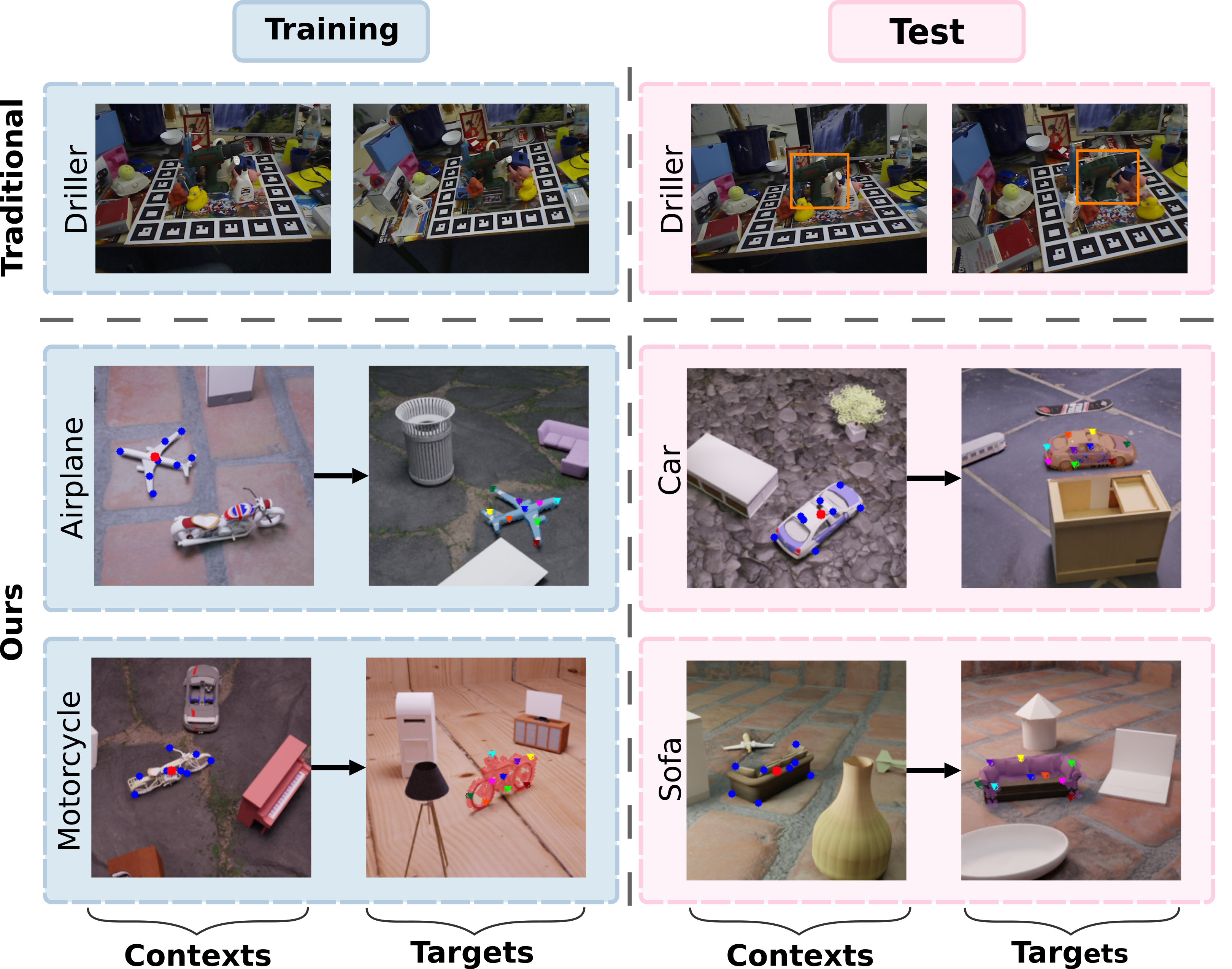
In this paper, we present a new meta-learning based approach to increase the generalization capability of 6D pose estimation. To our knowledge, this is the first work that allows generalization across object categories. The main idea of our method lies in meta-learning object-centric representations in a category-agnostic way. Meta-learning aims to adapt rapidly to new tasks based only on a few examples. More specifically, we employ Conditional Neural Processes (CNPs) [21] to learn a latent representation of objects, capturing the generic appearance and geometry. Inference on new objects then merely needs a few labeled examples as input to extract a respective representation. In particular, fine-tuning on new objects is not necessary. A comparison between traditional instance-level approaches and ours is illustrated in Fig. 1.

For feature extraction, we use FFB6D [26], which learns representative features through a fusion network based on RGB-D images. However, instead of directly using the extracted features for downstream applications, i.e., segmentation and keypoint offsets prediction, we add CNP on top of the fusion network to further meta-learn a latent representation for each object. CNP takes in the representative features from a set of context images of an object, together with their ground-truth labels, and yields a latent representation. The subsequent predictions for new target images are conditioned on this latent representation.

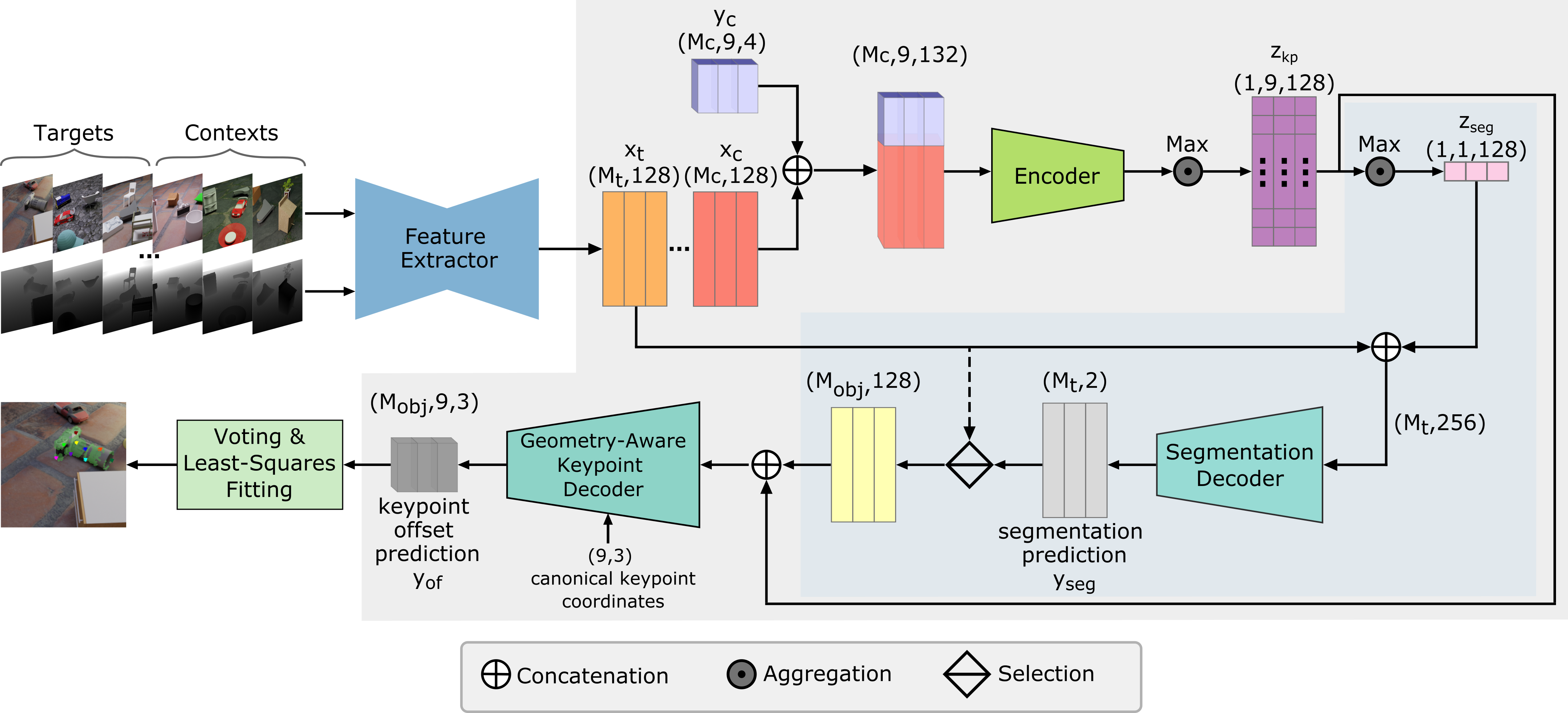
To further leverage the object geometry and improve the keypoint prediction, we propose a novel GNN-based decoder which takes predefined canonical keypoints in the object’s reference frame as an additional input and encodes local spatial constraints via message passing among the keypoints. Note that the additional input to the GNN does not require any further annotations on top of those existing datasets used by prior keypoint-based methods. The proposed pipeline is illustrated in Fig. 2.

Due to the lack of available data for cross-category level 6D pose estimation, we generate our own synthetic dataset for Multiple Categories in Multiple Scenes (MCMS) using objects from ShapeNet [3] and extending the open-source rendering pipeline [10] with online occlusion and truncation checks. This provides us with the flexibility to generate datasets with limited and considerable occlusion respectively.

Figure 2: Schematic pipeline of our approach.

In summary, the main contributions of this work are as follows:

• We introduce a novel meta-learning framework for 6D pose estimation with strong generalization ability on unseen objects within and across object categories.

• We propose a GNN-based keypoint prediction module that leverages geometric information from canonical keypoint coordinates and captures local spatial constraints among keypoints via message passing.

• We provide fully-annotated synthetic datasets with abundant diversity, which facilitate future research on intra- and cross-category level 6D pose estimation.

2 Related Work

6D Pose Estimation. For instance-level 6D pose estimation, methods can be categorized into three classes: correspondence-based, template-based and voting-based methods [11]. Correspondence-based methods aim to find 2D-3D correspondences [70, 54, 47] or 3D-3D correspondences [17]. Template-based methods, on the other hand, match the inputs to templates, which can be either explicit pose-aware images [28, 29] or templates learned implicitly by neural networks [56]. Voting-based approaches [45, 27, 26] generate voting candidates from feature representations, after which the RANSAC algorithm [18] or a clustering mechanism such as MeanShift [9] is applied for selecting the best candidates. Our feature extractor, FFB6D [26], falls into this latter category. FFB6D proposes a bidirectional fusion module to combine appearance and geometry information for feature learning. The extracted features are then used to predict per-point semantic labels and keypoint offsets, after which MeanShift is used to vote for 3D keypoints. Finally, the keypoints are used to predict the final 6D pose by Least-Squares Fitting [1].

Recently, category-level 6D object pose estimation has gained increasing attention [64, 4, 62, 7, 8]. Wang et al.  [64] share a canonical representation for all possible object instances within a category using Normalized Object Coordinate Space (NOCS). However, inferring the object pose by predicting only the NOCS representation is not easy given large intra-category variations [14]. To tackle this problem,  [58] accounts for intra-category shape variations by explicitly modeling the deformation from shape prior to object model while CASS [4] generates 3D point clouds in the canonical space using a variational autoencoder (VAE). FS-Net [7] proposes a shape-based model using 3D graph convolutions and a decoupled rotation mechanism to further reduce the sensitivity of RGB features to the color variations. However, these methods model the feature space explicitly on a category-level and therefore have a limited generalization ability across categories. By contrast, our method learns 6D pose estimation in a category-agnostic manner and can handle new objects from unseen categories.

Meta-Learning. Meta-learning, also known as learning to learn, aims to acquire meta knowledge that can help the model to quickly adapt to new tasks with very few samples. In general, meta-learning can be categorized into metric-based [60, 53, 57], optimization-based [15, 43, 16] and model-based [50, 21, 22, 32] methods. Many meta-learning approaches have been applied to computer vision applications, e.g., few-shot image classification [24, 71, 59, 39], vision regression [20], object detection [46, 12, 13, 72, 6], robotic grasping [19], semantic segmentation [52, 36, 44, 73] and 3D reconstruction [61, 42]. Our work is based on Neural Processes (NPs) [22, 32, 41, 25, 34], which fall into the category of model-based meta-learning approaches. NPs have shown promising performance on simple tasks like function regression and image completion. However, their application to 6D pose estimation has not yet been explored properly. We introduce CNP [21] to this problem in order to tackle the issue of poor generalization ability of existing methods on both intra- and cross-category level.

Graph Neural Networks. Graph neural networks (GNNs) have been widely applied on vision applications, such as image classification [35, 31, 40], semantic segmentation [49, 33, 66, 37], and object detection [30, 51, 67]. Recently, many works start using GNNs on human pose estimation [65, 2, 69]. Yang et al.  [69] derive the pose dynamics from historical pose tracklets through a GNN which accounts for both spatio-temporal and visual information while PGCN [2] builds a directed graph over the keypoints of the human body to explicitly model their correlations. DEKR [23] adopts a pixel-wise spatial transformer to concentrate on information from pixels in the keypoint regions and dedicated adaptive convolutions to further disentangle the representation. Our approach is based on a similar idea as PGCN, where we take the keypoints in the canonical object coordinates as an additional input in order to leverage the spatial constraints between keypoints. We show that this drastically increases the performance on unseen objects and robustness on occluded scenes.

3 Preliminary - Conditional Neural Processes

Conditional Neural Processes (CNPs) [21] can be interpreted as conditional models that perform inference for some target inputs $x_{t}$ conditioned on observations, called “contexts”. These contexts consist of inputs $x_{c}$ and corresponding labels $y_{c}$ originating from one specific task. Note that in our case, each distinct object is considered as a task.

The basic form of CNP comprises three core components: encoder, aggregator and decoder. The encoder takes a set of $M_{c}$ context pairs from a given task $C=\{(x_{c}^{i},y_{c}^{i})\}_{i=1}^{M_{c}}$ and extracts embeddings from each context pair respectively, $r_{i}=h_{\theta}(x_{c}^{i},y_{c}^{i}),\ \forall(x_{c}^{i},y_{c}^{i})\in C$, where $h$ is a neural network parameterized by $\theta$. Afterwards, the aggregator $a$ summarizes these embeddings using a permutation invariant operator $\otimes$ and yields the global latent variable as task representation: $z=a(r_{1},r_{2},...,r_{M_{c}})=r_{1}\otimes r_{2}\otimes...\otimes r_{M_{c}}$. Since the size of context set $M_{c}$ varies and the task representation has to be independent of the order of contexts, a permutation invariant mechanism is essential. Max aggregation is used in our model as we empirically find it outperforms mean aggregation, which is used in the original CNP. Finally, the decoder performs predictions for a set of target inputs $T=\{x_{t}^{i}\}_{i=1}^{M_{t}}$ conditioned on the corresponding task representation $z$ extracted and aggregated before: $\hat{y}_{t}^{i}=g_{\phi}(x_{t}^{i},z),\ \forall x_{t}^{i}\in T$. $M_{t}$ is the number of target inputs, $g$ denotes the decoder, a neural network parametrized by $\phi$.

The ability to extract meaningful latent representation from very few samples renders CNP well-suited for our purposes. Due to the fact that each distinct object comes with different predefined keypoints, prior keypoint-based methods for 6D pose estimation do not generalize well to novel objects. Meta-training CNP to extract latent keypoint representations from object features, however, allows us to overcome this difficulty.

4 Approach

In this paper, we propose a keypoint-based meta-learning approach for 6D pose estimation on unseen objects. Given an RGB-D image, the goal of 6D pose estimation is to calculate the rigid transformation $[R;t]$ from the object coordinates to the camera coordinates, where $R\in SO(3)$ represents the rotation matrix and $t\in\mathbb{R}^{3}$ represents the translation vector. We build on keypoint-based methods, that first predict the location of keypoints in camera coordinates from input RGB-D images and then regress the transformation between these and predefined keypoints in the object coordinates. The predefined keypoints in canonical object coordinates are thereby fixed beforehand, e.g., using the Farthest Point Sampling (FPS) algorithm on the object mesh.

Figure 3: Overview of the three stages of our method. a) The feature extractor takes RGB-D images as inputs and produces point-wise features for a set of $M_{c}$ ($M_{t}$) points subsampled from the input context (target) image. b) The meta-learner (grey shaded area) encodes and aggregates the features of several context images into two latent variables $z_{kp}$ and $z_{seg}$. The segmentation module (blue shaded area) predicts a binary semantic label for each of the $M_{t}$ feature points of a target image conditioned on the latent representations $z_{seg}$, indicating whether the respective point belongs to the queried object. The keypoint decoder predicts per-point offsets for each keypoint based on the segmented features and the keypoint latent variables $z_{kp}$. c) Lastly, 6D pose parameters are computed via voting and least-squares fitting.

4.1 Overview

We consider 6D pose estimation in three stages: feature extraction, keypoint detection and pose fitting. At the first stage, we employ the feature extractor FFB6D [26] to extract representative features from RGB-D images. For the second stage we use a CNP-based meta-learning approach. The flow of context and target samples through our model is shown in Fig. 3, where the context inputs for each task $x_{c}$, i.e., the features extracted from the context RGB-D images, and the correpsonding labels $y_{c}$ are used jointly to distill a task representation. This representation serves as prior knowledge for the subsequent prediction on target inputs $x_{t}$. We use two decoders in our meta-learning framework, predicting semantic labels and 3D keypoint offsets respectively. Furthermore, we propose a novel geometry-aware decoder using a GNN for the keypoint offsets prediction, which explicitly models the spatial constraints between the keypoints. Finally, the 6D pose parameters are regressed by least-squares fitting at the third stage.

4.2 Feature Extraction

For feature extraction we rely on the fusion network FFB6D [26] which combines appearance and geometry information from RGB-D images and extracts representative features for a subset of seed points sampled from the input depth images. Therefore, the output is a set of per-point features corresponding to the sampled seed points.

4.3 Meta-Learner for Keypoint Detection

Two steps are involved in the keypoint estimation procedure: segmentation of the queried object and keypoint detection, which both rely on a preceding extraction of latent representations.

Extraction of latent representations. Identifying and distinguishing a novel object from a multi-object scene and extracting its keypoints requires modules, which are conditioned on the latent representation of the queried object. In order to obtain such a latent representation, we need a set of context samples $\{(x_{c,i},y_{c,i})\}_{i=1}^{M_{c}}$. Here $x_{c,i}$ denotes the per-point features extracted in the first stage from context images and $y_{c,i}=\{y_{c,i}^{u}\}_{u=1}^{M_{K}}$ is the ground-truth label where $y_{c,i}^{u}=\{y_{of}^{u},y_{seg}\}_{c,i}$ includes the 3D keypoint offsets $y_{of}^{u}$ between the seed point and predefined keypoint $p_{u}$, and semantic label $y_{seg}\in\{0,1\}$ indicating whether the seed point belongs to the queried object. Given a context sample as input, an encoder generates per-seed-point embeddings for each of the $M_{k}$ keypoints to be predicted:

$$r_{i}^{u}=h_{\theta}(x_{c,i}\oplus y_{c,i}^{u}),\ i=1,...,M_{c},\ u=1,...,M_{k},$$ (1)

where $M_{c}$ denotes the number of seed points selected from each context image; $M_{k}$ is the number of selected keypoints which in our case is 9. $\oplus$ stands for the concatenation operation, where the inputs are first broadcast to the same shape, if necessary. The obtained embeddings are next aggregated by max aggregation to first obtain a latent representation $z_{kp}^{u}$ for each keypoint. A second aggregation over these keypoint representations is then applied in order to extract a representation $z_{seg}$ for the segmentation task:

$$z_{kp}^{u}=\max\limits_{i=1}^{M_{c}}(r_{i}^{u}),\ u=1,...,M_{k},$$ (2)

$$z_{seg}=\max\limits_{u=1}^{M_{k}}(z_{kp}^{u}).$$ (3)

Conditional Segmentation. In the step described above, the model encapsulates relevant information (e.g., shape and texture attributes) into the latent variable $z_{seg}$. This can then be used to identify and locate the queried object in the target images. The segmentation decoder $g_{\mathcal{S}}$ takes the latent variable $z_{seg}$ and features $x_{t}$ extracted from the target images (see Fig. 3) and predicts a semantic label for each seed point via a multi-layer perceptron (MLP):

$$y_{seg,i}=g_{\mathcal{S}}(x_{t,i}\oplus z_{seg}),\ i=1,...,M_{t},$$ (4)

where $M_{t}$ is the number of seed points sampled from each target image, $x_{t,i}$ denotes the corresponding extracted features. These per-point segmentation predictions $y_{seg}$ are then used to select only the seed point features $x_{obj}$ belonging to the queried object from $x_{t}$ for the subsequent keypoint prediction.

Conditional Keypoint Offset Prediction. The keypoint offsets decoder $g_{\mathcal{K}}$ takes the features extracted by the segmentation module along with the latent variables $z_{kp}$ as input and predicts translation offsets $y_{of}$ for each keypoint:

$$y_{of,i}^{u} =g_{\mathcal{K}}(x_{obj,i}\oplus z_{kp}^{u}),$$

$$i=1,...,M_{obj},\ u=1,...,M_{k},$$ (5)

where $M_{obj}$ denotes the number of selected seed points on the queried object, $x_{obj,i}$ denotes the object features of $i$-th seed point. The decoder $g_{\mathcal{K}}$ can be any appropriate module in Sec. 4.3. In the vanilla version of our framework, it is given by a trivial MLP. However, we use a GNN for $g_{\mathcal{K}}$ in our final version, the details of which will be given in Sec. 4.4.

Pose Fitting. Similar as in  [26], we adopt MeanShift [9] to obtain the final keypoint prediction $\{p_{i}^{*}\}_{i=1}^{M_{k}}$ in the camera coordinates, based on keypoint candidates output by the keypoint decoder. Given predefined 3D keypoints in object coordinates $\{p_{i}\}_{i=1}^{M_{k}}$, 6D pose estimation can be converted into a least-squares fitting problem [1] where the optimized pose parameters $[R;t]$ are calculated by minimizing the squared loss using singular value decomposition(SVD):

$$L_{lsf}=\sum_{i=1}^{M_{k}}\left\lVert p_{i}^{*}-(R\cdot p_{i}+t)\right\rVert^{2}.$$ (6)

4.4 Geometry-Aware Keypoint Decoder

Similar to prior methods [27, 26], we rely on predefined object keypoints for the final pose fitting. However, we also utilize them as an additional input to the keypoint decoder. Since they contain useful prior knowledge of the object’s geometric structure, they can significantly improve keypoint detection. In order to highlight the additional input to our decoder, we rewrite Sec. 4.3 as follows:

$$y_{of,i}^{u} =g_{\mathcal{K}}(x_{obj,i},\,z_{kp}^{v},\,p_{v}),\ v\in\mathcal{N}(u),$$ (7)

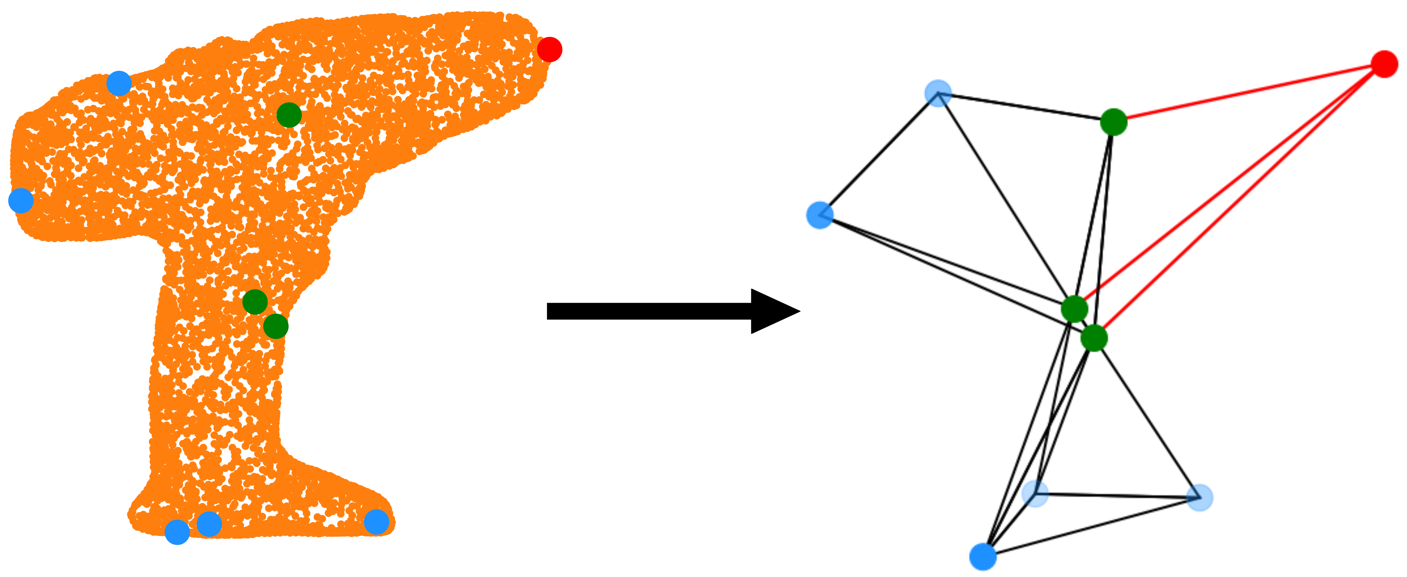
where $\mathcal{N}(u)$ denotes the neighbor set of keypoint $u$ including $u$ itself and $p_{v}$ are the 3D object coordinates of keypoint $v$. To leverage the geometric information contained in the relation among the keypoints, we propose a GNN-based decoder $g_{\mathcal{K}}$ instead of the trivial MLP in Sec. 4.3. For this purpose, we create a graph over the keypoints of each object. The nodes are given by the keypoints which share edges with their $k$ nearest neighbours. Fig. 4 illustrates an example with $k=3$.

Figure 4: Example of the graph generation. The node positions are determined by the predefined keypoints in object coordinates. By applying the K Nearest Neighbor (KNN) algorithm, we find the k closest adjacent nodes of each parent node and connect them by edges. For instance, the given graph is generated with $k=3$, where the red node is selected as the parent node and green nodes are the three nearest neighbors. The driller is sampled from LineMOD.

Internally, Eq. 7 is split into the following two steps involved in message passing along the graph:

$$\alpha_{i}^{u,v}=f^{l}(x_{obj,i}\oplus z_{kp}^{v},p_{u}-p_{v}),\ \forall v\in\mathcal{N}(u),$$ (8)

$$y_{of,i}^{u}=f^{g}(\max_{v\in\mathcal{N}(u)}\ \alpha_{i}^{u,v}).$$ (9)

$g_{\mathcal{K}}$ is correspondingly composed of two sub-networks, $f^{l}$ and $f^{g}$. These correspond to updating the messages $\alpha_{i}^{u,v}$ sent along all edges, aggregating the messages arriving at each node $u$ to update the corresponding node features and decoding them into keypoint offsets $y_{of,i}^{u}$.

5 Experiments

5.1 Datasets

(a) Toy

(b) PBR

(c) Occlusion

Figure 5: Samples from MCMS dataset.

Figure 6: Qualitative comparison between GNN and MLP decoder for keypoints prediction on PBR-MCMS. Triangles and circles are the projected ground-truth and predicted keypoints respectively. The keypoint predictions of the MLP decoder are randomly shifted without considering geometric constrains between keypoints. By contrast, the predictions by the GNN decoder are more accurate. The example of the motorcycle shows that though the keypoints predicted by the GNN are slightly shifted here, the geometric constraints are met, resulting in a uniform shift of all keypoints.

LineMOD. LineMOD [29] is a widely used dataset for 6D pose estimation which comprises 13 different objects in 13 scenes. Each scene contains multiple objects, but only one of them is annotated with a 6D pose and instance mask.

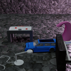
MCMS dataset. Due to the unavailability of datasets for cross-category level 6D pose estimation, we generate two fully-annotated synthetic datasets using objects from ShapeNet [3], which contain various objects from Multiple Categories in Multiple Scenes (MCMS). The simple version of MCMS, named Toy-MCMS, is composed of images containing a single object with backgrounds randomly sampled from the real-world image dataset SUN  [55]. Our second dataset can be further divided into a non-occluded and an occluded version, called PBR-MCMS and Occlusion-MCMS. To create these datasets, we extend the open-source physics-based rendering (PBR) pipeline [10] with functionalities such as online truncation and occlusion checks. For each image, five objects are placed in a random scene with textured planes and varying lighting conditions. Images are then photographed with a rotating camera from a range of distances. PBR-MCMS contains images without occlusion while Occlusion-MCMS contains images with $5\%-20\%$ occlusion of the queried object. Fig. 5 shows an example for each dataset using an object from the car category as the queried object.

5.2 Evaluation Metrics

We use the average distance metrics ADD [29] for evaluation. Given the predicted 6D pose $[R;t]$ and the ground-truth pose $[R^{*};t^{*}]$, the ADD metric is defined as:

$$\mathrm{ADD}=\frac{1}{m}\sum_{x\in\mathcal{O}}\left\lVert(Rx+t)-(R^{*}x+t^{*})\right\rVert,$$ (10)

where $\mathcal{O}$ denotes the object mesh and $m$ is the total number of vertices on the object mesh. This metric calculates the mean distance between the two point sets transformed by predicted pose and ground-truth pose respectively. Similar to other works [68, 45, 26], we report the ADD-0.1d accuracy, which indicates the ratio of test samples, where the ADD is less than 10% of the object’s diameter.

5.3 Implementation and Training Details

For each object, we define 9 keypoints, where 8 keypoints are sampled from the 3D object model using FPS, and the other one is the object center. The nearest neighbors used for each keypoint is set to $k=8$ in our geometry-aware decoder. To train the meta-learner, we use the Focal Loss [38] to supervise the segmentation module and a L1 loss for per-point translation offset prediction. The overall loss is weighted sum of both terms, with a weight 2.5 for segmentation and 1.0 for keypoint offsets. During training, for each iteration, we arbitrarily sample 18 objects and 12 images per object. The number of context images is randomly chosen between 2 and 8 per object while the remaining images are used as target set.

Training setup. For the LineMOD dataset, we use iron, lamp, and phone as novel objects for testing and the 10 remaining objects for training. Since LineMOD contains only a very limited number of objects, we only evaluate the keypoint offset prediction module using the ground-truth segmentation for selecting the points belonging to the queried object. For Toy- and PBR-MCMS, we use 20 and 19 categories for training respectively, with 30 objects per category and 50 images per object. During evaluation, 30 novel objects of each training category are tested for intra-categorical performance and 5 novel categories for cross-category performance. All experiments are conducted on NVIDIA V100-32GB GPU.

	Vanilla-ML	GAML
Category	ADD	ADD
Airplane	80.6	87.2
Bench	56.7	72.3
Chair	62.8	80.9
Motorcycle	92.6	94.7
Washer	85.4	91.4
Bus*	83.0	85.4
Cap*	46.6	54.2
Laptop*	18.8	48.8
Piano*	47.1	50.7
Remote*	53.5	56.1
Intra-Categ.	74.2	81.9
Cross-Categ.	50.3	59.0
All	69.4	77.2

Table 1: Multi-category evaluation on Toy-MCMS dataset. Novel objects are marked with *.

	FFB6D	Vanilla-ML			GAML
Category	PBR	PBR	Occ.	$\Delta$	PBR	Occ.	$\Delta$
Airplane	9.1	90.4	43.2	47.2	89.8	46.6	43.2
Bench	2.9	62.1	40.4	21.7	69.8	49.0	20.8
Chair	1.1	80.0	54.4	25.6	80.0	55.6	22.4
Motorcycle	12.7	90.2	64.8	25.4	85.6	54.4	31.2
Washer	4.1	54.8	37.7	17.1	68.1	55.0	13.1
Birdhouse*	0.8	35.6	23.5	12.1	35.4	28.0	7.4
Car*	2.4	52.5	42.9	9.6	56.9	44.4	12.5
Laptop*	1.3	54.0	26.0	28.0	85.0	47.7	37.3
Piano*	2.0	45.8	27.3	18.5	45.8	32.5	13.3
Sofa*	2.6	68.1	45.4	22.7	69.8	57.9	11.9
Intra-Categ.	4.53	58.2	38.7	19.5	62.9	43.9	19.0
Cross-Categ.	1.81	51.2	33.0	18.2	58.6	42.1	16.5
All	3.96	56.7	37.6	19.1	62.0	43.5	18.5

Table 2: Multi-category evaluation on PBR- and Occlusion-MCMS datasets. $\Delta$ represents the performance gap between PBR- and Occlusion-MCMS.

	FFB6D		Ours
Object	L1 Loss	ADD	L1 Loss	ADD
Ape	0.06	100	0.02	100
Holepuncher	0.07	100	0.02	100
Iron*	1.39	0.6	0.26	36.2
Lamp*	1.52	0.5	0.38	22.4
Phone*	0.89	0.0	0.17	17.8

Table 3: Evaluation results on LineMOD dataset.

5.4 Evaluation Results

We evaluate our approach using the LineMOD and MCMS datasets at intra- and cross-category levels. More quantitative and qualitative results are provided in Appendix A.

LineMOD. Tab. 3 shows training and test results following  [26]. Note that the segmentation ground-truth is used for these results and we only evaluate the performance and generalization ability of the keypoint offset prediction module. Our model not only performs better on training objects, but also generalizes well to new objects even though it is trained on a limited number of objects and tested on new objects with large variations in appearance and geometry.

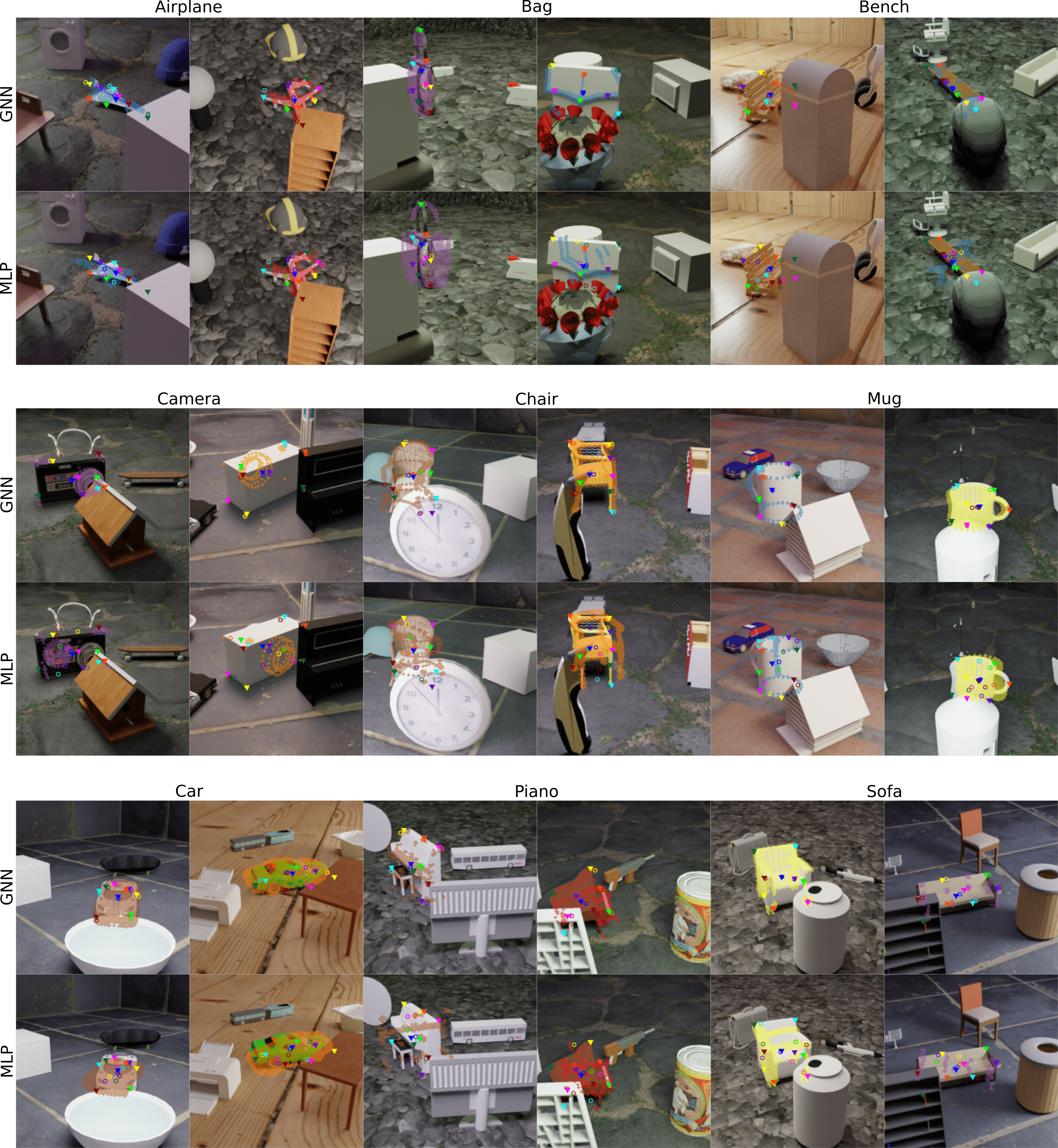
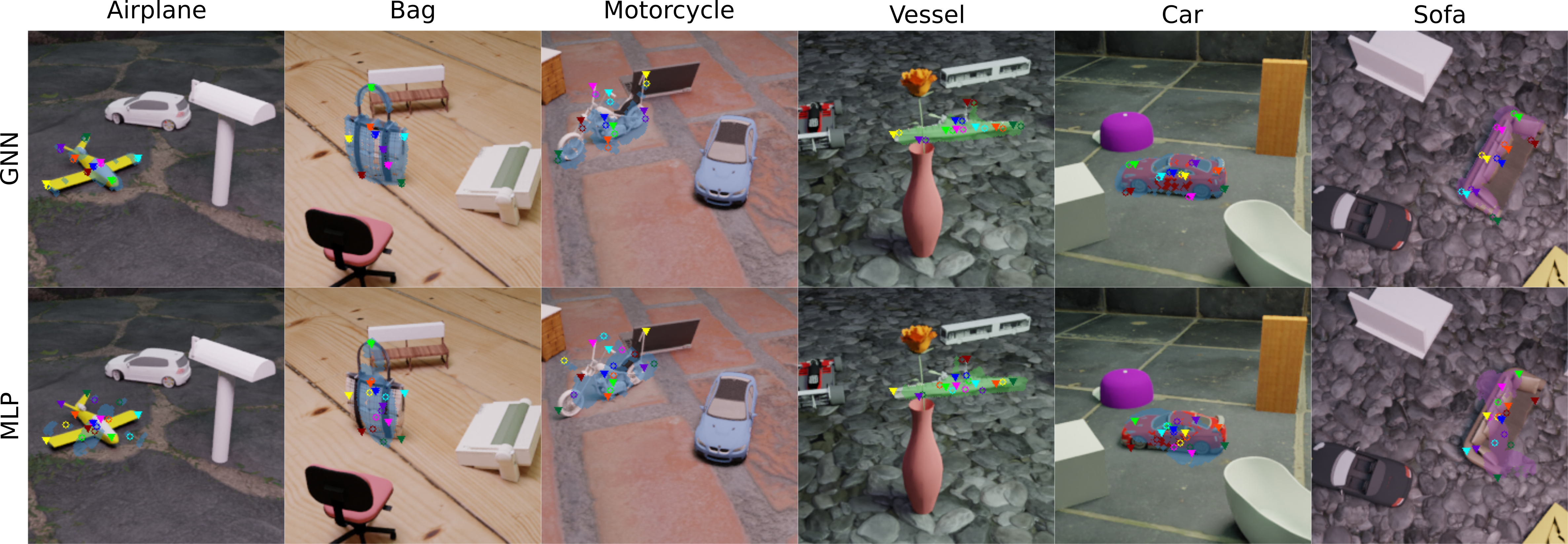
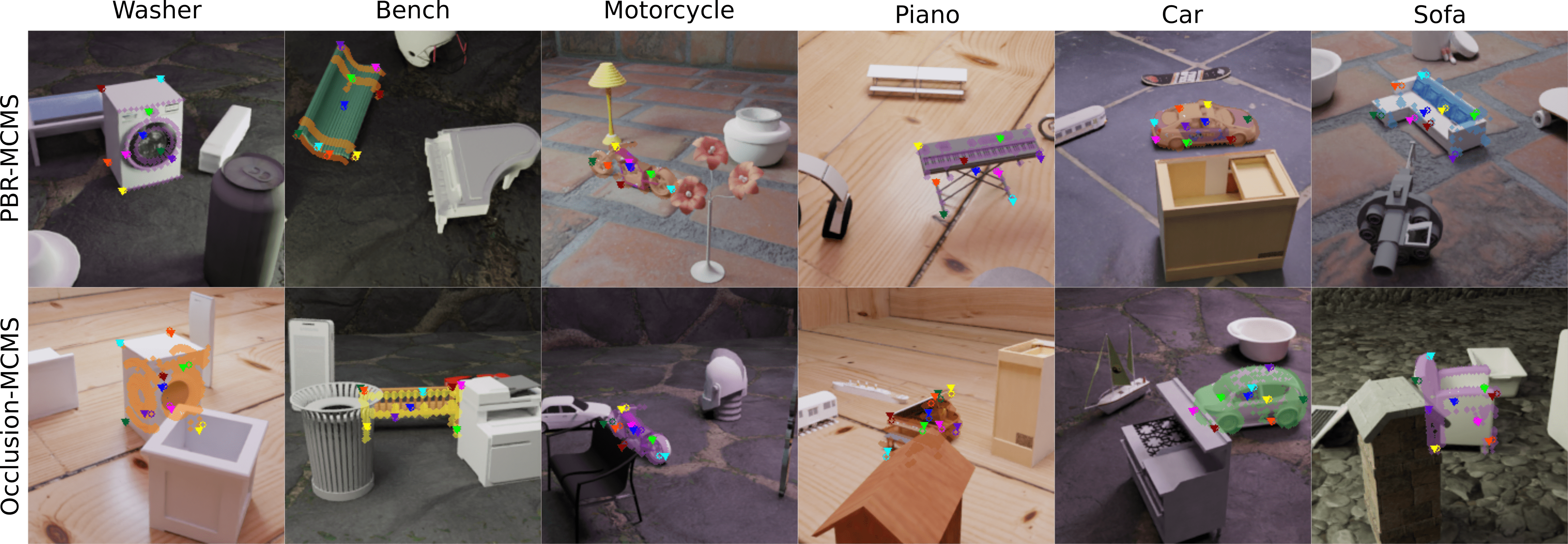
Toy- & PBR-MCMS. Tab. 2 shows test results on the Toy-MCMS dataset, which demonstrate that our proposed GNN decoder (GAML) consistently outperforms the Vanilla Meta Learner (Vanilla-ML) using classic MLP decoder on all categories. Fig. 6 visualizes some test examples for qualitative comparison. Next, we compare our meta-learner to FFB6D on the PBR dataset. Tab. 2 shows that our model generalizes well while FFB6D cannot directly transfer to novel objects. For a fair comparison, we further train FFB6D on the PBR dataset and fine-tune the pretrained model on each specific novel object with the same context images as given to GAML. Tab. 4 shows that our model still outperforms the fine-tuned FFB6D reliably and requires no trade-off between new and preceding tasks, whereas fine-tuning normally leads to a performance decrease on the previous tasks.

	Airplane	Chair	Car	Laptop	Sofa
FFB6D	60.0	52.0	36.7	48.0	49.3
GAML	89.8	80.0	56.9	85.0	69.8

Table 4: Comparison between GAML and fine-tuned FFB6D on PBR-MCMS using ADD metric.

Figure 7: Qualitative results on PBR- and Occlusion-MCMS datasets. Triangles and circles are the projections of ground-truth and predicted keypoints respectively. Note that our model is trained only on PBR-MCMS but shows robust performance on Occlusion-MCMS.

Occlusion-MCMS. Quantitative and qualitative results on Occlusion-MCMS are presented in Tab. 2 and Fig. 7. Strikingly, our approach achieves consistent and robust performance on occluded scenes even though training is conducted on non-occluded PBR-MCMS.

5.5 Ablation Study

Effect of K Neighbors in GNN. In Tab. 5, we study the effect of the $k$ neighbors in the GNN. We run tests using five seeds and calculate the mean. Compared to $k=3$, using all keypoints as neighbors can improve the robustness. We find this to be more crucial when training on a single category with limited object variations, where involving all keypoints gives more expressive spatial representation. Full statistics are presented in Sec. B.1.

	k = 3	k = 8
Multi-Categ.	60.1	61.9
Single-Categ.	77.9	83.3

Table 5: ADD Results on PBR-MCMS using different number $k$ of neighbors in GNN decoder.

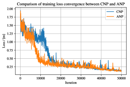
Effect of the Aggregation Module in CNP. In our work, CNP uses max aggregation instead of mean as used in the original paper [21]. We further compare max aggregation with the cross-attention module proposed in Attentive Neural Processes (ANPs) [32] removing the self-attention part. The training curves (see Sec. B.2) show that both methods achieve similar training performance, though ANP converges faster at the beginning. Nevertheless, Tab. 6 illustrates that CNP generalizes slightly better to novel tasks on both intra- and cross-category levels.

Robustness to Occlusion. To further illustrate the benefits coming from the geometry-aware estimator, we compare GAML with Vanilla-ML. The results in Tab. 2 show that our purposed GNN decoder significantly improves the performance and robustness on occluded scenes.

	Intra-Categ.	Cross-Categ.	All
CNP	81.9	59.0	77.2
ANP	80.8	58.1	76.3

Table 6: ADD Results of CNP and ANP on Toy dataset.

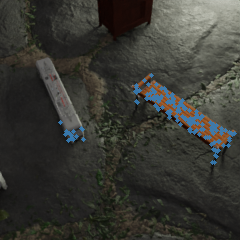
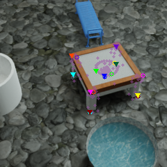
Limitations. We find two limitations of our method. First, we observe that in rare cases, our model suffers from Feature Ambiguity by struggling to disentangle feature variations, e.g., textures, shapes and lighting conditions. Sometimes it can be fooled by two similar objects which results in inaccurate segmentation (see Fig. 8(a)). Second, keypoint-based approaches suffer from Symmetry Ambiguity, especially on novel objects where the symmetric axis is unknown. Consequently, keypoint predictions around the symmetric axis can be mismatched and hamper the training (see Fig. 8(b)). Accounting for the symmetry ambiguity, we also provide evaluations with the ADD-S metric in Sec. A.3 following prior work [26, 63, 27].

(a) Feature ambiguity.

(b) Symmetry ambiguity.

Figure 8: Limitations of the proposed method.

6 Conclusion

In this paper, we present a CNP-based meta-learner for cross-category level 6D pose estimation, which is capable of extracting and transferring latent representation on unseen objects from only a few samples. Besides, we propose a simple yet effective geometry-aware keypoint detection module using GNN, which leverages the spatial connections between keypoints and improves generalization on unseen objects and robustness on occluded scenes. Furthermore, we create fully-annotated synthetic datasets called MCMS with various objects and categories, aiming to fill the vacancy for cross-category pose estimation.

Appendix A Evaluation Results

We present evaluation results on both LineMOD and MCMS datasets. More results and code are available at https://github.com/Cvpr2022ID5164/CVPR2022-ID5164.

A.1 LineMOD Dataset

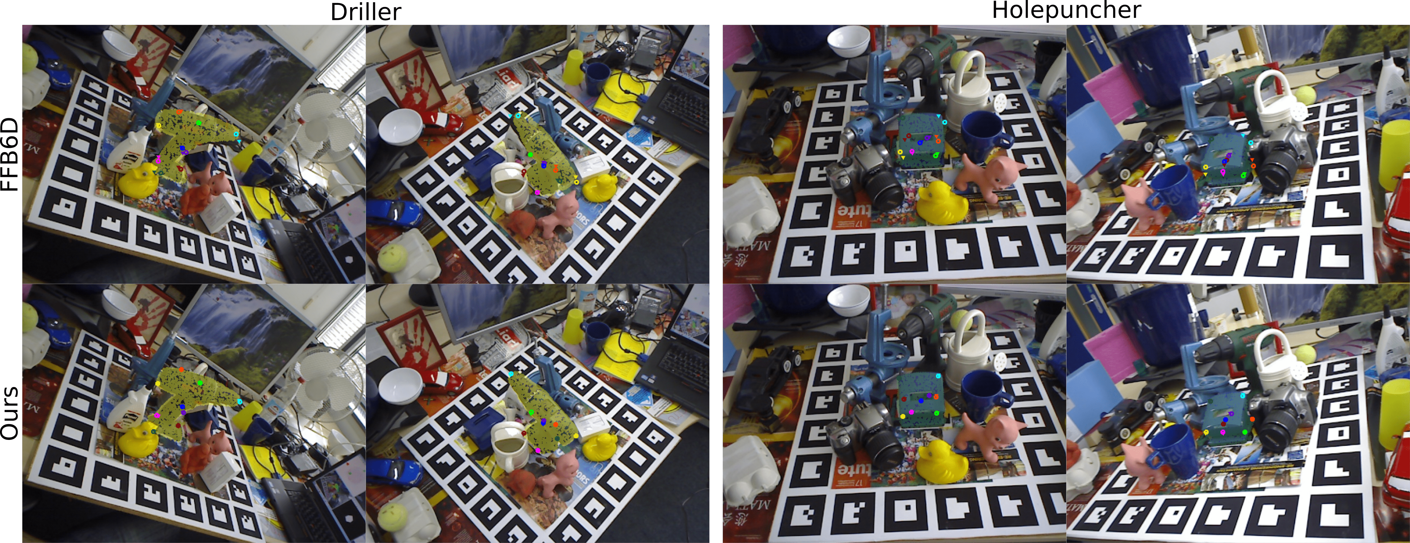
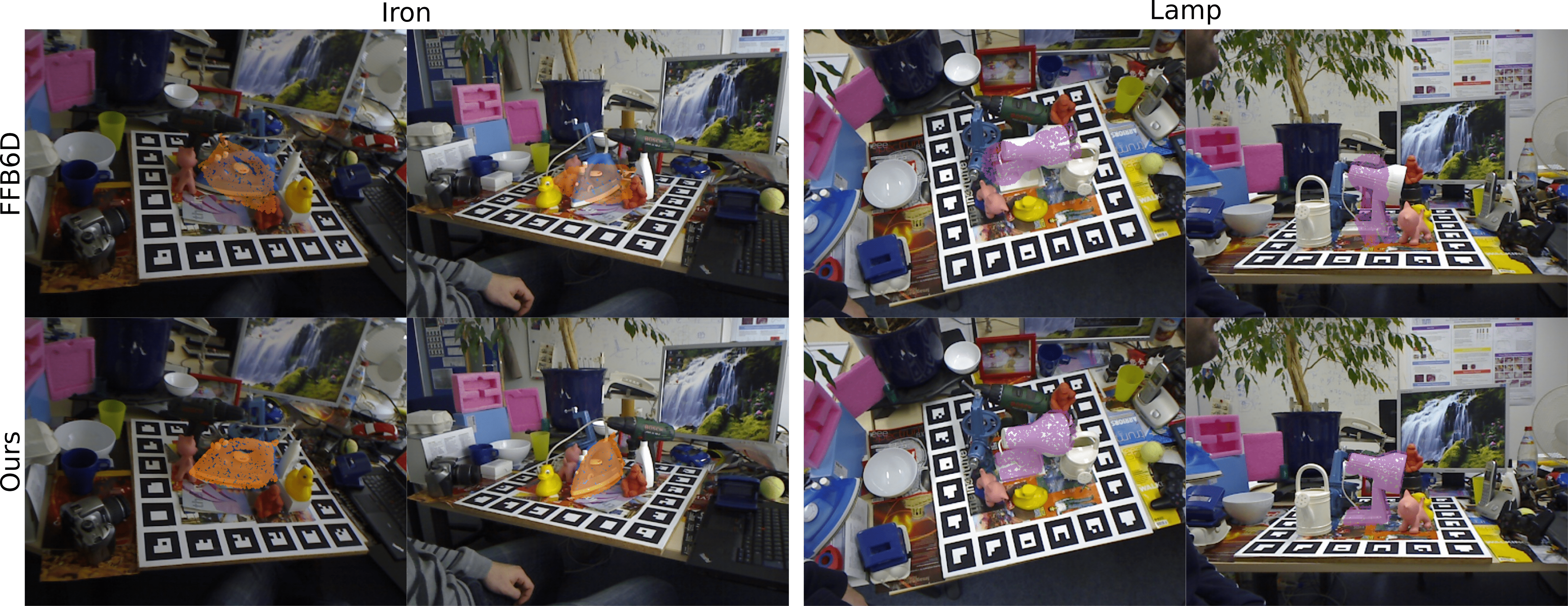
The LineMOD dataset [29] is split into 10 training objects and 3 unseen test objects, where iron, lamp and phone are the novel test objects. Fig. 2 show the qualitative comparison between FFB6D [26] and the proposed model on training objects. It can be observed that our model can predict keypoints more accurately. From Fig. 3, we can see that our model achieves better performance on novel objects. It should be noted that we only train one model for all objects, rather than train one model for each object respectively.

A.2 Toy-MCMS Dataset

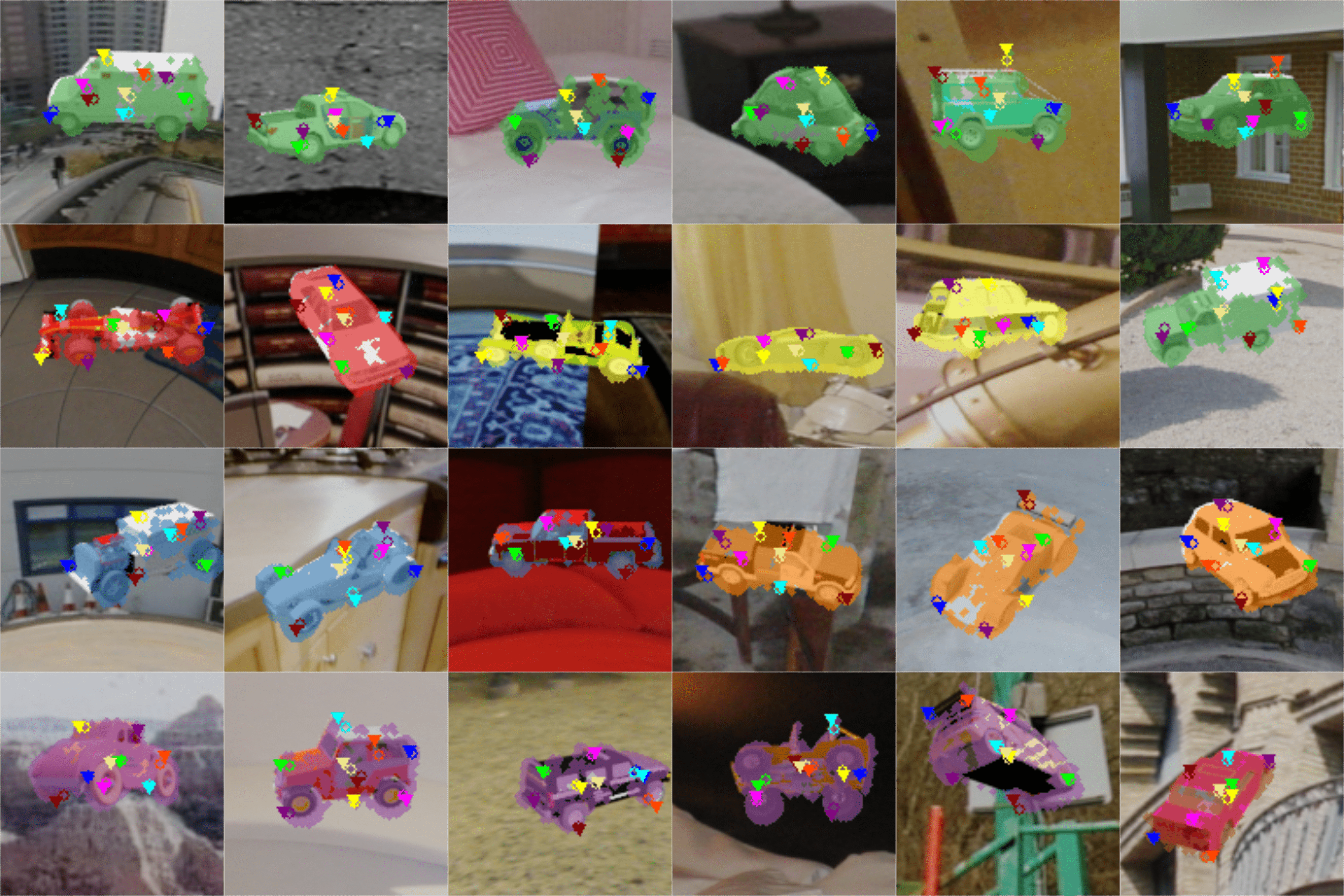
Tab. 1 provides the quantitative results of inter-category 6D pose estimation on the car category. We use 50 images per object for training and vary the number of training objects. From the experimental results, 80 car objects can achieve a similar ADD accuracy as 1100 objects, while the training time is reduced evidently. Overall, this represents a good comprise between prediction performance and training overhead. Fig. 4 shows the qualitative results on novel test objects using the model trained with 80 objects. Note that even within the car category, the colors and shapes of novel objects still vary a lot.

#Training objects	L1 loss[m]	ADD-0.1d[%]	Time[h]
1100	0.128	98.7	159
80	0.245	96.7	16

Table 1: Single category - car evaluation on Toy-MCMS dataset

Tab. 2 shows the quantitative results of the multi-category evaluation on the Toy-MCMS dataset. The vanilla meta-learner (Vanilla-ML) using MLP decoder is compared with the proposed geometry-aware meta-learner (GAML). It is obvious that GAML outperforms the Vanilla-ML by a large margin.

	Vanilla-ML		GAML
Category	L1 Loss	ADD-0.1d	L1 Loss	ADD-0.1d
Airplane	0.41	80.6	0.33	87.2
Bag	0.34	85.2	0.30	87.1
Basket	0.83	49.7	0.62	65.1
Bathtub	0.46	79.3	0.34	88.6
Bed	0.72	60.1	0.57	72.0
Bench	0.95	56.7	0.63	72.3
Birdhouse	0.35	83.2	0.28	89.7
Bookshelf	0.48	79.5	0.42	80.9
Cabinet	0.39	83.5	0.31	89.7
Car	0.31	92.9	0.28	92.9
Camera	0.57	65.0	0.46	73.4
Chair	0.57	62.8	0.42	80.9
Helmet	0.46	69.8	0.43	80.9
Motorcycle	0.29	92.6	0.25	94.7
Mug	0.25	91.9	0.24	93.3
Pillow	0.76	54.7	0.58	81.5
Table	0.80	61.1	0.54	76.2
Train	0.41	80.6	0.36	86.2
Vessel	0.62	66.9	0.53	70.9
Washer	0.36	85.4	0.28	91.4
Bus*	0.46	83.0	0.42	85.4
Cap*	0.71	46.6	0.64	54.2
Laptop*	1.02	18.8	0.73	48.8
Piano*	0.86	47.1	0.75	50.7
Remote*	0.53	53.5	0.52	56.1
Intra-Categ.	0.52	74.2	0.41	81.9
Cross-Categ.	0.72	50.3	0.62	59.0
All	0.56	69.4	0.45	77.2

Table 2: Multi-category evaluation on Toy-MCMS dataset

A.3 PBR-MCMS Dataset

We compare FFB6D, Vanilla-ML and GAML on intra- and cross-category levels. The full statistical summary can be found in Tab. 6. In general, the ADD metric is used for non-symmetric objects and ADD-S [29] for symmetric objects. Since the matching between points is ambiguous for some poses, ADD-S computes the mean distance based on the minimum point distance:

$$\mathrm{ADD-S}=\frac{1}{m}\sum_{x_{1}\in\mathcal{O}}\min_{x_{2}\in\mathcal{O}}\left\lVert(Rx+t)-(R^{*}x+t^{*})\right\rVert.$$ (1)

A.4 Occlusion-MCMS Dataset

Comparison between Vanilla-ML and GAML on Occlusion-MCMS is given in Tab. 3.

	Vanilla-ML		GAML
Category	L1 Loss	ADD-0.1d	L1 Loss	ADD-0.1d
Airplane	0.93	43.2	0.69	46.6
Bag	0.46	29.4	0.54	39.6
Bathtub	0.66	29.6	0.76	34.0
Bed	0.48	53.3	0.71	44.2
Bench	0.66	40.4	0.67	49.0
Bookshelf	0.38	42.5	0.49	42.7
Bus	0.67	37.5	0.55	47.5
Cabinet	0.48	35.2	0.44	55.2
Camera	0.45	39.4	0.45	40.4
Cap	0.39	42.1	0.45	43.1
Chair	0.36	54.4	0.32	55.6
Earphone	0.44	24.1	0.56	35.6
Motorcycle	0.37	64.8	0.40	54.4
Mug	0.38	40.2	0.34	52.9
Table	0.62	23.3	0.72	29.4
Train	0.52	32.3	0.53	36.2
Vessel	0.60	40.3	0.90	33.4
Washer	0.46	37.7	0.44	55.0
Printer	0.56	27.5	0.57	39.6
Birdhouse*	0.44	23.5	0.51	28.0
Car*	0.52	42.9	0.50	44.4
Laptop*	0.47	26.0	0.41	47.7
Piano*	0.51	27.3	0.66	32.5
Sofa*	0.48	45.4	0.44	57.9
Intra-Categ.	0.52	38.7	0.55	43.9
Cross-Categ.	0.48	33.0	0.51	42.1
All	0.51	37.6	0.54	43.5

Table 3: Multi-category evaluation on Occlusion-MCMS dataset

Appendix B Ablation Study

B.1 Effect of K Neighbors in GNN

We measure the ADD-0.1d accuracy of multi-category and single-category training with $k=3$ and $k=8$ in the GNN decoder. Tab. 4 presents the quantitative results.

		k = 3	k = 8
Multi.	Intra-Categ.	60.1	62.9
	Cross-Categ.	60.2	58.3
	All	60.1	61.9
Single.	Airplane	89.1	93.4
	Bathtub	43.8	46.9
	Bench	74.0	75.6
	Camera	67.0	69.6
	Car	90.6	94.6
	Chair	93.3	88.6
	Laptop	99.6	99.1
	Motorcycle	94.4	94.4
	Piano	74.7	98.1
	Sofa	91.2	96.6
	Vessel	45.7	69.0
	Washer	72.7	73.5
	Mean	77.9	83.3

Table 4: Effect of $K$ neighbors in GNN decoder on PBR-MCMS. The first block provides the statistic for multi-category training, where one model is trained on multiple categories and tested on new objects of both training and new categories. For single category training, each model is trained and tested per category.

B.2 Effect of Aggregation Module in CNP

Fig. 1 shows that both CNP and ANP methods achieve similar training performance in the end, even though ANP converges faster at the beginning.

Figure 1: Comparison of training loss between CNP and ANP

Appendix C Network Architecture

The detailed architecture model is shown in Tab. 5. We use ReLU as activation function after each FC layer except the output layer of segmentation decoder and global GNN decoder for keypoint offset prediction.

Component	Layer	Output Size
Encoder	FC	128
	FC	128
	FC	128
Seg. Decoder	FC	128
	FC	128
	FC	128
	FC	2
Local GNN	FC	128
	FC	128
	FC	128
Global GNN	FC	128
	FC	128
	FC	3

Table 5: GAML network architecture.

	FFB6D			Vanilla-ML			GAML
Category	L1 Loss	ADD	ADD-S	L1 Loss	ADD	ADD-S	L1 Loss	ADD	ADD-S
Airplane	1.51	9.1	85.7	0.11	90.4	96.8	0.11	89.8	98.8
Bag	1.98	5.1	48.1	0.41	40.0	85.0	0.47	42.7	87.1
Bathtub	2.22	2.7	41.4	0.55	43.3	86.7	0.60	45.2	90.8
Bed	2.31	2.9	33.3	0.31	72.3	90.4	0.41	58.5	90.8
Bench	2.26	2.9	43.0	0.39	62.1	91.4	0.35	69.8	91.7
Bookshelf	2.28	2.4	32.6	0.36	55.0	85.4	0.41	50.2	77.9
Bus	1.94	3.5	56.5	0.51	41.5	89.6	0.36	69.8	92.7
Cabinet	2.38	2.2	24.0	0.43	53.5	73.7	0.34	67.7	83.5
Camera	1.93	2.1	51.5	0.38	46.3	86.3	0.34	54.8	85.8
Cap	1.75	3.1	68.5	0.19	79.2	98.5	0.19	80.8	98.8
Chair	2.27	1.1	26.1	0.18	80.0	93.1	0.19	80.0	89.6
Earphone	1.79	4.2	62.8	0.38	34.0	86.2	0.43	49.2	97.1
Motorcycle	1.65	12.7	85.1	0.16	90.2	98.5	0.21	85.6	98.1
Mug	2.08	0.9	43.7	0.12	86.8	97.9	0.14	84.2	94.4
Table	2.38	2.0	19.2	0.61	33.1	73.5	0.65	39.2	93.1
Train	1.67	12.9	71.9	0.46	38.5	85.8	0.49	47.7	90.6
Vessel	1.64	11.0	68.9	0.35	57.7	94.1	0.37	56.0	90.4
Washer	2.48	4.1	29.1	0.33	54.8	85.4	0.30	68.1	89.0
Printer	2.21	1.0	33.1	0.41	47.9	83.9	0.43	55.2	80.0
Birdhouse*	2.09	0.8	21.0	0.39	35.6	59.4	0.43	35.4	64.6
Car*	1.79	2.4	70.5	0.44	52.5	97.1	0.43	56.9	96.7
Laptop*	2.22	1.3	10.5	0.32	54.0	82.9	0.20	85.0	93.1
Piano*	2.04	2.0	39.3	0.43	45.8	77.5	0.44	45.8	80.0
Sofa*	2.17	2.6	27.1	0.34	68.1	84.6	0.34	69.8	79.0
Intra-Categ.	2.03	4.53	48.7	0.35	58.2	88.5	0.36	62.9	90.0
Cross-Categ.	2.06	1.81	33.7	0.38	51.2	80.2	0.37	58.6	82.7
All	2.04	3.96	45.5	0.36	56.7	86.8	0.36	62.0	88.4

Table 6: Multi-category evaluation on PBR-MCMS dataset

Figure 2: Qualitative comparison on trained LineMOD objects. Triangles and circles are the projections of ground-truth and predicted keypoints respectively. It can be observed that keypoint predictions of our method are more accurate.

Figure 3: Qualitative comparison on new LineMOD objects. Compared with FFB6D, the pose estimation on new objects of our GAML model is more accurate.

Figure 4: Qualitative results on Toy-MCMS. Our model can handle large intra-category variations. The car category is illustrated as an example.

Figure 5: Qualitative comparison between GNN and MLP decoder on Occlusion-MCMS. Triangles and circles are the projected ground-truth and predicted keypoints respectively.

References

- [1] K. S. Arun, T. S. Huang, and S. D. Blostein. Least-squares fitting of two 3-d point sets. IEEE Transactions on Pattern Analysis and Machine Intelligence, PAMI-9(5):698–700, 1987.
- [2] Yanrui Bin, Zhao-Min Chen, Xiu-Shen Wei, Xinya Chen, Changxin Gao, and Nong Sang. Structure-aware human pose estimation with graph convolutional networks. Pattern Recognition, 106:107410, 05 2020.
- [3] Angel X. Chang, T. Funkhouser, L. Guibas, P. Hanrahan, Qixing Huang, Zimo Li, S. Savarese, M. Savva, Shuran Song, Hao Su, J. Xiao, L. Yi, and F. Yu. Shapenet: An information-rich 3d model repository. ArXiv, abs/1512.03012, 2015.
- [4] Dengsheng Chen, Jun Li, Zheng Wang, and Kai Xu. Learning canonical shape space for category-level 6d object pose and size estimation. In IEEE/CVF Conference on Computer Vision and Pattern Recognition (CVPR), June 2020.
- [5] Kai Chen and Qi Dou. Sgpa: Structure-guided prior adaptation for category-level 6d object pose estimation. In Proceedings of the IEEE/CVF International Conference on Computer Vision (ICCV), pages 2773–2782, October 2021.
- [6] Tung-I Chen, Yueh-Cheng Liu, Hung-Ting Su, Yu-Cheng Chang, Yu-Hsiang Lin, Jia-Fong Yeh, and Winston H. Hsu. Should I look at the head or the tail? dual-awareness attention for few-shot object detection. IEEE Trans. Multim., 23, 2021.
- [7] Wei Chen, Xi Jia, Hyung Jin Chang, Jinming Duan, Linlin Shen, and Ales Leonardis. Fs-net: Fast shape-based network for category-level 6d object pose estimation with decoupled rotation mechanism. In Proceedings of the IEEE/CVF Conference on Computer Vision and Pattern Recognition (CVPR), pages 1581–1590, June 2021.
- [8] Xu Chen, Zijian Dong, Jie Song, Andreas Geiger, and Otmar Hilliges. Category level object pose estimation via neural analysis-by-synthesis. In European Conference on Computer Vision (ECCV), Cham, Aug. 2020. Springer International Publishing.
- [9] D. Comaniciu and P. Meer. Mean shift: a robust approach toward feature space analysis. IEEE Transactions on Pattern Analysis and Machine Intelligence, 24(5):603–619, 2002.
- [10] Maximilian Denninger, Martin Sundermeyer, Dominik Winkelbauer, Youssef Zidan, Dmitry Olefir, Mohamad Elbadrawy, Ahsan Lodhi, and Harinandan Katam. Blenderproc. CoRR, abs/1911.01911, 2019.
- [11] Guoguang Du, Kai Wang, and Shiguo Lian. Vision-based robotic grasping from object localization, pose estimation, grasp detection to motion planning: A review. CoRR, abs/1905.06658, 2019.
- [12] Qi Fan, Wei Zhuo, Chi-Keung Tang, and Yu-Wing Tai. Few-shot object detection with attention-rpn and multi-relation detector. In IEEE/CVF Conference on Computer Vision and Pattern Recognition (CVPR), June 2020.
- [13] Zhibo Fan, Yuchen Ma, Zeming Li, and Jian Sun. Generalized few-shot object detection without forgetting. In Proceedings of the IEEE/CVF Conference on Computer Vision and Pattern Recognition (CVPR), pages 4527–4536, June 2021.
- [14] Zhaoxin Fan, Yazhi Zhu, Yulin He, Qi Sun, Hongyan Liu, and Jun He. Deep learning on monocular object pose detection and tracking: A comprehensive overview. ArXiv, abs/2105.14291, 2021.
- [15] Chelsea Finn, Pieter Abbeel, and Sergey Levine. Model-agnostic meta-learning for fast adaptation of deep networks. In Doina Precup and Yee Whye Teh, editors, Proceedings of the 34th International Conference on Machine Learning, volume 70 of Proceedings of Machine Learning Research, pages 1126–1135. PMLR, 06–11 Aug 2017.
- [16] Chelsea Finn, Aravind Rajeswaran, Sham Kakade, and Sergey Levine. Online meta-learning. In Kamalika Chaudhuri and Ruslan Salakhutdinov, editors, Proceedings of the 36th International Conference on Machine Learning, volume 97 of Proceedings of Machine Learning Research, pages 1920–1930. PMLR, 09–15 Jun 2019.
- [17] Kai Fischer, Martin Simon, Florian Olsner, Stefan Milz, Horst-Michael Gross, and Patrick Mader. Stickypillars: Robust and efficient feature matching on point clouds using graph neural networks. In Proceedings of the IEEE/CVF Conference on Computer Vision and Pattern Recognition (CVPR), pages 313–323, June 2021.
- [18] Martin A. Fischler and Robert C. Bolles. Random sample consensus: a paradigm for model fitting with applications to image analysis and automated cartography. Commun. ACM, 24:381–395, 1981.
- [19] Ning Gao, Jingyu Zhang, Ruijie Chen, Ngo Anh Vien, Hanna Ziesche, and Gerhard Neumann. Meta-learning regrasping strategies for physical-agnostic objects. ArXiv, abs/2205.11110, 2023.
- [20] Ning Gao, Hanna Ziesche, Ngo Anh Vien, Michael Volpp, and Gerhard Neumann. What matters for meta-learning vision regression tasks? In Proceedings of the IEEE/CVF Conference on Computer Vision and Pattern Recognition (CVPR), pages 14776–14786, June 2022.
- [21] Marta Garnelo, Dan Rosenbaum, Christopher Maddison, Tiago Ramalho, David Saxton, Murray Shanahan, Yee Whye Teh, Danilo Rezende, and S. M. Ali Eslami. Conditional neural processes. In Jennifer Dy and Andreas Krause, editors, Proceedings of the 35th International Conference on Machine Learning, volume 80 of Proceedings of Machine Learning Research, pages 1704–1713. PMLR, 10–15 Jul 2018.
- [22] Marta Garnelo, Jonathan Schwarz, Dan Rosenbaum, Fabio Viola, Danilo J. Rezende, S. M. Ali Eslami, and Yee Whye Teh. Neural processes. In ICML Workshop on Theoretical Foundations and Applications of Deep Generative Models, 2018.
- [23] Zigang Geng, Ke Sun, Bin Xiao, Zhaoxiang Zhang, and Jingdong Wang. Bottom-up human pose estimation via disentangled keypoint regression. In Proceedings of the IEEE/CVF Conference on Computer Vision and Pattern Recognition (CVPR), pages 14676–14686, June 2021.
- [24] Spyros Gidaris and Nikos Komodakis. Dynamic few-shot visual learning without forgetting. In Proceedings of the IEEE Conference on Computer Vision and Pattern Recognition (CVPR), June 2018.
- [25] Jonathan Gordon, Wessel P. Bruinsma, Andrew Y. K. Foong, James Requeima, Yann Dubois, and Richard E. Turner. Convolutional conditional neural processes. In International Conference on Learning Representations, 2020.
- [26] Yisheng He, Haibin Huang, Haoqiang Fan, Qifeng Chen, and Jian Sun. Ffb6d: A full flow bidirectional fusion network for 6d pose estimation. In Proceedings of the IEEE/CVF Conference on Computer Vision and Pattern Recognition (CVPR), pages 3003–3013, June 2021.
- [27] Yisheng He, Wei Sun, Haibin Huang, Jianran Liu, Haoqiang Fan, and Jian Sun. Pvn3d: A deep point-wise 3d keypoints voting network for 6dof pose estimation. In IEEE/CVF Conference on Computer Vision and Pattern Recognition (CVPR), June 2020.
- [28] Stefan Hinterstoisser, Cedric Cagniart, Slobodan Ilic, Peter Sturm, Nassir Navab, Pascal Fua, and Vincent Lepetit. Gradient response maps for real-time detection of textureless objects. IEEE Transactions on Pattern Analysis and Machine Intelligence, 34(5):876–888, 2012.
- [29] Stefan Hinterstoisser, Vincent Lepetit, Slobodan Ilic, Stefan Holzer, Gary Bradski, Kurt Konolige, and Nassir Navab. Model based training, detection and pose estimation of texture-less 3d objects in heavily cluttered scenes. In Kyoung Mu Lee, Yasuyuki Matsushita, James M. Rehg, and Zhanyi Hu, editors, Computer Vision – ACCV 2012, pages 548–562, Berlin, Heidelberg, 2013. Springer Berlin Heidelberg.
- [30] Han Hu, Jiayuan Gu, Zheng Zhang, Jifeng Dai, and Yichen Wei. Relation networks for object detection. In Proceedings of the IEEE Conference on Computer Vision and Pattern Recognition (CVPR), June 2018.
- [31] Michael Kampffmeyer, Yinbo Chen, Xiaodan Liang, Hao Wang, Yujia Zhang, and Eric P. Xing. Rethinking knowledge graph propagation for zero-shot learning. In Proceedings of the IEEE/CVF Conference on Computer Vision and Pattern Recognition (CVPR), June 2019.
- [32] Hyunjik Kim, Andriy Mnih, Jonathan Schwarz, Marta Garnelo, Ali Eslami, Dan Rosenbaum, Oriol Vinyals, and Yee Whye Teh. Attentive neural processes. In International Conference on Learning Representations, 2019.
- [33] Loic Landrieu and Martin Simonovsky. Large-scale point cloud semantic segmentation with superpoint graphs. In Proceedings of the IEEE Conference on Computer Vision and Pattern Recognition (CVPR), June 2018.
- [34] Byung-Jun Lee, Seunghoon Hong, and Kee-Eung Kim. Residual neural processes. Proceedings of the AAAI Conference on Artificial Intelligence, 34(04):4545–4552, Apr. 2020.
- [35] Chung-Wei Lee, Wei Fang, Chih-Kuan Yeh, and Yu-Chiang Frank Wang. Multi-label zero-shot learning with structured knowledge graphs. In Proceedings of the IEEE Conference on Computer Vision and Pattern Recognition (CVPR), June 2018.
- [36] Xiang Li, Tianhan Wei, Yau Pun Chen, Yu-Wing Tai, and Chi-Keung Tang. Fss-1000: A 1000-class dataset for few-shot segmentation. In IEEE/CVF Conference on Computer Vision and Pattern Recognition (CVPR), June 2020.
- [37] Zhidong Liang, Ming Yang, Liuyuan Deng, Chunxiang Wang, and Bing Wang. Hierarchical depthwise graph convolutional neural network for 3d semantic segmentation of point clouds. In 2019 International Conference on Robotics and Automation (ICRA), pages 8152–8158, 2019.
- [38] Tsung-Yi Lin, Priya Goyal, Ross Girshick, Kaiming He, and Piotr Dollar. Focal loss for dense object detection. In Proceedings of the IEEE International Conference on Computer Vision (ICCV), Oct 2017.
- [39] Lu Liu, William L. Hamilton, Guodong Long, Jing Jiang, and Hugo Larochelle. A universal representation transformer layer for few-shot image classification. In International Conference on Learning Representations, 2021.
- [40] Jianwu Long, Zeran Yan, and Hongfa Chen. A graph neural network for superpixel image classification. Journal of Physics: Conference Series, 1871(1):012071, apr 2021.
- [41] Christos Louizos, Xiahan Shi, Klamer Schutte, and Max Welling. The functional neural process. In H. Wallach, H. Larochelle, A. Beygelzimer, F. d'Alché-Buc, E. Fox, and R. Garnett, editors, Advances in Neural Information Processing Systems, volume 32. Curran Associates, Inc., 2019.
- [42] Mateusz Michalkiewicz, Sarah Parisot, Stavros Tsogkas, Mahsa Baktashmotlagh, Anders P. Eriksson, and Eugene Belilovsky. Few-shot single-view 3-d object reconstruction with compositional priors. In Andrea Vedaldi, Horst Bischof, Thomas Brox, and Jan-Michael Frahm, editors, Computer Vision - ECCV 2020 - 16th European Conference, Glasgow, UK, August 23-28, 2020, Proceedings, Part XXV, volume 12370 of Lecture Notes in Computer Science, pages 614–630. Springer, 2020.
- [43] Alex Nichol, Joshua Achiam, and John Schulman. On first-order meta-learning algorithms. CoRR, abs/1803.02999, 2018.
- [44] Ayyappa Kumar Pambala, Titir Dutta, and Soma Biswas. Sml: Semantic meta-learning for few-shot semantic segmentation. Pattern Recognition Letters, 147:93–99, 2021.
- [45] Sida Peng, Yuan Liu, Qixing Huang, Xiaowei Zhou, and Hujun Bao. Pvnet: Pixel-wise voting network for 6dof pose estimation. In Proceedings of the IEEE/CVF Conference on Computer Vision and Pattern Recognition (CVPR), June 2019.
- [46] Juan-Manuel Perez-Rua, Xiatian Zhu, Timothy M. Hospedales, and Tao Xiang. Incremental few-shot object detection. In IEEE/CVF Conference on Computer Vision and Pattern Recognition (CVPR), June 2020.
- [47] Quang-Hieu Pham, Mikaela Angelina Uy, Binh-Son Hua, Duc Thanh Nguyen, Gemma Roig, and Sai-Kit Yeung. LCD: Learned cross-domain descriptors for 2D-3D matching. In the AAAI Conference on Artificial Intelligence, 2020.
- [48] Charles R. Qi, Hao Su, Kaichun Mo, and Leonidas J. Guibas. Pointnet: Deep learning on point sets for 3d classification and segmentation. In Proceedings of the IEEE Conference on Computer Vision and Pattern Recognition (CVPR), July 2017.
- [49] Xiaojuan Qi, Renjie Liao, Jiaya Jia, Sanja Fidler, and Raquel Urtasun. 3d graph neural networks for rgbd semantic segmentation. In Proceedings of the IEEE International Conference on Computer Vision (ICCV), Oct 2017.
- [50] Adam Santoro, Sergey Bartunov, Matthew Botvinick, Daan Wierstra, and Timothy P. Lillicrap. Meta-learning with memory-augmented neural networks. In International Conference on Machine Learning(ICML), pages 1842–1850, 2016.
- [51] Weijing Shi and Raj Rajkumar. Point-gnn: Graph neural network for 3d object detection in a point cloud. In IEEE/CVF Conference on Computer Vision and Pattern Recognition (CVPR), June 2020.
- [52] Mennatullah Siam, Boris N. Oreshkin, and Martin Jagersand. Amp: Adaptive masked proxies for few-shot segmentation. In Proceedings of the IEEE/CVF International Conference on Computer Vision (ICCV), October 2019.
- [53] Jake Snell, Kevin Swersky, and Richard Zemel. Prototypical networks for few-shot learning. In I. Guyon, U. V. Luxburg, S. Bengio, H. Wallach, R. Fergus, S. Vishwanathan, and R. Garnett, editors, Advances in Neural Information Processing Systems, volume 30. Curran Associates, Inc., 2017.
- [54] Chen Song, Jiaru Song, and Qixing Huang. Hybridpose: 6d object pose estimation under hybrid representations. In Proceedings of the IEEE/CVF Conference on Computer Vision and Pattern Recognition (CVPR), June 2020.
- [55] Shuran Song, Fisher Yu, Andy Zeng, Angel X. Chang, Manolis Savva, and Thomas Funkhouser. Semantic scene completion from a single depth image. In Proceedings of the IEEE Conference on Computer Vision and Pattern Recognition (CVPR), July 2017.
- [56] Martin Sundermeyer, Zoltan-Csaba Marton, Maximilian Durner, Manuel Brucker, and Rudolph Triebel. Implicit 3d orientation learning for 6d object detection from rgb images. In The European Conference on Computer Vision (ECCV), September 2018.
- [57] Flood Sung, Yongxin Yang, Li Zhang, Tao Xiang, Philip H.S. Torr, and Timothy M. Hospedales. Learning to compare: Relation network for few-shot learning. In Proceedings of the IEEE Conference on Computer Vision and Pattern Recognition (CVPR), June 2018.
- [58] Meng Tian, Marcelo H. Ang, and Gim Hee Lee. Shape prior deformation for categorical 6d object pose and size estimation. In Andrea Vedaldi, Horst Bischof, Thomas Brox, and Jan-Michael Frahm, editors, The European Conference on Computer Vision (ECCV), pages 530–546, Cham, 2020. Springer International Publishing.
- [59] Hung-Yu Tseng, Hsin-Ying Lee, Jia-Bin Huang, and Ming-Hsuan Yang. Cross-domain few-shot classification via learned feature-wise transformation. In International Conference on Learning Representations, 2020.
- [60] Oriol Vinyals, Charles Blundell, Timothy Lillicrap, koray kavukcuoglu, and Daan Wierstra. Matching networks for one shot learning. In D. Lee, M. Sugiyama, U. Luxburg, I. Guyon, and R. Garnett, editors, Advances in Neural Information Processing Systems, volume 29. Curran Associates, Inc., 2016.
- [61] Bram Wallace and Bharath Hariharan. Few-shot generalization for single-image 3d reconstruction via priors. In Proceedings of the IEEE/CVF International Conference on Computer Vision (ICCV), October 2019.
- [62] Chen Wang, Roberto Martín-Martín, Danfei Xu, Jun Lv, Cewu Lu, Li Fei-Fei, Silvio Savarese, and Yuke Zhu. 6-pack: Category-level 6d pose tracker with anchor-based keypoints. In 2020 IEEE International Conference on Robotics and Automation (ICRA), pages 10059–10066, 2020.
- [63] Chen Wang, Danfei Xu, Yuke Zhu, Roberto Martin-Martin, Cewu Lu, Li Fei-Fei, and Silvio Savarese. Densefusion: 6d object pose estimation by iterative dense fusion. In Proceedings of the IEEE/CVF Conference on Computer Vision and Pattern Recognition (CVPR), June 2019.
- [64] He Wang, Srinath Sridhar, Jingwei Huang, Julien Valentin, Shuran Song, and Leonidas J. Guibas. Normalized object coordinate space for category-level 6d object pose and size estimation. In Proceedings of the IEEE/CVF Conference on Computer Vision and Pattern Recognition (CVPR), June 2019.
- [65] Jian Wang, Xiang Long, Yuan Gao, Errui Ding, and Shilei Wen. Graph-pcnn: Two stage human pose estimation with graph pose refinement. In Andrea Vedaldi, Horst Bischof, Thomas Brox, and Jan-Michael Frahm, editors, Computer Vision – ECCV 2020, pages 492–508, Cham, 2020. Springer International Publishing.
- [66] Lei Wang, Yuchun Huang, Yaolin Hou, Shenman Zhang, and Jie Shan. Graph attention convolution for point cloud semantic segmentation. In Proceedings of the IEEE/CVF Conference on Computer Vision and Pattern Recognition (CVPR), June 2019.
- [67] Yongxin Wang, Kris Kitani, and Xinshuo Weng. Joint object detection and multi-object tracking with graph neural networks. In Proceedings of (ICRA) International Conference on Robotics and Automation, May 2021.
- [68] Yu Xiang, Tanner Schmidt, Venkatraman Narayanan, and Dieter Fox. Posecnn: A convolutional neural network for 6d object pose estimation in cluttered scenes. In Robotics: Science and Systems (RSS), 2018.
- [69] Yiding Yang, Zhou Ren, Haoxiang Li, Chunluan Zhou, Xinchao Wang, and Gang Hua. Learning dynamics via graph neural networks for human pose estimation and tracking. In Proceedings of the IEEE/CVF Conference on Computer Vision and Pattern Recognition (CVPR), pages 8074–8084, June 2021.
- [70] Sergey Zakharov, Ivan Shugurov, and Slobodan Ilic. Dpod: 6d pose object detector and refiner. In Proceedings of the IEEE/CVF International Conference on Computer Vision (ICCV), October 2019.
- [71] Chi Zhang, Yujun Cai, Guosheng Lin, and Chunhua Shen. Deepemd: Few-shot image classification with differentiable earth mover’s distance and structured classifiers. In IEEE/CVF Conference on Computer Vision and Pattern Recognition (CVPR), June 2020.
- [72] Lu Zhang, Shuigeng Zhou, Jihong Guan, and Ji Zhang. Accurate few-shot object detection with support-query mutual guidance and hybrid loss. In Proceedings of the IEEE/CVF Conference on Computer Vision and Pattern Recognition (CVPR), pages 14424–14432, June 2021.
- [73] Penghao Zhang, Jiayue Li, Yining Wang, and Judong Pan. Domain adaptation for medical image segmentation: A meta-learning method. Journal of Imaging, 7(2), 2021.