X-ray spectra of the Fe-L complex III: systematic uncertainties in the atomic data

There has been a growing request from the X-ray astronomy community for a quantitative estimate of systematic uncertainties originating from the atomic data used in plasma codes. Though there have been several studies looking into atomic data uncertainties using theoretical calculations, in general, there is no commonly accepted solution for this task. We present a new approach for estimating uncertainties in the line emissivities for the current models of collisional plasma, mainly based upon dedicated analysis of observed high resolution spectra of stellar coronae and galaxy clusters. We find that the systematic uncertainties of the observed lines consistently show anti-correlation with the model line fluxes, after properly accounting for the additional uncertainties from the ion concentration calculation. The strong lines in the spectra are in general better reproduced, indicating that the atomic data and modeling of the main transitions are more accurate than those for the minor ones. This underlying anti-correlation is found to be roughly independent on source properties, line positions, ion species, and the line formation processes. We further apply our method to the simulated XRISM and Athena observations of collisional plasma sources and discuss the impact of uncertainties on the interpretation of these spectra. The typical uncertainties are $1-2$% on temperature and $3-20$% on abundances of O, Ne, Fe, Mg, and Ni.

1 Introduction

Studies of astrophysical sources involve analyses of spectra for diagnostics of plasma parameters: density, temperature, ionization states, chemical composition, dynamics, and the underlying energy source. Interpretation of astrophysical spectra requires a huge atomic database including data such as energy levels, transition probabilities, excitation rates, and the ionization balance of plasma. Most of these data are obtained in theoretical calculations with only a few benchmarks performed with laboratory measurements (Kaastra et al. 1996; Dere et al. 1997; Smith et al. 2001; Foster et al. 2012; de Plaa et al. 2019; Del Zanna & Young 2020). There is an increasing demand by the astronomical community that the plasma modeling should include an uncertainty estimate alongside the numerical values provided, which are essential for astronomers to know how the atomic data could affect the accuracy of their final results obtained from the spectra.

Despite the obvious need, so far there is no straightforward way to assess the uncertainties of atomic data and how these propagate into the spectral parameters. Recently, a growing effort has been made: there are several studies attempting to define uncertainties on existing atomic data based on the spread of different fundamental theoretical calculations (Bautista et al. 2013; Loch et al. 2013; Mehdipour et al. 2016; Yu et al. 2018; Hitomi Collaboration et al. 2018), or from perturbation terms in solving the many-body Schrödinger equation (Chung et al. 2016). These uncertainties can be propagated through plasma modeling using a quasi-analytic algorithm (Bautista et al. 2013), a Monte-Carlo method (Loch et al. 2013; Hitomi Collaboration et al. 2018; Del Zanna et al. 2019), or affect the interpretation of observational data with a Bayesian approach (Yu et al. 2018).

These theoretical approaches often require sampling of a large amount of relevant level and transition calculations, taking into account complexities such as correlated uncertainties in different transitions. This makes most of the theoretical approaches too computational demanding for practical analysis of the observed spectra. Here we propose an alternative solution. The model uncertainties could in principle be inferred by comparing with the real data, for instance, through a statistical sampling of discrepancies between theoretical models and well-calibrated, high-quality spectra taken from laboratory measurements and/or observations, which can be regarded as the absolute true values within their quoted uncertainties. The observational constraint on model uncertainties will be useful if (1) the sampling size of spectral features (e.g., emission lines) is statistically significant, and (2) the observed discrepancies are not driven by other types of uncertainties, e.g., statistical uncertainty and systematic uncertainty from instrumental calibration. Although this approach may not explore the scope of detailed physics (e.g., underlying correlations between the line flux uncertainties, Loch et al. 2013) that are accessible only by the theoretical method, it might provide a relevant benchmark for the latter. In this paper, we explore the uncertainty assessment based on observed spectra.

This is the third part of a series of papers centered on the Fe-L shell modeling for X-ray astrophysics. In the first (Gu et al. 2019, paper I) and the second (Gu et al. 2020, paper II) parts, we presented respectively a theoretical model of the Fe-L complex spectrum for collisional plasma and an experimental benchmark of several key transitions. In paper II, we further carried out a comprehensive analysis of the 600 ks Chandra High Energy Transmission Grating (HETG) of the Capella corona with a peak temperature of $0.5-0.6$ keV using the advanced model. The Capella data features a photon-rich ($\sim 1.1\times 10^{6}$ counts), line-rich ($>750$ lines), and well-resolved ($\sim 1.2$ eV resolution at 800 eV and $\sim 34.7$ eV at 6000 eV) spectrum. The instrument calibration and astrophysical modeling (see § 2) are reasonably well understood. These make the Capella data one of the best candidates for the study of model uncertainties. In order to cover the high temperature range, we also include in the test the 110 ks HETG data of HR 1099 corona and the 289 ks Hitomi data of the Perseus cluster. HR 1099 is a RS CVn binary with a broad coronal temperature distribution within $1-3$ keV (Huenemoerder et al. 2013). The Perseus cluster of galaxies is the brightest cluster in the X-ray sky, the main source is the diffuse intracluster medium with a peak temperature of 4 keV (Hitomi Collaboration et al. 2016).

This paper is organized as follows. Section 2 presents the new approach to assess the uncertainties in line fluxes of a collisional spectral model based on observed data. We attempt to decouple it from the uncertainties in the ionization concentration which constitutes another major error component in the model. Section 3 applies the obtained uncertainties to the science interpretation of spectra to be obtained with future XRISM and Athena missions (Guainazzi & Tashiro 2020). Throughout the paper, the errors are given at a 68% confidence level.

Figure 1: The charge state distributions of Fe ions calculated from the multi-temperature models of Capella (a) and HR 1099 (b). The black and red dashed lines are obtained from the fits with the best physical model (i.e., model 1 in § 2.2) and with the file model which best describes the observation. The lower panels show the ratios between the two models.

2 Method and results

In Paper II, we carried out a global, self-consistent modeling and detailed fit to the Chandra HETG data of Capella, based on the SPEX code (Kaastra et al. 1996) with improvements on atomic database made in Papers I and II. The collisional excitation and dielectronic recombination cross sections of the Fe L-shell species are updated to the modern R-matrix calculations (Fe XVII from Liang & Badnell 2010, Fe XVIII from Witthoeft et al. 2006, Fe XIX from Butler & Badnell 2008, Fe XX from Witthoeft et al. 2007, Fe XXI from Badnell & Griffin 2001, Fe XXII from Liang et al. 2012, Fe XXIII from Fernández-Menchero et al. 2014, and Fe XXIV from Liang & Badnell 2011), augmented by a large scale distorted wave calculation when R-matrix results are not available. The measured cross sections of Fe XVI and Fe XVII excitation and dielectronic recombination from an Electron Beam Ion Trap experiment (Shah et al. 2019) have also been incorporated. These improvements are included in SPEX version 3.06. Results on the Capella spectrum were shown for the fits with three kinds of models ordered by the level of sophistication: the ‘baseline’, the ‘advanced’, and the ‘ultimate’ models. The ‘baseline’ model utilizes a combination of 18 collisional ionization equilibrium (CIE) components, characterized by the common elemental abundances, to approximate the multi-temperature structure of the coronal plasma. The model further takes into account the effect of interstellar absorption, resonant scattering, and astrophysical turbulence, as well as various systematic uncertainties from the instrumental calibration on, e.g., the effective area, energy scale, and line spread function. The ‘advanced’ model improves further from the ‘baseline’, by allowing the elemental abundances of different CIE components to vary freely, decoupling the temperatures used for ion concentration calculation from the ones for spectral evaluation, and setting the plasma density as a free parameter. The ‘ultimate’ model is basically the same as the ‘advanced’ model, except that the former further applies a fix to possible wavelength errors in the code by comparing the data in SPEX with those in APEC and Chianti. The fit with the ultimate model becomes the best of the three, however, the final C-statistic value (40281 for expected value of 7137) remains formally unacceptable, revealing remaining uncertainties in the best available atomic data and plasma codes.

The differential emission measure distribution obtained with the ultimate model shows a peak at $\sim 0.6$ keV (see Figure 11 in paper II), which in general agrees with the previous measurements using the Chandra HETG and XMM-Newton Reflection Grating Spectrometer (RGS) data (e.g., Gu et al. 2006). The chemical abundances of C, O, Ne, and Ni are found to be sub-solar, while the abundances of N, Na, Mg, Al, and Cr are solar or above (see Table 4 in paper II). These results agree within the uncertainties with the values reported in Gu et al. (2006), except for the Ni abundance which is 40% higher in their work. The Fe, Si, S, Ar, and Ca abundances are set free to vary among different CIE components (Figure 12 in paper II), so that they cannot be compared directly with the previous reports in which these abundances were tied among all the components. The electron density of the stellar corona is determined to be $<1.4\times 10^{9}$ cm^-3, which is in good agreement with the previous results, e.g., $<2.4\times 10^{9}$ cm^-3 by Ness et al. (2001) and $<7\times 10^{9}$ cm^-3 by Mewe et al. (2001) obtained with the Chandra Low Energy Transmission Grating Spectrometer (LETGS) data.

Here we introduce a new method to assess the atomic uncertainty on line emissivities using the data from real observations. First, we revise the ‘ultimate’ spectral model obtained in Paper II, incorporating additional degrees of freedom that could set the ion concentration and the emissivities of strong lines as free parameters in the fits (see § 2.2 for details). By fitting the revised model to the observed high-quality spectra, we can anchor the obtained deviations between theoretical values and the actual data to the underlying uncertainties in the atomic modeling.

This work focuses on a set of ions of interest (IOIs), which are Fe XVI $-$ Fe XXIV, Ni XIX, N VII, and He- and H- like O, Ne, Na, Mg, Al, Si, and S. Though the Ar and Ca lines are also visible in the Capella spectrum, they are not included in the IOIs as the quality of Chandra grating spectrum at these lines are not sufficient for a robust study.

Figure 2: Line flux uncertainties in the modeling of the Capella HETG spectrum. (a) Absolute fluxes of the additional Gaussian components (or the differential fluxes between model 2 and model 1, see § 2.2 for details) plotted against the theoretical fluxes of the corresponding emission lines. Each point represents one line. The black and red data points are the Gaussian components with positive and negative normalizations, respectively. Arrows show the upper limits. (b) Fractional contributions of the Gaussian components to the total fluxes shown as a function of line emissivities. (c) Same as (b), but shows a comparison between the results with line widths fixed (black) and line widths free to fit (green). The black data points include both the black and red data points in (b). (d) Histogram of the Gaussian contribution. The black and red data are the results with positive and negative Gaussian normalizations from the fit with fixed line widths, and the green data are the ones with the free line widths.

Figure 3: Fractional uncertainties of Fe XVIII and Fe XIX lines obtained in Desai et al. (2005, U_D) with the Capella spectrum compared with those derived in the current work (U_C). Black and red data points represent Fe XVIII and Fe XIX lines, respectively.

Figure 4: (a) Systematic uncertainties of the line flux modeling of the Capella spectrum, derived by subtracting the statistical uncertainties from the total uncertainties obtained above (Figure 2). (b) Variances of the systematic uncertainties as a function of the theoretical line emissivities. The solid line shows the analytic fit with Eq. 1.

Figure 5: (a & b) Same as Fig. 2 panels a and b but for HR 1099. (c & d) Same as Fig. 4 panels a and b but for HR 1099.

Figure 6: (a & b) Same as Fig. 2 panels a and b but for the Perseus cluster with the Hitomi data. (c & d) Same as Fig. 4 panels a and b but for the Perseus cluster.

Figure 7: (left) Variances of the systematic uncertainties in the line intensities for Capella (black), HR 1099 (red), and the Perseus cluster (blue). The solid line shows the analytic fit to the combined data (see Table 1). (right) Systematic uncertainties obtained with the Capella spectrum plotted against those obtained with the HR 1099 data for the same set of transitions.

Figure 8: The fractional line flux uncertainties of Capella with the original model (Fig. 2, black) compared with the uncertainties obtained with the model excluding the weak transitions (red). See text for details.

Figure 9: Fractional Gaussian contributions to the total line fluxes plotted as a function of line wavelengths for the Capella (a) and HR 1099 (b) data. The black and red data points are the Gaussian components with positive and negative normalizations, respectively.

Figure 10: Variances of systematic uncertainties plotted as a function of line emissivities for individual ions based on the Capella (left) and HR 1099 (right) spectra. The solid lines are the same as in Figs. 4 (b) and 5 (d).

Figure 11: Fractional Gaussian contributions to the total line fluxes plotted as a function of contributions to the upper level formation by direct collisional excitation for Capella (a) and HR 1099 (b). The black and red data points are the Gaussian components with positive and negative normalizations, respectively.

Figure 12: Same as Fig. 11 but for radiative recombination.

Figure 13: Same as Fig. 11 but for dielectronic recombination.

Figure 14: Same as Fig. 11 but for radiative cascade from higher levels.

2.1 Data

This work is based on high quality spectroscopic observations of Capella, HR 1099, and the Perseus cluster, observed with the Chandra HETG and the Hitomi Soft X-ray Spectrometer (SXS). Capella and HR 1099 are both representative bright stellar corona objects: the former has a peak temperature of $0.5-0.6$ keV (Phillips et al. 2001; Behar et al. 2001; Desai et al. 2005; Gu et al. 2006) and the latter is substantially hotter ($\sim 1-3$ keV, Ayres et al. 2001; Huenemoerder et al. 2013). Capella is the best target for testing models of Fe XVI $-$ Fe XX, while HR 1099 is appropriate for higher ionization states, e.g., Fe XX $-$ Fe XXIV. The Medium Energy Grating (MEG) spectra in the wavelength range of $3-32$ Å are used for the two stellar objects. MEG data have an energy resolution of 1.2 eV at 800 eV, where the Capella spectrum peaks. The High Energy Grating (HEG) is more suited for sources of higher energies, since it cannot cover energies below 800 eV. Due to the instrumental efficiency, the HEG count rates of the two stellar objects in $5-20$ Å are lower, by a factor of 3.8 (Capella) and 2.8 (HR 1099), than those of the MEG data. To prevent systematic uncertainties by cross calibration between MEG and HEG, we only use the MEG data for the two coronal objects. Similarly, we do not include the data from Low Energy Transmission Grating (LETG) in this work. Although LETG provides the best spectral resolution for soft X-ray at $>50$ Å, its resolution gradually gets worse at shorter wavelengths. At 800 eV the LETG resolution becomes 2.8 eV. Therefore the MEG has the best combination of spectral resolution and data statistics for the source spectra. The raw data were reduced using the CIAO v4.10 and calibration database (CALDB) v4.8. The $chandra\_repro$ script is used for the data screening and production of spectral files. The multiple Capella spectra and the associated response files are combined using the CIAO $combine\_grating\_spectra$ tool. The spectral analysis is carried out with SPEX version 3.06 (Kaastra et al. 1996, 2020).

Our work relies on the critical assumption that most of the uncertainties in instrumental calibration can be properly dealt with in the analysis. Previous reports show that the systematic uncertainties are about 8% in the HETG effective area calibration and $10^{-5}$ in the wavelength scale . To overcome the possible deviations in the calibration, we incorporate specific functions as follows in the modeling of the grating spectra. The possible residual calibration errors in the MEG effective area for continuum are corrected by multiplying the main spectral components by the SPEX knak model, which defines a set of piecewise power-law correction functions with grid points of 1, 3, 6, 10, 14, 18, 26, 32, and 38 Å. We also incorporate a neutral oxygen absorption model to model the instrumental uncertainty at the O I edge ($22.6-22.9$ Å). By making several iterations between a fit with 100 eV-wide bins and a fit with the optimal binning, the best-fit knak and O I edge models are determined. The systematic uncertainties in the wavelength scale have been corrected by applying a redshift component on the astrophysical model. The MEG line spread function is modeled with the arbitrary line broadening model vpro, with a profile shape calculated from the observed O VIII Ly$\alpha$ line at $\sim 19$ Å. A Wiener filter has been applied to the background dataset obtained with the standard pipeline. This filter minimizes the background noise by using a Fourier transform.

Above instrumental modeling and fine-tuning are introduced in order to provide a platform that allows a fair comparison between two different sets of atomic line modeling. The priority is therefore to correct the possible energy-dependent calibration residuals and biases throughout the wavelength range, rather than to achieve the absolute calibration precision that is otherwise needed for the measurements of astrophysical parameters. For instance, although the knak component might not be able to provide the absolute correct value for the instrumental effective area, it is sufficient to remove the wavelength-dependent biases in the continuum modeling.

A similar method has been applied to the Hitomi observations of the Perseus cluster, which has a peak temperature of $\sim 4$ keV. The micro-calorimeter data has a resolution of $\sim 5$ eV in the energy range of $2-10$ keV ($1.2-6.2$ Å). The data screening and calibration corrections are identical to those reported in Hitomi Collaboration et al. (2018). The Hitomi data is used as an essential crosscheck at shorter wavelengths for our analysis with the stellar sources.

2.2 Spectral modeling

We utilize the ‘ultimate’ model described at the beginning of § 2 as a template (hereafter model 1) for the Capella and HR 1099 spectra. The differential emission measure of the quiescent coronal plasma can be well approximated by the sum of multiple CIE components (e.g., Brickhouse et al. 2000; Desai et al. 2005). Model 1 contains 18 independent CIE components forming a quasi-continuous emission measure distribution. The temperatures of the 18 components are set by Eq. 5 of Paper II to the fixed values of 0.12 keV, 0.15 keV, 0.18 keV, 0.21 keV, 0.25 keV, 0.30 keV, 0.36 keV, 0.43 keV, 0.51 keV, 0.61 keV, 0.75 keV, 0.92 keV, 1.15 keV, 1.47 keV, 1.94 keV, 2.70 keV, 4.07 keV, and 7.00 keV. The emission measure of each component is set free to vary in the fits. The Fe abundance of each component can also vary independently, and the Si, S, Ar, and Ca are fit quasi-independently by properly grouping of the temperature components. As shown in Figures 11 and 12 of Paper II, both the emission measure and abundances of each temperature component can be well constrained from the fit, because the former can be derived from the total line plus continuum emissivity, while the latter is determined mostly from several relevant lines. Our model further takes into account a set of astrophysical effects, including the density-sensitive lines, turbulent broadening at each temperature, systematic line shift, systematic bias from ionization equilibrium, the neutral and ionized interstellar absorption, and resonant scattering.

The model applied to the Hitomi spectrum of the Perseus cluster is composed of three independent temperature components (Hitomi Collaboration et al. 2018), each with temperature, emission measure, turbulence velocity, and Fe abundance free to fit. Our model takes into account effects of the AGN emission, resonance scattering, charge exchange, and the Galactic absorption.

An accurate continuum modeling is essential for assessing line uncertainties. The continuum of model 1 is composed by the Bremsstrahlung, two photon emission, and free-bound radiation components with a quasi-continuous electron temperature distribution described above. As shown in Figure B.1$-$3 of Paper II, the model continuum agrees within $\sim 10$% with the Capella spectrum in $4-18$ Å. The continuum at $>18$ Å seems to be overestimated by $20$% on average, but this affects only $<10$% of the total lines since most L-shell transitions are in the range of $8-18$ Å. As shown in Figure 23 of Hitomi Collaboration et al. (2018), the continuum model of the Perseus cluster is in agreement within $5-10$% with the data in the entire band of the observed data. The non-thermal component is found negligible in Capella and the Perseus cluster. The possible small residuals due to instrumental effective area calibration issues have been corrected with the knak component described in § 2.1.

2.2.1 Uncertainties on ion concentration

Before examining the uncertainties in the model line fluxes, we would like to address the possible deviations in the ion concentration (or charge state distribution) calculation. The uncertainties in ion concentration (with respect to the present equilibrium values, e.g., Urdampilleta et al. 2017) are in general expected to be another major component in the total error budget (e.g., Foster & Heuer 2020). To estimate uncertainties in ion concentration, first we need to verify the assumption of collisional ionization equilibrium for the sources. This could be done by setting rt of the SPEX model ($\it rt$ = 1 for an equilibrium case) a free parameter in the fit, in such a way the temperature used for calculating the ionization balance is decoupled from the temperature for the evaluation of rate coefficients (e.g., the excitation rates). For Capella and HR 1099, rt is determined to be $0.99\pm 0.01$ and $1.0\pm 0.01$, and Hitomi Collaboration et al. (2018) reported a near unity value of $0.98\pm 0.01$ for the Perseus cluster. This means that the non-equilibrium effects are negligible for the three test sources.

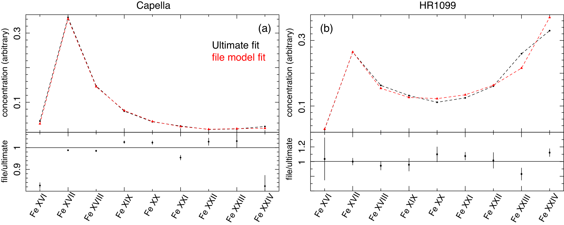
As shown in Figure 1, the total ion concentration with model 1 can be determined by combining the ion concentration of each component weighed by the emission measure derived from the fit. To compare the model concentration with the observed one, we re-fit the spectra by allowing the model component of each IOI free to vary. This can be done by the SPEX file model, which reads a spectral model from an ASCII file. The emission of IOIs are now modeled by multiple file models, each contains the line plus continuum of one IOI from all the spectral components. The remaining non-IOI spectra are converted to another file model. The astrophysical and instrumental corrections are applied to all the file models. This would allow us to determine the absolute ion concentration directly from the observation which does not depend on the temperatures of the CIE components. Through a fit of the Capella and HR 1099 spectra, we determine the normalizations of the file components, and thus the deviations on ion concentrations from the values with model 1. For the Fe IOIs shown in Figure 1, the measured deviation is less than 20% at worst, with an average value of 8% for Capella and 10% for HR 1099. Similar values can be obtained with the other IOIs. The current estimate is also in good agreement with the uncertainties obtained in Hitomi Collaboration et al. (2018) for the Perseus cluster.

It should be noted that the measured deviation might not come fully from the ion concentration uncertainty alone. For several IOIs, the thermal emission is dominated by the strong emission lines. A possible systematic bias in the emissivities of the strongest transitions could therefore cause potential deviation in the measured concentration of the relevant IOI. In addition, the emissivities of radiative and dielectronic recombination and innershell ionization transitions are determined by the concentration of the neighbour ions. The changes of their emissivities due to the changes in relative ion concentration are not accounted in the current approach. As both effects would introduce extra deviations to the IOI concentration measurement, we consider the deviation shown in Figure 1 as a crude approximation to the actual atomic uncertainty in ion concentration.

2.2.2 Uncertainties on line intensities

Next we address the uncertainties on line emissivities. First, we define the lines of interest (LOIs), which are set as a collection of the strongest X-ray lines of the IOIs. For each Fe ion, we pick up the top 200 lines, and exclude those in the UV range. For the other elements, we do the same but for top 50 lines. These numbers of lines are determined empirically to make sure that all the lines visible in the three test spectra are included. The LOIs are selected at the average temperatures (weighted by the emission measure of each component) of the objects. A full list of the LOIs selected based above criteria is provided in Table LABEL:tab:longtable.

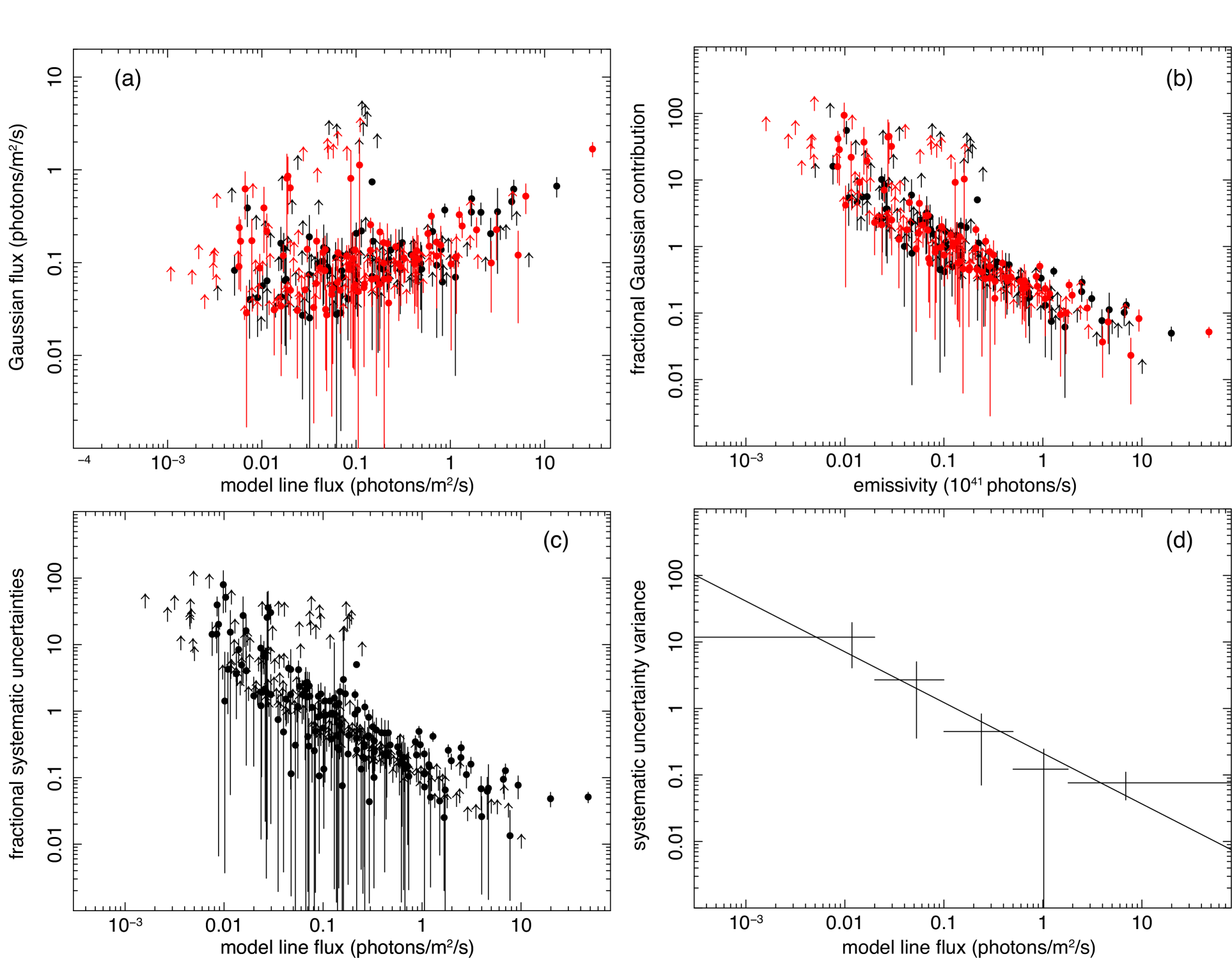
To determine the emissivity uncertainty of each LOI, we add for each LOI an emission line with a Gaussian shape to our ultimate spectral model. The line energy is fixed to the energy of the target LOI, the width is determined as described below, and the normalization is directly determined from a spectral fit and represents the difference in flux between the prediction by the ultimate model and the measured spectrum. A part of the LOIs cannot be resolved as they are blended within the instrumental resolution. In such cases, we use one Gaussian component for one line blend, and set the Gaussian central wavelength to the average of the unresolved LOIs weighted by the emissivities. The line widths of the resolved Gaussian components are fixed to the thermal plus turbulent broadening of the target LOIs, while for the blended lines, the widths are set free. We have tested to let all the line widths free, and found that the best-fit line fluxes vary typically by $\leq 20$%. As shown later in Figure 4, the variation of the line width has a negligible effect on our conclusion.

The Gaussian components are further corrected for the known astrophysical and instrumental effects, including the ionized/neutral absorption, the systematic line shift, and the residual calibration errors on the effective area as well as on the line spread function as described in § 2.1. Parameters of these models are fixed to the values determined from the original fits with model 1. We define model 2 as a co-addition of model 1, which is now converted to a file model as to take into account the uncertainties on ion concentration, and the set of Gaussian components. The normalizations of the Gaussian components are the parameters of main interest, the positive normalizations account for lines where the model underestimates the data, while the negative normalizations (or absorption-like components) represent the opposite.

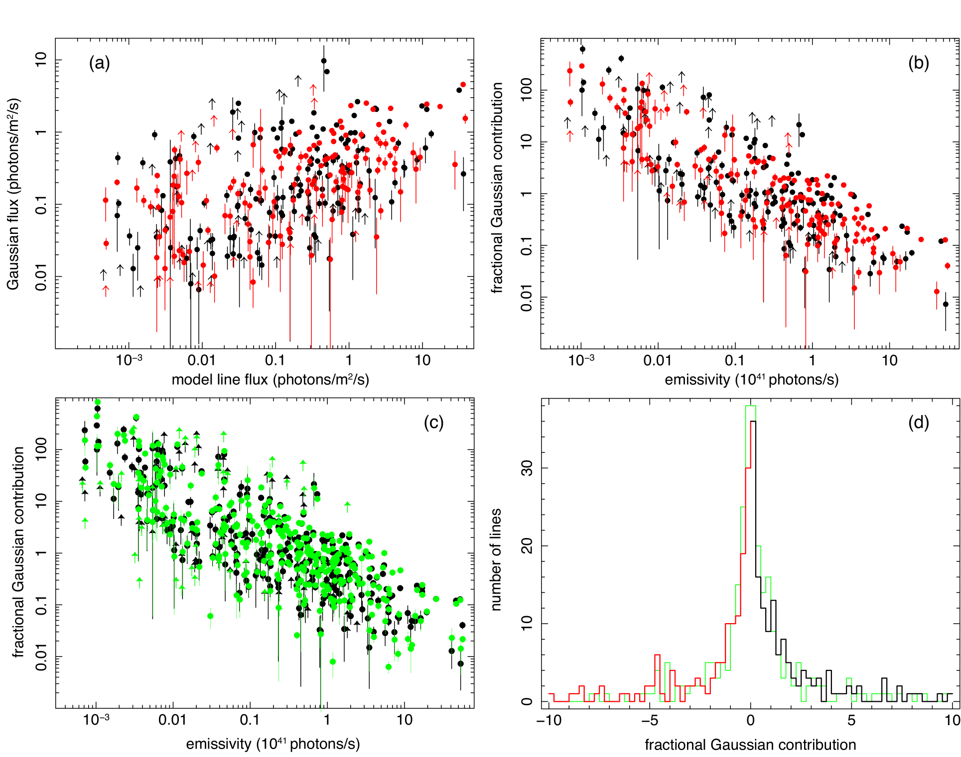
Although the additional Gaussian components with free widths for the blends result in a large number of free parameters with model 2 (656 for Capella and HR 1099, and 186 for the Perseus cluster), most of the Gaussian components are well constrained, or have well defined upper bounds on fluxes (Figs. 2, 5, and 6). This is because that, at first, all the Gaussian components, including those for the blends, are well resolved in the test spectra and fit independently; and secondly, model 2 contains nearly zero degrees of freedom on the astrophysical model (e.g., emission measure, temperature, and abundances) by converting it to a set of file models.

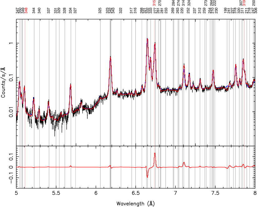
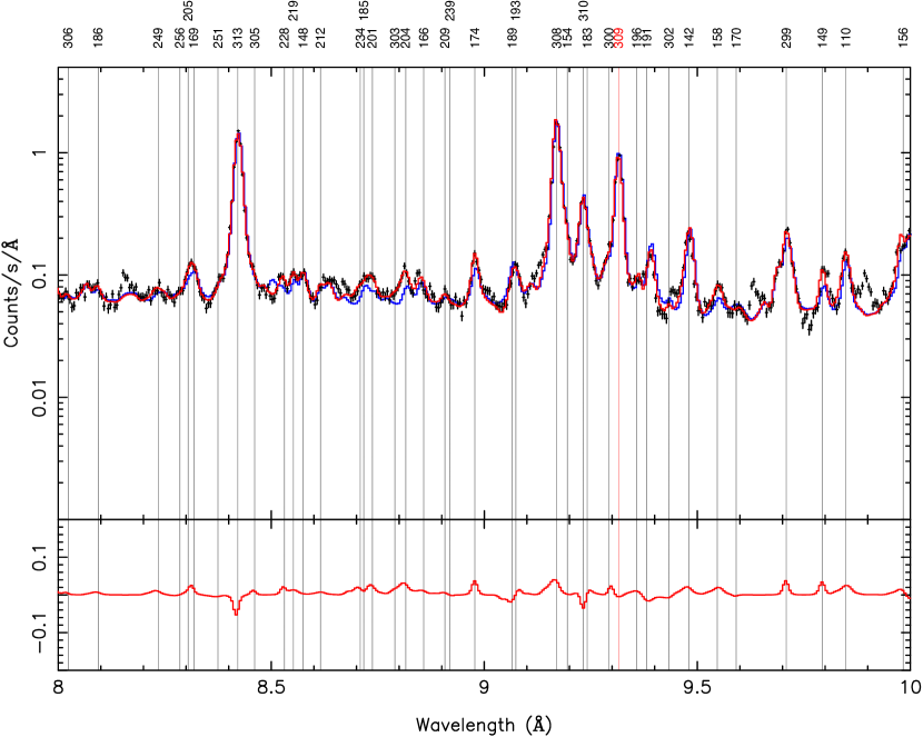
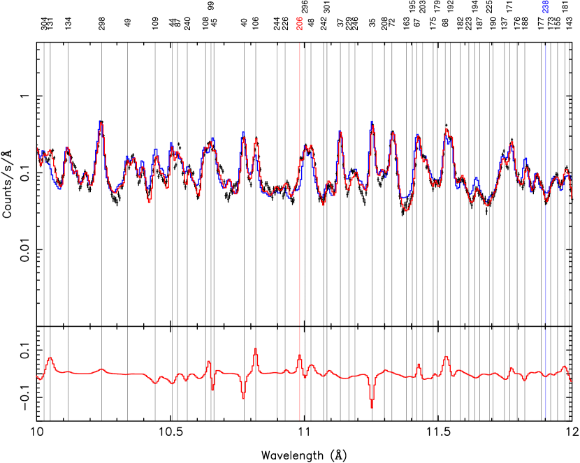
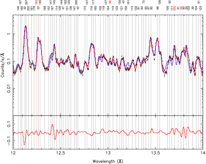
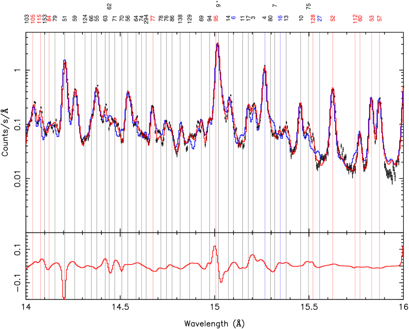
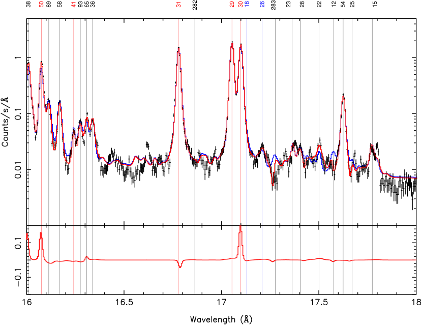
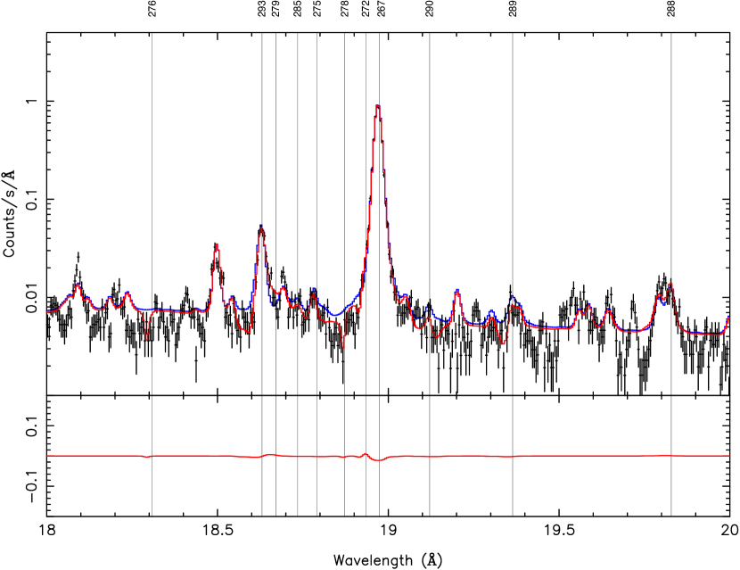
Figures 17 and 18 plot a comparison of model 1 and model 2 for the Capella HETG spectrum. It reveals significant discrepancies between model 1 and the observed spectrum in a range of positions, most of those likely originate from issues in the atomic data that calculate the line fluxes. Most of the discrepancies appear to be solved with model 2, which compensates for the mismatches by fitting the extra Gaussian components. As seen in the lower panels of the figures, these Gaussian components contribute up to $\sim 20$% of the corresponding line fluxes, and vary strongly, in both positive and negative ranges, among different LOIs or line blends.

For Capella, the C-stat has been improved from 40281.2 with model 1 to 13520.3 with model 2, for an ideal expectation of 6555. As shown in Figures 17 and 18, model 2 has fixed the issues in the previous fits of Fe XVIII lines in $14-16$ Å, Fe XIX-XXI lines in $12-14$ Å, Fe XXII-XXIII lines around 11.8 Å, and Fe XVII-XIX lines in $10-11$ Å. Although model 2 has accurately reproduced most of the lines in the spectrum, the overall fit is still formally unacceptable. The remaining discrepancies should be understood as residual errors in instrument calibration, combined with the minor inadequacies of the atomic data (in particular on wavelengths, see Paper II). Yet there are a few observed weak lines, such as those at 9.64 Å, 9.89 Å, 10.68 Å, 10.86 Å, 16.62 Å, and 17.80 Å, still missing in the present modeling. Ignoring the spectral bins containing the missing lines could further reduce the C-stat to 10343.

As stated earlier, the present work is based on a systematic comparison between model 1 and model 2 on the known atomic transitions. We will demonstrate later (§ 2.2.3) that the remaining issues in the fit with model 2, such as the missing weak transitions at a few places, have a negligible influence on the systematic comparison. It would therefore be valid to consider the Gaussian components, which quantify the difference between model 1 and model 2, as an approximation to the total uncertainties in the SPEX line modeling with respect to the actual data. In panel (a) of Figure 2, the model 2 minus model 1 differential flux (i.e., flux of each Gaussian component added to model 2) is plotted against the model 1 line flux for each LOI. It shows that the differential fluxes are positively correlated with model line fluxes; a flat distribution assuming all Gaussian lines have a common flux can be excluded at $>5\sigma$. This implies that the observed differential fluxes cannot be fully explained by the systematic uncertainties due to the instrumental calibration, which do not depend on the fluxes of the observed lines.

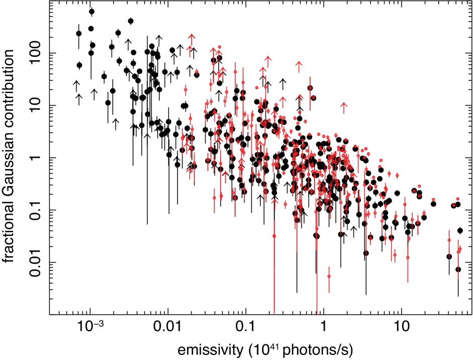
By dividing the Gaussian fluxes by the total fluxes of the corresponding lines, we further obtain the fractional uncertainties. As shown in panel (b) of Figure 2, the uncertainties show anti-correlation with the line emissivities; for the strong transitions with emissivities $\geq 5\times 10^{41}$ photons s^-1, the fractional uncertainties are found to be around 10%, while for the weak lines $\sim 10^{39}$ photons s^-1, the uncertainties increase to unity or even larger. In addition, panel (c) of Figure 2 shows that the variation of Gaussian line widths has a nearly negligible effect on the observed uncertainty-emissivity relation.

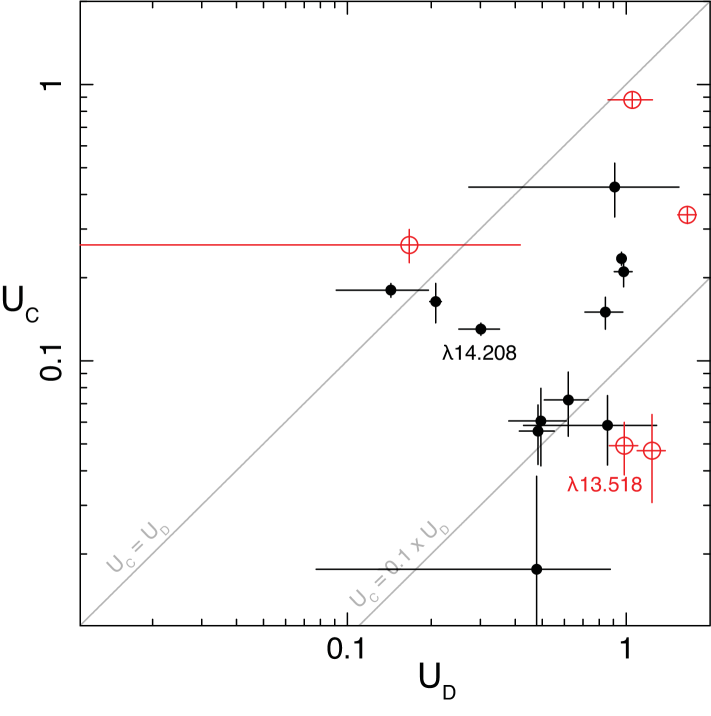
In Figure 3 we compare the fractional uncertainties for several Fe XVIII and Fe XIX transitions reported in Desai et al. (2005) and those obtained in the our work. It can be found that the present uncertainties are systematically smaller than those from Desai et al. (2005), for instance, the discrepancies between the model and data on Fe XVIII resonance line at 14.208 Å and Fe XIX line at 13.518 Å have been reduced from 30% and 98% (Desai et al. 2005) to the present values of 13% and 5%. This means that the current modeling of the Capella spectrum, though still far from ideal, has already been improved significantly from the those used in Desai et al. (2005) on in particular the atomic database.

The Gaussian fluxes shown in Figure 2 can be treated as a combination of statistical and systematic uncertainties. By subtracting the statistical uncertainties in quadrature from the total values, we estimate the systematic uncertainties from the line modeling (Fig. 4 left panel). It can be seen that the contributions of statistical uncertainties are minor for most of LOIs, thanks to the high quality of the Capella spectrum. To describe the uncertainty-emissivity relation, we divide the emissivity range into a number of emissivity bins, and assume for each bin that the distribution of systematic uncertainty follows a Gaussian function with zero mean value. As seen in panel (d) of Figure 2, the total uncertainty does show a distribution that can be described by a combination of multiple Gaussian components peaked at zero with different variances. The derived variances of the systematic uncertainties are plotted in the right panel of Figure 4 as a function of emissivity. It turns out that the systematic uncertainty-emissivity relation could be approximated by a simple power-law function,

$$\sigma=a\times\left(\frac{I}{10^{41}}\right)^{b},$$ (1)

where $\sigma$ is the variance of systematic uncertainties, $I$ is line emissivity in unit of photons s^-1, $a$ and $b$ are the free parameters. The line emissivities are calculated for a standard CIE model with proto-solar abundances (Lodders et al. 2009) and a fixed emission measure of $10^{64}$ m^-3. As shown in Table 1, the parameters $a$ and $b$ are found to be 1.020 and -0.563 for Capella. The subsets with positive and negative Gaussian normalizations (black and red data points in Fig. 2) can be described by the same power-law function as the combined set.

Table 1: Fit parameters and errors of the observed uncertainty-emissivity relations with Eq. 1.

	$T_{\rm peak}$ (keV)	a	b
Capella	0.5	1.020 (0.150)	-0.563 (0.067)
HR 1099	1.5	0.212 (0.084)	-0.762 (0.217)
Perseus	4.0	0.103 (0.183)	-0.946 (0.511)
All	$-$	0.332 (0.058)	-0.623 (0.104)

In addition to Capella, we have applied the same exercise to the HR 1099 (Chandra HETG) and the Perseus cluster (Hitomi) spectra. The differential fluxes obtained in model 2, the systematic uncertainties, and the variances are plotted against the line emissivity in Figs. 5 and 6. These two objects have higher peak temperatures (1.5 keV for HR 1099 and 4 keV for Perseus) than Capella (0.5 keV). One should also note that the Hitomi spectrum of the Perseus cluster contains only the K-shell lines above 2 keV, whereas the Capella spectrum is dominated by the Fe-L shell lines. Despite of the differences, the two objects exhibit similar trends in the systematic uncertainty-emissivity diagram as Capella (Figure. 7). This reinforces the general picture that the strong emission lines are consistently much better modeled than the weak ones. This picture seems to hold for both the L-shell and the K-shell lines, though the latter is vastly overnumbered by the former in the current test. As shown in Table 1, the power-law fits to the HR 1099 and Perseus variances reveal marginal difference from Capella: the best-fit relations of HR 1099 and Perseus cluster appear to be slightly steeper than Capella, implying for smaller systematic uncertainties in the modeling of strong lines for the objects with higher average temperatures. A similar hint can be inferred from the right panel of Figure 7, where we compare the systematic uncertainties for the common lines that appear in both Capella and HR 1099 spectra. For the same transition, the fractional error obtained with Capella (low temperature) is systematically higher than that with HR 1099 (high temperature), indicating that the uncertainty on line flux is likely a temperature-dependent variable rather than a constant. Verifying this possible dependence would require a follow-up study with a systematic spectroscopic sample to cover both the L-shell and K-shell emissions.

2.2.3 Influence of the weak transitions

As described earlier, a few weak emission features in the Capella spectrum are not fully accounted for by the present model, indicating that the atomic data for the minor transitions are not yet complete. As the missing line issue could also occur to the blends with other lines, it thus becomes vital to evaluate the effect of weak lines on the results obtained so far.

In Figure 8 we compare the original fractional uncertainties of Capella with the uncertainties obtained with a modified model, in which the Gaussian components of the known transitions of emissivity below $1.5\times 10^{39}$ photons per second are removed in the fit. Ignoring these components means many weak lines are wrongly modeled, even so, it seems that they do not alter much the uncertainties of the strong transitions. The uncertainty-emissivity relation of the strong transitions remains largely intact in the comparison; parameters $a$ and $b$ from Eq. 1 change by 6% and 1% from the original values in Table 1. Therefore, our results obtained so far should be robust against the present limitation in atomic data on weak transitions.

2.3 Dependence on various factors

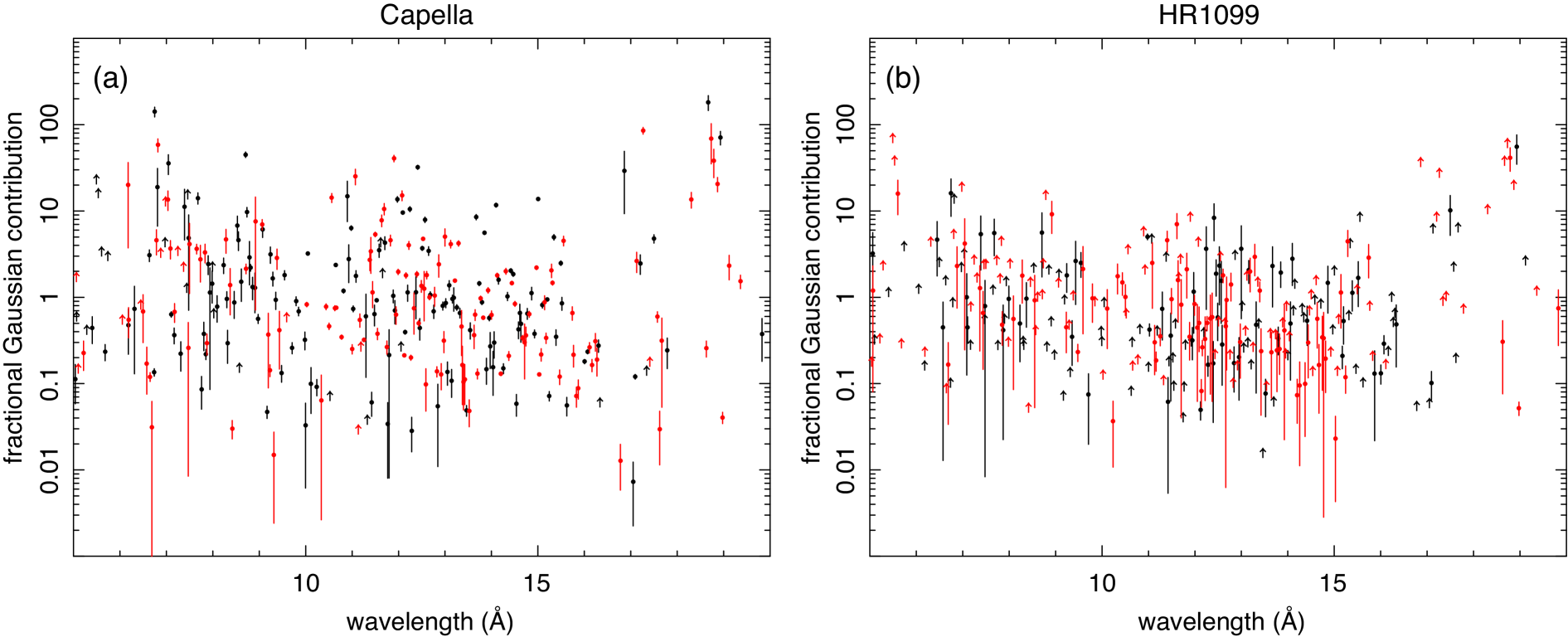
In order to understand the origin of the observed uncertainty-emissivity relation, here we examine its possible dependence on several variables including the line wavelength, ion species, and dominant line formation processes. As shown in Figure 9, the total uncertainty on the line flux is plotted as a function of wavelength for each individual line in the Capella and HR 1099 spectra. We find no clear evidence for dependence on line positions; the relative errors seem to be equally distributed across the energy band, except for a small group of lines at long wavelengths ($\sim 19$ Å) where the uncertainties are larger than the average. Figure 18 shows that the present spectral model of Capella does not fully reproduce the observed continuum between $17-19$ Å, which might partially explain the large line uncertainties. However, this potential bias only affects a small subset of the lines, which is minor to the uncertainty-emissivity relation obtained with the entire set. Therefore, we conclude that the systematic uncertainties on line fluxes are independent on the line positions.

Next we divide the entire line sample into groups by the ion species. As shown in Figure 10, the Fe ion groups can be found at different positions in the line emissivity range, which is primarily determined by the ion concentration of the source. In general, the distribution of each individual group appears to follow the combined distribution described by the analytic form (Eq. 1). There might be a small number of minor biases in individual groups, such as Fe XIX, which shows a flatter uncertainty-emissivity relation than the average one for HR 1099, though for Capella it agrees well with the average relation. We also find good agreement between the Fe group and the non-Fe group. Therefore, it is likely that the same power-law dependence of spectral uncertainties on line emissivity can be applied to most of the ions in the present collisional plasma model.

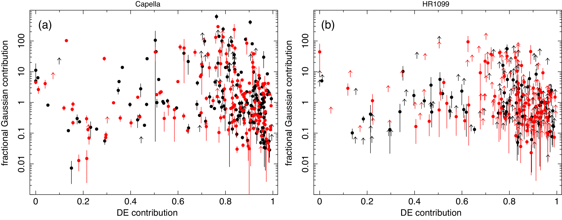
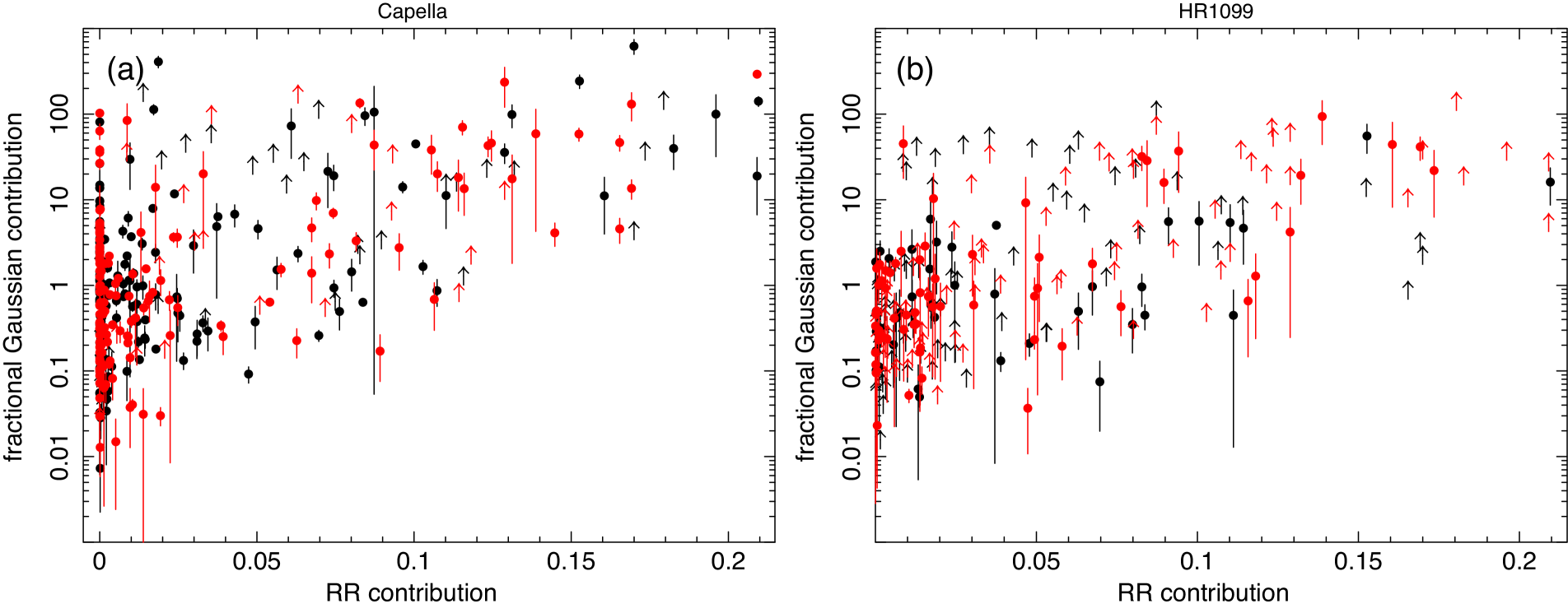
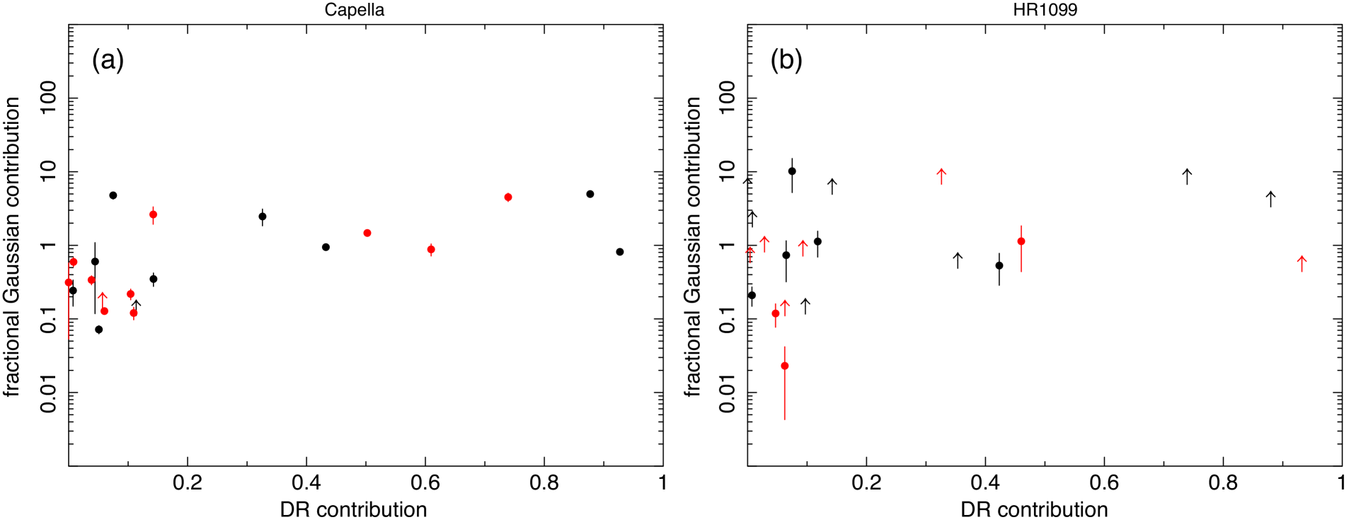
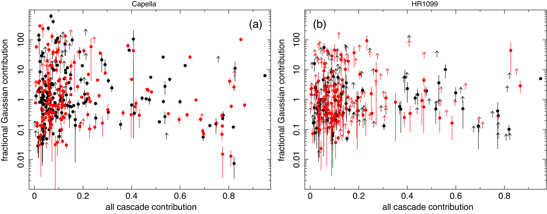
Finally let us consider the effect of line formation processes. We calculate the contributions to the upper levels of the LOIs by various processes: collisional excitation, radiative recombination, dielectronic recombination, and the cascades from these processes to lower levels. The fractional contributions calculated for Capella are shown in Table LABEL:tab:longtable. As seen in Figure 11, there is no obvious correlation between the line uncertainties and the collisional excitation contribution for Capella and HR 1099. The same is found for the dielectronic recombination (though with much less data; Fig. 13) and the cascade contribution (Fig. 14). As for the radiative recombination (Fig. 12), we can see a hint for a weak positive correlation against the line uncertainty, however, the current significance is rather low, as the data points with large radiative recombination contribution are very sparse. Overall, it suggests that the observed uncertainty-emissivity relation is unlikely to be fully ascribed to one specific line formation process, but rather caused by the atomic uncertainties in the theoretical calculations of multiple relevant processes.

It should be noted that some line formation processes might be further affected by the physical properties of stellar coronae, for example, the finite density and electric or magnetic fields. As discussed in, e.g., Mewe (1999), the dielectronic recombination rate might be suppressed in high density plasma due to the ionization of doubly excited states, while it can be enhanced by a factor of $5-10$ by the influence of external electric fields. These two effects might explain some individual scatters observed in the Capella and HR 1099 spectra, however, they alone cannot explain the uncertainty-emissivity relation due to the scarcity of strong dielectronic recombination lines in the observed spectra (Fig. 13).

Figure 15: (a) G ratio of O VII as a function of temperature with associated uncertainties calculated for low density plasma. (b) R ratio of O VII as a function of electron density with an electron temperature of $10^{6}$ K. The black data with errors show our results, the red curves and shaded areas represent the peaks and the associated errors reported in Loch et al. (2013). The blue and green curves show the results with AtomDB (Smith et al. 2001; Foster et al. 2012).

Figure 16: A part of the simulated XRISM (left) and Athena (right) spectra for a 1 keV CIE model, with the associated uncertainties shown in thin grey curves. The original model is plotted in red.

As a summary, we discover a relation between the systematic uncertainties and the line emissivities based on the high-quality spectra of Capella, HR 1099, and the Perseus cluster. This power-law like relation holds for spectra with different instruments, objects with different temperature, and lines at different positions and from different ions. It cannot be explained by errors in individual line formation process. The observed relation might describe a universal feature of the state-of-the-art atomic database.

3 Applications

In this paper, we present a study of systematic uncertainties in modeling of collisional sources using observational data. A key application of the results (e.g., Eq. 1) would be to provide quick and reliable estimate of atomic uncertainties for a range of relevant observables, including in particular the line ratios (e.g., He-like triplet), emission measure, temperature, and abundances. These parameters are the key science outcomes from the present and future X-ray spectroscopic instruments, their intrinsic uncertainties are vital, albeit so far often missing, to our understanding of the astrophysical sources.

3.1 He$\alpha$ triplet line ratios

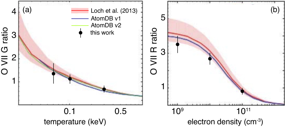
At first we apply our phenomenological relation (Eq. 1) to evaluate the systematics on the He-like line ratios. In Figure 15, we show the uncertainties associated with the O VII He$\alpha$ triplet line ratios compared with the previous results. For a low-density plasma, the error on the G ratio is found to be $\sim 35$% at 0.05 keV and $\sim 5$% at 0.5 keV. The uncertainty on the R ratio with a temperature of $10^{6}$ K is $\sim 15$% at an electron density of $1\times 10^{9}$ cm^-3 and diminishes with increasing density. These values in general agree with the uncertainties for the same transitions reported in Loch et al. (2013), though the two are derived with very different approaches. The uncertainties of Loch et al. (2013) were obtained from a Monte-Carlo calculation with fundamental atomic constants, while our values come directly from observations.

We attempted to do the same comparison with the published results on the lines in ultraviolet (Yu et al. 2018; Del Zanna et al. 2019), however, the present quality of atomic database in SPEX for these ultraviolet lines is still insufficient to provide useful constraint on their emissivities.

3.2 Atomic uncertainties for XRISM and Athena

Next we apply the obtained line uncertainties to realistic simulations with complicated spectral models, and estimate the induced errors on the primary model parameters, e.g., plasma temperature, emission measure, and elemental abundances. We simulate a set of spectral model by varying all the model line intensities using the observed uncertainty-emissivity relation (Eq. 1 and Table 1). For simplicity we use the average relation with $a=0.332$ and $b=-0.623$. To avoid negative or absorption features, the lower boundary of new line emissivities is set to zero. The upper limit on the fractional uncertainty is set to 100 for the weakest transitions, which is approximately the maximal uncertainty observed in the Capella spectrum (Fig. 2). We test our method on the collisional ionization equilibrium spectrum for a set of temperature grids from $0.5-2.0$ keV (Table 2), which is about the temperature range of Capella and HR 1099 where the Fe-L lines dominate the spectrum. We intend to limit our exercise to relatively low temperatures as the obtained uncertainty-emissivity relation is primarily determined by the Fe L-shell lines from the observed spectra.

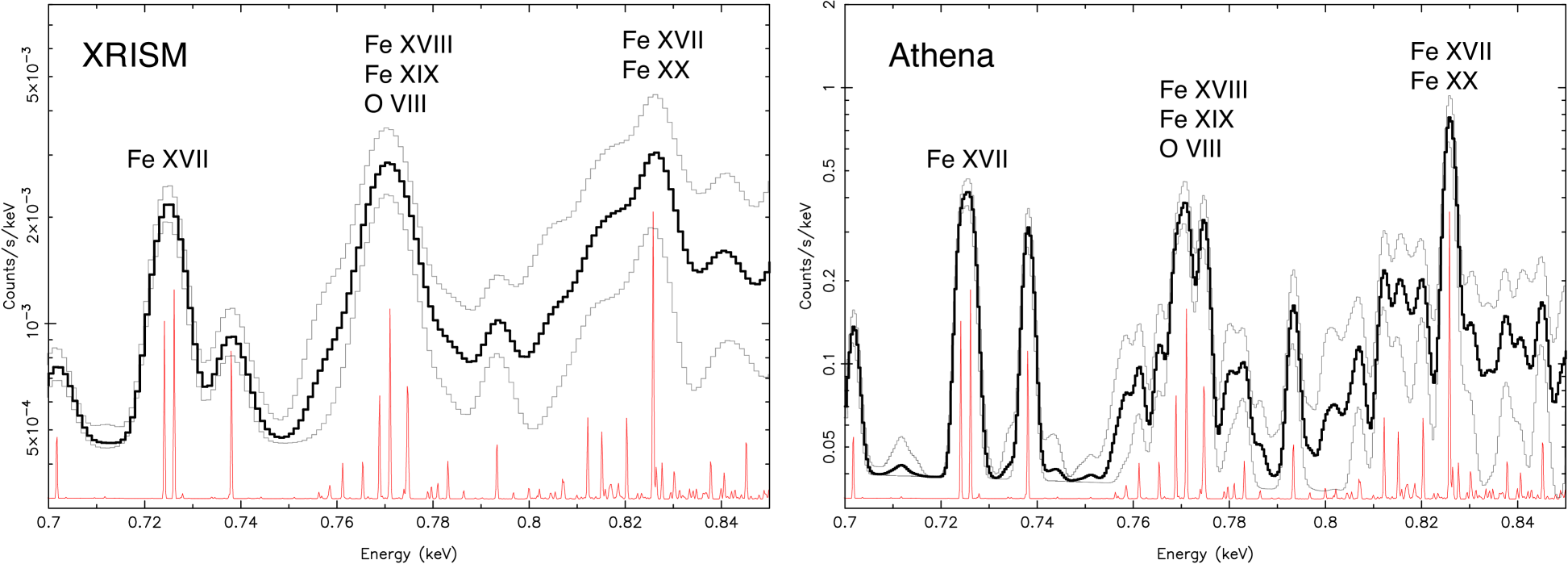
The simulated models are folded with the instrumental responses of XRISM Resolve and Athena X-ray Integral Field Unit (X-IFU). XRISM (due to launch in the early 2020s) and Athena (early 2030s) are two future X-ray observatories exploring the hot and energetic baryons in the Universe. These two missions will enable very well-resolved X-ray spectroscopy of various X-ray sources and will push the atomic modeling to its limit. In Figure 16 we illustrate a part of the spectrum, as well as the associated systematic uncertainty, of a turbulence-free 1 keV CIE model. We run the simulation 1000 times for each temperature grid and instrument, fit the randomized data with the original spectral model, and summarize in Table 2 the obtained standard deviations of the primary model parameters: emission measure, temperature, and abundances. For the abundances, we show the atomic uncertainties on Fe as well as several representative elements in the Fe-L region (O, Ne, Mg, and Ni). For the latter, the uncertainties originate from the errors on their own emission as well as on the blended neighbor Fe-L lines.

Table 2: Fractional systematic uncertainties on model parameters based on the simulation described in § 3.

kT	$\sigma_{\rm EM}$	$\sigma_{\rm kT}$	$\sigma_{\rm O}$	$\sigma_{\rm Ne}$	$\sigma_{\rm Fe}$	$\sigma_{\rm Mg}$	$\sigma_{\rm Ni}$
(keV)	XRISM
0.5	0.038	0.011	0.047	0.058	0.044	0.078	0.076
0.75	0.063	0.007	0.067	0.081	0.072	0.066	0.092
1.0	0.066	0.007	0.059	0.097	0.065	0.065	0.130
1.25	0.071	0.012	0.072	0.100	0.067	0.081	0.167
1.5	0.060	0.021	0.060	0.098	0.067	0.093	0.133
1.75	0.045	0.023	0.054	0.097	0.057	0.104	0.171
2.0	0.032	0.022	0.061	0.097	0.050	0.113	0.200
	Athena
0.5	0.033	0.011	0.029	0.047	0.043	0.067	0.050
0.75	0.039	0.007	0.040	0.059	0.039	0.048	0.056
1.0	0.044	0.005	0.048	0.072	0.035	0.053	0.091
1.25	0.051	0.008	0.065	0.077	0.038	0.071	0.112
1.5	0.052	0.019	0.080	0.087	0.053	0.092	0.128
1.75	0.041	0.023	0.078	0.091	0.053	0.103	0.153
2.0	0.031	0.022	0.070	0.092	0.049	0.111	0.175

As shown in Table 2, the uncertainties on line flux have propagated into $\sim 3-7$% errors on the emission measure (hence $2-4$% on gas density), $\sim 1-2$% on temperature, $\sim 4-7$% on O and Fe abundances, $\sim 6-10$% on Ne and Mg abundances, and $\sim 8-20$% on Ni abundance, for a XRISM-like spectrum. Some of these parameters are better constrained with Athena X-IFU, as X-IFU has a significantly better spectral resolution that helps to de-blend the lines in a crowded complex. The atomic uncertainties are further found to be temperature-dependent: the fractional temperature error increases by a factor of three from 1 keV to 2 keV, while the abundance errors show peaks around $1.25-1.5$ keV. The different behaviors of temperature and abundance errors show that they might originate from different sets of lines. Note that the obtained systematic uncertainties likely represent a lower limit, as (1) the continuum uncertainties, and the errors on the ionization balance calculation, are not yet included; and (2) in the present simulation the discrepancies on the line intensities are assumed to be fully random, which might not hold in reality.

4 Conclusion

We present an observational constraint that could be used to calculate the systematic uncertainties in spectral model of sources in collisional ionization equilibrium. Our method is based on statistical properties of the discrepancies between model line fluxes and observed values. The uncertainties are found to be about 10% for the strong emission lines, and significantly increase towards low fluxes. The observed uncertainty-emissivity relation can be approximated by an analytic form, which holds for lines with different wavelengths, ion species, and formation processes. Applying the observed uncertainties to the simulated XRISM and Athena spectra yields $4-20$% systematic errors on the elemental abundances measured from these spectra. In the future this work will be extended to the other spectral components (continuum and absorption features), and to astrophysical sources in photo-ionization and non-equilibrium ionization status. It should be emphasized that our approach based on observational data can provide absolute uncertainties of the target atomic constants, however, it cannot be used to illustrate the underlying correlations between the uncertainties of different transitions. Ideally, it will require fundamental theoretical calculations, benchmarked by the observational results, to derive a full picture of the atomic uncertainties.

The atomic uncertainties estimated using the new approach have been implemented in the aerror command of the SPEX code.

Appendix A Modeling details of the Capella and HR 1099 spectra

In Figures 17 and 18, we plot the Chandra HETG data fit with a plasma model and a file plus Gaussian line model (see details in § 2). We also show the ratios between the two models. For each line of interest, we list its position, flux, uncertainty, and line formation properties in Table LABEL:tab:longtable.

Figure 17: Stacked Chandra grating spectrum of Capella in $5.0-14.0$ Å (wavelength region divided by panels) fit with model 1 (ultimate model from paper II, blue) and model 2 (file model plus multiple Gaussian components, red). The relative discrepancies between model 1 and model 2 are shown in the lower panel. The selected lines of interest are marked with thin vertical lines. The numbers on the top are the associated line IDs (see Table LABEL:tab:longtable for details), the colors of the numbers indicate the dominant line formation process: black $-$ direct excitation; red $-$ radiative cascade; blue $-$ dielectronic recombination.

Figure 18: Same as Fig 17 but for $14-20$ Å.

Table 3: List of lines of interest

Ion	ID	Wavelength	EX	CEX	RR	CRR	DR	CDR	$I_{\rm Capella}$	$U_{\rm Capella}$	$I_{\rm HR1099}$	$U_{\rm HR1099}$
		($\AA$)							(ph m-2 s-1)		(ph m-2 s-1)
Fe XVI	1	40.1517	0.543	0.008	0.041	0.016	0.000	0.385	0.8458	0.0448	0.2479	0.1462
Fe XVI	2	39.8258	0.608	0.002	0.045	0.018	0.000	0.319	0.4057	0.1374	0.1163	0.4795
Fe XVI	3	15.2008	0.000	0.000	0.000	0.000	0.934	0.066	0.4529	0.9431	0.0616	0.5325
Fe XVI	4	15.2442	0.365	0.002	0.000	0.000	0.607	0.025	0.7161	0.0719	0.0962	0.1186
Fe XVI	3	15.2109	0.965	0.002	0.000	0.000	0.021	0.012	1.2664	0.9431	0.1756	0.5325
Fe XVI	3	15.2140	0.000	0.000	0.000	0.000	0.973	0.027	0.3508	0.9431	0.0456	0.5325
Fe XVI	5	36.7478	0.633	0.007	0.073	0.030	0.000	0.248	0.3032	21.4497	0.0741	12.7918
Fe XVI	4	15.2597	0.000	0.000	0.000	0.000	0.935	0.064	0.2516	0.0719	0.0329	0.1186
Fe XVI	6	15.0960	0.182	0.001	0.000	0.000	0.760	0.056	0.3394	0.8149	0.0452	0.2251
Fe XVI	7	15.3150	0.000	0.000	0.000	0.000	0.957	0.043	0.2498	1.4674	0.0335	0.2118
Fe XVI	6	15.0794	0.000	0.000	0.000	0.000	0.990	0.010	0.3070	0.8149	0.0457	0.2251
Fe XVI	6	15.0752	0.000	0.000	0.000	0.000	0.997	0.003	0.3107	0.8149	0.0463	0.2251
Fe XVI	8	35.1134	0.000	0.007	0.100	0.021	0.000	0.860	0.3103	2.1108	0.0709	11.3896
Fe XVI	9	15.0260	0.000	0.000	0.000	0.000	0.995	0.005	0.3035	0.1278	0.0454	0.0230
Fe XVI	6	15.0916	0.000	0.000	0.000	0.000	0.991	0.009	0.2497	0.8149	0.0371	0.2251
Fe XVI	9	15.0472	0.000	0.000	0.000	0.000	0.997	0.003	0.2931	0.1278	0.0446	0.0230
Fe XVI	9	15.0309	0.000	0.000	0.000	0.000	0.999	0.001	0.2940	0.1278	0.0448	0.0230
Fe XVI	5	36.8018	0.662	0.022	0.071	0.021	0.000	0.216	0.1502	21.4497	0.0365	12.7918
Fe XVI	1	40.2348	0.000	0.026	0.082	0.025	0.000	0.861	0.1891	0.0448	0.0622	0.1462
Fe XVI	9	15.0471	0.000	0.000	0.000	0.000	0.999	0.001	0.2363	0.1278	0.0360	0.0230

Table 3: continued.

1. Full data table can be found via the link to the machine-readable version.

2. ID: line ID (see Figs. 17 and 18)
   

3. EX/CEX/RR/CRR/DR/CDR: contributions of upper level population from direct excitation, excitation followed by cascades, radiative recombination, radiative recombination followed by cascades, dielectronic recombination, dielectronic recombination followed by cascades
   

4. $I_{\rm Capella}$, $I_{\rm HR\leavevmode\nobreak\ 1099}$: line fluxes from the best-fit models (model 1)
   

5. $U_{\rm Capella}$, $U_{\rm HR\leavevmode\nobreak\ 1099}$: fractional systematic uncertainties of the lines from the Gaussian fits (model 2)