Understanding quantum black holes from quantum reduced loop gravity

Abstract

We systematically study the top-down model of loop quantum black holes (LQBHs), recently derived by Alesci, Bahrami and Pranzetti (ABP). Starting from the full theory of loop quantum gravity, ABP constructed a model with respect to coherent states peaked around spherically symmetric geometry, in which both holonomy and inverse volume corrections are taken into account, and shown that the classical singularity used to appear inside the Schwarzschild black hole is replaced by a regular transition surface. To understand the structure of the model, we first derive several well-known LQBH solutions by taking proper limits. These include the Böhmer-Vandersloot and Ashtekar-Olmedo-Singh models, which were all obtained by the so-called bottom-up polymerizations within the framework of the minisuperspace quantizations. Then, we study the ABP model, and find that the inverse volume corrections become important only when the radius of the two-sphere is of the Planck size. For macroscopic black holes, the minimal radius obtained at the transition surface is always much larger than the Planck scale, and hence these corrections are always sub-leading. The transition surface divides the whole spacetime into two regions, and in one of them the spacetime is asymptotically Schwarzschild-like, while in the other region, the asymptotical behavior sensitively depends on the ratio of two spin numbers involved in the model, and can be divided into three different classes. In one class, the spacetime in the 2-planes orthogonal to the two spheres is asymptotically flat, and in the second one it is not even conformally flat, while in the third one it can be asymptotically conformally flat by properly choosing the free parameters of the model. In the latter, it is asymptotically de Sitter. However, in any of these three classes, sharply in contrast to the models obtained by the bottom-up approach, the spacetime is already geodesically complete, and no additional extensions are needed in both sides of the transition surface. In particular, identical multiple black hole and white hole structures do not exist.

I Introduction

The resolution of General Relativity (GR) singularities is a well established result in Loop Quantum Gravity (LQG) [1], and is ultimately due to the presence of a minimum area implied by the quantum nature of the gravitational field. The studies of the cosmological singularity carried out in the last decades represent the first applications of LQG to cosmology [2, 3] in a well established research area now called Loop Quantum Cosmology (LQC) [4], which is already at the stage of predicting observable consequences [5, 6, 7]. LQC is built on first performing a classical symmetry reduction and then importing from the full theory a quantum structure adapted to the reduced system, namely the polymer quantization [8].

The LQC success in identifying the resolution of the Big Bang singularity naturally shifted the effort to study black hole interiors [9, 10] with LQC techniques: classical symmetry reduction and polymer quantization of the resulting minisuperspace. However, in both contexts the quantization procedure leaves several ambiguities: LQC needs to import from the full theory the area gap, and part of the quantum degrees of freedom are lost once the classical symmetry reduction is performed. In fact, in LQG the quantum states of the gravitational field are spinnetwork states labeled by spins (SU(2) quantum numbers, the eigenvalues of the geometrical operators, such as the area and volume operators, etc.) and graphs on 3-dimensional manifolds with vertices locating the quanta space and realizing arbitrary quantum spaces. On the other hand, in LQC dealing with classically homogenous models the Hilbert space can’t accommodate graphs and the polymer quantization employed is not sensible to the SU(2) representations. These ambiguities have been fixed [11] in the cosmological setting with the evolution from the $\mu_{0}$ to the $\bar{\mu}$ scheme [12], while for black holes, although there are many proposals [13, 14, 17, 18, 16, 15, 19, 20, 21, 22, 23, 24, 25, 27, 26, 28, 29, 32, 33, 34, 30, 31, 37, 46, 35, 36, 38, 40, 41, 42, 43, 44, 45, 39, 49, 50, 47, 48, 49, 51, 52, 53, 54, 55], their LQC treatment is still evolving. In both schemes the origin of the ambiguities is rooted in the fact that there is no fixed prescription to obtain the LQC Hilbert space from the LQG one and the fundamental property of LQG, namely the existence of space quanta, can only be imported. Now if the introduction of a minimum volume as external input is enough to solve the singularity, details of the evolution deeply depend on the amount of structure imported ad hoc from the full theory.

Recently, a new technique (Quantum Reduced Loop Gravity - QRLG) aimed to disentangle those ambiguities was proposed by Alesci, Bahrami and Pranzetti (ABP), the so-called top-down approach [56]. QRLG is based on the tentative of reverting the reduction-quantization process to implement a quantum symmetry reduction. Performing gauge fixing to adapt the full quantization to the symmetry compatible coordinates, QRLG allows to study the homogeneous spacetimes as coherent states of the full theory retaining all the quantum degrees of freedom of LQG. In this sense, QRLG doesn’t need an external area gap or an ad-hoc Hilbert space, because it just uses the full LQG Hilbert space. QRLG program has been successfully applied to cosmology [57] and a direct link to LQC has been unveiled [58]. However, the inclusion of new degrees of freedom also opens the possibility for new scenarios as the replacement of the big bounce scenario [59] with the emergent bouncing one [60]. The application of QRLG to the interior of a black hole [61, 62] has been recently performed and showed a completely new possibility. The black hole singularity is replaced by a bounce followed by an expanding Universe that could be asymptotically de Sitter [63].

In this paper, we shall study the ABP model in detail and confirm several major conclusions obtained in [62, 63], and meanwhile clarify some silent points. In particular, the article is organized as follows. In Sec. II, we provide a brief review of the ABP model [61, 62, 63], by paying particular attention to its semi-classical limit conditions, which are essential in order to understand the physical implications of the model. In Sec. III, we first consider its classical limit, whereby the physical interpretation of quantities of the ABP model become clear, and then obtain the Böhmer-Vandersloot (BV) [13] and Ashtekar-Olmedo-Singh (AOS) models [30, 31] by taking proper limits and replacements. In doing so, we look for the possible relation among these models. Although formally we can obtain all these models, they all fall to the case where the semi-classical limit conditions of the ABP model are not satisfied. As a result, these models cannot be embedded properly into the ABP model. However, we do find that such derivation is helpful in understanding the structure of the ABP model. In Sec. IV, we study the ABP model without the inverse volume corrections in detail, by first showing that such corrections become important only when the curvature becomes the order of the Planck scale. The subsequent detailed analysis shows that the minimal radius of the two-sphere obtained at the transition surface is always much larger than the Planck scale for macroscopic black holes. As a result, the inverse volume corrections should be always sub-leading for such black holes. In Sec. V, we confirm this by focusing only on the cases with $\gamma=0.274$ obtained by the considerations of black hole entropy [64], and $j_{x}$ and $j$ given by Eq.(2.21) below, obtained by demanding that the spatial manifold triangulation remain consistent on both sides of the black hole horizons [63]. Our main results are summarized in Sec. VI, while in Appendix A, we provide some properties of the Struve functions.

In this paper, we shall use $\ell_{p},m_{p},\tau_{p}$ to denote, respectively, the Planck length, mass and time. In all the numerical plots, we shall use them as the units. For example, when plotting a figure with $m=1$ we always mean $m/m_{p}=1$, and so on.

II Effective Hamiltonian of Internal spherical Black Hole Spacetimes

Spherically symmetric spacetimes inside black holes can be written in the form

$$ds^{2}=-N(\tau)^{2}d\tau^{2}+\Lambda(\tau)^{2}dx^{2}+R(\tau)^{2}d\Omega^{2},$$ (2.1)

where $N(\tau)$ is the lapse function and $d\Omega^{2}\equiv d\theta^{2}+\sin^{2}\theta d\phi^{2}$. Clearly, the above metric is invariant under the following transformations

$$\tau=\xi(\tau^{\prime}),\quad x=a_{0}x^{\prime}+b_{0},$$ (2.2)

where $\xi(\tau^{\prime})$ is an arbitrary function of $\tau^{\prime}$ and $a_{0}$ and $b_{0}$ are arbitrary constants.

II.1 Classical Spherical Spacetimes and Canonical Variables

It should be noted that, instead of using the canonic variables ($\Lambda,R$) and their momentum conjugates ($P_{\Lambda},P_{R}$), one often uses ($p_{b},b,p_{c},c$) [30], which can be obtained by comparing the gravitational connection $A^{i}_{a}\tau_{i}dx^{a}$ and the spatial triads $E_{i}^{a}\tau^{i}\partial_{a}$, given in [30, 63], and yield

$$p_{c} = R^{2},\quad p_{b}=L_{0}R\Lambda,\quad b=-\frac{\gamma G}{R}P_{\Lambda},$$

$$c = -\frac{\gamma GL_{0}}{R}\left(P_{R}-\frac{\Lambda P_{\Lambda}}{R}\right),$$ (2.3)

where $L_{0}$ is a constant, and related to ${\cal{L}}_{0}$ introduced in [63] by $L_{0}=2{\cal{L}}_{0}$. Note that in writing down the above expressions we assumed $p_{c}>0$. With the choice of the lapse function [30, 31]

$$N_{cl}=\gamma b^{-1}{\text{sgn}}(p_{c})\left|p_{c}\right|^{1/2}=-\frac{R^{2}}{GP_{\Lambda}},$$ (2.4)

we find that the metric (2.1) takes the form

$$ds^{2}=-\frac{\gamma^{2}p_{c}(T)}{b^{2}(T)}dT^{2}+\frac{p_{b}^{2}(T)}{L_{0}^{2}p_{c}(T)}dx^{2}+p_{c}(T)d\Omega^{2},$$ (2.5)

where

$$T\equiv\frac{\tau}{2Gm}+\log(2Gm).$$ (2.6)

Then, the corresponding classical Hamiltonian is given by

$$H_{cl}[N_{cl}] \equiv N_{cl}\mathcal{H}_{c}$$ (2.7)

$$= -\frac{1}{2G\gamma}\left(2c\;p_{c}+\left(b+\frac{\gamma^{2}}{b}\right)p_{b}\right)$$

$$= \frac{L_{0}R^{2}}{GP_{\Lambda}}\Bigg{(}\frac{GP_{\Lambda}P_{R}}{R}-\frac{GP_{\Lambda}^{2}\Lambda}{2R^{2}}+\frac{\Lambda}{2G}\Bigg{)}.$$

II.2 Quantum Black Holes in QRLG

Within the framework of QRLG, starting from a partial gauge fixing of the full LQG Hilbert space, ABP [61, 62, 63] studied the interior of a Schwarzschild black hole, and derived an effective Hamiltonian by including the inverse volume and coherent state sub-leading corrections, which differs crucially from the ones introduced previously in the minisuperspace models. In particular, by fixing the quantum parameters associated with the structure of coherent states through geometrical considerations, the authors found that the post-bounce interior geometry sensitively depends on the value of the Barbero-Immirzi parameter $\gamma$, and that the value $\gamma\simeq 0.274$, deduced from the SU(2) black hole entropy calculations in LQG [65, 64], gives rise to an asymptotically de Sitter geometry in the interior region .

Introducing the following parameters

$$A \equiv 2{\ell_{p}}^{2}\left(\frac{{\ell_{p}}^{2}\gamma^{2}}{\beta^{2}}-\frac{4\gamma^{2}}{\delta_{x}}+\frac{4(3-\nu)\gamma^{2}}{\delta}\right),$$

$$B \equiv {\ell_{p}}^{2}\left(\frac{{\ell_{p}}^{2}\gamma^{2}}{\beta^{2}}-\frac{8\gamma^{2}}{\delta_{x}}+\frac{8(3\nu-1)\gamma^{2}}{\delta}\right),$$

$$C \equiv 2{\ell_{p}}^{2}\left(\frac{{\ell_{p}}^{2}\gamma^{2}}{\alpha^{2}}+\frac{12\gamma^{2}}{\delta_{x}}-\frac{4(1+\nu)\gamma^{2}}{\delta}\right),$$ (2.8)

and the functions

$$X \equiv \alpha\gamma G\left(\frac{P_{\Lambda}}{R^{2}}\right),\quad Y\equiv\beta\gamma G\left(\frac{P_{R}}{R\Lambda}-\frac{P_{\Lambda}}{R^{2}}\right),$$

$$Z \equiv 8\gamma^{2}\cos\left(\frac{\alpha}{R}\right)\sin^{2}\left(\frac{\alpha}{2R}\right),$$ (2.9)

we find that the effective Hamiltonian of the ABP model can be cast in the form

$$\mathcal{H}_{int}^{IV+CS}=-\frac{\mathcal{L}_{0}R^{2}\Lambda}{2\alpha^{2}\gamma^{2}G}\mathcal{C}(\tau),$$ (2.10)

where

$$\mathcal{C}(\tau)\equiv\frac{\alpha}{\beta}\sin[Y]\Bigg{\{}\left(1+\frac{A}{R^{2}}\right)\pi h_{0}[X]$$

$$~{}~{}~{}~{}~{}~{}~{}~{}~{}~{}~{}~{}~{}~{}~{}~{}~{}~{}~{}~{}~{}~{}~{}+2\left(1+\frac{B}{R^{2}}\right)\sin[X]\Bigg{\}}$$

$$~{}~{}~{}~{}~{}~{}~{}~{}~{}~{}+Z+\left(1+\frac{C}{R^{2}}\right)\pi\sin[X]h_{0}[X],$$ (2.11)

and $\mathcal{L}_{0}$ denotes the length of the fiducial cell with $x\in\left[-\mathcal{L}_{0},\mathcal{L}_{0}\right]$, and ${\ell_{p}}$ is the Planck length with ${\ell_{p}}\equiv\sqrt{\hbar G/c^{3}}$, while $G$ and $c$ are the Newton’s constant and the speed of light, respectively. The super indices “IV” and “CS” stand for, respectively, the inverse volume and coherent state, while the dimensionless parameters $\delta,\;\delta_{x}$ and $\nu$ are the spread parameters, characterizing the coherent state corrections. The terms proportional to the constants $A,B$ and $C$ characterize the inverse volume corrections and are subdominant [63]. The function $h_{0}[X]$ denotes the zeroth-order Struve function and its series expansion reads [67]

$$h_{0}[z]=\frac{2}{\pi}\left(z-\frac{z^{3}}{1^{2}\cdot 3^{2}}+\frac{z^{5}}{1^{2}\cdot 3^{2}\cdot 5^{2}}-...\right).$$ (2.12)

In Fig. 1, we plot out the Struve function $h_{0}$ together with $h_{-1}$, as the latter will appear in the dynamical equations. In general, the $\nu$-th order Struve functions are defined by Eq.(A.1) in Appendix A, in which some of their properties are also given. For more details, we refer readers to [67].

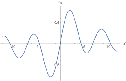
(a)

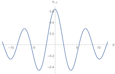
(b)

Figure 1: The Struve functions $h_{0}[X]$ and $h_{-1}[X]$.

In terms of the spin numbers $j$ and $j_{x}$, the parameters $\alpha$ and $\beta$ are given by

$$\alpha\equiv 2\pi\sqrt{\gamma j_{x}}\;{\ell_{p}},\quad\beta\equiv 4\sqrt{\frac{8\pi\gamma}{j_{x}}}\;j\;{\ell_{p}},$$ (2.13)

where $j_{x}$ denotes the averaged spin number of all plaquettes that tessellate the 2-sphere $S^{2}$ spanned by $(\theta,\phi$), while $j$ is the averaged spin number associated with the links dual to the plaquettes in both ($\theta,x$) and ($\phi,x$) planes. It must be noted that this effective Hamiltonian is valid only in the semi-classical limits [63]

$$j,\;j_{x}\gg 1.$$ (2.14)

To understand further the geometrical meaning of $j$ and $j_{x}$, we introduce the coordinate lengths along $x,\;\theta,\;\phi$ directions by $\epsilon_{x},\;\epsilon_{\theta},\;\epsilon_{\phi}$, respectively. Due to the spherical symmetry, we have $\epsilon_{\theta}=\epsilon_{\phi}\equiv\epsilon$. Then, we introduce two new quantities ${\cal{N}}$ and ${\cal{N}}_{x}$, in terms of which $\epsilon$ and $\epsilon_{x}$ can be written as

$$\epsilon\equiv\frac{2\pi}{{\cal{N}}},\quad\epsilon_{x}\equiv\frac{{\cal{L}}_{0}}{{\cal{N}}_{x}},$$ (2.15)

where ${\cal{N}}^{2}/2$ is the total number of the plaquettes on $S^{2}$, and ${\cal{N}}_{x}$ denotes the total number of plaquettes in the $x$ direction for a given fiducial length ${\cal{L}}_{0}$. The effective Hamiltonian (2.10) was obtained under the assumption

$${\cal{N}},\;{\cal{N}}_{x}\gg 1\;\;\;\text{or}\;\;\;\epsilon,\;\epsilon_{x}\ll 1.$$ (2.16)

To find the relations between (${\cal{N}},\;{\cal{N}}_{x}$) and ($j,j_{x}$), we can calculate the area of a given $S^{2}$ and the volume of a given spatial three-surface spanned by $x,\theta,\phi$, which are given, respectively, by

$$A(R) = 4\pi R^{2}=8\pi\gamma\ell_{p}^{2}\sum_{p\in S^{2}}\tilde{j}^{p}_{x}\simeq 8\pi\gamma\ell_{p}^{2}\left(\frac{{\cal{N}}^{2}}{2}j_{x}\right),~{}~{}~{}~{}~{}~{}~{}$$ (2.17)

$$V(\Sigma) = 8\pi{\cal{L}}_{0}\Lambda R^{2}\simeq 4\left(8\pi\gamma\ell_{p}^{2}\right)^{3/2}j\sqrt{j_{x}}{\cal{N}}_{x}{\cal{N}}^{2},$$ (2.18)

where $\tilde{j}^{p}_{x}$ is the spin number associated with the link dual to the given plaquettes $p$ on $S^{2}$. In the limit ${\cal{N}}\gg 1$, the sum of $\tilde{j}^{p}_{x}$ in Eq.(2.17) was approximated by the average spin $j_{x}$ of a single cell times the total number of the plaquettes in $S^{2}$. In the last step of Eq.(2.18), the average spin number $j$ is associated with the links dual to the plaquettes in both ($x,\theta$)- and ($x,\phi$)-planes. Therefore, we find

$${\cal{N}}=\frac{R}{\sqrt{\gamma\ell_{p}^{2}}}\left(\frac{1}{\sqrt{j_{x}}}\right),\quad{\cal{N}}_{x}=\frac{{\cal{L}}_{0}\Lambda}{4\sqrt{8\pi\gamma\ell_{p}^{2}}}\left(\frac{\sqrt{j_{x}}}{j}\right).~{}~{}~{}~{}~{}~{}~{}~{}~{}~{}$$ (2.19)

Inserting Eq.(2.19) into Eq.(2.15), we obtain

$$\epsilon=\frac{\alpha}{R},\quad\epsilon_{x}=\frac{\beta}{\Lambda},$$ (2.20)

where $\alpha$ and $\beta$ are defined by Eq.(2.13).

It should be noted that the understanding of the geometrical meaning of ${\cal{N}},{\cal{N}}_{x},j$ and $j_{x}$ is important for our following discussions, especially when we consider some specific models within the framework of QRLG. As to be seen below, both of the semi-classical limit conditions (2.14) and (2.16) must be fulfilled, in order to have the effective Hamiltonian (2.10) valid. These also provide the keys for us to understand the semi-classical structures of black holes in the framework of LQG.

We further note that, by demanding that the spatial manifold triangulation remain consistent on both sides of the black hole horizons, ABP found [63]

$$j=\gamma j_{x},$$ (2.21)

for which we have

$$\eta\equiv\frac{\alpha}{\beta}=\frac{\sqrt{2\pi}}{8\gamma},$$ (2.22)

as can be seen from Eq.(2.13). Then, in the effective Hamiltonian (2.10) five new parameters

$$(\gamma,j;\nu,\delta,\delta_{x})\;\;\;\text{or}\;\;\;(\gamma,\alpha;\nu,\delta,\delta_{x}),$$

are present in addition to $G,c,\hbar$, where ($\nu,\delta,\delta_{x}$) are related to the inverse volume corrections. One of the purposes of this paper is to understand their effects on the local and global properties of the spacetimes.

It should be noted that the two spin numbers $j$ and $j_{x}$ used in this paper, which are consistent with those used in [63], are different from the ones ($\hat{j},\hat{j}_{0}$) introduced in [62] . In particular, we have

$$\hat{j}=\sqrt{8\pi}\;j,\quad\hat{j}_{0}=\frac{\pi}{2}j_{x}.$$ (2.23)

To write down the corresponding dynamic equations for the effective Hamiltonian (2.10), using the gauge freedom (2.2), ABP chose the lapse function $N(\tau)$ as

$$N(\tau)=-\frac{2\alpha\gamma}{mGW},$$ (2.24)

where $m$ is a mass parameter, and $W$ is defined as

$$W = \pi h_{0}[X]+2\sin[X].$$ (2.25)

Taking $\hbar\rightarrow 0$, it reduces to

$$N_{c}\equiv\;\lim_{\hbar\rightarrow 0}{N}=-\frac{R^{2}}{2mG^{2}P_{\Lambda}},$$ (2.26)

which corresponds to the classical limit, and $m$ represents the mass of the Schwarzschild black hole. Taking Eq.(2.6) into account, we find that

$$N_{c}^{2}d\tau^{2}=N_{cl}^{2}dT^{2},\quad N_{cl}=2GmN_{c},$$ (2.27)

where $N_{cl}$ and $N_{c}$ are given, respectively, by Eqs.(2.4) and (2.26).

Then, the smeared effective Hamiltonian of Eq.(2.10) with the choice of the lapse function (2.24) is given by

$$H_{int}^{IV+CS}[N] \equiv N(\tau)\mathcal{H}_{int}^{IV+CS}=\frac{\mathcal{L}_{0}R^{2}\Lambda}{\alpha\gamma mG^{2}W}{\cal{C}}(\tau).~{}~{}~{}~{}~{}~{}~{}$$ (2.28)

Hence, the corresponding dynamical equations can be cast in the form

$$-2Gm\frac{z}{\ell}R^{\prime} = \frac{R\cos[Y]}{W}{\cal{D}},$$ (2.29)

$$-2Gm\frac{z}{\ell}P_{\Lambda}^{\prime} = \frac{RP_{R}\cos[Y]}{\Lambda W}{\cal{D}},$$ (2.30)

$$-2Gm\frac{z}{\ell}\frac{\Lambda^{\prime}}{\Lambda} = -\frac{\cos[Y]}{W}{\cal{D}}+\frac{1}{W^{2}}\Bigg{\{}\pi h_{-1}[X]\Bigg{[}2\left(1+\frac{C}{R^{2}}\right)\sin^{2}[X]-Z\Bigg{]}+\cos[X]\Bigg{[}\left(1+\frac{C}{R^{2}}\right)\pi^{2}h_{0}^{2}[X]-2Z\Bigg{]}$$ (2.31)

$$+\frac{2\pi\alpha(A-B)}{\beta R^{2}}\sin[Y]\Big{(}\sin[X]h_{-1}[X]-\cos[X]h_{0}[X]\Big{)}\Bigg{\}},$$

$$-2Gm\frac{z}{\ell}P_{R}^{\prime} = \frac{RP_{R}-2\Lambda P_{\Lambda}}{RW}\cos[Y]{\cal{D}}+\frac{2\pi\Lambda P_{\Lambda}}{RW}\sin[X]h_{-1}[X]\left(1+\frac{C}{R^{2}}\right)$$ (2.32)

$$+\frac{2\pi\Lambda}{RW}h_{0}[X]\Bigg{\{}\left(\frac{C}{\alpha\gamma G}\right)\sin[X]+P_{\Lambda}\cos[X]\left(1+\frac{C}{R^{2}}\right)\Bigg{\}}$$

$$+\frac{2\Lambda\sin[Y]}{RW}\Bigg{\{}\frac{\alpha\pi}{\beta}P_{\Lambda}h_{-1}[X]\left(1+\frac{A}{R^{2}}\right)+\frac{A}{\beta\gamma G}\pi h_{0}[X]+\frac{2B}{\beta\gamma G}\sin[X]+\frac{2\alpha}{\beta}P_{\Lambda}\cos[X]\left(1+\frac{B}{R^{2}}\right)\Bigg{\}}$$

$$-\frac{4\gamma\Lambda}{GW}\Bigg{\{}\sin\left(\frac{\alpha}{R}\right)-\sin\left(\frac{2\alpha}{R}\right)\Bigg{\}},$$

where

$${\cal{D}}(X)\equiv\left(1+\frac{A}{R^{2}}\right)\pi h_{0}[X]+2\left(1+\frac{B}{R^{2}}\right)\sin[X],~{}~{}~{}~{}~{}~{}~{}~{}$$ (2.33)

and a prime denotes the ordinary derivative with respect to $z$, with $z\equiv\exp(-\tau/\ell)$, where $\ell$ is a constant and has the length dimension. The function $h_{-1}[X]\left(\equiv dh_{0}[X]/dX\right)$ denotes the Struve function of order $-1$. In Appendix A, we present some basic properties of these functions, and for other properties of them, we refer readers to [67].

III Some Known Loop Quantum Black Holes as Particular Limits of the ABP Model

To understand the quantum reduced loop black hole (QRLBH) spacetimes with both of the holonomy and inverse volume corrections, in this section let us first consider some limits of the parameters involved, and derive several well-known spacetimes. In doing so, we can gain a better understanding of the QRLBH spacetimes and their relation with other models.

III.1 Classical Limit

The classical limit is obtained by taking $\hbar\rightarrow 0$, that is, by setting $\ell_{p}=0$, which leads to

$$A=B=C=0,$$

$$\mathcal{D}\simeq W\simeq 4X,\quad Z\simeq\frac{2\gamma^{2}\alpha^{2}}{R^{2}}.$$ (3.1)

Then, Eqs.(2.29) - (2.32) reduce respectively to

$$-2Gm\frac{z}{\ell}R^{\prime} = R,$$ (3.2)

$$-2Gm\frac{z}{\ell}P_{\Lambda}^{\prime} = \frac{RP_{R}}{{\Lambda}},$$ (3.3)

$$-2Gm\frac{z}{\ell}\frac{\Lambda^{\prime}}{\Lambda} = -\frac{G^{2}P_{\Lambda}^{2}+R^{2}}{2G^{2}P_{\Lambda}^{2}},$$ (3.4)

$$-2Gm\frac{z}{\ell}P_{R}^{\prime} = 3P_{R}-\frac{2\Lambda P_{\Lambda}}{R}+\frac{\Lambda R}{G^{2}P_{\Lambda}},$$ (3.5)

while the effective Hamiltonian (2.10) reduces to (2.7) with $L_{0}=2{\cal{L}}_{0}$. Then, from the Hamiltonian constraint $\mathcal{H}_{c}=0$, we find the following two useful expressions

$$\frac{RP_{R}}{\Lambda} = \frac{G^{2}P_{\Lambda}^{2}-R^{2}}{2G^{2}P_{\Lambda}},$$ (3.6)

$$\frac{\Lambda P_{\Lambda}}{R} = 2P_{R}+\frac{R\Lambda}{G^{2}P_{\Lambda}}.$$ (3.7)

Inserting them into Eqs.(3.3) and (3.5), respectively, we obtain two new equations for $P_{\Lambda}^{\prime}$ and $P_{R}^{\prime}$, and together with the other two, they can be cast in the forms

$$-2Gm\frac{z}{\ell}R^{\prime} = R,$$ (3.8)

$$-2Gm\frac{z}{\ell}P_{\Lambda}^{\prime} = \frac{G^{2}P_{\Lambda}^{2}-R^{2}}{2G^{2}P_{\Lambda}},$$ (3.9)

$$-2Gm\frac{z}{\ell}\frac{\Lambda^{\prime}}{\Lambda} = -\frac{G^{2}P_{\Lambda}^{2}+R^{2}}{2G^{2}P_{\Lambda}^{2}},$$ (3.10)

$$-2Gm\frac{z}{\ell}P_{R}^{\prime} = -\frac{G^{2}P_{\Lambda}P_{R}+\Lambda R}{G^{2}P_{\Lambda}}.$$ (3.11)

Now, the above equations can be solved in sequence, that is, we first solve Eq.(3.8) to find $R(z)$, and then substituting it into Eq.(3.9), we can find $P_{\Lambda}(z)$. Once $R(z)$ and $P_{\Lambda}(z)$ are given, we can substitute them into Eq.(3.10) to find $\Lambda(z)$. Then, we can find $P_{R}(z)$ either by integrating Eq.(3.11) explicitly or by using the Hamiltonian constraint $\mathcal{H}_{c}=0$. In the first approach, we shall have four integration constants, but only three of them are independent, as the Hamiltonian constraint $\mathcal{H}_{c}=0$ must be satisfied, which will relate one of the four constants to the other three. Therefore, a simpler way is to solve $\mathcal{H}_{c}=0$ directly to find $P_{R}$, once $R,P_{\Lambda}$ and $\Lambda$ are found from Eqs.(3.8)-(3.10). However, to illustrate what we mentioned above, let us first integrate the above four equations directly to get

$$R = c_{0}e^{\frac{\tau}{2Gm}},$$ (3.12)

$$P_{\Lambda} = \mp\frac{\sqrt{c_{1}G^{2}e^{\frac{\tau}{2Gm}}-{c_{0}}^{2}e^{\frac{\tau}{Gm}}}}{G},$$

$$\Lambda = c_{2}e^{-\frac{\tau}{4Gm}}\sqrt{c_{1}G^{2}-c_{0}^{2}e^{\frac{\tau}{2Gm}}},$$ (3.13)

$$P_{R} = c_{3}e^{-\frac{\tau}{2Gm}}\pm\frac{c_{0}c_{2}}{G},$$ (3.14)

where $c_{n}$’s are the four integration constants. As noticed above, only three of them are independent. In fact, substituting the above expressions into the Hamiltonian constraint $\mathcal{H}_{c}=0$ we find that

$$c_{1}c_{2}G=\mp 2c_{0}c_{3}.$$ (3.15)

On the other hand, from Eq.(2.24), we find

$$N = -\frac{R^{2}}{2mG^{2}P_{\Lambda}}$$ (3.16)

$$= \pm\frac{c_{0}^{2}e^{\frac{\tau}{Gm}}}{2Gm\sqrt{c_{1}G^{2}e^{\frac{\tau}{2Gm}}-c_{0}^{2}e^{\frac{\tau}{Gm}}}}.$$

Thus, we finally obtain

$$ds_{c}^{2} = -N^{2}d\tau^{2}+\Lambda^{2}dx^{2}+R^{2}d\Omega^{2}$$

$$= -\frac{dR^{2}}{\frac{G^{2}c_{1}}{c_{0}R}-1}+c_{0}^{2}c_{2}^{2}\left(\frac{G^{2}c_{1}}{c_{0}R}-1\right)dx^{2}+R^{2}d\Omega^{2}.$$

Clearly, using the gauge residual (2.2), we can always absorb the factor $c_{0}^{2}c_{2}^{2}$ into $x$ by setting $a_{0}\equiv(c_{0}c_{2})^{-1}$. Then, the metric essentially depends only on one independent combination, $G^{2}c_{1}/c_{0}$, of the parameters, which is related to the mass of the black hole via the relation

$$m\equiv\frac{c_{1}G}{2c_{0}}.$$ (3.18)

It should be noted that the integration constants $c_{n}$’s can be also determined by the boundary conditions

$$R=2Gm,\quad\Lambda=0,\quad P_{\Lambda}=0,\;(\tau=0),$$ (3.19)

and the Hamiltonian constraint at the horizon $\tau=0$, which will be elaborated in more detail below, when we try to solve the field equations (2.29) - (2.32) numerically for the general case. In the current case, it can be shown that the above conditions together with the Hamiltonian constraint lead to

$$c_{0}=2Gm,\quad c_{1}=\frac{c_{0}^{2}}{G^{2}},\quad c_{2}=\frac{1}{c_{0}},\quad c_{3}=\mp\frac{1}{2G},$$ (3.20)

so the classical metric finally takes its standard form

$$ds_{c}^{2} = \left(1-\frac{2Gm}{R}\right)^{-1}dR^{2}-\left(1-\frac{2Gm}{R}\right)dx^{2}$$ (3.21)

$$+R^{2}d\Omega^{2}.~{}~{}~{}~{}$$

III.2 Böhmer-Vandersloot Limit

Following the so-called $\bar{\mu}$ scheme in LQC [12], Böhmer-Vandersloot (BV) [13] considered the case in which the physical area of the closed loop is equal to the minimum area gap predicted by LQG

$$\Delta=2\sqrt{3}\pi\gamma\ell^{2}_{\text{p}}.$$ (3.22)

For example, the holonomy loop in the ($x,\theta$)-plane leads to

$$A_{x\theta}=\delta_{b}\delta_{c}p_{b},$$ (3.23)

while the one in the ($\theta,\phi$)-plane leads to

$$A_{\theta\phi}=\delta_{b}^{2}p_{c},$$ (3.24)

where the new variable $b,\;c$ and their moment conjugates $p_{b},\;p_{c}$ are related to the ABP variables through Eq.(II.1), which can be written in the form

$$p_{b} = L_{0}\Lambda R,\quad b=-\alpha^{-1}RX,$$

$$p_{c} = R^{2},\quad c=-\beta^{-1}{L_{0}}\Lambda Y,$$ (3.25)

where $X$ and $Y$ are defined in Eq.(II.2). Then, setting

$$A_{x\theta}=\Delta=A_{\theta\phi},$$ (3.26)

will lead to

$$\delta_{b}=\sqrt{\frac{\Delta}{p_{c}}},\quad\delta_{c}=\frac{\sqrt{\Delta{p_{c}}}}{p_{b}}.$$ (3.27)

Making the replacements

$$b\rightarrow\frac{\sin(\delta_{b}b)}{\delta_{b}},\quad c\rightarrow\frac{\sin(\delta_{c}c)}{\delta_{c}},$$ (3.28)

in the classical lapse function $N_{\text{cl}}$ (2.4) and Hamiltonian $H_{\text{cl}}$ (2.7), we obtain

$$N_{\text{BV}} = \frac{\gamma\delta_{b}\sqrt{p_{c}}}{\sin(\delta_{b}b)},$$ (3.29)

$$H^{\text{eff}}_{\text{BV}}[N] = -\frac{1}{2\gamma G}\Bigg{[}2\frac{\sin(\delta_{c}c)}{\delta_{c}}p_{c}$$ (3.30)

$$+\left(\frac{\sin(\delta_{b}b)}{\delta_{b}}+\frac{\gamma^{2}\delta_{b}}{\sin(\delta_{b}b)}\right)p_{b}\Bigg{]}.$$

It is remarkable to note that the above effective Hamiltonian can be obtained from the ABP Hamiltonian without the inverse volume corrections presented in the last subsection. In fact, making the following approximation

$$h_{0}[X]\rightarrow\frac{2}{\pi}\sin[X],\quad\cos[\epsilon]\sin^{2}\left[\frac{\epsilon}{2}\right]\rightarrow\frac{\epsilon^{2}}{4},$$ (3.31)

where $\epsilon$ is defined in Eq.(2.20), we find that

$$A = B=C=0,$$

$$W \simeq 4\sin[X],\quad\mathcal{D}\simeq 4\sin[X],$$

$$\frac{\mathcal{D}}{W} \simeq 1,\quad Z\simeq 2\gamma^{2}\left(\frac{\alpha}{R}\right)^{2},$$

$$h_{-1} \simeq \frac{2}{\pi}\cos[X].$$ (3.32)

Then, substituting the above into the effective Hamiltonian (2.10), we shall obtain precisely the BV Hamiltonian (3.30) with

$$\delta_{b}=\frac{\alpha}{R}=\frac{\alpha}{\sqrt{p_{c}}},\quad\delta_{c}=\frac{\beta}{\Lambda L_{0}}=\frac{\beta\sqrt{p_{c}}}{p_{b}}.$$ (3.33)

Comparing them with those given by Eq.(3.27), we find that

$$\alpha^{\text{(BV)}}=\beta^{\text{(BV)}}=\sqrt{\Delta},$$ (3.34)

which immediately leads to

$$j^{\text{(BV)}} = \sqrt{\frac{3}{128\pi}}\simeq 0.0864\simeq 0.313j^{\text{(BV)}}_{x}>\gamma j^{\text{(BV)}}_{x},$$

$$j^{\text{(BV)}}_{x} = \frac{\sqrt{3}}{2\pi}\simeq 0.275.$$ (3.35)

Therefore, the BV Hamiltonian is precisely the limit of the effective ABP Hamiltonian, provided that:

• the inverse volume corrections vanish, $A=B=C=0$;

• the Struve functions $h_{0}[X]$ and $h_{-1}[X]$ are replaced respectively by $(2/\pi)\sin[X]$ and $(2/\pi)\cos[X]$; and

• the spin parameters $j_{x}$ and $j$ are chosen as those given by Eq.(III.2).

It is clear that the last condition is in sharp conflict with the semi-classical limit requirement of Eq.(2.14).

In addition, as $T\rightarrow-\infty$, BV found the following asymptotic behaviors

$$b \simeq \bar{b},\quad p_{b}\simeq\bar{p}_{b}e^{-\bar{\alpha}T},$$

$$c \simeq \bar{c}e^{-\bar{\alpha}T},\quad p_{c}\simeq\bar{p}_{c},$$ (3.36)

where $\bar{b},\bar{p}_{b},\bar{c},\bar{p}_{c}$ and $\bar{\alpha}>0$ are constants, given by [cf. Eqs.(64) - (69) in [13]]

$$2\sin(\bar{\delta}_{b}\bar{b})-\sin(\bar{\delta}_{b}\bar{b})^{2}=\frac{\Delta\gamma^{2}}{\bar{p}_{c}},$$ (3.37)

$$\bar{\alpha}=-\cos(\bar{\delta}_{b}\bar{b})+\cot(\bar{\delta}_{b}\bar{b}),$$ (3.38)

$$\sin(\bar{\delta}_{b}\bar{b})-\left(\bar{\delta}_{b}\bar{b}+\frac{\pi}{2}\right)\Big{[}\cos(\bar{\delta}_{b}\bar{b})-\cot(\bar{\delta}_{b}\bar{b})\Big{]}-2=0,$$

with

$$\bar{\delta}_{b}=\frac{\sqrt{\Delta}}{\sqrt{\bar{p}_{c}}},\quad\bar{\delta}_{c}=\frac{\sqrt{\Delta\;\bar{p}_{c}}}{\bar{p}_{b}},\quad\bar{\delta}_{c}\bar{c}=-\frac{\pi}{2}.$$ (3.40)

Then, from Eqs.(3.27) and (3.29) we find that asymptotically

$$N_{\text{BV}}\simeq\bar{N}\equiv\frac{\gamma\sqrt{\Delta}}{\sin(\bar{\delta}_{b}\bar{b})}.$$ (3.41)

Hence, the spacetime is asymptotically described by the metric

$$ds^{2} = -{N}_{\text{BV}}^{2}dT^{2}+\frac{p_{b}^{2}}{L_{0}^{2}p_{c}}dx^{2}+p_{c}d\Omega^{2}$$ (3.42)

$$\simeq \left(\frac{\bar{t}_{0}}{\bar{t}}\right)^{2}\left(-d\bar{t}^{2}+d\bar{x}^{2}\right)+\bar{p}_{c}d\Omega^{2},$$

where

$$d\bar{t}=e^{\bar{\alpha}T}dT,\quad\bar{x}=\frac{\bar{p}_{b}}{{\bar{N}}L_{0}\sqrt{\bar{p}_{c}}}x,\quad\bar{t}_{0}\equiv\frac{\bar{N}}{\bar{\alpha}}.$$ (3.43)

Loop quantum black holes do not satisfy the classical Einstein’s equations. However, in order to study the loop quantum gravitational effects (with respect to GR), we introduce the effective energy-momentum tensor $T^{\;\text{eff}}_{\mu\nu}$ by $T^{\;\text{eff}}_{\mu\nu}\equiv G_{\mu\nu}$ , which takes the form

$$T^{\;\text{eff}}_{\mu\nu} \simeq \rho u_{\mu}u_{\nu}+p_{\bar{x}}\bar{x}_{\mu}\bar{x}_{\nu}+p_{\bot}\left(\theta_{\mu}\theta_{\nu}+\phi_{\mu}\phi_{\nu}\right),~{}~{}~{}~{}$$ (3.44)

in the current case, where $u_{\mu}=(\bar{t}_{0}/\bar{t})\delta^{\bar{t}}_{\mu}$, $\bar{x}_{\mu}=(\bar{t}_{0}/\bar{t})\delta^{\bar{x}}_{\mu}$, $\theta_{\mu}=\sqrt{p_{c}}\delta^{\theta}_{\mu}$, $\phi_{\mu}=\sqrt{p_{c}}\sin\theta\delta^{\phi}_{\mu}$, and

$$\rho \simeq \frac{1}{\bar{p}_{c}},\;\;p_{\bar{x}}\simeq-\frac{1}{\bar{p}_{c}},\;\;p_{\bot}\simeq-\frac{1}{\bar{t}_{0}^{2}}.$$ (3.45)

From the above it is clear that the spacetime corresponds to a spacetime with a homogeneous and isotropic perfect fluid only when $\bar{t}_{0}=\sqrt{\bar{p}_{c}}$. When $\bar{t}_{0}\not=\sqrt{\bar{p}_{c}}$, the radial pressure is different from the tangential one, despite the fact that they are all constants. The latter (with $\bar{t}_{0}\not=\sqrt{\bar{p}_{c}}$) can be interpreted as the charged Nariai solution [68]. In addition, we also have

$${\cal{R}}\simeq 2\left(\frac{1}{\bar{p}_{c}}+\frac{1}{\bar{t}_{0}^{2}}\right),$$

$$R_{\mu\nu}R^{\mu\nu}\simeq 2\left(\frac{1}{\bar{p}_{c}^{2}}+\frac{1}{\bar{t}_{0}^{4}}\right),$$

$$R_{\mu\nu\alpha\beta}R^{\mu\nu\alpha\beta}\simeq 4\left(\frac{1}{\bar{p}_{c}^{2}}+\frac{1}{\bar{t}_{0}^{4}}\right),$$

$$C_{\mu\nu\alpha\beta}C^{\mu\nu\alpha\beta}\simeq\frac{4\left(\bar{p}_{c}+\bar{t}_{0}^{2}\right){}^{2}}{3\bar{t}_{0}^{4}\bar{p}_{c}^{2}}.$$ (3.46)

It is remarkable to note that, even when $\bar{t}_{0}=\sqrt{\bar{p}_{c}}$, the spacetime is still not conformally flat. So, it must not be the de Sitter space. In fact, as noticed by BV [13], it is the Nariai space [69, 70].

On the other hand, from Eqs.(3.37)-(III.2), BV found the following solutions

$$\bar{b}\simeq 0.156,\;\;\;\bar{p}_{c}\simeq 0.182\ell_{p}^{2},\;\;\;\bar{\alpha}\simeq 0.670,$$

$$\frac{\bar{c}}{\bar{p}_{b}}\simeq-2.290m_{p}^{2},\;\;\;\bar{N}\simeq 0.689\ell_{p},$$ (3.47)

from which we find that

$$\bar{t}_{0}=\frac{\bar{N}}{\bar{\alpha}}\approx 1.029\ell_{p}\not=\sqrt{\bar{p}_{c}}\left(\approx 0.427\ell_{p}\right).$$ (3.48)

Therefore, the solution is asymptotically approaching to the charged Nariai solution [68], instead of the Nariai solution [69].

It should be noted that in the above calculations, BV took $\gamma\approx 0.2375$ in the expression $\Delta=2\sqrt{3}\pi\gamma\ell_{p}^{2}$. Instead, if we take $\gamma\approx 0.274$ [63] we find

$$\bar{N}\approx 0.854\ell_{p},\quad\bar{p}_{c}\approx 0.279\ell_{p}^{2},\;(\gamma\approx 0.274),$$

$$\bar{t}_{0}\equiv\frac{\bar{N}}{\alpha}\approx 1.275\ell_{p}\not=\sqrt{\bar{p}_{c}}\left(\approx 0.529\ell_{p}\right),$$ (3.49)

that is, even in this case the spacetime is still not asymptotically Nariai, but the charged Nariai [68].

III.3 Ashtekar-Olmedo-Singh Limit

From the analysis of the BV limit, it becomes clear that from the general ABP model, the AOS limit [30, 31] can be obtained by the replacements

$$h_{0}[X]\rightarrow\frac{2}{\pi}\sin[X],\quad h_{-1}[x]\rightarrow\frac{2}{\pi}\cos[X],$$

$$\cos[\epsilon]\sin^{2}\left[\frac{\epsilon}{2}\right]\rightarrow\frac{\epsilon^{2}}{4},$$ (3.50)

so that

$$W \simeq 4\sin[X],\quad\mathcal{D}\simeq 4\sin[X],$$

$$\frac{\mathcal{D}}{W} \simeq 1,\quad Z\simeq 2\gamma^{2}\left(\frac{\alpha}{R}\right)^{2}.$$ (3.51)

In addition, we must also set

$$A=B=C=0,$$

$$\delta_{b},\;\delta_{c}={\text{Constant.}}$$ (3.52)

Then, the resultant lapse function and effective Hamiltonian will be precisely given by the same form as Eqs.(3.29) and (3.30) but with different $\delta_{b},\;\delta_{c}$. With the above in mind, AOS found the following solutions [31]

$$\sin\left(\delta_{c}c\right)=\frac{2a_{0}e^{2T}}{a^{2}_{0}+e^{4T}},$$

$$\cos\left(\delta_{b}b\right)=b_{0}\frac{b_{+}e^{b_{0}T}-b_{-}}{b_{+}e^{b_{0}T}+b_{-}},$$

$$p_{b}=-\frac{GmL_{0}e^{-b_{0}T}}{2b_{0}^{2}}\left(b_{+}e^{b_{0}T}+b_{-}\right){\cal{A}},$$

$$p_{c}=4(Gm)^{2}\left(a_{0}^{2}+e^{4T}\right)e^{-2T},$$ (3.53)

where $m$ is an integration constant, related to the mass parameter as noticed previously, and

$${\cal{A}} \equiv \Big{[}2\left(b_{0}^{2}+1\right)e^{b_{0}T}-b_{-}^{2}-b_{+}^{2}e^{2b_{0}T}\Big{]}^{1/2},$$

$$a_{0} \equiv \frac{\gamma\delta_{c}L_{0}}{8Gm},\quad b_{0}\equiv\left(1+\gamma^{2}\delta_{b}^{2}\right)^{1/2},$$

$$b_{\pm} \equiv b_{0}\pm 1,$$ (3.54)

with

$$\delta_{b}b\in\left(0,\pi\right),\quad\delta_{c}c\in\left(0,\pi\right),$$

$$p_{b}\leq 0,\quad p_{c}\geq 0,\quad-\infty<T<0.$$ (3.55)

In terms of $p_{b}$ and $p_{c}$, the metric takes the form

$$ds^{2}=-N_{\text{AOS}}^{2}dT^{2}+\frac{p_{b}^{2}}{|p_{c}|L_{0}^{2}}dx^{2}+|p_{c}|d\Omega^{2},$$ (3.56)

where

$$N_{\text{AOS}} = \frac{\gamma\delta_{b}\;\text{sgn}\left(p_{c}\right)\left|p_{c}\right|^{1/2}}{\sin\left(\delta_{b}b\right)}$$

$$= \frac{2Gm}{{\cal{A}}}e^{-T}\left(b_{+}e^{b_{0}T}+b_{-}\right)\left(a_{0}^{2}+e^{4T}\right)^{1/2}.$$

From Eq.(III.3), it can be seen that the transition surface is located at $\partial p_{c}\left({\cal{T}}\right)/\partial T=0$, which yields

$${\cal{T}}=\frac{1}{2}\ln\left(\frac{\gamma\delta_{c}L_{0}}{8Gm}\right)<0.$$ (3.58)

There exist two horizons, located respectively at

$$T_{\text{BH}}=0,\quad T_{\text{WH}}=-\frac{2}{b_{0}}\ln\left(\frac{b_{0}+1}{b_{0}-1}\right),$$ (3.59)

at which we have ${\cal{A}}(T)=0$, where $T=T_{\text{BH}}$ is the location of the black hole horizon, while $T=T_{\text{WH}}$ is the location of the white hole horizon. In the region ${\cal{T}}<T<0$, the 2-spheres are all trapped, while in the one $T_{\text{WH}}<T<{\cal{T}}$, they are all anti-trapped. Therefore, the region ${\cal{T}}<T<0$ behaves like the internal of a black hole, while the one $T_{\text{WH}}<T<{\cal{T}}$ behaves like the internal of a white hole.

The extension across the black hole horizon can be obtained by the following replacements [30, 31]

$$b\rightarrow ib,\quad p_{b}\rightarrow ip_{b},$$

$$c\rightarrow c,\quad p_{c}\rightarrow p_{c}.$$ (3.60)

Then, AOS found that the corresponding Penrose diagram consists of infinite diamonds along the vertical direction, alternating between black holes and white holes, but the spacetime singularity used appearing at $p_{c}=0$ now is replaced by a non-zero minimal surface with

$$p^{\text{min}}_{c}=p_{c}({\cal{T}})>0,$$ (3.61)

where ${\cal{T}}$ is given by Eq.(3.58).

To completely fix the values of $\delta_{b}$ and $\delta_{c}$, AOS required that on the transition surface ${\cal{T}}$, the physical areas of $A_{x\theta}$ and $A_{\theta\phi}$ be equal to the area gap $\Delta$ [30, 31]

$$2\pi\delta_{c}\delta_{b}\left|p_{b}({\cal{T}})\right|=\Delta,$$ (3.62)

$$4\pi\delta_{b}^{2}p_{c}({\cal{T}})=\Delta.$$ (3.63)

It is interesting to note that, substituting Eq.(3.33) into the above equations, we find that

$$2\pi\alpha\beta=\Delta,\quad 4\pi\alpha^{2}=\Delta,$$ (3.64)

which are all independent of $p_{b}$ and $p_{c}$ and given by

$$\alpha=\frac{1}{2}\beta=\sqrt{\frac{\Delta}{4\pi}}=\sqrt{2\sqrt{2}\;\gamma}\;\ell_{p}.$$ (3.65)

Comparing it with Eq.(2.13) we find that

$$j^{\text{(AOS)}} = \frac{1}{4\pi^{3/2}}<\frac{1}{2},\quad j^{\text{(AOS)}}_{x}=\frac{1}{\sqrt{2}\;\pi^{2}}<\frac{1}{2},$$

$${j}^{\text{(AOS)}} = \sqrt{\frac{\pi}{8}}\;{j^{\text{(AOS)}}_{x}}\simeq 0.6265{j^{\text{(AOS)}}_{x}}>\gamma{j^{\text{(AOS)}}_{x}},~{}~{}~{}~{}$$ (3.66)

from which we find that such given $j$ and $j_{x}$ do not satisfy the semi-classical limit conditions (2.14) either. Therefore, the AOS model cannot be realized in the framework of QRLG either, although it can be obtained formally by the approximations (III.3) and (III.3) from the ABP model.

IV Quantum Reduced Loop Black Holes without Inverse Volume Corrections

Setting the three constants $A,B$ and $C$ to zero, the effective Hamiltonian (2.10) reduces to the one given in [62], but with the replacement of the constants $\alpha$ and $\beta$ by

$$\alpha\equiv\sqrt{8\pi\gamma}\;\ell_{p}\;\sqrt{\hat{j}_{0}},\quad\beta=\frac{\sqrt{8\pi\gamma}\;\ell_{p}\;\hat{j}}{\sqrt{\hat{j}_{0}}},\;\;\;$$ (4.1)

where now $\hat{j}_{0}$ and $\hat{j}$ denote the quantum numbers associated respectively with the longitudinal and angular links of the coherent states, as mentioned in Section II. The relations between ($j,j_{x}$) and $(\hat{j},\hat{j}_{0}$) are given explicitly by Eq.(2.23). Without causing any confusion, in the rest of this section we shall drop the hats from $(\hat{j},\hat{j}_{0}$):

$$(\hat{j},\hat{j}_{0})\quad\rightarrow\quad(j,j_{0}),$$

unless some specific statements are given.

It is interesting to note that dropping the terms that are proportional to the constants $A,\;B$ and $C$ defined in Eq.(II.2) is physically equivalent to assuming that

$$\frac{A}{R^{2}},\;\frac{B}{R^{2}},\;\frac{C}{R^{2}}\ll 1,$$ (4.2)

as can be seen from the effective Hamiltonian given by Eq.(2.10). Before proceeding further, let us first pause here for a while and consider the above limits. In particular, from Eqs.(2.13) and (2.21), we find $\alpha\sim\beta\sim\sqrt{j}\ell_{p}$, where “$\sim$” means “being the same order”. On the other hand, introducing the spread parameters $\delta_{i}$ via the relations [63]

$$\delta_{r} = \frac{\pi^{2}\ell_{\scriptscriptstyle P}^{2}R^{2}}{\alpha^{4}(\sin{\theta})^{2}}\delta_{x}\,,\;\;\;\delta_{\theta}=\frac{\pi^{2}\ell_{\scriptscriptstyle P}^{2}R^{2}}{\alpha^{2}\beta^{2}(\sin{\theta})^{2}}\delta\,,$$

$$\delta_{\varphi} = \frac{\pi^{2}\ell_{\scriptscriptstyle P}^{2}R^{2}}{\alpha^{2}\beta^{2}}\frac{\delta}{\nu},$$ (4.3)

we find that the terms appearing in the expressions of $A,\;B$ and $C$ behave, respectively, as

$$\ell_{p}^{2}\left(\frac{\ell_{p}^{2}\gamma^{2}}{\beta^{2}}\right)\sim\frac{\ell_{p}^{2}\gamma^{2}}{j},\;\;\;\ell_{p}^{2}\left(\frac{\gamma^{2}}{\delta_{x}}\right)\sim\frac{\gamma^{2}\pi^{2}R^{2}}{j^{2}\sin^{2}(\theta)\delta_{r}},$$

$$\ell_{p}^{2}\left(\frac{(3-\nu)\gamma^{2}}{\delta}\right)\sim\frac{\pi^{2}\gamma^{2}R^{2}}{j^{2}\sin^{2}(\theta)\delta_{\theta}}-\frac{\pi^{2}\gamma^{2}R^{2}}{j^{2}\delta_{\varphi}}.~{}~{}~{}$$ (4.4)

Thus, the conditions (4.2) imply

$$(i)\;\;\frac{\ell_{p}}{R}\ll 1,\quad(ii)\;\;j\delta_{i}\gg 1,\;\;\;(i=r,\theta,\varphi).$$ (4.5)

Condition (ii) is required by the effective Hamiltonian approach [63], while condition (i) tells us that the effects of the inverse volume corrections are negligible when the geometric radius of the two-spheres (with $\tau,x=$ Constant) is much large than the Planck length.

With the above in mind, let us now turn to consider the effective Hamiltonian given by Eq.(2.10) with

$$A=B=C=0.$$ (4.6)

It was shown [62] that the classical singularity of the Schwarzschild black hole now is replaced by a quantum bounce at $R=R_{\text{min}}>0$, at which all the physical quantities, such as the Ricci scalar ${\cal{R}}$, Ricci squared $R_{\mu\nu}R^{\mu\nu}$, Kretschmann scalar $R_{\mu\nu\alpha\beta}R^{\mu\nu\alpha\beta}$, and Weyl squared $C_{\mu\nu\alpha\beta}C^{\mu\nu\alpha\beta}$, remain finite. In addition, at the black hole horizons, the quantum effects become negligible for macroscopic black holes.

A remarkable feature of this class of spacetimes is that the spacetime on the other side of the bounce is not asymptotically a white hole, as normally expected from the minisuperspace considerations [41]. Instead, depending on the values of $\eta$, defined by

$$\eta\equiv\frac{\alpha}{\beta}=\frac{j_{0}}{j},$$ (4.7)

the spacetime has three different asymptotical limits, as $\tau\rightarrow-\infty$.

In this section, we shall provide a more detailed study over the whole parameter space. To this goal, let us consider the three cases $\eta=1$, $\eta<1$ and $\eta>1$, separately.

Figure 2: The Penrose diagram for the loop quantum spacetimes without the inverse volume corrections in the case $\eta=1$. The curved lines denoted by $\tau_{b}$ are the transition surfaces (throats), and the straight lines AD and CB are the locations of the black hole horizons. The dashed lines AB and CD are the locations of the classical singularities of the Schwarzschild black and white holes, which now are all free of singularities.

IV.1 $\eta=1$

In this case from Eq.(4.7) we find that $j=j_{0}$. Then, as $\tau\rightarrow-\infty$, we have

$$X \simeq -\pi,\quad Y\simeq-\pi,\quad W\simeq-\pi h_{0}[\pi],$$

$$\frac{P_{\Lambda}}{R^{2}} \simeq -\frac{\pi}{\alpha\gamma G},\quad\frac{P_{R}}{R\Lambda}\simeq-\frac{2\pi}{\alpha\gamma G}.$$ (4.8)

Hence, the metric coefficients have the following asymptotical behavior [62]

$$N(\tau) \simeq -\frac{2\gamma\sqrt{8\pi\gamma}\;\ell_{p}\;\sqrt{j_{0}}}{mG\left(-\pi h_{0}[\pi]\right)}\simeq 0.886\frac{\sqrt{j}\;\ell_{p}}{mG},$$

$$\Lambda(\tau) \simeq 31.49\left(\frac{mG}{\sqrt{j}\;\ell_{p}}\right)^{1/3},$$

$$R(\tau) \simeq 0.0504\left(\frac{j^{2}\ell_{p}^{4}}{mG}\right)^{1/3}\exp\left(-\frac{\tau}{2mG}\right).$$ (4.9)

Thus, the metric takes the following asymptotical form

$$ds^{2}\simeq-d\bar{\tau}^{2}+d\bar{x}^{2}+R^{2}d\Omega^{2},$$ (4.10)

which has a topology $R^{2}\times S^{2}$, and the ($\bar{\tau},\bar{x}$)-plane is flat, where $\bar{\tau}\equiv-N(\tau\rightarrow-\infty)\tau$ and $\bar{x}\equiv\Lambda(\tau\rightarrow-\infty)x$. Then, the low half plane $-\infty<\tau<0$ and $-\infty<x<\infty$ is mapped to the upper half plane $0<\bar{\tau}<\infty$ and $-\infty<\bar{x}<\infty$, and the corresponding Penrose diagram is given by Fig. 2.

It should be noted that the spacetime is not vacuum as $\tau\rightarrow-\infty$, despite the fact that the ($\bar{\tau},\bar{x}$)-plane is asymptotically flat. This can be seen clearly by writing the metric (4.10) in terms of the timelike coordinate $R$

$$ds^{2}\simeq-\left(\frac{R_{0}}{R}\right)^{2}dR^{2}+d\bar{x}^{2}+R^{2}d\Omega^{2},$$ (4.11)

where $R_{0}\equiv 2\sqrt{j}\;\ell_{p}$. For the metric (4.11), we find that the corresponding effective energy-momentum tensor can still be cast in the form of Eq.(3.44), but with $u_{\mu}=(R_{0}/R)\delta^{R}_{\mu}$, $\bar{x}_{\mu}=\delta^{\bar{x}}_{\mu}$, $\theta_{\mu}=R\delta^{\theta}_{\mu}$, $\phi_{\mu}=R\sin\theta\delta^{\phi}_{\mu}$, and

$$\rho \simeq \frac{1}{R^{2}}+\frac{1}{R_{0}^{2}},$$

$$p_{\bar{x}} \simeq -\frac{1}{R^{2}}-\frac{3}{R_{0}^{2}},$$

$$p_{\bot} \simeq -\frac{1}{R_{0}^{2}}.$$ (4.12)

The commonly used three energy conditions are the weak, dominant and strong energy conditions [71]. For $T^{\;\text{eff}}_{\mu\nu}$ given by Eq.(3.44), they can be expressed respectively as

• the weak energy condition (WEC):

  $$\rho\geq 0,\;\;\;\rho+p_{\bar{x}}\geq 0,\;\;\;\rho+p_{\bot}\geq 0,$$ (4.13)

• the dominant energy condition (DEC):

  $$\rho\geq 0,\;\;\;-\rho\leq p_{\bar{x}}\leq\rho,\;\;\;-\rho\leq p_{\bot}\leq\rho,$$ (4.14)

• the strong energy condition (SEC):

  $$\rho+p_{\bar{x}}\geq 0,\;\;\rho+p_{\bot}\geq 0,\;\;\rho+p_{\bar{x}}+2p_{\bot}\geq 0.$$ (4.15)

Clearly, Eq.(IV.1) does not satisfy any of these conditions, but the energy density and the two principal pressures do approach constant values that are inversely proportional to $R_{0}^{2}\propto\ell_{p}^{2}$, that is, the spacetime curvature approaches to the Planck scale. On the other hand, we also find

$${\cal{R}}\simeq\frac{2}{R^{2}}+\frac{6}{R_{0}^{2}},$$

$$R_{\mu\nu}R^{\mu\nu}\simeq 2\left(\frac{1}{R^{4}}+\frac{4}{R^{2}R_{0}^{2}}+\frac{6}{R_{0}^{4}}\right),$$

$$R_{\mu\nu\alpha\beta}R^{\mu\nu\alpha\beta}\simeq 4\left(\frac{1}{R^{4}}+\frac{2}{R^{2}R_{0}^{2}}+\frac{3}{R_{0}^{4}}\right),$$

$$C_{\mu\nu\alpha\beta}C^{\mu\nu\alpha\beta}\simeq\frac{4}{3R^{4}}.$$ (4.16)

It is interesting to note that the last expression of the above equation shows that asymptotically the spacetime is conformally flat, while the Ricci, Ricci squared and Kretschmann scalars are approaching to their Planck values.

Table 1: The initial values $P_{R}(\tau_{i})$ obtained from the effective Hamiltonian constraint (4.18) and the choice of the initial values of the other three variables given by Eq.(IV.1), and its corresponding relativistic values $P_{R_{c}}(\tau_{i})$, for different choices of $\tau_{i}$. Results are calculated with $m=10^{12}m_{p},\;j=j_{0}=10$.

$\tau_{i}/\tau_{p}$	-0.01	-0.02	-0.05	-0.1	-1	-10	-100	$-10^{3}$	$-10^{4}$
$P_{R_{c}}$	0.500	0.500	0.500	0.500	0.500	0.500	0.500	0.500	0.500
$P_{R}$	0.506	0.500	0.501	0.500	0.500	0.500	0.500	0.500	0.500

Table 2: The initial values $P_{R}(\tau_{i})$ obtained from the effective Hamiltonian constraint (4.18) and the choice of the initial values of the other three variables given by Eq.(IV.1), and its corresponding relativistic values $P_{R_{c}}(\tau_{i})$, for different choices of $j$ with $j_{0}=j\;$(or $\eta=1$). Results are calculated with $m=10^{12}m_{p},\;\tau_{i}=-10\;\tau_{p}$.

$j$	10	$10^{3}$	$10^{5}$	$10^{7}$	$10^{8}$	$10^{9}$	$10^{10}$	$10^{11}$	$10^{12}$
$P_{R_{c}}$	0.500	0.500	0.500	0.500	0.500	0.500	0.500	0.500	0.500
$P_{R}$	0.500	0.500	0.500	0.500	0.500	0.500	0.500	0.500	0.501

Table 3: The initial values $P_{R}(\tau_{i})$ obtained from the effective Hamiltonian constraint (4.18) and the choice of the initial values of the other three variables given by Eq.(IV.1), and its corresponding relativistic values $P_{R_{c}}(\tau_{i})$, for different choices of $m$. Results are calculated with $j=10,\;\tau_{i}=-10\;\tau_{p}$.

$m/m_{p}$	10	$10^{2}$	$10^{3}$	$10^{5}$	$10^{10}$	$10^{12}$	$10^{14}$
$P_{R_{c}}$	0.176	0.474	0.497	0.500	0.500	0.500	0.500
$P_{R}$	0.051	0.474	0.497	0.500	0.500	0.500	0.500

To study this class of solutions in more details, we need first to specify the initial conditions, which are often imposed near the black hole horizons [13, 30, 31, 62], as normally it is expected that the quantum effects for macroscopic black holes should be negligible [41], and the spacetime can be well-described by the Schwarzschild black hole spacetime. So, near the horizon, say, $\tau=\tau_{i}\simeq\tau_{H}$, we can take the initial values of ($\Lambda,P_{\Lambda}$) and ($R,P_{R}$) as their corresponding relativistic values, ($\Lambda_{c},P_{\Lambda_{c}}$) and ($R_{c},P_{R_{c}}$). However, there is a caveat with the above prescription of the initial conditions, that is, before carrying out the integrations of the effective Hamiltonian equations, we do not know if the corresponding model indeed has negligible quantum gravitational effects near the black hole horizons even for macroscopic black holes. Therefore, a consistent way to choose the initial conditions should be: First choose the initial conditions for any three of the four variables, $\left(R,\Lambda,P_{R},P_{\Lambda}\right)$, and then obtain the initial condition for the fourth variable through the Hamiltonian constraint ${\cal{H}}^{\text{IV+CS}}_{\text{int}}=0$. The choice of the initial conditions for the first three variables clearly are arbitrary, which form the complete phase space ${\cal{D}}$ of the initial conditions of the theory. However, in order to study quantum effects, one can choose them as their corresponding relativistic values.

(a)	(b)
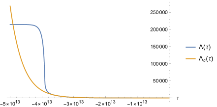
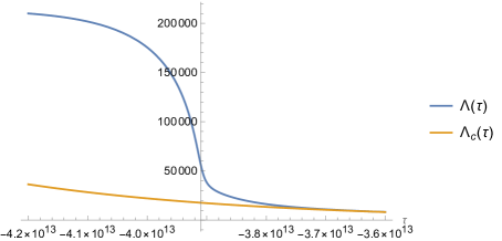
(c)	(d)
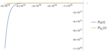
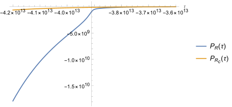
(e)	(f)
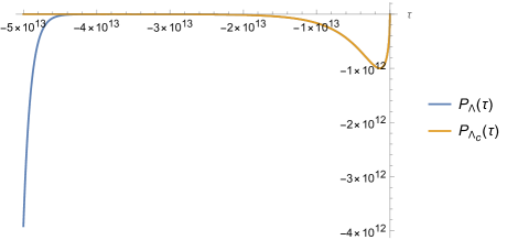
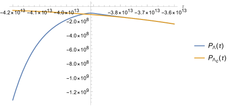
(g)	(h)

Figure 3: Plots of the physical variables $\left(R,\Lambda,P_{R},P_{\Lambda}\right)$ and their classical correspondences $\left(R_{c},\Lambda_{c},P_{R_{c}},P_{\Lambda_{c}}\right)$. Particular attention are paid to the region near the throat $\tau=-3.91\times 10^{13}$. Graphs are plotted with $m=10^{12}m_{p},\;j=j_{0}=10$.

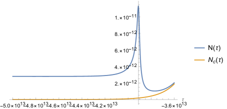
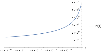
(a)	(b)
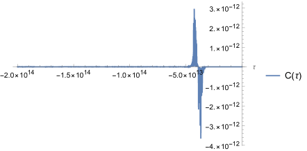
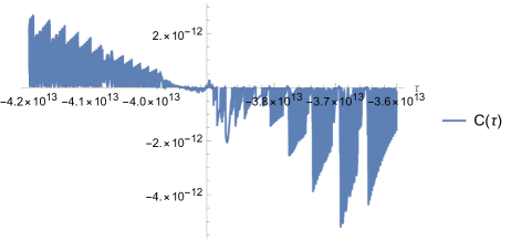
(c)	(d)

Figure 4: Plots of $\mathcal{C}(\tau)$ and the lapse function $N(\tau)$ for $m=10^{12}m_{p},\;j=j_{0}=10$.

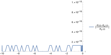
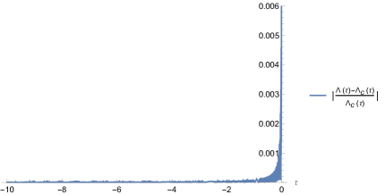
(a)	(b)
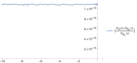
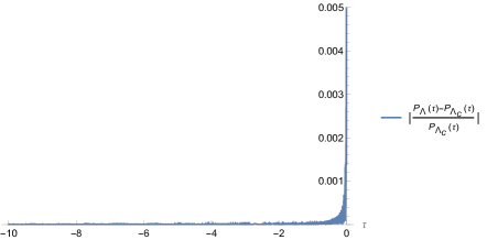
(c)	(d)
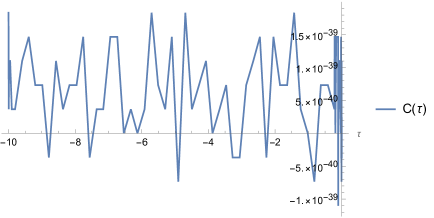
(e)	(f)

Figure 5: Plots of the relative differences of the functions $\left(R,\Lambda,P_{R},P_{\Lambda},N\right)$ and $\mathcal{C}(\tau)$ near the black hole horizon with the same choice of the parameters $m$ and $j$, as those specified in Figs. 3 and 4, that is, $m=10^{12}m_{p},\;j=j_{0}=10$.

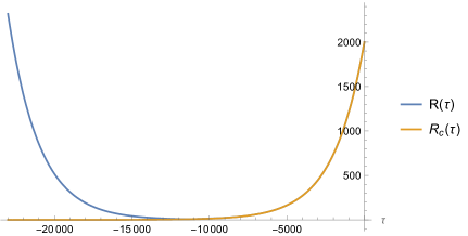
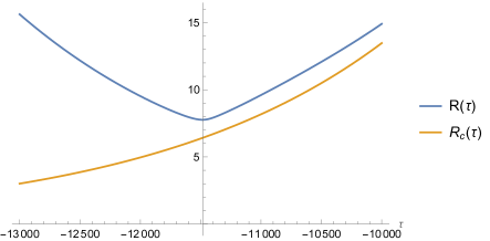
(a)	(b)
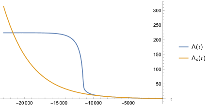
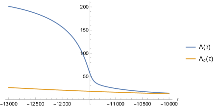
(c)	(d)
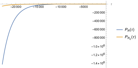
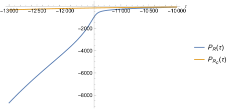
(e)	(f)
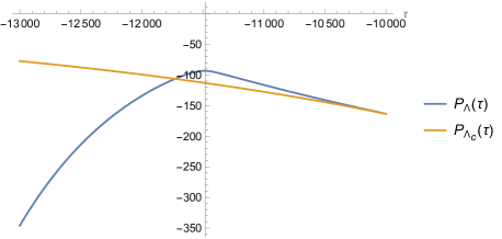
(g)	(h)

Figure 6: Plots of the physical variables $\left(R,\Lambda,P_{R},P_{\Lambda}\right)$ and their classical correspondences $\left(R_{c},\Lambda_{c},P_{R_{c}},P_{\Lambda_{c}}\right)$. Particular attention is paid to the region near the throat $\tau_{\text{min}}=-1.148\times 10^{4}$. Graphs are plotted with $m=10^{3}m_{p},\;j=j_{0}=10$.

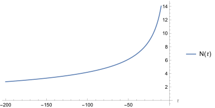
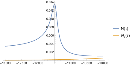
(a)	(b)
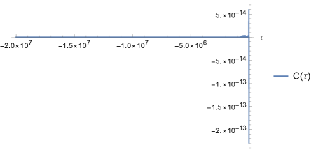
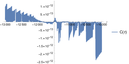
(c)	(d)

Figure 7: Plots of the lapse function $N(\tau)$ and $\mathcal{C}(\tau)$ for $m=10^{3}m_{p}$ and $j=j_{0}=10$.

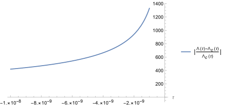
(a)	(b)
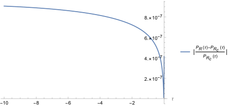
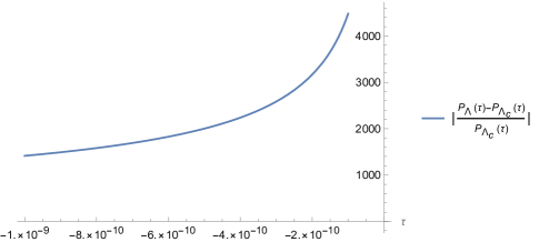
(c)	(d)
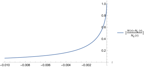
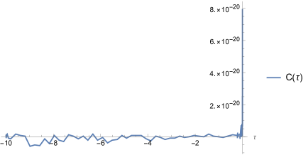
(e)	(f)

Figure 8: Plots of the relative differences of the functions $\left(R,\Lambda,P_{R},P_{\Lambda}\right)$, the lapse function $N(\tau)$ and $\mathcal{C}(\tau)$ near the black hole horizon ($\tau=0$) with $m=10^{3}m_{p}$ and $j=j_{0}=10$, the same choice as those specified in Figs. 6 and 7.

For the ABP model, we shall choose these three variables as $\left(R,\Lambda,P_{\Lambda}\right)$, so that

$$\Lambda(\tau_{i}) = \Lambda_{c}(\tau_{i}),\quad P_{\Lambda}(\tau_{i})=P_{\Lambda_{c}}(\tau_{i}),$$

$$R(\tau_{i}) = R_{c}(\tau_{i}),$$ (4.17)

while $P_{R}(\tau_{i})$ is obtained from the effective Hamiltonian constraint

$${\cal{H}}^{\text{IV+CS}}_{\text{int}}(\tau_{i})=0,\quad{\text{or}}\quad{\cal{C}}(\tau_{i})=0,$$ (4.18)

where ${\cal{C}}(\tau)$ is defined by Eq.(II.2). This reduced parameter space will be referred to as $\hat{\cal{D}}$. It is clear that this reduced space is much smaller than the whole phase space ${\cal{D}}$. However, for our current purpose, this is enough. With such chosen initial conditions, the Hamiltonian equations will uniquely determine the evolutions of the four variables ($\Lambda,P_{\Lambda}$) and ($R,P_{R}$) at any other time $\tau$. Once these four variables are known, from Eq.(2.24) we can find the lapse function $N(\tau)$.

With the above prescription, we can see that the initial values of the four variables will depend not only on the choice of the initial moment $\tau_{i}$ but also on the values of $j_{0},\;j$ and $m$. In particular, if the quantum effects are not negligible at the moment $\tau_{i}$, it is expected that such obtained $P_{R}(\tau_{i})$ should be significantly different from its corresponding relativistic value $P_{R_{c}}(\tau_{i})$.

To see this clearly, in Tables 1 - 3 we show such differences. In particular, in Table 1 we show the dependence of $P_{R}(\tau_{i})$ on the choice of the initial time $\tau_{i}$ for $m=10^{12}m_{p},\;j=j_{0}=10$. From this table we can see that $\Delta P_{R}(\tau_{i})\equiv P_{R}(\tau_{i})-P_{R_{c}}(\tau_{i})\simeq 0$ for $\tau_{i}/\tau_{p}\lesssim-0.1$. As $\tau_{i}\rightarrow 0$, the difference becomes larger.

In Table 2, we show the dependence of $P_{R}(\tau_{i})$ on the choices of $j$ with $m=10^{12}m_{p}$ and $\tau_{i}=-10.0\;\tau_{p}$. Physically, the lager the parameter $j$ is, the closer to the relativistic value of $P_{R}$ should be. However, due to the accuracy of the numerical computations, it is difficult to obtain precisely the values of $P_{R}$ from the effective Hamiltonian constraint (4.18). So, in Table 2 we only consider the initial values of $P_{R}(\tau_{i})$ for $j\lesssim 10^{12}$.

In Table 3, we show the dependence of $P_{R}(\tau_{i})$ on the choices of $m$ with $j=10$ and $\tau_{i}=-10.0\;\tau_{p}$, from which it can be seen that the deviations becomes larger for $m\lesssim 10^{3}\;m_{p}$. It should be also noted that for very large masses, the initial time $\tau_{i}$ must be chosen very negative. Otherwise, the term $e^{\tau/(Gm)}$, appearing in the effective Hamiltonian constraint [cf. Eqs.(3.12) - 3.14)], becomes extremely small, and numerical errors can be introduced. So, in Table 3 for the choice of $\tau_{i}=-10\tau_{p}$, we only consider the cases where $m$ is up to $10^{14}\;m_{p}$, although physically the larger $m$ is, the closer $P_{R}(\tau_{i})$ is to its relativistic values.

In Fig. 3, we plot the four functions $\left(R,\Lambda,P_{R},P_{\Lambda}\right)$, and their classical correspondences for $m=10^{12}m_{p},\;j=j_{0}=10,\;\tau_{i}=-10\;\tau_{p}$. With such initial conditions, we find that the location of throat (transition surface) is around $\tau_{\text{min}}\simeq-3.9108\times 10^{13}\tau_{p}$, at which $R(\tau)$ reaches its minimum value, $R_{\text{min}}\simeq 7779.35\;\ell_{p}$. It is interesting to note that near the throat the four functions all change dramatically, especially $\Lambda(\tau)$, which behaves like a step function. In addition, even at the transition surface, we find that the conditions of Eq.(2.16) are well satisfied.

To closely monitor the numerical errors, we also plot out the effective Hamiltonian (${\cal{C}}(\tau)\simeq 0$) in Fig. 4 together with the lapse function $N(\tau)$, from which we can see that in the region near the throat the numerical errors indeed become large. But out of this region, the numerical errors soon become negligible. From Fig. 3 and 4 we also find that our numerical solutions match well with their asymptotic behaviors given by Eq.(IV.1), as $\tau\rightarrow-\infty$.

To consider the quantum effects near the horizons, in Fig. 5 we plot out the relative differences between functions $\left(R,\Lambda,P_{R},P_{\Lambda},N\right)$ and their classical value. To monitor the numerical errors, we also plot out the effective Hamiltonian constraint ${\cal{C}}(\tau)\simeq 0$. From these plots, we can see clearly that the quantum effects indeed become negligible near the horizons .

On the other hand, when the mass of the black hole is near the Planck scale, such effects are not negligible even near the horizon. To show this, in Figs. 6 - 8 we plot various physical variables for $m=10^{3}\;m_{p},\;j=j_{0}=10$, for which we find that the location of throat is around $\tau_{\text{min}}\simeq-1.148\times 10^{4}\tau_{p}$, at which $R(\tau)$ reaches its minimum value, $R_{\text{min}}\simeq 7.76\;\ell_{p}$. From these figures it is clear that now the quantum effects become large near the horizons, and cannot be negligible. It should be noted that for such small black hole, the semi-classical limit conditions (IV.1) are not well satisfied at the throat, and as a result, the corresponding effective Hamiltonian may no longer describe the real quantum dynamics well. For more details, we refer readers to [62, 63].

IV.2 $\eta\gtrsim 1$

In this case, we find

$$X \simeq \eta_{0},\quad Y\simeq\frac{\eta_{0}}{\eta},$$

$$W \simeq \pi h_{0}[\eta_{0}]+2\sin[\eta_{0}],$$

$$\frac{P_{\Lambda}}{R^{2}} \simeq \frac{\eta_{0}}{\alpha\gamma G},\quad\frac{P_{R}}{R\Lambda}\simeq\frac{2\eta_{0}}{\alpha\gamma G},$$

as $\tau\rightarrow-\infty$. Then, the metric coefficients have the following asymptotical behavior,

$$N(\tau) \simeq N_{0}=-\frac{2\gamma\sqrt{8\pi\gamma}\;\ell_{p}\;\sqrt{j_{0}},}{mG\left(\pi h_{0}[\eta_{0}]+2\sin[\eta_{0}]\right)},$$

$$\Lambda(\tau) \simeq \Lambda_{0}\exp\left\{\frac{{\cal{F}}(\eta)}{2mG}\tau\right\},$$

$$R(\tau) \simeq R_{0}\exp\left\{\frac{\cos\left(\frac{\eta_{0}}{\eta}\right)}{2mG}\tau\right\},$$ (4.20)

where $\Lambda_{0}$ and $R_{0}$ are constants, and

$${\cal{F}}(\eta) = \frac{1}{{\mathcal{D}(\eta_{0})}^{2}}\Big{[}2\pi h_{-1}(\eta_{0})\sin^{2}(\eta_{0})+\pi^{2}\cos(\eta_{0})h_{0}^{2}(\eta_{0})\Big{]}$$ (4.21)

$$-\cos\left(\frac{\eta_{0}}{\eta}\right),$$

where ${\mathcal{D}(\eta_{0})}$ is defined by Eq.(2.33) but now with $A=B=0$, and the constant $\eta_{0}$ is implicitly determined by

$$\eta\sin\left(\frac{\eta_{0}}{\eta}\right)+\frac{\pi}{{\cal{D}}(\eta_{0})}\sin(\eta_{0})h_{0}(\eta_{0})=0.$$ (4.22)

In [62], it was shown that ${\cal{F}}(\eta)<0$ and $\eta_{0}<-\pi$ when $\eta>1$, so that both $R$ and $\Lambda$ grow exponentially as $\tau\rightarrow-\infty$. Setting

$$a\equiv\frac{\left|{\cal{F}}(\eta)\right|}{2mG}>0,\quad d\equiv\frac{\left|\cos\left(\frac{\eta_{0}}{\eta}\right)\right|}{2mG}>0,$$ (4.23)

we find that

$$\Lambda=\Lambda_{0}e^{-a\tau},\quad R=R_{0}e^{-d\tau}.$$ (4.24)

Then, the metric takes the following asymptotical form

$$ds^{2}\simeq-\left(\frac{\hat{N}_{0}}{R}\right)^{2}dR^{2}+R^{\frac{2a}{d}}d\bar{x}^{2}+R^{2}d\Omega^{2},$$ (4.25)

where $\hat{N}_{0}\equiv N_{0}/d$, but now with $\bar{x}\equiv\left(\Lambda_{0}/R_{0}^{a/d}\right)x$. Similar to the last case, the corresponding spacetime is not vacuum, and the effective energy-momentum tensor takes the same form as that given by Eq.(3.44), but now with $u_{\mu}=(\hat{N}_{0}/R)\delta^{R}_{\mu}$, $\bar{x}_{\mu}=R^{a/d}\delta^{\bar{x}}_{\mu}$, and

$$\rho \simeq \frac{2a+d}{d\hat{N}_{0}^{2}}+\frac{1}{R^{2}},$$

$$p_{\bar{x}} \simeq -\frac{3}{\hat{N}_{0}^{2}}-\frac{1}{R^{2}},$$

$$p_{\bot} \simeq -\frac{a^{2}+ad+d^{2}}{d^{2}\hat{N}_{0}^{2}},$$ (4.26)

from which we find that

$$\rho+p_{\bar{x}} \simeq \frac{2(a-d)}{d\hat{N}_{0}^{2}}+{\cal{O}}\left(\frac{1}{R^{2}}\right),$$

$$\rho+p_{\bot} \simeq -\frac{a(a-d)}{d^{2}\hat{N}_{0}^{2}}+{\cal{O}}\left(\frac{1}{R^{2}}\right).$$ (4.27)

Therefore, in this case none of the three energy conditions is satisfied either, provided that $a\not=d$. When $a=d$, the spacetime is asymptotically de Sitter, as shown below. In particular, we find that

$${\cal{R}}\simeq 2\left(\frac{a^{2}+2ad+3d^{2}}{d^{2}\hat{N}_{0}^{2}}+\frac{1}{R^{2}}\right),$$

$$R_{\mu\nu}R^{\mu\nu}\simeq 2\frac{a^{4}+2a^{3}d+5a^{2}d^{2}+4ad^{3}+6d^{4}}{d^{4}\hat{N}_{0}^{4}}$$

$$~{}~{}~{}~{}~{}~{}~{}~{}~{}~{}~{}~{}~{}~{}~{}~{}~{}~{}+\frac{4(a+2d)}{d\hat{N}_{0}^{2}R^{2}}+\frac{2}{R^{4}},$$

$$R_{\mu\nu\alpha\beta}R^{\mu\nu\alpha\beta}\simeq 4\frac{a^{4}+2a^{2}d^{2}+3d^{4}}{d^{4}\hat{N}_{0}^{4}}+\frac{8}{\hat{N}_{0}^{2}R^{2}}+\frac{4}{R^{4}},$$

$$C_{\mu\nu\alpha\beta}C^{\mu\nu\alpha\beta}\simeq\frac{4\left(aR^{2}(a-d)+d^{2}\hat{N}_{0}^{2}\right){}^{2}}{3d^{4}\hat{N}_{0}^{4}R^{4}}.$$ (4.28)

Therefore, different from the last case, asymptotically the spacetime is conformally flat only when $a=d$. Otherwise, we have $C_{\mu\nu\alpha\beta}C^{\mu\nu\alpha\beta}\simeq 4a^{2}(a-d)^{2}/(3d^{4}\hat{N}_{0}^{4})+\mathcal{O}\left(1/R^{2}\right)$.

On the other hand, introducing the quantity $\bar{t}$ via the relation

$$\bar{t}=-\frac{d\hat{N}_{0}}{aR^{a/d}_{0}}\left(\frac{R_{0}}{R}\right)^{a/d}\equiv-\bar{t}_{0}\left(\frac{R_{0}}{R}\right)^{a/d},$$ (4.29)

we find that the metric (4.25) takes the form

$$ds^{2}\simeq R_{0}^{2a/d}\left(\frac{\bar{t}_{0}}{\bar{t}}\right)^{2}\left(-d\bar{t}^{2}+d\bar{x}^{2}\right)+R^{2}d\Omega^{2}.$$ (4.30)

When $a=d$, Eq.(4.30) reduces to

$$ds^{2}\simeq R_{0}^{2}\left(\frac{\bar{t}_{0}}{\bar{t}}\right)^{2}\left(-d\bar{t}^{2}+d\bar{x}^{2}+d\Omega^{2}\right),\;(a=d),~{}~{}~{}~{}$$ (4.31)

which is the same as the de Sitter spacetime for $R\gg R_{\Lambda}$, where $R_{\Lambda}$ is the de Sitter radius. In fact, when $R\gg R_{\Lambda}$ we have that the de Sitter spacetime is given by

$$ds_{\Lambda}^{2} = -\left(1-\left(\frac{R}{R_{\Lambda}}\right)^{2}\right)d\bar{x}^{2}+\left(1-\left(\frac{R}{R_{\Lambda}}\right)^{2}\right)^{-1}dR^{2}$$ (4.32)

$$+R^{2}d\Omega^{2}$$

$$\simeq \left(\frac{R_{\Lambda}}{\bar{t}}\right)^{2}\Big{(}-d\bar{t}^{2}+d\bar{x}^{2}+d\Omega^{2}\Big{)},$$

but now with the rescaling $\bar{x}\rightarrow\bar{x}/R_{\Lambda}$ and

$$\bar{t}\equiv-\frac{R_{\Lambda}}{R}.$$ (4.33)

Note that the angular sectors of the two metrics (4.30) and (4.32) are different in terms of $\bar{t}$. In particular, in the metric (4.30) we have $R^{2}\propto(-\bar{t})^{-2d/a}$, while in the de Sitter spacetime we have $R^{2}\propto(-\bar{t})^{-2}$. Therefore, they are equal only when $a=d$. However, the sectors of the $(\bar{t},\bar{x}$)-planes are quite similar even when $a\not=d$. As a result, in both cases the surfaces $\bar{t}=0$ represent spacelike hypersurfaces and form the boundaries of the spacetimes. Then, the corresponding Penrose diagram in the current case is given by Fig. 9.

Figure 9: The Penrose diagram for the loop quantum spacetimes without the inverse volume corrections in the case $\eta>1$ (As to be shown below, the corresponding Penrose diagram for the case $\eta<1$ is also given by this figure). The curved lines denoted by $\tau_{b}$ are the transition surfaces (throats), and the straight lines AD and BC are the locations of the black hole horizons, while the straight lines AB and CD are the spacelike infinities, which correspond to $\bar{t}=0$ and form the future/past boundaries. The whole spacetime is free of singularities.

When $a=d$, since $\mathcal{F}(\eta)<0$ and $\cos\left(\frac{\eta_{0}}{\eta}\right)<0$, from Eq.(4.23) we find

$$\mathcal{F}(\eta)=\cos\left(\frac{\eta_{0}}{\eta}\right).$$ (4.34)

On the other hand, $\eta$ and $\eta_{0}$ must satisfy Eq.(4.22), too. So, these two equations uniquely determine $\eta$ and $\eta_{0}$. For $\eta_{0}\lesssim-\pi$, we find that Eqs.(4.22) and (4.34) have the solution,

$$\left(\eta,\eta_{0}\right)\approx\left(1.142,-3.329\right),$$ (4.35)

for which, from Eqs.(2.13) and (2.22) we find that

$$\gamma=\frac{\sqrt{2\pi}}{8\eta}\simeq 0.274.$$ (4.36)

It is remarkable to note that this value is precisely the one found from the analysis of black hole entropy [64]. It should be also noted that Eqs.(4.22) and (4.34) have multi-valued solutions, as these two equations are involved with periodic functions. In this paper, we consider only the case $\eta_{0}\lesssim-\pi$ [62].

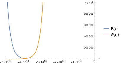
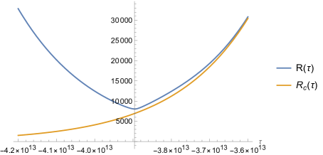
(a)	(b)
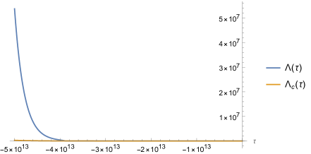
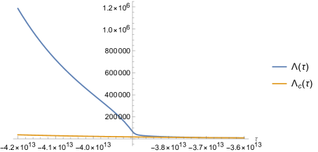
(c)	(d)
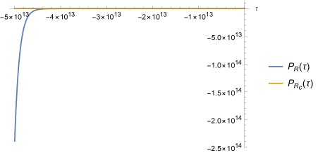
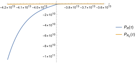
(e)	(f)
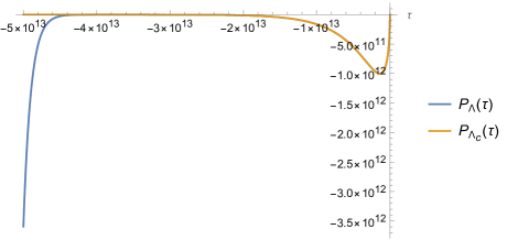
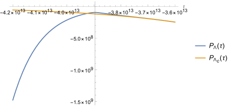
(g)	(h)

Figure 10: Plots of the physical variables $\left(R,\Lambda,P_{R},P_{\Lambda}\right)$ and their classical correspondences $\left(R_{c},\Lambda_{c},P_{R_{c}},P_{\Lambda_{c}}\right)$. Particular attention is paid to the region near the throat $\tau_{\text{min}}=-3.896\times 10^{13}$, at which $R(\tau)=8059.95$. Graphs are plotted with $m=10^{12}m_{p},\;j_{0}=11.42,\;j=10,\;\eta=1.142$.

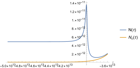
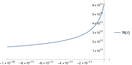
(a)	(b)
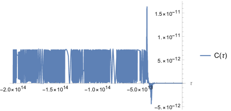
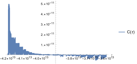
(c)	(d)

Figure 11: Plots of $\mathcal{C}(\tau)$ and the lapse function $N(\tau)$ for $m=10^{12}m_{p},\;j_{0}=11.42,\;j=10,\;\eta=1.142$.

(a)	(b)
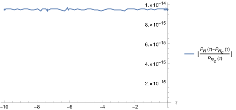
(c)	(d)
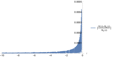
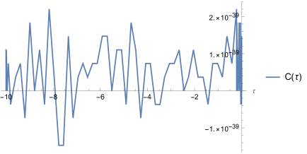
(e)	(f)

Figure 12: Plots of the relative differences of the functions $\left(R,\Lambda,P_{R},P_{\Lambda},N(\tau)\right)$ and $\mathcal{C}(\tau)$ near the black hole horizon with the same choice of the parameters $m$ and $j$, as those specified in Figs. 10 and 11, that is, $m=10^{12}m_{p},\;j_{0}=11.42,\;j=10,\;\eta=1.142$.

Table 4: The dependence of the constants $N_{0}$, $R_{0}$, $\Lambda_{0}$ of Eq.(IV.1) on $m$ with $\eta\approx 1.142,\;\gamma\approx 0.274,\;j_{x}=10^{5}$. The corresponding transition times $\tau_{\text{min}}$ and radii $R_{\text{min}}$ are also given.

$\frac{m}{m_{p}}$	$~{}~{}~{}~{}~{}~{}\frac{\tau_{\text{min}}}{\tau_{p}}$	$\frac{R_{\text{min}}}{\ell_{p}}$	$~{}~{}~{}~{}~{}~{}~{}N_{0}$	$R_{0}$	$\Lambda_{0}$
$10^{12}$	$-3.260\times 10^{13}$	193114	$5.706\times 10^{-10}$	0.0226	0.00725
$10^{10}$	$-2.646\times 10^{11}$	41605.1	$5.706\times 10^{-8}$	0.0968	0.0311
$10^{6}$	$-1.418\times 10^{7}$	1929.73	$5.706\times 10^{-4}$	1.787	0.631

In Figs. 10 - 12, we plot various physical quantities for $m=10^{12}m_{p},\;j_{0}=11.42,\;j=10$, so that $\eta\equiv j_{0}/j=1.142$. This corresponds to the case studied in [63], which will be analyzed in more detail in the next section with $ABC\not=0$. Then, we find that the transition surface is located at $\tau_{\text{min}}/\tau_{p}\simeq-3.896\times 10^{13}$, at which we have $R(\tau_{\text{min}})\simeq 8059.95$. Note that with these choices of $m,\;j$ and $j_{x}$, the semiclassical limit conditions (2.14) and (2.16) are well satisfied. Then, from Figs. 10 and 11 we find that the asymptotical behavior of the metric coefficients given by Eq.(IV.1) is well justified, while Fig. 12 shows that the quantum effects near the black hole horizon ($\tau\simeq 0$) are negligible even for $m/m_{p}=10^{12}$. For the cases with solar mass $m/m_{p}\gtrsim 10^{38}$, it is expected that such effects are even smaller.

It should be noted that the specific values of the factors $N_{0},R_{0}$ and $\Lambda_{0}$ appearing in Eq.(IV.1) depend on the choice of $m$, although the asymptotic behavior of $N,R$ and $\Lambda$ all take the form of Eq.(IV.1). As a result, the corresponding Penrose diagram is the same and given by Fig. 9 for any given $\eta>1$. In Table 4 we present their values for several choices of $m$.

We also study the effects of $\eta$, and find that the quality behaviors of the spacetimes are quite similar to the above even when $\eta=2$, as long as the semiclassical limit conditions (2.14) and (2.16) are satisfied and $m$ is not too small ($m/m_{p}\gtrsim 10^{6}$).

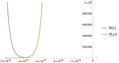
(a)	(b)
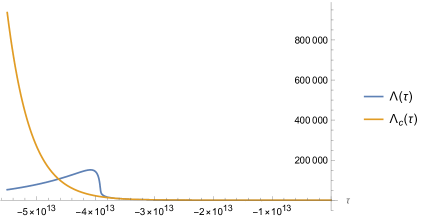
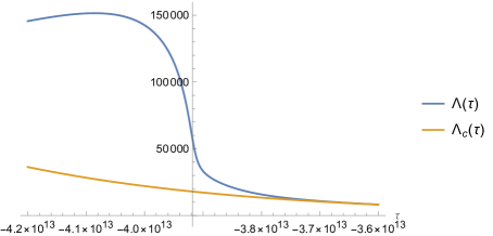
(c)	(d)
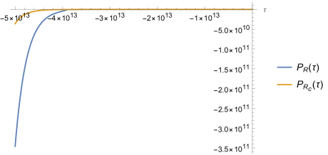
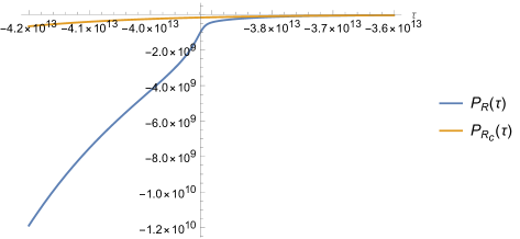
(e)	(f)
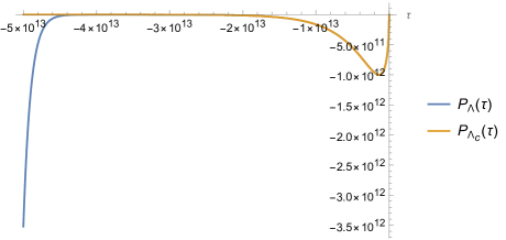
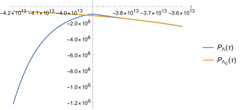
(g)	(h)

Figure 13: Plots of the physical variables $\left(R,\Lambda,P_{R},P_{\Lambda}\right)$ and their classical correspondences $\left(R_{c},\Lambda_{c},P_{R_{c}},P_{\Lambda_{c}}\right)$. Particular attention is paid to the region near the throat $\tau_{\text{min}}=-3.918\times 10^{13}$, at which $R(\tau_{\text{min}})=7676.1$. Graphs are plotted with $m=10^{12}m_{p},\;j_{0}=9.5,\;j=10,\;\eta=0.95$.

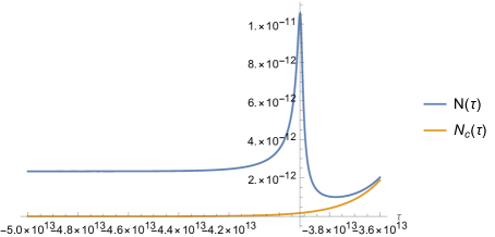
(a)	(b)
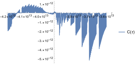
(c)	(d)

Figure 14: Plots of $\mathcal{C}(\tau)$ and the lapse function $N(\tau)$ for $m=10^{12}m_{p},\;j_{0}=9.5,\;j=10,\;\eta=0.95$.

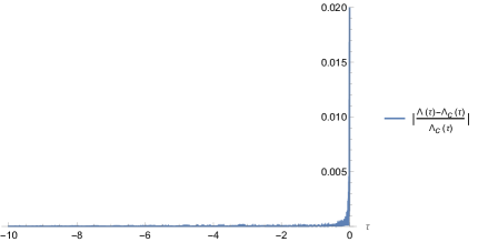
(a)	(b)
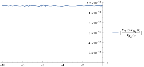
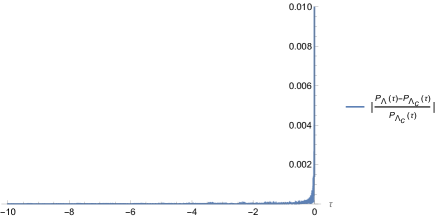
(c)	(d)
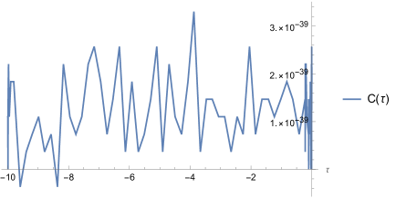
(e)	(f)

Figure 15: Plots of the relative differences of the functions $\left(R,\Lambda,P_{R},P_{\Lambda},N(\tau)\right)$ and $\mathcal{C}(\tau)$ near the black hole horizon with the same choice of the parameters $m$ and $j$, as those specified in Figs. 13 and 14, that is, $m=10^{12}m_{p},\;j_{0}=9.5,\;j=10,\;\eta=0.95$.

IV.3 $\eta\lesssim 1$

When $\eta\lesssim 1$, the metric coefficients take the same asymptotical forms as those given by Eqs.(IV.1) - (4.22), but now with ${\cal{F}}(\eta)>0$ and $\eta_{0}>-\pi$ [62]. Therefore, now $\Lambda$ decreases exponentially as $\tau\rightarrow-\infty$, while $R$ still keeps increasing exponentially, i.e.

$$N \simeq -\frac{2\gamma\sqrt{8\pi\gamma}\;\ell_{p}\;\sqrt{j_{0}},}{mG\left(\pi h_{0}[\eta_{0}]+2\sin[\eta_{0}]\right)},$$

$$\Lambda = \Lambda_{0}e^{a\tau},\quad R=R_{0}e^{-d\tau}.$$ (4.37)

Then, the metric takes the following asymptotical form

$$ds^{2}\simeq-\left(\frac{\hat{N}_{0}}{R}\right)^{2}dR^{2}+\frac{d\bar{x}^{2}}{R^{{2a}/{d}}}+R^{2}d\Omega^{2}.$$ (4.38)

The corresponding effective energy-momentum tensor also takes the same form as that given by Eq.(3.44), but now with $u_{\mu}=(\hat{N}_{0}/R)\delta^{R}_{\mu}$, $\bar{x}_{\mu}=R^{-a/b}\delta^{\bar{x}}_{\mu}$, and

$$\rho \simeq \frac{d-2a}{d\hat{N}_{0}^{2}}-\frac{1}{R^{2}},$$

$$p_{\bar{x}} \simeq -\frac{3}{\hat{N}_{0}^{2}}-\frac{1}{R^{2}},$$

$$p_{\bot} \simeq -\frac{a^{2}-ad+d^{2}}{d^{2}\hat{N}_{0}^{2}},$$ (4.39)

from which we can see that none of the three energy conditions are satisfied for any given $a$ and $d$. In particular, when $a=d$ we have $\rho\simeq p_{\bar{x}}/3\simeq p_{\bot}<0$. In addition, we also have

$${\cal{R}}\simeq 2\left(\frac{a^{2}-2ad+3d^{2}}{d^{2}\hat{N}_{0}^{2}}+\frac{1}{R^{2}}\right),$$

$$R_{\mu\nu}R^{\mu\nu}\simeq 2\frac{a^{4}-2a^{3}d+5a^{2}d^{2}-4ad^{3}+6d^{4}}{d^{4}\hat{N}_{0}^{4}}-\frac{4(a-2d)}{d\hat{N}_{0}^{2}R^{2}}+\frac{2}{R^{4}},$$

$$R_{\mu\nu\alpha\beta}R^{\mu\nu\alpha\beta}\simeq 4\left(\frac{a^{4}+2a^{2}d^{2}+3d^{4}}{d^{4}\hat{N}_{0}^{4}}+\frac{2}{\hat{N}_{0}^{2}R^{2}}+\frac{1}{R^{4}}\right),$$

$$C_{\mu\nu\alpha\beta}C^{\mu\nu\alpha\beta}\simeq\frac{4\left(aR^{2}(a+d)+d^{2}\hat{N}_{0}^{2}\right){}^{2}}{3d^{4}\hat{N}_{0}^{4}R^{4}},$$ (4.40)

which can be obtained from Eq.(IV.1) by the replacement $a\rightarrow-a$, as expected.

To consider the corresponding Penrose diagram, we first write the metric (4.38) in the form

$$ds^{2}\simeq-R_{0}^{-2a/d}\left(\frac{\bar{t}_{0}}{\bar{t}}\right)^{2}\left(-d\bar{t}^{2}+d\bar{x}^{2}\right)+R^{2}d\Omega^{2},$$ (4.41)

where

$$\bar{t} = \bar{t}_{0}\left(\frac{R}{R_{0}}\right)^{a/d},\quad\bar{x}\equiv\left(\Lambda_{0}R_{0}^{a/d}\right)x,$$

$$R = R_{0}\left(\frac{\bar{t}}{\bar{t}_{0}}\right)^{d/a},\;\;\bar{t}_{0}\equiv\frac{d\hat{N}_{0}R^{a/d}_{0}}{a}.$$ (4.42)

Comparing Eq.(4.41) with Eq.(4.30), we find that the ($\bar{t},\bar{x}$)-planes in both spacetimes have the same structure, and the only difference is to replace $a$ by $-a$. Thus, the corresponding Penrose diagram is also given by Fig. 9. It is interesting to note that now the spacetime is not asymptotically de Sitter, even when $a=d$. In fact, now it is even not asymptotically conformally flat as can be seen from Eq.(IV.3). In addition, in the current case none of the three energy conditions are satisfied.

In Figs. 13 - 15, we plot various physical quantities for $m/m_{p}=10^{12},\;j_{0}=9.5,\;j=10$ so that $\eta\equiv j_{0}/j=0.95<1$. In this case, the transition surface is located at $\tau_{\text{min}}=-3.918\times 10^{13}$, at which we find $R(\tau_{\text{min}})=7676.1$. Then, it can be shown that both of the conditions (2.14) and (2.16) are satisfied. Therefore, the corresponding semiclassical description of the quantum black holes is well justified. In particular, from Figs. 13 and 14 we find that the asymptotic behavior of the metric coefficients are well approximated by Eq.(IV.3), while Fig. 15 shows that near the horizon ($\tau\simeq 0$) the quantum geometric effects become negligible, possibly except the region very near to the horizon [cf. Fig. 15].

It is interesting to note that the asymptotic behavior in the current case is very sensitive to the choice of $\eta$. In particular, we find that when $\eta=0.5$ the asymptotic behavior of the spacetime is already quite different from the one described by Eq.(IV.3), although the semiclassical conditions (2.14) and (2.16) are still well justified.

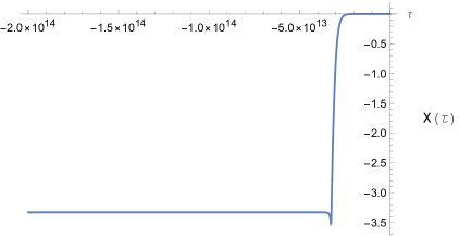
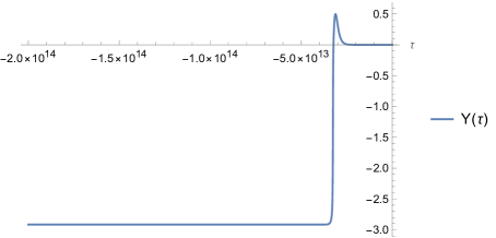
(a)	(b)
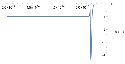
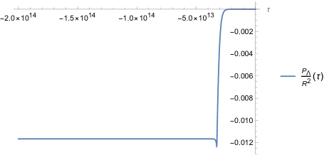
(c)	(d)
(e)

Figure 16: Plots of the functions $\left(X,Y,W,\frac{P_{\Lambda}}{R^{2}},\frac{P_{R}}{R\Lambda}\right)$. The throat is lcated at $\tau_{\text{min}}=-3.260\times 10^{13}$, at which $R(\tau_{\text{min}})=193115$. Curves are plotted with $\gamma\approx 0.274,\;m=10^{12}m_{p},\;j_{x}=10^{5},\;\eta\approx 1.142$.

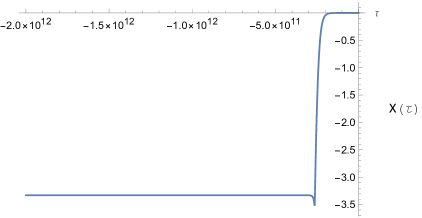
(a)	(b)
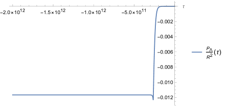
(c)	(d)
(e)

Figure 17: Plots of the functions $\left(X,Y,W,\frac{P_{\Lambda}}{R^{2}},\frac{P_{R}}{R\Lambda}\right)$. The throat is at $\tau_{\text{min}}=-2.646\times 10^{11}$, at which $R(\tau_{\text{min}})=41609.4$. Graphs are plotted with $\gamma\approx 0.274,\;m=10^{10}m_{p},\;j_{x}=10^{5},\;\eta\approx 1.142$.

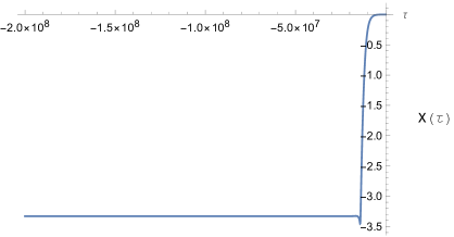
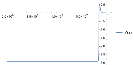
(a)	(b)
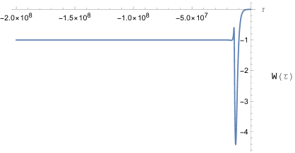
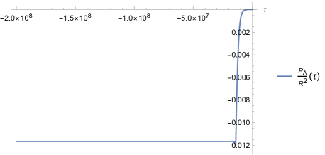
(c)	(d)
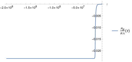
(e)

Figure 18: Plots of the functions $\left(X,Y,W,\frac{P_{\Lambda}}{R^{2}},\frac{P_{R}}{R\Lambda}\right)$. The throat is at $\tau_{\text{min}}=-1.416\times 10^{7}$, at which $R(\tau_{\text{min}})=2012.19$. Graphs are plotted with $\gamma\approx 0.274,\;m=10^{6}m_{p},\;j_{x}=10^{5},\;\eta\approx 1.142$.

V Main Properties of the quantum reduced loop Black Holes with the Inverse Volume Corrections

As shown in [63], the inverse volume corrections, represented by terms proportional to the constants $A,B$ and $C$ in the effective Hamiltonian given by Eqs.(2.10) and (II.2), are sub-leading. This can be also seen clearly from the analysis given in the beginning of the last section. Therefore, the inverse volume corrections should not change the main properties of the solutions with $\eta=1,\;\eta>1,\;\eta<1$, respectively. However, demanding that the spatial manifold triangulation remain consistent on both sides of the black hole horizons, ABP found [63]

$$j=\gamma j_{x},$$ (5.1)

which immediately leads to

$$\eta\equiv\frac{\alpha}{\beta}=\frac{\sqrt{2\pi}}{8\gamma},$$ (5.2)

as can be seen from Eq.(2.13). On the other hand, the considerations of black hole entropy in LQG showed that [64]

$$\gamma\simeq 0.274,$$ (5.3)

which is precisely the solution obtained by requiring $a=d$ in Section IV.B for the case $\eta>1$, in order to have the spacetime on the other side of the transition surface to be de Sitter, where $a$ and $b$ are the constants defined in Eq.(4.23). This “surprising coincidence” was first noted in [63] with a different approach, but in this paper we obtained it simply by requiring that the transition surface connect two regions, one is asymptotically the Schwarzschild and the other is de Sitter. Therefore, following [63] in this section we consider only the case $\gamma\simeq 0.274$ , for which we have $\eta\simeq 1.142$.

Once $\gamma$ and $\eta$ are fixed, the five-parameter solutions of ABP are uniquely determined, after the inverse value correction parameters $\nu,\delta$ and $\delta_{x}$ are given. In the following, we adopt the values given by ABP [63],

$$\nu = 1.802,\quad\delta=\frac{1.458}{\beta^{2}}+{\cal{O}}\left(\beta^{-6}\right),$$

$$\delta_{x} = \frac{0.729}{\beta^{2}}+{\cal{O}}\left(\beta^{-6}\right).$$ (5.4)

In Figs. 16 - 18, we plot out the functions $\left(X,\;Y,\;W,\;\frac{P_{\Lambda}}{R^{2}},\;\frac{P_{R}}{R\Lambda}\right)$, for different $m$. From these figures we find

$$X \simeq -\iota\approx-3.329,\quad Y\simeq-\frac{\iota}{\eta}\approx-2.915,$$

$$W \simeq -(\pi h_{0}[\iota]+2\sin[\iota])\approx-1.001,$$

$$\frac{P_{\Lambda}}{R^{2}} \simeq -\frac{\iota}{\alpha\gamma G}\approx-0.012,$$

$$\frac{P_{R}}{R\Lambda} \simeq -\frac{2\iota}{\alpha\gamma G}\approx-0.023,$$ (5.5)

as $\tau\rightarrow-\infty$, where $\iota\equiv-\eta_{0}\simeq 3.329$ [63]. With the above expressions, we find that the asymptotical behavior of $N(\tau),R(\tau)$ and $\Lambda(\tau)$ is precisely given by Eq.(IV.2), with the dependence of the three constants $N_{0},\;R_{0}$ and $\Lambda_{0}$ being given by Table 4.

As shown in Sec. IV.B for the case $\eta>1$, the inverse volume corrections become important only when the geometric radius $R$ is in the order of the Planck scale, $R\simeq\ell_{p}$. However, for macroscopic black holes, the radius of the transition surface $R_{\text{min}}$ is always much larger than $\ell_{p}$. For example, when $m/m_{p}=10^{12}$, $R_{\text{min}}/\ell_{p}\simeq 8059.95\gg 1$ [cf. Fig. 10]. Therefore, for macroscopic black holes the inverse volume corrections can be safely neglected. This is true not only for the case $\eta=1.142$, but also true for all the cases considered in Sec. IV for macroscopic black holes. Therefore, in this section we shall not repeat our analyses carried out in that section.

VI Concluding Remarks

In this paper, we systematically study quantum black holes in the framework of QRLG, proposed recently by ABP [61, 62, 63]. Starting from the full theory of LQG, ABP derived the effective Hamiltonian with respect to coherent states peaked around spherically symmetric geometry, by including both the holonomy and inverse volume corrections. Then, they showed that the classical singularity used to appear inside the Schwarzschild black hole is replaced by a regular transition surface with a finite and non-zero radius.

To understand such obtained effective Hamiltonian well and shed light on the relations to models obtained by the bottom-up approach, in Sec. III.1 we first consider its classical limit, and obtained the desired Schwarzschild black hole solution, whereby the physical and geometric interpretation of the quantities used in the effective Hamiltonian are made clear. Then, in Sec. III.2 and Sec. III.3 by taking proper limits we re-derive respectively the BV [13] and AOS [30, 31, 40] solutions, all obtained by the bottom-up approach. In doing so, we can see clearly the relation between models obtained by the two different approaches, top-down and bottom-up.

In particular, the BV effective Hamiltonian was originally obtained from the classical Hamiltonian (2.7) with the polymerization,

$$b\rightarrow\frac{\sin(\delta_{b}b)}{\delta_{b}},\quad c\rightarrow\frac{\sin(\delta_{c}c)}{\delta_{c}}.$$ (6.1)

However, instead of taking the parameters $\delta_{b}$ and $\delta_{c}$ as constants, following the $\bar{\mu}$-scheme first proposed in LQC [12] , BV took them as

$$\delta_{b}^{\text{(BV)}}=\sqrt{\frac{\Delta}{p_{c}}},\quad\delta_{c}^{\text{(BV)}}=\frac{\sqrt{\Delta p_{c}}}{p_{b}}.$$ (6.2)

In Sec. III.B, we show explicitly that the BV effective Hamiltonian can be obtained from the ABP Hamiltonian by taking the following replacement and limit,

$$(i)\;h_{0}[X]\rightarrow\frac{2}{\pi}\sin[X],\quad h_{-1}[X]\rightarrow\frac{2}{\pi}\cos[X],$$ (6.3)

$$(ii)\;\frac{A}{R^{2}},\;\frac{B}{R^{2}},\;\frac{C}{R^{2}}\ll 1.$$ (6.4)

It should be noted that with the choice of Eq.(6.2), the corresponding values of $j_{x}$ and $j$ are given by Eq.(III.2), from which we can see that they all violate the semi-classical limit (2.14), with which the ABP effective Hamiltonian (2.10) was derived. As a result, the BV model cannot be physically realized in the framework of QRLG, although formally they can be obtained from the ABP effective Hamiltonian by the above replacement and limit.

On the other hand, in addition to the replacement and limit given respectively by Eqs.(6.3) and (6.4), if we further assume that

$$\delta^{\text{(AOS)}}_{b},\;\;\;\delta^{\text{(AOS)}}_{c}=\text{Constants},$$ (6.5)

and are determined by Eqs.(3.62) and (3.63), the ABP effective Hamiltonian (2.10) reduces precisely to the AOS one [30, 31, 40]. However, as shown explicitly by Eq.(III.3), such choices are also out of the semi-classical limit (III.2). Therefore, the AOS model cannot be realized in the framework of QRLG either.

It must be noted that the above conclusions do not imply that the BV and AOS models are unphysical, but rather than the fact that they must be realized in a different top-down approach.

With the above in mind, in Sec. IV we study the ABP effective Hamiltonian without the inverse volume corrections, represented by the $A,B,C$ terms in Eq.(2.10) in detail, by first confirming the main conclusions obtained in [62] and then clarifying some silent points. In particular, we find that the spacetime on the other side of the transition surface (throat) indeed sensitively depends on the ratio $\eta\equiv\alpha/\beta$, where $\alpha$ and $\beta$ are defined by Eq.(2.13) in terms of $(j_{x},\;j)$, or Eq.(4.1) in terms of $(\hat{j}_{0},\;\hat{j})$, where the parameters $(j_{x},\;j)$ were introduced in [63], while $(\hat{j}_{0},\;\hat{j})$ were used in [62], and related one to the other through Eq.(2.23). As noticed previously, in Sec. IV we drop the hats from $(\hat{j}_{0},\;\hat{j})\rightarrow(j_{0},\;j)$, for the sake of simplicity.

When $\eta=1$, the spacetime on the other side of the transition surface is conformally flat, and the non-vanishing curvatures are all of the order of the Planck scale, as can be seen from Eq.(IV.1). Then, the corresponding Penrose diagram is given by Fig. 2. At this point, we find that it is very helpful to make a closer comparison of the ABP model with the BV one, as for the BV choice of Eq.(3.34), we have $\eta^{\text{(BV)}}=1$. In particular, we find the following:

• In both models, the spacetime singularity used to appear at the center is replaced by a transition surface with a finite non-zero radius.

• In both models, the spacetime on one side of the transition surface is quite similar to the internal region of a Schwarzschild black hole with a black hole like horizon located at a finite distance from the transition surface (but with the removal of the black hole singularity used to occur at the center).

• In both models, the spacetime is asymmetric with respect to the transition surface, and model-dependent. In particular, in the BV model, the spacetime on the other side of the black hole like internal region approaches asymptotically to a charged Nariai space [68, 69, 70], of which the radius of the two-sphere $S^{2}$ approaches to a Planck scale constant, $R\rightarrow R_{0}\simeq{\cal{O}}(\ell_{p})$. In contrast, in the ABP model the radius grows exponentially without limits, $R\rightarrow\exp\left(-\frac{\tau}{2mG}\right)$ as $\tau\rightarrow-\infty$, and a macroscopic universe is obtained. The corresponding global structure can be seen clearly from its Penrose diagram given by Fig. 2.

• In the BV model, there exists multiple transition surfaces at which we have $dp_{c}/d\tau=0$. When passing each transition surface, $p_{c}$ decreases. As a result, $p_{c}$ will soon decreases to a value at which the two-spheres $S^{2}$ have areas smaller than $\Delta$, whereby the effective Hamiltonian is no longer valid. On the other hand, in the ABP model, only one such transition surface exists, and the above mentioned problem is absent. As a matter of fact, the two-planes spanned by $\tau$ and $x$ are asymptotically flat, as shown explicitly by Eq.(4.10), although the four-dimensional spacetime is not [cf. Eq.(IV.1)].

When $\eta\gtrsim 1$, the spacetime in general does not become conformally flat, as can seen from Eq.(IV.2), unless $a=d$, where $a$ and $d$ are two constants defined by Eq.(4.23). Then, the corresponding Penrose diagram is given by Fig. 9. When

$$a=d,$$ (6.6)

the spacetime is conformally flat and asymptotically de Sitter. It is remarkable that the condition (6.6) together with the one (2.21) leads to

$$\gamma=\frac{\sqrt{2\pi}}{8\eta}\simeq 0.274,$$ (6.7)

which is precisely the value obtained from the consideration of loop quantum black hole entropy obtained in [64]. As emphasized in [63], this coincidence should not be underestimated, and may provide some profound physics. In particular, the above picture is also consistent with the recently emerging picture in modified LQC models [73], in which the quantum bounce, which corresponds to the current transition surface, connects two regions, one is asymptotically de Sitter, and the other is asymptotically relativistic, after considering the expectation values of the Hamiltonian operator in LQG [74, 75, 76], by using complexifier coherent states [77], as shown explicitly in [78, 79, 80]. In addition, a similar structure of the spacetime of a spherical black hole also emerges in the framework of string [81], but now the transition surface is replaced by an S-Brane.

When $\eta\lesssim 1$, the spacetime cannot be conformally flat for any given values of $a$ and $d$, as it can be seen from Eq.(IV.3). However, the corresponding Penrose diagram is the same as that of the case with $\eta\gtrsim 1$, and given precisely by Fig. 9.

In review of all the above three cases, it is clear that the spacetime on the other side of the transition surface is no longer a white hole structure without spacetime singularities, as obtained from most of the bottom-up models [46, 41, 51], so that the corresponding Penrose diagram is extended repeatedly along the vertical line to include infinite identical universes of black holes and white holes (without spacetime singularities). Instead, the white hole region is replaced by either a conformally flat spacetime or a non-conformally flat one, given respectively by Figs. 2 and 9. But, in any case the spacetime is already geodesically complete, and no extensions are needed beyond their boundaries, so that in this framework multiple identical universes do not exist.

In addition, the undesirable feature in the BV model that multiple horizons exist on the other side of the transition surface disappears in the ABP model. In this model, the large quantum gravitational effects near the black hole horizons seemingly do not exist either, despite the fact that our numerical computations show that deviations may exist when very near to the black hole horizons, as shown explicitly in Figs. 5, 12, and 15. However, more careful analysis is required, as the metric becomes singular when crossing the horizons, and our numerical simulations may become unreliable. We wish to come back to this important question in another occasion.

When inverse volume corrections, represented by terms proportional to the constants $A,B,C$ in the effective Hamiltonian (2.10), are taken into account, the effects are always sub-leading, as these terms become important only when the radius of the two-sphere $\tau,x=$ Constant is of the order of the Planck scale. For macroscopic black holes, we find that the corresponding radii of the transition surfaces are always much larger than the Planck scale, so their effects will be always sub-leading even when across the transition surface. Such analysis was carried out in Sec. V, in which we mainly focus on the case in which the conditions (6.6) and (6.7) hold. In [63] it was shown that these sub-leading terms precisely make up all the requirement for a spacetime to be asymptotically de Sitter, defined in [82], even to the sub-leading order.

Appendix A Some properties of the Struve functions

In general, the $\nu$-th order Struve function $h_{\nu}[X]$ is defined as [67],

$$h_{\nu}[z]\equiv\left(\frac{1}{2}z\right)^{\nu+1}\sum_{k=0}^{\infty}{\frac{(-1)^{k}\left(\frac{1}{2}z\right)^{2k}}{\Gamma\left(k+\frac{3}{2}\right)\Gamma\left(k+\nu\frac{3}{2}\right)}},$$ (A.1)

which satisfies the differential equation,

$$z^{2}\frac{d^{2}w}{dz^{2}}+z\frac{dw}{dz}+\left(z^{2}-\nu^{2}\right)w=\frac{4\left(\frac{1}{2}z\right)^{\nu+1}}{\sqrt{\pi}\;\Gamma\left(\nu+\frac{1}{2}\right)}.$$ (A.2)

The general solution of the above equation is

$$w=aJ_{\nu}(z)+bY_{\nu}(z)+h_{\nu}(z),$$ (A.3)

where $a$ and $b$ are two integration constants, $J_{\nu}(z)$ and $Y_{\nu}(z)$ are the Bessel functions of the first and second kind, respectively, and satisfy the associated homogeneous differential equation.

Some useful properties of $h_{\nu}(z)$ are,

$$\frac{d\left(z^{\nu}h_{\nu}\right)}{dz} = z^{\nu}h_{\nu-1},$$

$$\frac{d\left(z^{-\nu}h_{\nu}\right)}{dz} = \frac{1}{\sqrt{\pi}\;2^{\nu}\;\Gamma\left(\nu+\frac{3}{2}\right)}-z^{-\nu}h_{\nu+1},$$ (A.4)

while their asymptotic behaviors are given by

$$h_{0}[X] \simeq \begin{cases}\frac{2}{\pi X}+\frac{1}{\sqrt{\pi X}}\left(\sin X-\cos X\right)+{\cal{O}}\left(X^{-3/2}\right),&X\rightarrow\infty,\cr\frac{2X}{\pi}-\frac{2X^{3}}{9\pi}+{\cal{O}}\left(X^{4}\right),&X\rightarrow 0,\cr\end{cases}$$ (A.5)

and

$$h_{-1}[X] \simeq \begin{cases}\frac{2}{\pi X}+\frac{1}{\sqrt{\pi X}}\left(\sin X+\cos X\right)+{\cal{O}}\left(X^{-3/2}\right),&X\rightarrow\infty,\cr\frac{2}{\pi}-\frac{2X^{2}}{3\pi}+{\cal{O}}\left(X^{4}\right),&X\rightarrow 0.\cr\end{cases}$$ (A.6)

In Fig. 1, we plot out the Struve function $h_{0}$ together with $h_{-1}$. For other properties of the Struve functions, we refer readers to [67].

References

- [1] T. Thiemann, Modern canonical quantum general relativity (Cambridge University Press, Cambridge, 2008).
- [2] M. Bojowald, Absence of singularity in loop quantum cosmology, Phys. Rev. Lett. 86, 5227 (2001).
- [3] M. Bojowald, Isotropic loop quantum cosmology, Class. Quant. Grav. 19, 2717 (2002).
- [4] A. Ashtekar and P. Singh, Loop Quantum Cosmology: A Status Report, Class. Quant. Grav. 28, 213001 (2011).
- [5] A. Ashtekar and B. Gupt, Quantum Gravity in the Sky: Interplay between fundamental theory and observations, Class. Quant. Grav. 34, 014002 (2017).
- [6] I. Agullo, A. Ashtekar and B. Gupt, Phenomenology with fluctuating quantum geometries in loop quantum cosmology, Class. Quant. Grav. 34, 074003 (2017).
- [7] A. Ashtekar, B. Gupt and V. Sreenath, Cosmic Tango Between the Very Small and the Very Large: Addressing CMB Anomalies Through Loop Quantum Cosmology, Front. Astron. Space Sci. 8, 76 (2021).
- [8] A. Corichi, T. Vukasinac and J. A. Zapata, Polymer Quantum Mechanics and its Continuum Limit, Phys. Rev. D 76, 044016 (2007).
- [9] A. Ashtekar and M. Bojowald, Quantum geometry and the Schwarzschild singularity, Class. Quant. Grav. 23, 391 (2006).
- [10] L. Modesto, Loop quantum black hole, Class. Quant. Grav. 23, 5587 (2006).
- [11] A. Ashtekar, A. Corichi and P. Singh, Robustness of key features of loop quantum cosmology, Phys. Rev. D 77, 024046 (2008).
- [12] A. Ashtekar, T. Pawlowski and P. Singh, Quantum Nature of the Big Bang: Improved dynamics, Phys. Rev. D 74, 084003 (2006).
- [13] C. G. Böhmer and K. Vandersloot, Loop Quantum Dynamics of the Schwarzschild Interior, Phys. Rev. D 76, 104030 (2007).
- [14] M. Campiglia, J. Pullin, Black Holes in Loop Quantum Gravity: The Complete Space-Time, Phys. Rev. Lett. 101, 161301 (2008).
- [15] D. W. Chiou, Phenomenological dynamics of loop quantum cosmology in Kantowski-Sachs spacetime, Phys. Rev. D 78, 044019 (2008).
- [16] D. W. Chiou, Phenomenological loop quantum geometry of the Schwarzschild black hole, Phys. Rev. D 78, 064040 (2008).
- [17] J. Brannlund, S. Kloster and A. DeBenedictis, The Evolution of Lambda Black Holes in the Mini-Superspace Approximation of Loop Quantum Gravity, Phys. Rev. D 79, 084023 (2009).
- [18] L. Modesto, Semiclassical loop quantum black hole, Int. J. Theor. Phys. 49, 1649 (2010).
- [19] A. Perez, The Spin Foam Approach to Quantum Gravity, Living Rev. Rel. 16, 3 (2013).
- [20] R. Gambini and J. Pullin, Loop Quantization of the Schwarzschild Black Hole, Phys. Rev. Lett. 110, 211301 (2013).
- [21] R. Gambini, J. Olmedo and J. Pullin, Quantum black holes in loop quantum gravity, Class. Quantum Grav. 31, 095009 (2014).
- [22] R. Gambini, and J. Pullin, Hawking radiation from a spherical loop quantum gravity black hole, Class. Quantum Grav. 31, 115003 (2014).
- [23] H. M. Haggard and C. Rovelli, Quantum-gravity effects outside the horizon spark black to white hole tunneling, Phys. Rev. D 92, 104020 (2015).
- [24] A. Joe and P. Singh, Kantowski-Sachs spacetime in loop quantum cosmology: bounds on expansion and shear scalars and the viability of quantization prescriptions, Class. Quant. Grav. 32, 015009 (2015).
- [25] A. Corichi and P. Singh, Loop quantization of the Schwarzschild interior revisited, Class. Quant. Grav. 33, 055006 (2016).
- [26] J. Cortez, W. Cuervo, H. A. Morales-Técotl and J. C. Ruelas, Effective loop quantum geometry of Schwarzschild interior, Phys. Rev. D 95, 064041 (2017).
- [27] J. Olmedo, S. Saini and P. Singh, From black holes to white holes: a quantum gravitational, symmetric bounce, Class. Quant. Grav. 34, 225011 (2017).
- [28] C. Rovelli, Planck stars as observational probes of quantum gravity, Nature Astron. 1, 0065 (2017).
- [29] A. Perez, Black holes in loop quantum gravity, Rep. Prog. Phys. 80, 126901 (2017).
- [30] A. Ashtekar, J. Olmedo, P. Singh, Quantum Transfiguration of Kruskal Black Holes, Phys. Rev. Lett. 121, 241301 (2018).
- [31] A. Ashtekar, J. Olmedo, P. Singh, Quantum extension of the Kruskal spacetime, Phys. Rev. D 98, 126003 (2018).
- [32] A. Barrau, K. Martineau and F. Moulin, A Status Report on the Phenomenology of Black Holes in Loop Quantum Gravity: Evaporation, Tunneling to White Holes, Dark Matter and Gravitational Waves, Universe 4, 102 (2018).
- [33] C. Rovelli and P. Martin-Dussaud, Interior metric and ray-tracing map in the firework black-to-white hole transition, Class. Quantum Grav. 35, 147002 (2018).
- [34] E. Bianchi, M. Christodoulou, F. D’Ambrosio, H. M Haggard, and C. Rovelli, White holes as remnants: a surprising scenario for the end of a black hole, Class. Quantum Grav. 35, 225003 (2018).
- [35] N. Bodendorfer, F. M Mele and J. Münch, Effective quantum extended spacetime of polymer Schwarzschild black hole, Class. Quantum Grav. 36, 195015 (2019).
- [36] P. Martin-Dussaud, C. Rovelli, Evaporating black-to-white hole, Class. Quantum Grav. 36, 245002 (2019).
- [37] M. Assanioussi, A. Dapor and K. Liegener, Perspectives on the dynamics in a loop quantum gravity effective description of black hole interiors, Phys. Rev. D 101, 026002 (2020).
- [38] D. Arruga, J. Ben Achour, and K. Noui, Deformed General Relativity and Quantum Black Holes Interior, Universe 6, 39 (2020).
- [39] C. Liu, T. Zhu, Q. Wu, K. Jusufi, M. Jamil, M. Azreg-Anou and A. Wang, Shadow and Quasinormal Modes of a Rotating Loop Quantum Black Hole, Phys. Rev. D 101, 084001 (2020).
- [40] A. Ashtekar and J. Olmedo, Properties of a recent quantum extension of the Kruskal geometry, Int. J. Mod. Phys. D 29, 2050076 (2020).
- [41] A. Ashtekar, Black Hole evaporation: A Perspective from Loop Quantum Gravity, Universe 6, 21 (2020).
- [42] C. Zhang, Y. Ma, S. Song and X. Zhang, Loop quantum Schwarzschild interior and black hole remnant, Phys. Rev. D 102, 041502 (2020).
- [43] R. Gambini, J. Olmedo and J. Pullin, Spherically symmetric loop quantum gravity: analysis of improved dynamics, Class. Quant. Grav. 37, 205012 (2020).
- [44] W.-C. Gan, N.O. Santos, F.-W. Shu, A. Wang, Properties of the spherically symmetric polymer black holes, Phys. Rev. D102, 124030 (2020).
- [45] J. G. Kelly, R. Santacruz and E. Wilson-Ewing, Effective loop quantum gravity framework for vacuum spherically symmetric spacetimes, Phys. Rev. D 102, 106024 (2020).
- [46] N. Bodendorfer, F. M. Mele and J. Münch, ()-type variables for black to white hole transitions in effective loop quantum gravity, Phys. Lett. B 819, 136390 (2021).
- [47] K. Giesel, B. F. Li and P. Singh, Non-singular quantum gravitational dynamics of an LTB dust shell model: the role of quantization prescriptions, Phys. Rev. D104, 106017 (2021).
- [48] A. García-Quismondo and G. A. M. Marugán, “Exploring alternatives to the Hamiltonian calculation of the Ashtekar-Olmedo-Singh black hole solution,” Front. Astron. Space Sci. 8, 701723 (2021).
- [49] N. Bodendorfer, F. M. Mele and J. Münch, Mass and horizon Dirac observables in effective models of quantum black-to-white hole transition, Class. Quant. Grav. 38, 095002 (2021).
- [50] F. Sartini and M. Geiller, Quantum dynamics of the black hole interior in loop quantum cosmology, Phys. Rev. D103, 066014 (2021).
- [51] R. Gambini, J. Olmedo and J. Pullin, Loop Quantum Black Hole Extensions Within the Improved Dynamics, Front. Astron. Space Sci. 8, 647241 (2021).
- [52] Y.-C. Liu, J.-X. Feng , F.-W. Shu, A. Wang, Extended geometry of Gambini-Olmedo-Pullin polymer black hole and its quasinormal spectrum, Phys. Rev. D104, 106001 (2021).
- [53] M. Han and H. Liu, Improved Effective Dynamics of Loop-Quantum-Gravity Black Hole and Nariai Limit, Class. Quantum Grav. 39, 035011 (2022).
- [54] C. Zhang, Y. Ma, S. Song, X. Zhang, Loop quantum deparametrized Schwarzschild interior and discrete black hole mass, Phys. Rev. D105, 024069 (2022).
- [55] S. Rastgoo, and S. Das, Probing the interior of the Schwarzschild black hole using congruences: LQG vs GUP, arXiv:2205.03799.
- [56] B.-F. Li and P. Singh, Loop quantum cosmology and its gauge-covariant avatar: a weak curvature relationship, arXiv:2204.07589.
- [57] E. Alesci and F. Cianfrani, Quantum-Reduced Loop Gravity: Cosmology, Phys. Rev. D 87, 083521 (2013).
- [58] E. Alesci and F. Cianfrani, Quantum Reduced Loop Gravity and the foundation of Loop Quantum Cosmology, Int. J. Mod. Phys. D 25, 1642005 (2016).
- [59] A. Ashtekar, T. Pawlowski and P. Singh, Quantum nature of the big bang, Phys. Rev. Lett. 96, 141301 (2006).
- [60] E. Alesci, G. Botta, F. Cianfrani and S. Liberati, Cosmological singularity resolution from quantum gravity: the emergent-bouncing universe, Phys. Rev. D 96, 046008 (2017).
- [61] E. Alesci, S. Bahrami and D. Pranzetti, Quantum evolution of black hole initial data sets: Foundations, Phys. Rev. D98, 046014 (2018).
- [62] E. Alesci, S. Bahrami and D. Pranzetti, Quantum gravity predictions for black hole interior geometry, Phys. Lett. B797, 134908 (2019).
- [63] E. Alesci, S. Bahrami and D. Pranzetti, Asymptotically de Sitter Universe inside a Schwarzschild black hole, Phys. Rev. D102, 066010 (2020).
- [64] I. Agullo, J. F. Barbero, E. F. Borja, J. Diaz-Polo, and E. J. S. Villasenor, Detailed black hole state counting in loop quantum gravity, Phys. Rev. D82, 084029 (2010).
- [65] J. Engle, K. Noui, A. Perez, and D. Pranzetti, Black hole entropy from an SU(2)-invariant formulation of Type I isolated horizons, Phys. Rev. D82, 044050 (2010).
- [66] K.A. Meissner, Black-hole entropy in loop quantum gravity, Classical Quantum Gravity 21, 5245 (2004).
- [67] M. Abramowitz and I.A. Stegun, Handbook of Mathematical Functions with Formulas, Graphs, and Mathematical Tables (Dover Publications, Inc., New York, 1972).
- [68] R. Bousso, Charged Nariai black holes with a dilaton, Phys. Rev. D55, 3614 (1997).
- [69] H. Nariai, On a New Cosmological Solution of Einstein’s Field Equations of Gravitation, Gen. Relativ. Gravit. 31, 963 (1999). Originally published in The Science Reports of the Tohoku University, Series I, vol. XXXV, No. 1 (1951) 46.
- [70] R. Bousso, Adventures in de Sitter space, arXiv:hep-th/0205177.
- [71] S.W. Hawking, G.F.R. Ellis, The Large Scale Structure of Spacetime (Cambridge University Press, Cambridge, 1973).
- [72] A. Corichi and P. Singh, Is loop quantization in cosmology unique?, Phys. Rev. D78, 024034 (2008).
- [73] B.-F. Li, P. Singh, A. Wang, Phenomenological implications of modified loop cosmologies: an overview, Front. Astrom. Space Sci. 8, 701417 (2021).
- [74] A. Dapor and K. Liegener, Cosmological Effective Hamiltonian from full Loop Quantum Gravity Dynamics, Phys. Lett. B785 (2018) 506.
- [75] A. Dapor and K. Liegener, Cosmological Coherent State Expectation Values in LQG I. Isotropic Kinematics, Quant. Grav. 35 (2018) 135011.
- [76] M. Assanioussi, A. Dapor, K. Liegener and T. Pawlowski, Emergent de Sitter epoch of the quantum Cosmos from Loop Quantum Cosmology, Phys. Rev. Lett. 121, 081303 (2018) [arXiv:1801.00768]; Emergent de Sitter epoch of the loop quantum cosmos: A detailed analysis, Phys. Rev. D100, 084003 (2019); Challenges in recovering a consistent cosmology from the effective dynamics of loop quantum gravity, Phys. Rev. D100, 106016 (2019); K. Liegener and P. Singh, Some physical implications of regularization ambiguities in SU(2) gauge-invariant loop quantum cosmology, Phys. Rev. D100, 124049 (2019).
- [77] T. Thiemann, Gauge Field Theory Coherent States (GCS): I. General Properties, Class. Quantum Grav. 18 (2001) 2025; T. Thiemann, O. Winkler, Gauge Field Theory Coherent States (GCS): II. Peakedness Properties, Class. Quantum Grav. 18 (2001) 2561; T. Thiemann, Complexifier coherent states for quantum general relativity, Class. Quantum Grav. 23 (2006) 2063.
- [78] B.-F. Li, P. Singh, A. Wang, Towards cosmological dynamics from loop quantum gravity, Phys. Rev. D97, 084029 (2018).
- [79] B.-F. Li, P. Singh, A. Wang, Qualitative dynamics and inflationary attractors in loop cosmology, Phys. Rev. D98, 066016 (2018).
- [80] B.-F. Li, P. Singh, A. Wang, Genericness of pre-inflationary dynamics and probability of the desired slow-roll inflation in modified loop quantum cosmologies, Phys. Rev. D100, 063513 (2019).
- [81] R. Brandenberger, L. Heisenberg, and J. Robnik, Through a black hole into a New Universe, Inter. J. Mod. Phys. D30, 2142001 (2021).
- [82] A. Ashtekar, B. Bonga and A. Kesavan, Asymptotics with a positive cosmological constant: I. Basic framework, Class. Quantum Grav. 32 (2015) 025004.