Accurate 3D Body Shape Regression using Metric and Semantic Attributes

Abstract

While methods that regress 3D human meshes from images have progressed rapidly, the estimated body shapes often do not capture the true human shape. This is problematic since, for many applications, accurate body shape is as important as pose. The key reason that body shape accuracy lags pose accuracy is the lack of data. While humans can label 2D joints, and these constrain 3D pose, it is not so easy to “label” 3D body shape. Since paired data with images and 3D body shape are rare, we exploit two sources of information: (1) we collect internet images of diverse “fashion” models together with a small set of anthropometric measurements; (2) we collect linguistic shape attributes for a wide range of 3D body meshes and the model images. Taken together, these datasets provide sufficient constraints to infer dense 3D shape. We exploit the anthropometric measurements and linguistic shape attributes in several novel ways to train a neural network, called SHAPY, that regresses 3D human pose and shape from an RGB image. We evaluate SHAPY on public benchmarks, but note that they either lack significant body shape variation, ground-truth shape, or clothing variation. Thus, we collect a new dataset for evaluating 3D human shape estimation, called HBW, containing photos of “Human Bodies in the Wild” for which we have ground-truth 3D body scans. On this new benchmark, SHAPY significantly outperforms state-of-the-art methods on the task of 3D body shape estimation. This is the first demonstration that 3D body shape regression from images can be trained from easy-to-obtain anthropometric measurements and linguistic shape attributes. Our model and data are available at: shapy.is.tue.mpg.de

Figure 1: Existing work on 3D human reconstruction from a color image focuses mainly on pose. We present SHAPY, a model that focuses on body shape and learns to predict dense 3D shape from a color image, using crowd-sourced linguistic shape attributes. Even with this weak supervision, SHAPY outperforms the state of the art (SOTA) [sengupta2021hierarchicalICCV] on in-the-wild images with varied clothing.

1 Introduction

The field of 3D human pose and shape (HPS) estimation is progressing rapidly and methods now regress accurate 3D pose from a single image [bogo2016keep, Joo2018_adam, kanazawa_2019_cvpr, VIBE:CVPR:2020, Kolotouros2019_spin, Pavlakos2019_smplifyx, xu2020ghum, pare, spec, pymaf]. Unfortunately, less attention has been paid to body shape and many methods produce body shapes that clearly do not represent the person in the image (Fig. 1, top right). There are several reasons behind this. Current evaluation datasets focus on pose and not shape. Training datasets of images with 3D ground-truth shape are lacking. Additionally, humans appear in images wearing clothing that obscures the body, making the problem challenging. Finally, the fundamental scale ambiguity in 2D images, makes 3D shape difficult to estimate. For many applications, however, realistic body shape is critical. These include AR/VR, apparel design, virtual try-on, and fitness. To democratize avatars, it is important to represent and estimate all possible 3D body shapes; we make a step in that direction.

Note that commercial solutions to this problem require users to wear tight fitting clothing and capture multiple images or a video sequence using constrained poses. In contrast, we tackle the unconstrained problem of 3D body shape estimation in the wild from a single RGB image of a person in an arbitrary pose and standard clothing.

Most current approaches to HPS estimation learn to regress a parametric 3D body model like SMPL [SMPL:2015] from images using 2D joint locations as training data. Such joint locations are easy for human annotators to label in images. Supervising the training with joints, however, is not sufficient to learn shape since an infinite number of body shapes can share the same joints. For example, consider someone who puts on weight. Their body shape changes but their joints stay the same. Several recent methods employ additional 2D cues, such as the silhouette, to provide additional shape cues [sengupta2020straps, sengupta2021hierarchicalICCV]. Silhouettes, however, are influenced by clothing and do not provide explicit 3D supervision. Synthetic approaches [Liang_2019_ICCV], on the other hand, drape SMPL 3D bodies in virtual clothing and render them in images. While this provides ground-truth 3D shape, realistic synthesis of clothed humans is challenging, resulting in a domain gap.

To address these issues, we present SHAPY, a new deep neural network that accurately regresses 3D body shape and pose from a single RGB image. To train SHAPY, we first need to address the lack of paired training data with real images and ground-truth shape. Without access to such data, we need alternatives that are easier to acquire, analogous to 2D joints used in pose estimation. To do so, we introduce two novel datasets and corresponding training methods.

First, in lieu of full 3D body scans, we use images of people with diverse body shapes for which we have anthropometric measurements such as height as well as chest, waist, and hip circumference. While many 3D human shapes can share the same measurements, they do constrain the space of possible shapes. Additionally, these are important measurements for applications in clothing and health. Accurate anthropometric measurements like these are difficult for individuals to take themselves but they are often captured for different applications. Specifically, modeling agencies provide such information about their models; accuracy is a requirement for modeling clothing. Thus, we collect a diverse set of such model images (with varied ethnicity, clothing, and body shape) with associated measurements; see Fig. 2.

Since sparse anthropometric measurements do not fully constrain body shape, we exploit a novel approach and also use linguistic shape attributes. Prior work has shown that people can rate images of others according to shape attributes such as “short/tall”, “long legs” or “pear shaped” [Streuber:SIGGRAPH:2016]; see Fig. 3. Using the average scores from several raters, Streuber et al. [Streuber:SIGGRAPH:2016] (BodyTalk) regress metrically accurate 3D body shape. This approach gives us a way to easily label images of people and use these labels to constrain 3D shape. To our knowledge, this sort of linguistic shape attribute data has not previously been exploited to train a neural network to infer 3D body shape from images.

Figure 2: Model-agency websites contain multiple images of models together with anthropometric measurements. A wide range of body shapes are represented; example from pexels.com.

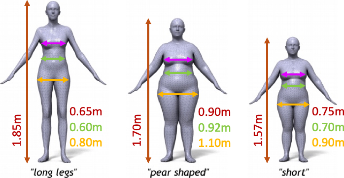
Figure 3: We crowd-source scores for linguistic body-shape attributes [Streuber:SIGGRAPH:2016] and compute anthropometric measurements for CAESAR [CAESAR] body meshes. We also crowd-source linguistic shape attribute scores for model images, like those in Fig. 2

We exploit these new datasets to train SHAPY with three novel losses, which can be exploited by any 3D human body reconstruction method: (1) We define functions of the SMPL body mesh that return a sparse set of anthropometric measurements. When measurements are available for an image we use a loss that penalizes mesh measurements that differ from the ground-truth (GT). (2) We learn a “Shape to Attribute” (S2A) function that maps 3D bodies to linguistic attribute scores. During training, we map meshes to attribute scores and penalize differences from the GT scores. (3) We similarly learn a function that maps “Attributes to Shape” (A2S). We then penalize body shape parameters that deviate from the prediction.

We study each term in detail to arrive at the final method. Evaluation is challenging because existing benchmarks with GT shape either contain too few subjects [vonMarcard2018] or have limited clothing complexity and only pseudo-GT shape [sengupta2020straps]. We fill this gap with a new dataset, named “Human Bodies in the Wild” (HBW), that contains a ground-truth 3D body scan and several in-the-wild photos of 35 subjects, for a total of 2543 photos. Evaluation on this shows that SHAPY estimates much more accurate 3D shape.

Models, data and code are available at shapy.is.tue.mpg.de.

2 Related Work

3D human pose and shape (HPS): Methods that reconstruct 3D human bodies from one or more RGB images can be split into two broad categories: (1) parametric methods that predict parameters of a statistical 3D body model, such as SCAPE [anguelov2005scape], SMPL [SMPL:2015], SMPL-X [Pavlakos2019_smplifyx], Adam [Joo2018_adam], GHUM [xu2020ghum], and (2) non-parametric methods that predict a free-form representation of the human body [varol2018bodynet, saito2020pifuhd, Jafarian_2021_CVPR, xiu2022icon]. Parametric approaches lack details w.r.t. non-parametric ones, e.g., clothing or hair. However, parametric models  disentangle the effects of identity and pose on the overall shape. Therefore, their parameters provide control for re-shaping and re-posing. Moreover, pose can be factored out to bring meshes in a canonical pose; this is important for evaluating estimates of an individual’s shape. Finally, since topology is fixed, meshes can be compared easily. For these reasons, we use a SMPL-X body model.

Parametric methods follow two main paradigms, and are based on optimization or regression. Optimization-based methods [balan2007detailed, bogo2016keep, guan_iccv_scape_2009, Pavlakos2019_smplifyx] search for model configurations that best explain image evidence, usually 2D landmarks [OpenPose_PAMI], subject to model priors that usually encourage parameters to be close to the mean of the model space. Numerous methods penalize the discrepancy between the projected and ground-truth silhouettes [MuVS_3DV_2017, lassner2017unite] to estimate shape. However, this needs special care to handle clothing [Balan:ECCV]; without this, erroneous solutions emerge that “inflate” body shape to explain the “clothed” silhouette. Regression-based methods [Choutas2020_expose, georgakis2020hierarchical, jiang2020multiperson, Kanazawa2018_hmr, Kolotouros2019_spin, Liang_2019_ICCV, VIBE:CVPR:2020, mueller2021tuch, zanfir2020weakly] are currently based on deep neural networks that directly regress model parameters from image pixels. Their training sets are a mixture of data captured in laboratory settings [ionescu2013human36m, sigal_ijcv_10b], with model parameters estimated from MoCap markers [AMASS:ICCV:2019], and in-the-wild image collections, such as COCO [lin2014coco], that contain 2D keypoint annotations. Optimization and regression can be combined, for example via in-the-network model fitting [Kolotouros2019_spin, mueller2021tuch].

Estimating 3D body shape: State-of-the-art methods are effective for estimating 3D pose, but struggle with estimating body shape under clothing. There are several reasons for this. First, 2D keypoints alone are not sufficient to fully constrain 3D body shape. Second, shape priors address the lack of constraints, but bias solutions towards “average” shapes [bogo2016keep, Pavlakos2019_smplifyx, Kolotouros2019_spin, mueller2021tuch]. Third, datasets with in-the-wild images have noisy 3D bodies, recovered by fitting a model to 2D keypoints [bogo2016keep, Pavlakos2019_smplifyx]. Fourth, datasets captured in laboratory settings have a small number of subjects, who do not represent the full spectrum of body shapes. Thus, there is a scarcity of images with known, accurate, 3D body shape. Existing methods deal with this in two ways.

First, rendering synthetic images is attractive since it gives automatic and precise ground-truth annotation. This involves shaping, posing, dressing and texturing a 3D body model [Hoffmann:GCPR:2019, sengupta2020straps, sengupta2021probabilisticCVPR, varol17_surreal, weitz2021infiniteform], then lighting it and rendering it in a scene. Doing this realistically and with natural clothing is expensive, hence, current datasets suffer from a domain gap. Alternative methods use artist-curated 3D scans [saito2019pifu, saito2020pifuhd, patel2020agora], which are realistic but limited in variety.

Second, 2D shape cues for in-the-wild images, (body-part segmentation masks [omran2018neural, Ruegg:AAAI:2020, sai2021dsr], silhouettes [agarwal_trigs_3d_poses, MuVS_3DV_2017, pavlakos2018learning]) are attractive, as these can be manually annotated or automatically detected [gong2019graphonomy, He2020maskRCNN]. However, fitting to such cues often gives unrealistic body shapes, by inflating the body to “explain” the clothing “baked” into silhouettes and masks.

Most related to our work is the work of Sengupta et al. [sengupta2020straps, sengupta2021probabilisticCVPR, sengupta2021hierarchicalICCV] who estimate body shape using a probabilistic learning approach, trained on edge-filtered synthetic images. They evaluate on the SSP-3D dataset of real images with pseudo-GT 3D bodies, estimated by fitting SMPL to multiple video frames. SSP-3D is biased to people with tight-fitting clothing. Their silhouette-based method works well on SSP-3D but does not generalize to people in normal clothing, tending to over-estimate body shape; see Fig. 1.

In contrast to previous work, SHAPY is trained with in-the-wild images paired with linguistic shape attributes, which are annotations that can be easily crowd-sourced for weak shape supervision. We also go beyond SSP-3D to provide HBW, a new dataset with in-the-wild images, varied clothing, and precise GT from 3D scans.

Shape, measurements and attributes: Body shapes can be generated from anthropometric measurements [allen2003space, seo2003synthesizing, seo2003automatic]. Tsoli et al. [tsoliWACV14] register a body model to multiple high-resolution body scans to extract body measurements. The “Virtual Caliper” [pujades2019virtual] allows users to build metrically accurate avatars of themselves using measurements or VR game controllers. ViBE [hsiao2020vibe] collects images, measurements (bust, waist, hip circumference, height) and the dress-size of models from clothing websites to train a clothing recommendation network. We draw inspiration from these approaches for data collection and supervision.

Streuber et al. [Streuber:SIGGRAPH:2016] learn BodyTalk, a model that generates 3D body shapes from linguistic attributes. For this, they select attributes that describe human shape and ask annotators to rate how much each attribute applies to a body. They fit a linear model that maps attribute ratings to SMPL shape parameters. Inspired by this, we collect attribute ratings for CAESAR meshes [CAESAR] and in-the-wild data as proxy shape supervision to train a HPS regressor. Unlike BodyTalk, SHAPY automatically infers shape from images.

Anthropometry from images: Single-View metrology [criminisi2000single] estimates the height of a person in an image, using horizontal and vertical vanishing points and the height of a reference object. Günel et al. [gunel2019face] introduce the IMDB-23K dataset by gathering publicly available celebrity images and their height information. Zhu et al. [SingleViewMetrology] use this dataset to learn to predict the height of people in images. Dey et al. [Ratan2014] estimate the height of users in a photo collection by computing height differences between people in an image, creating a graph that links people across photos, and solving a maximum likelihood estimation problem. Bieler et al. [Bieler_2019_ICCV] use gravity as a prior to convert pixel measurements extracted from a video to metric height. These methods do not address body shape.

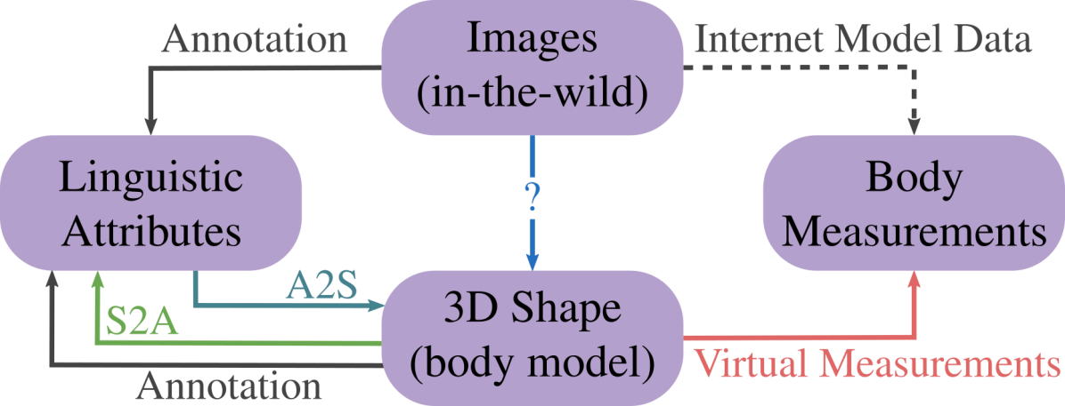
Figure 4: Shape representations and data collection. Our goal is 3D body shape estimation from in-the-wild images. Collecting data for direct supervision is difficult and does not scale. We explore two alternatives. Linguistic Shape Attributes: We annotate attributes (“A”) for CAESAR meshes, for which we have accurate shape (“S”) parameters, and learn the “A2S” and “S2A” models, to map between these representations. Attribute annotations for images can be easily crowd-sourced, making these scalable. Anthropometric Measurements: We collect images with sparse body measurements from model-agency websites. A virtual measurement module [pujades2019virtual] computes the measurements from 3D meshes. Training: We combine these sources to learn a regressor with weak supervision that infers 3D shape from an image.

3 Representations & Data for Body Shape

We use linguistic shape attributes and anthropometric measurements as a connecting component between in-the-wild images and ground-truth body shapes; see Fig. 4. To that end, we annotate linguistic shape attributes for 3D meshes and in-the-wild images, the latter from fashion-model agencies, labeled via Amazon Mechanical Turk.

3.1 SMPL-X Body Model

We use SMPL-X [Pavlakos2019_smplifyx], a differentiable model that maps shape, $\bm{\beta}$, pose, $\bm{\theta}$, and expression, $\bm{\psi}$, parameters to a 3D mesh, $M$, with $N=10,475$ vertices, $V$. The shape vector $\bm{\beta}\in\mathbb{R}^{B}$ ($B\leq 300$) has coefficients of a low-dimensional PCA space. The vertices are posed with linear blend skinning with a learned rigged skeleton, $X\in\mathbb{R}^{55\times 3}$.

3.2 Model-Agency Images

Model agencies typically provide multiple color images of each model, in various poses, outfits, hairstyles, scenes, and with a varying camera framing, together with anthropometric measurements and clothing size. We collect training data from multiple model-agency websites, focusing on under-represented body types, namely: curve-models.com, cocainemodels.com, nemesismodels.com, jayjay-models.de, kultmodels.com, modelwerk.de, models1.co.uk. showcast.de, the-models.de, and ullamodels.com. In addition to photos, we store gender and four anthropometric measurements, i.e. height, chest, waist and hip circumference, when available. To avoid having the same subject in both the training and test set, we match model identities across websites to identify models that work for several agencies. For details, see Sup. Mat.

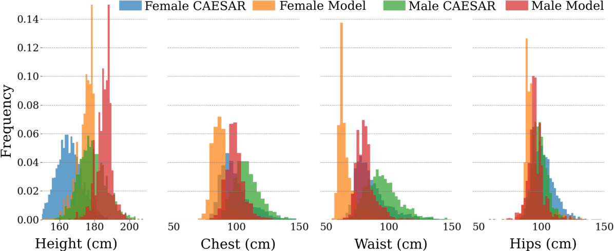
Figure 5: Histogram of height and chest/waist/hips circumference for data from model-agency websites (Sec. 3.2) and CAESAR. Model-agency data is diverse, yet not as much as CAESAR data.

After identity filtering, we have $94,620$ images of $4,419$ models along with their anthropometric measurements. However, the distributions of these measurements, shown in Fig. 5, reveal a bias for “fashion model” body shapes, while other body types are under-represented in comparison to CAESAR [CAESAR]. To enhance diversity in body-shapes and avoid strong biases and log tails, we compute the quantized 2D-distribution for height and weight and sample up to $3$ models per bin. This results in $N=1,185$ models ($714$ females, $471$ males) and $20,635$ images.

3.3 Linguistic Shape Attributes

Human body shape can be described by linguistic shape attributes [hill2015exploring]. We draw inspiration from Streuber et al. [Streuber:SIGGRAPH:2016] who collect scores for $30$ linguistic attributes for $256$ 3D body meshes, generated by sampling SMPL’s shape space, to train a linear “attribute to shape” regressor. In contrast, we train a model that takes as input an image, instead of attributes, and outputs an accurate 3D shape (and pose).

We crowd-source linguistic attribute scores for a variety of body shapes, using images from the following sources:

Rendered CAESAR images: We use CAESAR [CAESAR] bodies to learn mappings between linguistic shape attributes, anthropometric measurements, and SMPL-X shape parameters, $\bm{\beta}$. Specifically, we register a “gendered” SMPL-X model with $100$ shape components to $1,700$ male and $2,102$ female 3D scans, pose all meshes in an A-pose, and render synthetic images with the same virtual camera.

Model-agency photos: Each annotator is shown $3$ body images per subject, sampled from the image pool of Sec. 3.2.

Annotation: To keep annotation tractable, we use $A=15$ linguistic shape attributes per gender (subset of BodyTalk’s [Streuber:SIGGRAPH:2016] attributes); see Tab. 1. Each image is annotated by $K=15$ annotators on Amazon Mechanical Turk. Their task is to “indicate how strongly [they] agree or disagree that the [listed] words describe the shape of the [depicted] person’s body”; for an example, see Sup. Mat. Annotations range on a discrete 5-level Likert scale from 1 (strongly disagree) to 5 (strongly agree). We get a rating matrix $\mathbf{A}\in\{1,2,3,4,5\}^{N\times A\times K}$, where $N$ is the number of subjects. In the following, $a_{ijk}$ denotes an element of $\mathbf{A}$.

Male & Female		Male only	Female only
short	long neck	skinny arms	pear shaped
big	long legs	average	petite
tall	long torso	rectangular	slim waist
muscular	short arms	delicate build	large breasts
	broad shoulders	soft body	skinny legs
		masculine	feminine

Table 1: Linguistic shape attributes for human bodies. Some attributes apply to both genders, but others are gender specific.

4 Mapping Shape Representations

In Sec. 3 we introduce three body-shape representations: (1) SMPL-X’s PCA shape space (Sec. 3.1), (2) anthropometric measurements (Sec. 3.2), and (3) linguistic shape attribute scores (Sec. 3.3). Here we learn mappings between these, so that in Sec. 5 we can define new losses for training body shape regressors using multiple data sources.

4.1 Virtual Measurements (VM)

We obtain anthropometric measurements from a 3D body mesh in a T-pose, namely height, $0pt(\bm{\beta})$, weight, $W(\bm{\beta})$, and chest, waist and hip circumferences, $C_{\text{c}}(\bm{\beta})$, $C_{\text{w}}(\bm{\beta})$, and $C_{\text{h}}(\bm{\beta})$, respectively, by following Wuhrer et al. [wuhrer2013estimating] and the “Virtual Caliper” [pujades2019virtual]. For details on how we compute these measurements, see Sup. Mat.

4.2 Attributes and 3D Shape

Attributes to Shape (A2S): We predict SMPL-X shape coefficients from linguistic attribute scores with a second-degree polynomial regression model. For each shape $\bm{\beta}_{i}$, $i=1\dots\color[rgb]{0,0,0}N$, we create a feature vector, $\mathbf{x}_{i}^{\text{\mbox{A2S}}}$, by averaging for each of the $A$ attributes the corresponding $K$ scores:

$${\color[rgb]{0,0,0}{{\color[rgb]{0,0,0}{\color[rgb]{0,0,0}\mathbf{x}}_{i}^{\text{\mbox{A2S}}}}=[\bar{a}_{i,1},\dots,\bar{a}_{i,A}]\text{,}\quad\quad\bar{a}_{i,j}=\frac{1}{K}\sum_{k=1}^{K}a_{ijk}\text{,}}}$$ (1)

where $i$ is the shape index (list of “fashion” or CAESAR bodies), $j$ is the attribute index, and $k$ the annotation index.

We then define the full feature matrix for all $N$ shapes as:

$${\color[rgb]{0,0,0}{\mathbf{X}^{\text{\mbox{A2S}}}}}=[\phi({\color[rgb]{0,0,0}\mathbf{x}}_{1}^{\text{\mbox{A2S}}}),\quad\dots,\quad\phi({\color[rgb]{0,0,0}\mathbf{x}}_{N}^{\text{\mbox{A2S}}})]^{\top}\text{,}$$ (2)

where $\phi(\mathbf{x}_{i}^{\text{\mbox{A2S}}})$ maps $\mathbf{x}_{i}$ to 2^nd order polynomial features.

The target matrix $\mathbf{Y}=[\bm{\beta}_{1},\dots,\bm{\beta}_{N}]^{\top}$ contains the shape parameters $\bm{\bm{\beta}}_{i}=[\bm{\beta}_{i,1},\dots,\bm{\beta}_{i,B}]^{\top}$. We compute the polynomial model’s coefficients $\bm{W}$ via least-squares fitting:

$$\mathbf{Y}=\mathbf{XW}+\epsilon\text{.}$$ (3)

Empirically, the polynomial model performs better than several models that we evaluated; for details, see Sup. Mat.

Shape to Attributes (S2A): We predict linguistic attribute scores, $A$, from SMPL-X shape parameters, $\bm{\beta}$. Again, we fit a second-degree polynomial regression model. S2A has “swapped” inputs and outputs w.r.t. A2S:

$$\mathbf{x}_{i}^{\text{\mbox{S2A}}} =[\bm{\beta}_{i,1},\dots,\bm{\beta}_{i,B}]\text{,}$$ (4)

$$\mathbf{y}_{i} ={\color[rgb]{0,0,0}{[\bar{a}_{i,1},\dots,\bar{a}_{i,A}]^{\top}}}\text{.}$$ (5)

Attributes & Measurements to Shape (AHWC2S): Given a sparse set of anthropometric measurements, we predict SMPL-X shape parameters, $\bm{\beta}$. The input vector is:

$$\mathbf{x}_{i}^{\text{\mbox{{\color[rgb]{0.76,0.01,0}{H}}{\color[rgb]{1,0.39,0.13}{W}}{\color[rgb]{1,0,0.5}{C}}2S}}}=[{\color[rgb]{0.76,0.01,0}{h_{i}}},{\color[rgb]{1,0.39,0.13}{w_{i}}},{\color[rgb]{1,0,0.5}{c_{c_{i}},c_{w_{i}},c_{h_{i}}}}]\text{,}$$ (6)

where $c_{c},c_{w},c_{h}$ is the chest, waist, and hip circumference, respectively, $h$ and $w$ are the height and weight, and HWC2S means Height + Weight + Circumference to Shape. The regression target is the SMPL-X shape parameters, $\mathbf{y}_{i}$.

When both Attributes and measurements are available, we combine them for the AHWC2S model with input:

$$\mathbf{x}_{i}^{\text{\mbox{{\color[rgb]{0,0.75,0.16}{A}}{\color[rgb]{0.76,0.01,0}{H}}{\color[rgb]{1,0.39,0.13}{W}}{\color[rgb]{1,0,0.5}{C}}2S}}}=[{\color[rgb]{0,0.75,0.16}{\bar{a}_{i,1},\dots,\bar{a}_{i,A}}},{\color[rgb]{0.76,0.01,0}{h_{i}}},{\color[rgb]{1,0.39,0.13}{w_{i}}},{\color[rgb]{1,0,0.5}{c_{c_{i}},c_{w_{i}},c_{h_{i}}}}]\text{.}$$ (7)

In practice, depending on which measurements are available, we train and use different regressors. Following the naming convention of AHWC2S, these models are: AH2S, AHW2S, AC2S, and AHC2S, as well as their equivalents without attribute input H2S, HW2S, C2S, and HC2S. For an evaluation of the contribution of linguistic shape attributes on top of each anthropometric measurement, see Sup. Mat.

Training Data: To train the A2S and S2A mappings we use CAESAR data, for which we have SMPL-X shape parameters, anthropometric measurements, and linguistic attribute scores. We train separate gender-specific models.

5 3D Shape Regression from an Image

We present SHAPY, a network that predicts SMPL-X parameters from an RGB image with more accurate body shape than existing methods. To improve the realism and accuracy of shape, we explore training losses based on all shape representations discussed above, i.e., SMPL-X meshes (Sec. 3.1), linguistic attribute scores (Sec. 3.3) and anthropometric measurements (Sec. 4.1). In the following, symbols with/-out a hat are regressed/ground-truth values.

We convert shape $\hat{\bm{\beta}}$ to height and circumferences values $\{\hat{0}pt,\hat{C}_{\text{c}},\hat{C}_{\text{w}},\hat{C}_{\text{h}}\}=$ $\{0pt(\hat{\bm{\beta}}),C_{\text{c}}(\hat{\bm{\beta}}),C_{\text{w}}(\hat{\bm{\beta}}),C_{\text{h}}(\hat{\bm{\beta}})\}$, by applying our virtual measurement tool (Sec. 4.1) to the mesh $M(\hat{\bm{\beta}})$ in the canonical T-pose. We also convert shape $\hat{\bm{\beta}}$ to linguistic attribute scores, with $\hat{A}=\text{\text{\mbox{S2A}}}(\hat{\bm{\beta}})$.

We train various SHAPY versions with the following “SHAPY losses”, using either linguistic shape attributes, or anthropometric measurements, or both:

$$L_{\text{{\color[rgb]{0,0.75,0.16}{attr}}}} =||A-\hat{A}||_{2}^{2}\text{,}$$ (8)

$$L_{\text{{\color[rgb]{0.76,0.01,0}{height}}}} =||0pt-\hat{H}||_{2}^{2}\text{,}$$ (9)

$$L_{\text{{\color[rgb]{1,0,0.5}{circ}}}} =\sum\nolimits_{i\in\{c,w,h\}}||C_{i}-\hat{C}_{i}||^{2}_{2}$$ (10)

These are optionally added to a base loss, $L_{\text{\mbox{base}}}$, defined below in “training details”. The architecture of SHAPY, with all optional components, is shown in Fig. 6. A suffix of color-coded letters describes which of the above losses are used when training a model. For example, SHAPY-AH denotes a model trained with the attribute and height losses, i.e.: $L_{\text{{\color[rgb]{0,0,0}SHAPY}-\text{\mbox{{\color[rgb]{0,0.75,0.16}{A}}{\color[rgb]{0.76,0.01,0}{H}}2S}}}}=L_{\text{\mbox{base}}}+L_{\text{{\color[rgb]{0,0.75,0.16}{attr}}}}+L_{\text{{\color[rgb]{0.76,0.01,0}{height}}}}$.

Figure 6: SHAPY first estimates shape, $\hat{\beta}$, and pose, $\hat{\theta}$. Shape is used by: (1) our virtual anthropometric measurement (VM) module to compute height, $\hat{H}$, and circumferences, $\hat{C}$, and (2) our S2A module to infer linguistic attribute scores, $\hat{A}$. There are several SHAPY variations, e.g., SHAPY-H uses only VM to infer $\hat{H}$, while SHAPY-HA uses VM to infer $\hat{H}$ and S2A to infer $\hat{A}$.

Training Details: We initialize SHAPY with the ExPose [Choutas2020_expose] network weights and use curated fits [Choutas2020_expose], H3.6M [ionescu2013human36m], the SPIN [Kolotouros2019_spin] training data, and our model-agency dataset (Sec. 3.2) for training. In each batch, 50% of the images are sampled from the model-agency images, for which we ensure a gender balance. The “SHAPY losses” of Eqs. 8, 9 and 10 are applied only on the model-agency images. We use these on top of a standard base loss:

$$L_{\text{\mbox{base}}} =L_{\text{pose}}+L_{\text{shape}}\text{,}$$ (11)

where $L_{\text{joints}}^{\text{2D}}$ and $L_{\text{joints}}^{\text{3D}}$ are 2D and 3D joint losses:

$$L_{\text{pose}} =L_{\text{joints}}^{\text{2D}}+L_{\text{joints}}^{\text{3D}}+L_{\bm{\theta}}\text{,}$$ (12)

$$L_{\text{shape}} =L_{\bm{\beta}}+L_{\bm{\beta}}^{\text{prior}}\text{,}$$ (13)

$L_{\bm{\theta}}$ and $L_{\bm{\beta}}$ are losses on pose and shape parameters, and $L_{\bm{\beta}}^{\text{prior}}$ is PIXIE’s [feng2021pixie] “gendered” shape prior. All losses are L2, unless otherwise explicitly specified. Losses on SMPL-X parameters are applied only on the pose data [ionescu2013human36m, Choutas2020_expose, Kolotouros2019_spin]. For more implementation details, see Sup. Mat.

6 Experiments

6.1 Evaluation Datasets

3D Poses in the Wild (3DPW) [vonMarcard2018]: We use this to evaluate pose accuracy. This is widely used, but has only 5 test subjects, i.e., limited shape variation. For results, see Sup. Mat.

Sports Shape and Pose 3D (SSP-3D)[sengupta2020straps]: We use this to evaluate 3D body shape accuracy from images. It has $62$ tightly-clothed subjects in $311$ in-the-wild images from Sports-1M [KarpathyCVPR14], with pseudo ground-truth SMPL meshes that we convert to SMPL-X for evaluation.

Model Measurements Test Set (MMTS): We use this to evaluate anthropometric measurement accuracy, as a proxy for body shape accuracy. To create MMTS, we withhold 2699/1514 images of 143/95 female/male identities from our model-agency data, described in Sec. 3.2

CAESAR Meshes Test Set (CMTS): We use CAESAR to measure the accuracy of SMPL-X body shapes and linguistic shape attributes for the models of Sec. 4. Specifically, we compute: (1) errors for SMPL-X meshes estimated from linguistic shape attributes and/or anthropometric measurements by A2S and its variations, and (2) errors for linguistic shape attributes estimated from SMPL-X meshes by S2A. To create an unseen mesh test set, we withhold 339 male and 410 female CAESAR meshes from the crowd-sourced CAESAR  linguistic shape attributes, described in Sec. 3.3.

Human Bodies in the Wild (HBW): The field is missing a dataset with varied bodies, varied clothing, in-the-wild images, and accurate 3D shape ground truth. We fill this gap by collecting a novel dataset, called “Human Bodies in the Wild” (HBW), with three steps: (1) We collect accurate 3D body scans for 35 subjects (20 female, 15 male), and register a “gendered” SMPL-X model to these to recover 3D SMPL-X ground-truth bodies [Dyna]. (2) We take photos of each subject in “photo-lab” settings, i.e., in front of a white background with controlled lighting, and in various everyday outfits and “fashion” poses. (3) Subjects upload full-body photos of themselves taken in the wild. For each subject we take up to 111 photos in lab settings, and collect up to 126 in-the-wild photos. In total, HBW has 2543 photos, 1,318 in the lab setting and 1,225 in the wild. We split the data into a validation and a test set (val/test) with 10/25 subjects (6/14 female 4/11 male) and 781/1,762 images (432/983 female 349/779 male), respectively. Figure 7 shows a few HBW subjects, photos and their SMPL-X ground-truth shapes. All subjects gave prior written informed consent to participate in this study and to release the data. The study was reviewed by the ethics board of the University of Tübingen, without objections.

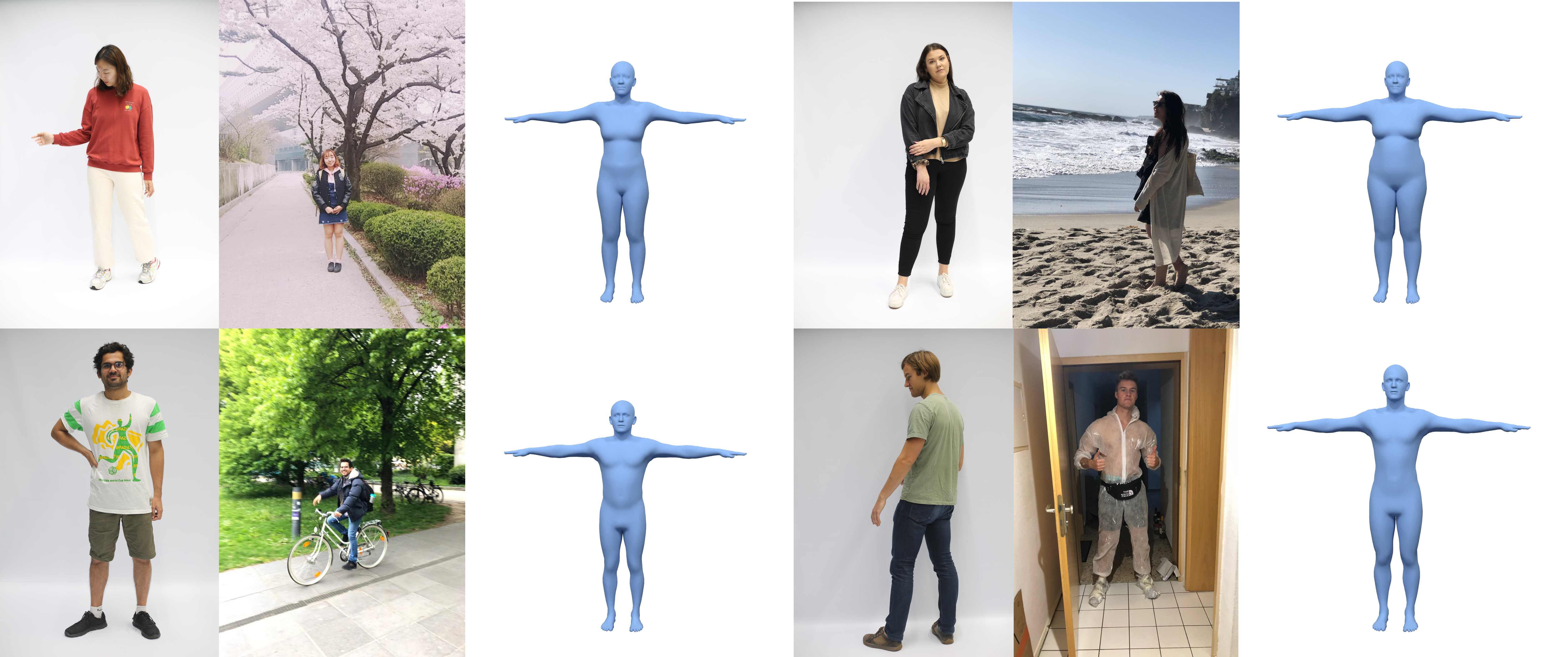
Figure 7: “Human Bodies in the Wild” (HBW) color images, taken in the lab and in the wild, and the SMPL-X ground-truth shape.

6.2 Evaluation Metrics

We use standard accuracy metrics for 3D body pose, but also introduce metrics specific to 3D body shape.

Anthropometric Measurements: We report the mean absolute error in mm between ground-truth and estimated measurements, computed as described in Sec. 4.1. When weight is available, we report the mean absolute error in kg.

MPJPE and V2V metrics: We report in Sup. Mat. the mean per-joint point error (MPJPE) and mean vertex-to-vertex error (V2V), when SMPL-X meshes are available. The prefix “PA” denotes metrics after Procrustes alignment.

Mean point-to-point error ($\text{P2P}_{20\text{K}}$): SMPL-X has a highly non-uniform vertex distribution across the body, which negatively biases the mean vertex-to-vertex (V2V) error, when comparing estimated and ground-truth SMPL-X meshes. To account for this, we evenly sample $20$K points on SMPL-X’s surface, and report the mean point-to-point ($\text{P2P}_{20\text{K}}$) error. For details, see Sup. Mat.

6.3 Shape-Representation Mappings

We evaluate the models A2S and S2A, which map between the various body shape representations (Sec. 4).

	Method	$\text{P2P}_{20\text{K}}$	Height	Weight	Chest	Waist	Hips
	-	(mm)	(mm)	(kg)	(mm)	(mm)	(mm)
Male subjects	A2S	$11.1\pm 5.2$	$29\pm 21$	$5\pm 4$	$30\pm 22$	$32\pm 24$	$28\pm 21$
	H2S	$12.1\pm 6.1$	$5\pm 4$	$11\pm 11$	$81\pm 66$	$102\pm 87$	$40\pm 33$
	AH2S	$6.8\pm 2.3$	$4\pm 3$	$3\pm 3$	$27\pm 21$	$29\pm 23$	$24\pm 18$
	HW2S	$8.1\pm 2.7$	$5\pm 4$	$1\pm 1$	$24\pm 17$	$26\pm 20$	$21\pm 18$
	AHW2S	$6.3\pm 2.1$	$4\pm 3$	$1\pm 1$	$19\pm 15$	$19\pm 14$	$20\pm 16$
	C2S	$19.7\pm 11.1$	$59\pm 47$	$9\pm 8$	$55\pm 41$	$63\pm 49$	$37\pm 28$
	AC2S	$9.6\pm 4.4$	$25\pm 19$	$3\pm 3$	$23\pm 19$	$21\pm 17$	$18\pm 14$
	HC2S	$7.7\pm 2.6$	$5\pm 4$	$2\pm 2$	$28\pm 23$	$18\pm 15$	$13\pm 11$
	AHC2S	$6.0\pm 2.0$	$4\pm 3$	$2\pm 2$	$21\pm 17$	$17\pm 14$	$13\pm 10$
	HWC2S	$7.3\pm 2.6$	$5\pm 4$	$1\pm 1$	$20\pm 15$	$14\pm 12$	$13\pm 11$
	AHWC2S	$5.8\pm 2.0$	$4\pm 3$	$1\pm 1$	$16\pm 13$	$13\pm 10$	$13\pm 10$

Table 2: Results of A2S variants on CMTS for male subjects, using the male SMPL-X model. For females, see Sup. Mat.

A2S and its variations: How well can we infer 3D body shape from just linguistic shape attributes, anthropometric measurements, or both of these together? In Tab. 2, we report reconstruction and measurement errors using many combinations of attributes (A), height (H), weight (W), and circumferences (C). Evaluation on CMTS data shows that attributes improve the overall shape prediction across the board. For example, height+attributes (AH2S) has a lower point-to-point error than height alone. The best performing model, AHWC, uses everything, with $\text{P2P}_{20\text{K}}$-errors of $5.8\pm 2.0$ mm (males) and $6.2\pm 2.4$ mm (females).

S2A: How well can we infer linguistic shape attributes from 3D shape? S2A’s accuracy on inferring the attribute Likert score is $75\%/69\%$ for males/females; details in Sup. Mat.

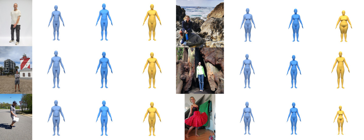
Figure 8: Qualitative results from HBW. From left to right: RGB, ground-truth shape, SHAPY and Sengupta et al. [sengupta2021hierarchicalICCV]. For example, in the upper- and lower- right images, SHAPY is less affected by pose variation and loose clothing.

6.4 3D Shape from an Image

We evaluate all of our model’s variations (see Sec. 5) on the HBW validation set and find, perhaps surprisingly, that SHAPY-A outperforms other variants. We refer to this below (and Fig. 1) simply as “SHAPY” and report its performance in Tab. 3 for HBW, Tab. 4 for MMTS, and Tab. 5 for SSP-3D. For images with natural and varied clothing (HBW, MMTS), SHAPY significantly outperforms all other methods (Tabs. 3 and 4) using only weak 3D shape supervision (Attributes). On these images, Sengupta et al.’s method [sengupta2021hierarchicalICCV] struggles with the natural clothing. In contrast, their method is more accurate than SHAPY on SSP-3D (Tab. 5), which has tight “sports” clothing, in terms of PVE-T-SC, a scale-normalized metric used on this dataset. These results show that silhouettes are good for tight/minimal clothing and that SHAPY struggles with high BMI shapes due to the lack of such shapes in our training data; see Fig. 5. Note that, as HBW has true ground-truth 3D shape, it does not need SSP-3D’s scaling for evaluation.

Method	Model	Height	Chest	Waist	Hips	$\text{P2P}_{20\text{K}}$
SMPLR [madadi2020smplr]	SMPL	182	267	309	305	69
STRAPS [sengupta2020straps]	SMPL	135	167	145	102	47
SPIN [Kolotouros2019_spin]	SMPL	59	92	78	101	29
TUCH [mueller2021tuch]	SMPL	58	89	75	57	26
Sengupta et al. [sengupta2021hierarchicalICCV]	SMPL	82	133	107	63	32
ExPose [Choutas2020_expose]	SMPL-X	85	99	92	94	35
SHAPY (ours)	SMPL-X	51	65	69	57	21

Table 3: Evaluation on the HBW test set in mm. We compute the measurement and point-to-point ($\text{P2P}_{20\text{K}}$) error between predicted and ground-truth SMPL-X meshes.

	Mean absolute error (mm) $\downarrow$
Method	Model	Height	Chest	Waist	Hips
Sengupta et al. [sengupta2021hierarchicalICCV]	SMPL	84	186	263	142
TUCH [mueller2021tuch]	SMPL	82	92	129	91
SPIN [Kolotouros2019_spin]	SMPL	72	91	129	101
STRAPS [sengupta2020straps]	SMPL	207	278	326	145
ExPose [Choutas2020_expose]	SMPL-X	107	107	136	92
SHAPY (ours)	SMPL-X	71	64	98	74

Table 4: Evaluation on MMTS. We report the mean absolute error between ground-truth and estimated measurements.

A key observation is that training with linguistic shape attributes alone is sufficient, i.e., without anthropometric measurements. Importantly, this opens up the possibility for significantly larger data collections. For a study of how different measurements or attributes impact accuracy, see Sup. Mat. Figure 8 shows SHAPY’s qualitative results.

7 Conclusion

SHAPY is trained to regress more accurate human body shape from images than previous methods, without explicit 3D shape supervision. To achieve this, we present two different ways to collect proxy annotations for 3D body shape for in-the-wild images. First, we collect sparse anthropometric measurements from online model-agency data. Second, we annotate images with linguistic shape attributes using crowd-sourcing. We learn mappings between body shape, measurements, and attributes, enabling us to supervise a regressor using any combination of these. To evaluate SHAPY, we introduce a new shape estimation benchmark, the “Human Bodies in the Wild” (HBW) dataset. HBW has images of people in natural clothing and natural settings together with ground-truth 3D shape from a body scanner. HBW is more challenging than existing shape benchmarks like SSP-3D, and SHAPY significantly outperforms existing methods on this benchmark. We believe this work will open new directions, since the idea of leveraging linguistic annotations to improve 3D shape has many applications.

Method	Model	PVE-T-SC	mIOU
HMR [Kanazawa2018_hmr]	SMPL	22.9	0.69
SPIN [Kolotouros2019_spin]	SMPL	22.2	0.70
STRAPS [sengupta2020straps]	SMPL	15.9	0.80
Sengupta et al. [sengupta2021hierarchicalICCV]	SMPL	13.6	-
SHAPY (ours)	SMPL-X	19.2	-

Table 5: Evaluation on the SSP-3D test set [sengupta2020straps]. We report the scaled mean vertex-to-vertex error in T-pose [sengupta2020straps], and mIOU.

Limitations: Our model-agency training dataset (Sec. 3.2) is not representative of the entire human population and this limits SHAPY’s ability to predict larger body shapes. To address this, we need to find images of more diverse bodies together with anthropometric measurements and linguistic shape attributes describing them.

Social impact: Knowing the 3D shape of a person has advantages, for example, in the clothing industry to avoid unnecessary returns. If used without consent, 3D shape estimation may invade individuals’ privacy. As with all other 3D pose and shape estimation methods, surveillance and deep-fake creation is another important risk. Consequently, SHAPY’s license prohibits such uses.

Acknowledgments: This work was supported by the Max Planck ETH Center for Learning Systems and the International Max Planck Research School for Intelligent Systems. We thank Tsvetelina Alexiadis, Galina Henz, Claudia Gallatz, and Taylor McConnell for the data collection, and Markus Höschle for the camera setup. We thank Muhammed Kocabas, Nikos Athanasiou and Maria Alejandra Quiros-Ramirez for the insightful discussions.

Disclosure: https://files.is.tue.mpg.de/black/CoI_CVPR_2022.txt

Appendix A Data Collection

A.1 Model-Agency Identity Filtering

We collect internet data consisting of images and height/chest/waist/hips measurements, from model agency websites. A “fashion model” can work for many agencies and their pictures can appear on multiple websites. To create non-overlapping training, validation and test sets, we match model identities across websites. To that end, we use ArcFace [deng2018arcface] for face detection and RetinaNet [Deng_2020_CVPR] to compute identity embeddings $E_{i}\in\mathbb{R}^{512}$ for each image. For every pair of models $(q,t)$ with the same gender label, let $Q$, $T$ be the number of query and target model images and $\bm{E_{Q}}\in\mathbb{R}^{Q\times 512}$ and $\bm{E_{T}}\in\mathbb{R}^{T\times 512}$ the query and target embedding feature matrices. We then compute the pairwise cosine similarity matrix $\mathcal{S}\in\mathbb{R}^{Q\times T}$ between all images in $\bm{E_{Q}}$ and $\bm{E_{T}}$, and the aggregate and average similarity:

$$\mathcal{S}_{T}(t) =\frac{1}{Q}\sum_{q}\mathcal{S}(q,t),$$ (14)

$$\mathcal{S}_{TQ} =\frac{1}{QT}\sum_{q}\sum_{t}\mathcal{S}(q,t).$$ (15)

Each pair with $\mathcal{S}$ and $\mathcal{S}_{T}$ that has no element larger than the similarity threshold $\tau=0.3$ is ignored, as it contains dissimilar models. Finally, we check if $\mathcal{S}_{TQ}$ is larger than $\tau$, and we keep a list of all pairs for which this holds true.

A.2 Crowd-Sourced Linguistic Shape-Attributes

To collect human ratings of how much a word describes a body shape, we conduct a human intelligence task (HIT) on Amazon Mechanical Turk (AMT). In this task, we show an image of a person along with $15$ different gender-specific attributes. We then ask participants to indicate how strongly they agree or disagree that the provided words describe the shape of this person’s body. We arrange the rating buttons from strong disagreement to strong agreement with equal distances to create a $5$-point Likert scale. The rating choices are “strongly disagree” (score $1$), “rather disagree” (score $2$), “average” (score $3$), “rather agree” (score $4$), “strongly agree” (score $5$).

We ask multiple persons to rate each body and image, to “average out” the subjectivity of individual ratings [Streuber:SIGGRAPH:2016]. Additionally, we compute the Pearson correlation between averaged attribute ratings and ground-truth measurements. Examples of highly correlated pairs are “Big / Weight”, and “Short / Height”.

The layout of our CAESAR annotation task is visualized in Fig. A.1. To ensure good rating quality, we have several qualification requirements per participant: submitting a minimum of $5000$ tasks on AMT and an AMT acceptance rate of $95\%$, as well as having a US residency and passing a language qualification test to ensure similar language skills and cultures across raters.

Figure A.1: Layout of the AMT task for a male subject. Left: the 3D body mesh in A-pose. Right: the attributes and ratings buttons.

Appendix B Mapping Shape Representations

B.1 Shape to Anatomical Measurements (S2M)

An important part of our project is the computation of body measurements. Following “Virtual Caliper” [pujades2019virtual], we present a method to compute anatomical measurements from a 3D mesh in the canonical T-pose, i.e. after “undoing” the effect of pose. Specifically, we measure the height, $0pt(\bm{\beta})$, weight, $W(\bm{\beta})$, and the chest, waist and hip circumferences, $C_{\text{c}}(\bm{\beta})$, $C_{\text{w}}(\bm{\beta})$, and $C_{\text{h}}(\bm{\beta})$, respectively. Let $v_{\text{head}}(\bm{\beta}),v_{\text{left heel}}(\bm{\beta}),v_{\text{chest}}(\bm{\beta}),v_{\text{waist}}(\bm{\beta}),v_{\text{hip}}(\bm{\beta})$ be the head, left heel, chest, waist and hip vertices. $0pt(\bm{\beta})$ is computed as the difference in the vertical-axis “Y” coordinates between the top of the head and the left heel: $0pt(\bm{\beta})=\lvert v_{\text{head}}^{y}(\bm{\beta})-v_{\text{left heel}}^{y}(\bm{\beta})\rvert$ . To obtain $W(\bm{\beta})$ we multiply the mesh volume by 985 kg/m³, which is the average human body density. We compute circumference measurements using the method of Wuhrer et al. [wuhrer2013estimating].

Here, $T\in\mathbb{R}^{F\times 3\times 3}$ , where $F=20,908$ is the number of triangles in the SMPL-X mesh, denotes “shaped” vertices of all triangles of the mesh $M(\bm{\beta},\bm{\theta})$ ; we drop expressions, $\bm{\psi}$, which are not used in this work. Let us explain this using the chest circumference $C_{\text{c}}(\bm{\beta})$ as an example. We form a plane $P$ with normal $\bm{n}=(0,1,0)$ that crosses the point $v_{\text{chest}}(\bm{\beta})$. Then, let $\mathcal{I}=\{\bm{p}_{i}\}_{i=1}^{N}$ be the set of points of $P$ that intersect the body mesh (red points in Fig. A.2). We store their barycentric coordinates $(\mathtt{u}_{i},\mathtt{v}_{i},\mathtt{w}_{i})$ and the corresponding body-triangle index $t_{i}$. Let $\mathcal{H}$ be the convex hull of $\mathcal{I}$ (black lines in Fig. A.2), and $\mathcal{E}$ the set of edge indices of $\mathcal{H}$. $C_{\text{c}}(\bm{\beta})$ is equal to the length of the convex hull:

$$C_{\text{c}}(\bm{\beta})=\sum_{(i,j)\in\mathcal{E}}\left\lVert\begin{pmatrix}\mathtt{u}_{i}\\ \mathtt{v}_{i}\\ \mathtt{w}_{i}\end{pmatrix}^{\top}T_{t_{i}}-\begin{pmatrix}\mathtt{u}_{j}\\ \mathtt{v}_{j}\\ \mathtt{w}_{j}\end{pmatrix}^{\top}T_{t_{j}}\right\rVert_{2},$$ (16)

where $i,j$ are point indices for line segments of $\mathcal{E}$. The process is the same for the waist and hips, but the intersection plane is computed using $v_{\text{waist}},v_{\text{hip}}$. All of $0pt(\bm{\beta}),W(\bm{\beta}),C_{\text{c}}(\bm{\beta}),C_{\text{w}}(\bm{\beta}),C_{\text{h}}(\bm{\beta})$ are differentiable functions of body shape parameters, $\bm{\beta}$.

Note that SMPL-X knows the height distribution of humans and acts as a strong prior in shape estimation. Given the ground-truth height of a person (in meter), $0pt(\bm{\beta})$ can be used to directly supervise height and overcome scale ambiguity.

Figure A.2: Automatic anatomical measurements on a 3D mesh. The red points lie on the intersection of planes at chest/waist/hip height with the mesh, while their convex hull is shown with black lines.

B.2 Mapping Attributes to Shape (A2S)

We introduce A2S, a model that maps the input attribute ratings to shape components $\bm{\beta}$ as output. We compare a $2^{\text{nd}}$ degree polynomial model with a linear regression model and a multi-layer perceptron (MLP), using the Vertex-to-Vertex (V2V) error metric between predicted and ground-truth SMPL-X meshes, and report results in Tab. A.1. When using only attributes as input (A2S), the polynomial model of degree $d=2$ achieves the best performance. Adding height and weight to the input vector requires a small modification, namely using the cubic root of the weight and converting the height from (m) to (cm). We. With these additions, the $2^{\text{nd}}$ degree polynomial achieves the best performance.

Model	Input	V2V mean $\pm$ std
		Females	Males
Mean Shape		18.01 $\pm$ 8.73	19.24 $\pm$ 10.36
Linear Regression	A	10.83 $\pm$ 4.77	10.43 $\pm$ 4.63
Polynomial (d=2)	A	10.58 $\pm$ 4.67	10.25 $\pm$ 4.48
MLP	A	10.73 $\pm$ 4.62	10.33 $\pm$ 4.57
Linear Regression	A+H+W	7.00 $\pm$ 2.59	6.56 $\pm$ 2.21
Polynomial (d=2)	A+H+W	7.31 $\pm$ 2.56	6.71 $\pm$ 2.21
MLP	A+H+W	7.03 $\pm$ 2.6	6.68 $\pm$ 2.24
Linear Regression	A+H+$\sqrt[3]{W}$	6.97 $\pm$ 2.58	6.54 $\pm$ 2.22
Polynomial (d=2)	A+H+ $\sqrt[3]{W}$	6.88 $\pm$ 2.55	6.49 $\pm$ 2.20

Table A.1: Comparison of models for A2S and AHW2S regression.

B.3 Images to Attributes (I2A)

We briefly experimented with models that learn to predict attribute scores from images (I2A). This attribute predictor is implemented using a ResNet50 for feature extraction from the input images, followed by one MLP per gender for attribute score prediction. To quantify the model’s performance, we use the attribute classification metric described in the main paper. I2A achieves $60.7$ / $69.3\%$ (fe-/male) of correctly predicted attributes, while our S2A achieves $68.8$ / $76\%$ on CAESAR. Our explanation for this result is that it is hard for the I2A model to learn to correctly predict attributes independent of subject pose. Our approach works better, because it decomposes 3D human estimation into predicting pose and shape. Networks are good at estimating pose even without GT shape [li2021hybrik]. “SHAPY ’s losses” affect only the shape branch. To minimize these losses, the network has to learn to correctly predict shape irrespective of pose variations.

Appendix C SHAPY- 3D Shape Regression from Images

Implementation details:: To train SHAPY, each batch of training images contains $50\%$ images collected from model agency websites and $50\%$ images from ExPose’s [Choutas2020_expose] training set. Note that the overall number of images of males and females in our collected model data differs significantly; images of female models are many more. Therefore, we randomly sample a subset of female images so that, eventually, we get an equal number of male and female images. We also use the BMI of each subject, when available, as a sampling weight for images. In this way, subjects with higher BMI are selected more often, due to their smaller number, to avoid biasing the model towards the average BMI of the dataset. Our pipeline is implemented in PyTorch [pytorch] and we use the Adam [adam] optimizer with a learning rate of $1e-4$. We tune the weights of each loss term with grid search on the MMTS and HBW validation sets. Using a batch size of $48$, SHAPY achieves the best performance on the HBW validation set after 80k steps.

Appendix D Experiments

D.1 Metrics

$\text{P2P}_{20\text{K}}$: SMPL-X has more than half of its vertices on the head. Consequently, computing an error based on vertices overemphasizes the importance of the head. To remove this bias, we also report the mean distance between $P=20k$ mesh surface points; see Fig. A.3 for a visualization on the ground-truth and estimated meshes. For this, we uniformly sample the SMPL-X template mesh and compute a sparse matrix $\mathbf{H}_{\text{\mbox{SMPL-X}}}\in\mathbb{R}^{P\times N}$ that regresses the mesh surface points from SMPL-X vertices $V$, as $\mathbf{P}=\mathbf{H}_{\text{\mbox{SMPL-X}}}V$.

To use this metric in a mesh with different topology, e.g. SMPL, we simply need to compute the corresponding $\mathbf{H}_{\text{\mbox{SMPL}}}$. For this, we align the SMPL model to the SMPL-X template mesh. For each point sampled from the SMPL-X mesh surface, we find the closest point on the aligned SMPL mesh surface. To obtain the SMPL mesh surface points from SMPL vertices, we again compute a sparse matrix, $\mathbf{H}_{\text{\mbox{SMPL}}}\in\mathbb{R}^{P\times 6,890}$. The distance between the SMPL-X and SMPL mesh surface points on the template meshes is $0.073$ mm, which is negligible.

Given two meshes $M_{1}$ and $M_{2}$ of topology $T_{1}$ and $T_{2}$ we obtain the mesh surface points $P_{1}=\mathbf{H}_{T_{1}}U_{1}$ and $P_{2}=\mathbf{H}_{T_{2}}U_{2}$, where $U_{1}$ and $U_{2}$ denote the vertices of the shaped zero posed (t-pose) meshes. To compute the $\text{P2P}_{20\text{K}}$ error we correct for translation $t=\bar{P}_{2}-\bar{P}_{1}$ and define

$$\mbox{$\text{P2P}_{20\text{K}}$}(U_{1},U_{2})=||\mathbf{H}_{T_{1}}U_{1}+t-\mathbf{H}_{T_{2}}U_{2}||_{2}^{2}\text{.}$$

Figure A.3: The 20K body mesh surface points (in black) used to evaluated body shape estimation accuracy.

Mean absolute error (mm) $\downarrow$
Method	Height	Chest	Waist	Hips
SHAPY-H	52	113	172	108
SHAPY-HA	60	64	96	77
SHAPY-C	119	66	70	70
SHAPY-CA	74	60	82	69
SHAPY-HC	54	62	72	69
SHAPY-HCA	57	61	85	73

Table A.2: Leave-one-out evaluation on MMTS.

Mean absolute error (mm) $\downarrow$
Method	Height	Chest	Waist	Hips	$\text{P2P}_{20\text{K}}$
SHAPY-H	54	90	77	54	22
SHAPY-HA	49	62	71	58	20
SHAPY-C	72	65	77	60	26
SHAPY-CA	54	69	78	58	22
SHAPY-HC	53	61	77	55	23
SHAPY-HCA	47	66	75	52	20

Table A.3: Leave-one-out evaluation on the HBW test set.

Attribute	Male		Female
	MAE $\pm$ SD	CCP	MAE $\pm$ SD	CCP
Big	$0.25\pm 0.18$	$71.68\%$	$0.31\pm 0.23$	$70.00\%$
Broad Shoulders	$0.26\pm 0.20$	$73.75\%$	$0.33\pm 0.24$	$63.90\%$
Long Legs	$0.23\pm 0.17$	$81.12\%$	$0.43\pm 0.33$	$58.05\%$
Long Neck	$0.27\pm 0.21$	$73.75\%$	$0.29\pm 0.21$	$69.51\%$
Long Torso	$0.27\pm 0.20$	$70.80\%$	$0.36\pm 0.27$	$62.68\%$
Muscular	$0.31\pm 0.24$	$69.03\%$	$0.26\pm 0.21$	$73.17\%$
Short	$0.28\pm 0.22$	$72.27\%$	$0.27\pm 0.21$	$67.56\%$
Short Arms	$0.20\pm 0.15$	$84.07\%$	$0.27\pm 0.22$	$72.20\%$
Tall	$0.27\pm 0.22$	$70.80\%$	$0.30\pm 0.23$	$70.98\%$
Average	$0.27\pm 0.19$	$78.76\%$	n / a	n / a
Delicate Build	$0.21\pm 0.16$	$78.17\%$	n / a	n / a
Masculine	$0.23\pm 0.18$	$78.17\%$	n / a	n / a
Rectangular	$0.27\pm 0.20$	$80.24\%$	n / a	n / a
Skinny Arms	$0.25\pm 0.19$	$76.40\%$	n / a	n / a
Soft Body	$0.32\pm 0.23$	$68.14\%$	n / a	n / a
Large Breasts	n / a	n / a	$0.31\pm 0.23$	$72.93\%$
Pear Shaped	n / a	n / a	$0.32\pm 0.22$	$64.39\%$
Petite	n / a	n / a	$0.40\pm 0.30$	$61.95\%$
Skinny Legs	n / a	n / a	$0.25\pm 0.18$	$81.22\%$
Slim Waist	n / a	n / a	$0.30\pm 0.23$	$71.71\%$
Feminine	n / a	n / a	$0.26\pm 0.20$	$73.41\%$

Table A.4: S2A evaluation. We report mean, standard deviation and percentage of correctly predicted classes per attribute on CMTS test set.

D.2 Shape Estimation

A2S and its variations: For completeness, Table A.5 shows the results of the female A2S models in addition to the male ones. The male results are also presented in the main manuscript. Note that attributes improve shape reconstruction across the board. For example, in terms of $\text{P2P}_{20\text{K}}$, AH2S is better than just H2S, AHW2S is better than just HW2S. It should be emphasized that even when many measurements are used as input features, i.e. height, weight, and chest/waist/hip circumference, adding attributes still improves the shape estimate, e.g. HWC2S vs. AHWC2S.

	Method	$\text{P2P}_{20\text{K}}$	Height	Weight	Chest	Waist	Hips
	-	(mm)	(mm)	(kg)	(mm)	(mm)	(mm)
female	A2S	$10.9\pm 5.2$	$27\pm 21$	$5\pm 5$	$30\pm 26$	$32\pm 31$	$28\pm 22$
	H2S	$12.8\pm 7.0$	$5\pm 5$	$12\pm 11$	$93\pm 72$	$101\pm 88$	$60\pm 52$
	AH2S	$7.2\pm 2.8$	$4\pm 3$	$3\pm 4$	$27\pm 23$	$29\pm 28$	$23\pm 19$
	HW2S	$7.9\pm 3.2$	$5\pm 5$	$1\pm 1$	$25\pm 22$	$22\pm 18$	$26\pm 25$
	AHW2S	$6.4\pm 2.5$	$4\pm 3$	$1\pm 1$	$14\pm 12$	$14\pm 12$	$17\pm 14$
	C2S	$19.5\pm 10.8$	$58\pm 46$	$8\pm 6$	$54\pm 36$	$57\pm 42$	$47\pm 36$
	AC2S	$9.6\pm 4.3$	$24\pm 18$	$3\pm 2$	$18\pm 15$	$19\pm 16$	$19\pm 14$
	HC2S	$7.3\pm 2.8$	$5\pm 5$	$2\pm 2$	$19\pm 16$	$16\pm 14$	$15\pm 13$
	AHC2S	$6.3\pm 2.4$	$4\pm 3$	$1\pm 1$	$15\pm 12$	$14\pm 12$	$14\pm 12$
	HWC2S	$7.2\pm 2.9$	$5\pm 5$	$1\pm 1$	$14\pm 12$	$13\pm 11$	$14\pm 12$
	AHWC2S	$6.2\pm 2.4$	$4\pm 3$	$1\pm 1$	$11\pm 9$	$12\pm 10$	$13\pm 11$
male	A2S	$11.1\pm 5.2$	$29\pm 21$	$5\pm 4$	$30\pm 22$	$32\pm 24$	$28\pm 21$
	H2S	$12.1\pm 6.1$	$5\pm 4$	$11\pm 11$	$81\pm 66$	$102\pm 87$	$40\pm 33$
	AH2S	$6.8\pm 2.3$	$4\pm 3$	$3\pm 3$	$27\pm 21$	$29\pm 23$	$24\pm 18$
	HW2S	$8.1\pm 2.7$	$5\pm 4$	$1\pm 1$	$24\pm 17$	$26\pm 20$	$21\pm 18$
	AHW2S	$6.3\pm 2.1$	$4\pm 3$	$1\pm 1$	$19\pm 15$	$19\pm 14$	$20\pm 16$
	C2S	$19.7\pm 11.1$	$59\pm 47$	$9\pm 8$	$55\pm 41$	$63\pm 49$	$37\pm 28$
	AC2S	$9.6\pm 4.4$	$25\pm 19$	$3\pm 3$	$23\pm 19$	$21\pm 17$	$18\pm 14$
	HC2S	$7.7\pm 2.6$	$5\pm 4$	$2\pm 2$	$28\pm 23$	$18\pm 15$	$13\pm 11$
	AHC2S	$6.0\pm 2.0$	$4\pm 3$	$2\pm 2$	$21\pm 17$	$17\pm 14$	$13\pm 10$
	HWC2S	$7.3\pm 2.6$	$5\pm 4$	$1\pm 1$	$20\pm 15$	$14\pm 12$	$13\pm 11$
	AHWC2S	$5.8\pm 2.0$	$4\pm 3$	$1\pm 1$	$16\pm 13$	$13\pm 10$	$13\pm 10$

Table A.5: Results of A2S and its variations on CMTS test set, in mm or kg. Trained with gender-specific SMPL-X model.

Attribute/Measurement ablation: To investigate the extent to which attributes can replace ground truth measurements in network training, we train SHAPY’s variations in a leave-one-out manner: SHAPY-H uses only height and SHAPY-C only hip/waist/chest circumference. We compare these models with SHAPY-AH and SHAPY-AC, which use attributes in addition to height and circumference measurements, respectively. For completeness, we also evaluate SHAPY-HC and SHAPY-AHC, which use all measurements; the latter also uses attributes. The results are reported in Tab. A.2 (MMTS) and Tab. A.3 (HBW). The tables show that attributes are an adequate replacement for measurements. For example, in Tab. A.2, the height (SHAPY-C vs. SHAPY-CA) and circumference errors (SHAPY-H vs. SHAPY-AH) are reduced significantly when attributes are taken into account. On HBW, the $\text{P2P}_{20\text{K}}$ errors are equal or lower, when attribute information is used, see Tab. A.3. Surprisingly, seeing attributes improves the height error in all three variations. This suggests that training on model images introduces a bias that A2S antagonizes.

S2A: Table A.4 shows the results of S2A in detail. All attributes are classified correctly with an accuracy of at least $58.05\%$ (females) and $68.14\%$ (males). The probability of randomly guessing the correct class is 20%.

AHWC and AHWC2S noise: To evaluate AHWC’s robustness to noise in the input, we fit AHWC using the per-rater scores instead of the average score. The $\text{P2P}_{20\text{K}}$ $\downarrow$ error only increases by $1.0$ mm to $6.8$ when using the per-rater scores.

D.3 Pose evaluation

3D Poses in the Wild (3DPW) [vonMarcard2018]: This dataset is mainly useful for evaluating body pose accuracy since it contains few subjects and limited body shape variation. The test set contains a limited set of $5$ subjects in indoor/outdoor videos with everyday clothing. All subjects were scanned to obtain their ground-truth body shape. The body poses are pseudo ground-truth SMPL fits, recovered from images and IMUs. We convert pose and shape to SMPL-X for evaluation.

We evaluate SHAPY on 3DPW to report pose estimation accuracy (Tab. A.6). SHAPY’s pose accuracy is slightly behind ExPose which also uses SMPL-X. SHAPY’s performance is better than HMR [Kanazawa2018_hmr] and STRAPS [sengupta2020straps]. However, SHAPY does not outperform recent pose estimation methods, e.g. HybrIK [li2021hybrik]. We assume that SHAPY’s pose estimation accuracy on 3DPW can be improved by (1) adding data from the 3DPW training set (similar to Sengupta et al. [sengupta2021hierarchicalICCV] who sample poses from 3DPW training set) and (2) creating pseudo ground-truth fits for the model data.

	Model	MPJPE	PA-MPJPE
HMR [Kanazawa2018_hmr]	SMPL	130	81.3
SPIN [Kolotouros2019_spin]	SMPL	96.9	59.2
TUCH [mueller2021tuch]	SMPL	84.9	55.5
EFT [joo2020eft]	SMPL	-	54.2
HybrIK [li2021hybrik]	SMPL	80.0	48.8
STRAPS [sengupta2020straps]*	SMPL	-	66.8
Sengupta et al. [sengupta2021probabilisticCVPR]*	SMPL	-	61.0
Sengupta et al. [sengupta2021hierarchicalICCV]*	SMPL	84.9	53.6
ExPose [Choutas2020_expose]	SMPL-X	93.4	60.7
SHAPY (ours)	SMPL-X	95.2	62.6

Table A.6: Evaluation on 3DPW [vonMarcard2018]. * uses body poses sampled from the 3DPW training set for training.

D.4 Qualitative Results

We show additional qualitative results in Fig. A.5 and Fig. A.7. Failure cases are shown in Fig. A.8. To deal with high-BMI bodies, we need to expand the set of training images and add additional shape attributes that are descriptive for high-BMI shapes. Muscle definition on highly muscular bodies is not well represented by SMPL-X, nor do our attributes capture this. The SHAPY approach, however, could be used to capture this with a suitable body model and more appropriate attributes.

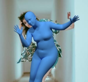
Figure A.4: Qualitative results of SHAPY predictions for female bodies.

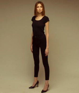
Figure A.5: Qualitative results of SHAPY predictions for female bodies. (Cont.)

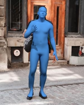
Figure A.6: Qualitative results of SHAPY predictions for male bodies.

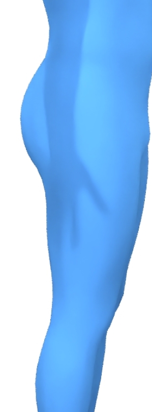
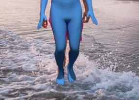
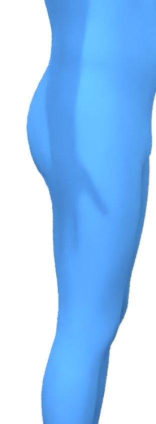
Figure A.7: Qualitative results of SHAPY predictions for male bodies (Cont.) .

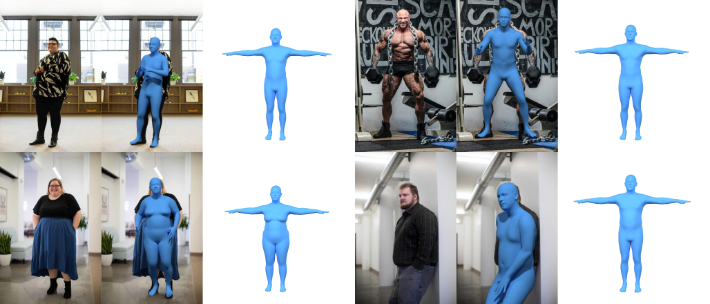
Figure A.8: Failure cases. In the first example (upper left) the weight is underestimated. Other failure cases of SHAPY are muscular bodies (upper right) and body shapes with high BMI (second row).