Federated Optimization Algorithms with Random Reshuffling and Gradient Compression

Abstract

Gradient compression is a popular technique for improving communication complexity of stochastic first-order methods in distributed training of machine learning models. However, the existing works consider only with-replacement sampling of stochastic gradients. In contrast, it is well-known in practice and recently confirmed in theory that stochastic methods based on without-replacement sampling, e.g., Random Reshuffling ( RR) method, perform better than ones that sample the gradients with-replacement. In this work, we close this gap in the literature and provide the first analysis of methods with gradient compression and without-replacement sampling. We first develop a naïve combination of random reshuffling with gradient compression ( Q-RR). Perhaps surprisingly, but the theoretical analysis of Q-RR does not show any benefits of using RR. Our extensive numerical experiments confirm this phenomenon. This happens due to the additional compression variance. To reveal the true advantages of RR in the distributed learning with compression, we propose a new method called DIANA-RR that reduces the compression variance and has provably better convergence rates than existing counterparts with with-replacement sampling of stochastic gradients. Next, to have a better fit to Federated Learning applications, we incorporate local computation, i.e., we propose and analyze the variants of Q-RR and DIANA-RR – Q-NASTYA and DIANA-NASTYA that use local gradient steps and different local and global stepsizes. Finally, we conducted several numerical experiments to illustrate our theoretical results.

1 Introduction

Federated learning (FL) (Konečný et al.,, 2016; McMahan et al.,, 2017) is a framework for distributed learning and optimization where multiple nodes connected over a network try to collaboratively carry out a learning task. Each node has its own dataset and cannot share its data with other nodes or with a central server, so algorithms for federated learning often have to rely on local computation and cannot access the entire dataset of training examples. Federated learning has applications in language modelling for mobile keyboards (Liu et al.,, 2021), healthcare (Antunes et al.,, 2022), wireless communications (Yang et al.,, 2022), and continues to find applications in many other areas (Kairouz et al.,, 2019).

Federated learning tasks are often solved through empirical-risk minimization (ERM), where the $m$-th devices contributes an empirical loss function $f_{m}(x)$ representing the average loss of model $x$ on its local dataset, and our goal is to then minimize the average loss over all the nodes:

$$\min_{x\in\mathbb{R}^{d}}\left[f(x)\overset{\rm def}{=}\frac{1}{M}\sum_{m=1}^{M}f_{m}(x)\right],$$ (1)

where the function $f$ represents the average loss. Every $f_{m}$ is an average of sample loss functions $f_{m}^{i}$ each representing the loss of model $x$ on the $i$-th datapoint on the $m$th clients’ dataset: that is for each $m\in\{1,2,\ldots,M\}$ we have

$$f_{m}(x)\overset{\rm def}{=}\frac{1}{n_{m}}\sum_{i=1}^{n_{m}}f_{m}^{i}(x).$$

For simplicity we shall assume that the datasets on all clients are of equal size: $n_{1}=n_{2}=\ldots=n_{M}$, though this assumption is only for convenience and our results easily extend to the case when clients have datasets of unequal sizes. Thus our optimization problem is

$$\min_{x\in\mathbb{R}^{d}}\left[f(x)=\frac{1}{nM}\sum_{m=1}^{M}\sum_{i=1}^{n}f_{m}^{i}(x)\right].$$ (2)

Because $d$ is often very large in practice, the dominant paradigm for solving (2) relies on first-order (gradient) information. Federated learning algorithms have access to two key primitives: (a) local computation, where for a given model $x\in\mathbb{R}^{d}$ we can compute stochastic gradients $\nabla f_{m}^{i}(x)$ locally on client $m$, and (b) communication, where the different clients can exchange their gradients or models with a central server.

1.1 Communication bottleneck: from one to multiple local steps

In practice, communication is more expensive than local computation (Kairouz et al.,, 2019), and as such one of the chief concerns of algorithms for federated learning is communication efficiency. Algorithms for federated learning have thus focused on achieving communication efficiency, with one common ingredient being the use of multiple local steps (Wang et al.,, 2021; Malinovskiy et al.,, 2020), where each node uses multiple gradients locally for several descent steps between communication steps. In general, algorithms using local steps fit the following pattern of generalized FedAvg (due to (Wang et al.,, 2021)); see Algorithm 1.

Algorithm 1 The generalized FedAvg framework for methods with local steps

1:$x_{0}$ – starting point, $\gamma>0$ – local stepsize, $\eta>0$ – global stepsize, $H$ - number of local steps

2:for communication rounds $t=0,1,\dots,T-1$ do

3:     for clients $m\in[M]$ in parallel do

4:         Receive $x_{t}$ from the server and set $x^{0}_{t,m}=x_{t}$

5:         for local steps $i=0,1,\dots,H$ do

6:              Set $x^{i+1}_{t,m}=\mathrm{ClientUpdate}(x_{t,m}^{i},\gamma,m,i)$          

7:         Send $x_{t,m}^{H}$ to the server, or alternatively send the update $\Delta_{t,m}=x_{t,m}^{H}-x_{t}$ to the server      

8:     Compute $x_{t+1}=\frac{1}{M}\sum_{m=1}^{M}x_{t,m}^{H}$ (or $x_{t+1}=x_{t}+\frac{1}{M}\sum_{m=1}^{M}\Delta_{t,m}$ if clients sent updates)

9:     Broadcast $x_{t+1}$ to the clients

10:$x_{T}$

When the client update method in Algorithm 1 is stochastic gradient descent, we get the FedAvg algorithm (also known as Local SGD). While FedAvg is popular in practice, recent theoretical progress has given tight analysis of the algorithm and shown that it can be definitively slower than its non-local counterparts (Khaled et al.,, 2020; Woodworth et al., 2020a, ; Glasgow et al.,, 2022). However, by using bias-reduction techniques one can use local steps and still maintain convergence rates at least as fast as non-local methods (Karimireddy et al.,, 2020), or in some cases even faster (Mishchenko et al.,, 2022). Thus local steps continue to be a useful algorithmic ingredient in both theory and practice for achieving communication efficiency.

1.2 Communication bottleneck: from full-dimensional to compressed communication

Another useful ingredient in distributed optimization is gradient compression, where each client sends a compressed or quantized version of their update $\Delta_{t,m}$ instead of the full update vector, potentially saving communication bandwidth by sending fewer bits over the network. There are many operators that can be used for compressing the update vectors: stochastic quantization (Alistarh et al.,, 2017), random sparsification (Wangni et al.,, 2018; Stich et al.,, 2018), and others (Tang et al.,, 2020). In this work we consider compression operators satisfying the following assumption:

Assumption 1.

A compression operator is an operator ${\cal Q}:\mathbb{R}^{d}\rightarrow\mathbb{R}^{d}$ such that for some $\omega>0$, the relations

$$\mathbb{E}\left[{\cal Q}(x)\right]=x\qquad\text{and}\qquad\mathbb{E}\left[\left\lVert{\cal Q}(x)-x\right\rVert^{2}\right]\leq\omega{\left\lVert x\right\rVert}^{2}$$

hold for $x\in\mathbb{R}^{d}$.

Unbiased compressors can reduce the number of bits clients communicate per round, but also increases the variance of the stochastic gradients used slowing down overall convergence, see e.g. (Khirirat et al.,, 2018, Theorem 5.2) and (Stich,, 2020, Theorem 1). By using control iterates, Mishchenko et al., 2019b developed DIANA—an algorithm that can reduce the variance due to gradient compression with unbiased compression operators, and thus ensure fast convergence. DIANA has been extended and analyzed in many settings (Horváth et al.,, 2019; Stich,, 2020; Safaryan et al.,, 2021) and forms an important tool in our arsenal for using gradient compression.

1.3 Communication bottleneck: from with replacement to without replacement sampling

The algorithmic framework of generalized FedAvg (Algorithm 1) requires specifying a client update method that is used locally on each client. The typical choice is stochastic gradient descent ( SGD), where at each time step we sample $j$ from $\{1,\ldots,n\}$ uniformly at random and then do a gradient descent step using the stochastic gradient $\nabla f_{m}^{j}(x_{t,m}^{i})$, resulting in the client update:

$$\mathrm{ClientUpdate}(x_{t,m}^{i},\gamma,m,i)=x_{t,m}^{i}-\gamma\nabla f_{m}^{j}(x_{t,m}^{i}).$$

This procedure thus uses with-replacement sampling in order to select the stochastic gradient used at each local step from the dataset on node $m$. In contrast, we can use without-replacement sampling to select the gradients: that is, at the beginning of each epoch we choose a permutation $\pi_{1},\pi_{2},\ldots,\pi_{n}$ of $\{1,2,\ldots,n\}$ and do the $i$-th update using the $\pi_{i}$-ith gradient:

$$\mathrm{ClientUpdate}(x_{t,m}^{i},\gamma,m,i)=x_{t,m}^{i}-\gamma\nabla f_{m}^{\pi_{i}}(x_{t,m}^{i}).$$

Without-replacement sampling SGD, also known as Random Reshuffling ( RR), typically achieves better asymptotic convergence rates compared to with-replacement SGD and can improve upon it in many settings as shown by recent theoretical progress (Mishchenko et al.,, 2020; Ahn et al.,, 2020; Rajput et al.,, 2020; Safran and Shamir,, 2021). While with-replacement SGD achieves an error proportional to $\mathcal{O}\left(\frac{1}{T}\right)$ after $T$ steps (Stich,, 2019), Random Reshuffling achieves an error of $\mathcal{O}\left(\frac{n}{T^{2}}\right)$ after $T$ steps, faster than SGD when the number of steps $T$ is large.

The success of RR in the single-machine setting has inspired several recent methods that use it as a local update method as part of distributed training: Mishchenko et al., (2021) developed a distributed variant of random reshuffling, FedRR. FedRR fits into the framework of Algorithm 1 and uses RR as a local client update method in lieu of SGD. They show that FedRR can improve upon the convergence of Local SGD when the number of local steps is fixed as the local dataset size, i.e. when $H=n$. Yun et al., (2021) study the same method under the name Local RR under a more restrictive assumption of bounded inter-machine gradient deviation and show that by varying $H$ to be smaller than $n$ better rates can be obtained in this setting than the rates of Mishchenko et al., (2021). Other work has explored more such combinations between RR and distributed training algorithms (Huang et al.,, 2021; Malinovsky et al.,, 2022; Horváth et al.,, 2022).

1.4 Three tricks for achieving communication efficiency

To summarize, we have at our disposal the following tricks and techniques for achieving communication efficiency in distributed training: (a) Local steps, (b) Gradient compression, and (c) Random Reshuffling. Each has found its use in federated learning and poses its own challenges, requiring special analysis or bias/variance-reduction techniques to achieve the best theoretical convergence rates and practical performance. Client heterogeneity causes local methods (with or without random reshuffling) to be biased, hence requiring bias-reduction techniques (Karimireddy et al.,, 2020; Murata and Suzuki,, 2021) or decoupling local and server stepsizes (Malinovsky et al.,, 2022). Gradient compression reduces the number of bits clients have to send per round, but causes an increase in variance, and we hence also need variance-reduction techniques to achieve better convergence rates under gradient compression (Mishchenko et al., 2019b, ; Stich and Karimireddy,, 2019). However, it is not clear apriori how these techniques should be combined to improve the convergence speed, and this is our starting point.

1.5 Contributions

In this paper, we aim to develop methods for federated optimization that combine gradient compression, random reshuffling, and/or local steps. While each of these techniques can aid in reducing the communication complexity of distributed optimization, their combination is under-explored. Thus our goal is to design methods that improve upon existing algorithms in convergence rates and in practice. We summarize our contributions as:

• The issue: naïve combination has no improvements. As a natural step towards our goal, we start with non-local methods and propose a new algorithm, Q-RR (Algorithm 2), that combines random reshuffling with gradient compression at every communication round. However, for Q-RR our theoretical results do not show any improvement upon QSGD when the compression level is reasonable. Moreover, we observe similar performance of Q-RR and QSGD in various numerical experiments. Therefore, we conclude that this phenomenon is not an artifact of our analysis but rather an issue of Q-RR: communication compression adds an additional noise that dominates the one coming from the stochastic gradients sampling.

• The remedy: reduction of compression variance. To remove the additional variance added by the compression and unleash the potential of Random Reshuffling in distributed learning with compression, we propose DIANA-RR (Algorithm 3), a combination of Q-RR and the DIANA algorithm. We derive the convergence rates of the new method and show that it improves upon the convergence rates of Q-RR, QSGD, and DIANA. We point out that to achieve such results we use $n$ shift-vectors per worker in DIANA-RR unlike DIANA that uses only $1$ shift-vector.

• Extensions to the local steps. Inspired by the NASTYA algorithm of Malinovsky et al., (2022), we propose a variant of NASTYA, Q-NASTYA (Algorithm 4), that naïvely mixes quantization, local steps with random reshuffling, and uses different local and server stepsizes. Although it improves in per-round communication cost over NASTYA but, similar to Q-RR, we show that Q-NASTYA suffers from added variance due to gradient quantization. To overcome this issue, we propose another algorithm, DIANA-NASTYA (Algorithm 5), that adds DIANA-style variance reduction to Q-NASTYA and removes the additional variance.

Finally, to illustrate our theoretical findings we conduct experiments on federated linear regression tasks.

1.6 Related work

Federated optimization has been the subject of intense study, with many open questions even in the setting when all clients have identical data (Woodworth et al., 2020b, ; Woodworth et al., 2020a, ; Woodworth et al.,, 2021). The FedAvg algorithm (also known as Local SGD) has also been a subject of intense study, with tight bounds obtained only very recently by Glasgow et al., (2022). It is now understood that using many local steps adds bias to distributed SGD, and hence several methods have been developed to mitigate it, e.g. (Karimireddy et al.,, 2020; Murata and Suzuki,, 2021), see the work of Gorbunov et al., (2021) for a unifying lens on many variants of Local SGD. Note that despite the bias, even vanilla FedAvg/ Local SGD still reduces the overall communication overhead in practice (Ortiz et al.,, 2021).

There are several methods that combine compression or quantization and local steps: both Basu et al., (2019) and Reisizadeh et al., (2020) combined Local SGD with quantization and sparsification, and Haddadpour et al., (2021) later improved their results using a gradient tracking method, achieving linear convergence under strong convexity. In parallel, Mitra et al., (2021) also developed a variance-reduced method, FedLin, that achieves linear convergence under strong convexity despite using local steps and compression. The paper most related to our work is (Malinovsky and Richtárik,, 2022) in which the authors combine iterate compression, random reshuffling, and local steps. We study gradient compression instead, which is a more common form of compression in both theory and practice (Kairouz et al.,, 2019). We compare our results against (Malinovsky and Richtárik,, 2022) and show we obtain better rates compared to their work.

2 Algorithms and Convergence Theory

We will primarily consider the setting of strongly-convex and smooth optimization. We assume that the average function $f$ is strongly convex:

Assumption 2.

Function $f:\mathbb{R}^{d}\rightarrow\mathbb{R}$ is $\mu$-strongly convex, i.e., for all $x,y\in\mathbb{R}^{d}$,

$$f(x)-f(y)-\langle\nabla f(y),x-y\rangle\geq\frac{\mu}{2}\|x-y\|^{2},$$ (3)

and functions $f^{i}_{1},f^{i}_{2},\dots,f^{i}_{M}:\mathbb{R}^{d}\rightarrow\mathbb{R}$ are convex for all $i=1,\dots,n$.

Examples of objectives satisfying Assumption 2 include $\ell_{2}$-regularized linear and logistic regression. Throughout the paper, we assume that $f$ has the unique minimizer $x_{*}\in\mathbb{R}^{d}$. We also use the assumption that each individual loss $f_{m}^{i}$ is smooth, i.e. has Lipschitz-continuous first-order derivatives:

Assumption 3.

Function $f^{i}_{m}:\mathbb{R}^{d}\rightarrow\mathbb{R}$ is $L_{i,m}$-smooth for every $i\in[n]$ and $m\in[M]$, i.e., for all $x,y\in\mathbb{R}^{d}$ and for all $m\in[M]$ and $i\in[n]$,

$$\|\nabla f^{i}_{m}(x)-\nabla f^{i}_{m}(y)\|\leq L_{i,m}\|x-y\|.$$ (4)

We denote the maximal smoothness constant as $L_{\max}\overset{\rm def}{=}\max_{i,m}L_{i,m}$.

For some methods, we shall additionally impose the assumption that each function is strongly convex:

Assumption 4.

Each function $f_{m}^{i}:\mathbb{R}^{d}\rightarrow\mathbb{R}$ is $\widetilde{\mu}$-strongly convex.

The Bregman divergence associated with a convex function $h$ is defined for all $x,y\in\mathbb{R}^{d}$ as

$$D_{h}(x,y)\overset{\rm def}{=}h(x)-h(y)-\left\langle\nabla h(y),x-y\right\rangle.$$

Note that the inequality (3) defining strong convexity can be compactly written as $D_{f}(x,y)\geq\frac{\mu}{2}\|x-y\|^{2}$.

2.1 Algorithm Q-RR

The first method we introduce is Q-RR (Algorithm 2). Q-RR is a straightforward combination of distributed random reshuffling and gradient quantization. This method can be seen as the stochastic without-replacement analogue of the distributed quantized gradient method of Khirirat et al., (2018).

Algorithm 2 Q-RR: Distributed Random Reshuffling with Quantization

1:$x_{0}$ – starting point, $\gamma>0$ – stepsize

2:for $t=0,1,\dots,T-1$ do

3:     Receive $x_{t}$ from the server and set $x^{0}_{t,m}=x_{t}$

4:     Sample random permutation of $[n]$: $\pi_{m}=(\pi^{0}_{m},\dots,\pi^{n-1}_{m})$

5:     for $i=0,1,\dots,n-1$ do

6:         for $m=1,\dots,M$ in parallel do

7:              Receive $x^{i}_{t}$ from the server, compute and send ${\cal Q}\left(\nabla f^{\pi^{i}_{m}}_{m}(x^{i}_{t})\right)$ back          

8:         Compute and send $x^{i+1}_{t}=x^{i}_{t}-\gamma\frac{1}{M}\sum^{M}_{m=1}{\cal Q}\left(\nabla f^{\pi^{i}_{m}}_{m}(x^{i}_{t})\right)$ to the workers      

9:     $x_{t+1}=x^{n}_{t}$

10:$x_{T}$

We shall the use the notion of shuffling radius defined by Mishchenko et al., (2021) for the analysis of distributed methods with random reshuffling:

Definition 1.

Define the iterate sequence $x^{i+1}_{\star}=x^{i}_{\star}-\frac{\gamma}{M}\sum^{M}_{m=1}\nabla f^{\pi^{i}_{m}}_{m}(x_{\star})$. Then the shuffling radius is the quantity

$$\sigma^{2}_{\text{rad}}\overset{\rm def}{=}\max_{i}\left\{\frac{1}{\gamma^{2}M}\sum^{M}_{m=1}\mathbb{E}D_{f^{\pi^{i}}_{m}}(x^{i}_{\star},x_{\star})\right\}.$$

We now state the main convergence theorem for Algorithm 2:

Theorem 1.

Let Assumptions 1, 3, 4 hold and let the stepsize satisfy $0<\gamma\leq\frac{1}{\left(1+2\frac{\omega}{M}\right)L_{\max}}.$ Then, for all $T\geq 0$ the iterates produced by Q-RR (Algorithm 2) satisfy

$$\mathbb{E}\|x_{T}-x_{\star}\|^{2} \leq \left(1-\gamma\widetilde{\mu}\right)^{nT}\|x_{0}-x_{\star}\|^{2}+\frac{2\gamma^{2}\sigma^{2}_{\text{rad}}}{\widetilde{\mu}}$$ (5)

$$\quad+\frac{2\gamma\omega}{\widetilde{\mu}M}(\zeta_{\star}^{2}+\sigma_{\star}^{2}),$$

where $\zeta^{2}_{\star}\overset{\rm def}{=}\frac{1}{M}\sum\limits_{m=1}^{M}\|\nabla f_{m}(x_{\star})\|^{2},$ and $\sigma_{\star}^{2}\overset{\rm def}{=}\frac{1}{Mn}\sum\limits_{m=1}^{M}\sum\limits_{i=1}^{n}\|\nabla f_{m}^{i}(x_{\star})-\nabla f_{m}(x_{\star})\|^{2}.$

All proofs are relegated to the appendix. By choosing the stepsize $\gamma$ properly, we can obtain the communication complexity (number of communication rounds) needed to find an $\varepsilon$-approximate solution as follows:

Corollary 1.

Under the same conditions as Theorem 1 and for Algorithm 2, there exists a stepsize $\gamma>0$ such that the number of communication rounds $nT$ to find a solution with accuracy $\varepsilon>0$ (i.e. $\mathbb{E}{\left\lVert x_{T}-x_{*}\right\rVert}^{2}\leq\epsilon$) is equal to

$$\widetilde{{\cal O}}\left(\left(1+\frac{\omega}{M}\right)\frac{L_{\max}}{\widetilde{\mu}}+\frac{\omega(\zeta^{2}_{\star}+\sigma_{\star}^{2})}{M\widetilde{\mu}^{2}\varepsilon}+\frac{\sigma_{\text{rad}}}{\sqrt{\widetilde{\mu}^{3}\varepsilon}}\right),$$ (6)

where $\widetilde{{\cal O}}(\cdot)$ hides constants and logarithmic factors.

The complexity of Quantized SGD ( QSGD) is (Gorbunov et al.,, 2020):

$$\widetilde{{\cal O}}\left(\left(1+\frac{\omega}{M}\right)\frac{L_{\max}}{\mu}+\frac{\left(\omega\zeta_{\star}^{2}+(1+\omega)\sigma_{\star}^{2}\right)}{M\mu^{2}\varepsilon}\right).$$

For simplicity, let us neglect the differences between $\mu$ and $\widetilde{\mu}$. First, when $\omega=0$ we recover the complexity of FedRR (Mishchenko et al.,, 2021) which is known to be better than the one of SGD as long as $\varepsilon$ is sufficently small as we have $\nicefrac{{n\mu\sigma_{\star}^{2}}}{{8}}\leq\sigma_{\text{rad}}^{2}\leq\nicefrac{{nL\sigma_{\star}^{2}}}{{4}}$ from (Mishchenko et al.,, 2021). Next, when $M=1$ and $\omega=0$ (single node, no compression) our results recovers the rate of RR (Mishchenko et al.,, 2020).

However, it is more interesting to compare Q-RR and QSGD when $M>1$ and $\omega>1$, which is typically the case. In these settings, Q-RR and QSGD have the same complexity since the ${\cal O}(\nicefrac{{1}}{{\varepsilon}})$ term dominates the ${\cal O}(\nicefrac{{1}}{{\sqrt{\varepsilon}}})$ one if $\varepsilon$ is sufficiently small. That is, the derived result for Q-RR has no advantages over the known one for QSGD unless $\omega$ is very small, which means that there is almost no compression at all. We also observe this phenomenon in the experiments.

The main reason for that is the variance appearing due to compression. Indeed, even if the current point is the solution of the problem ($x_{t}^{i}=x_{\ast}$), the update direction $-\gamma\frac{1}{M}\sum^{M}_{m=1}{\cal Q}\left(\nabla f^{\pi^{i}_{m}}_{m}(x^{i}_{t})\right)$ has the compression variance

$$\mathbb{E}_{{\cal Q}}\left[\left\|\frac{\gamma}{M}\sum^{M}_{m=1}\left({\cal Q}(\nabla f^{\pi^{i}_{m}}_{m}(x_{*}))-\nabla f^{\pi^{i}_{m}}_{m}(x_{*})\right)\right\|^{2}\right]\leq\frac{\gamma^{2}\omega}{M^{2}}\sum^{M}_{m=1}\|\nabla f^{\pi^{i}_{m}}_{m}(x_{*})\|^{2}.$$

This upper bound is tight and non-zero in general. Moreover, it is proportional to $\gamma^{2}$ that creates the term proportional to $\gamma$ in (5) like in the convergence results for QSGD/ SGD, while the RR-variance is proportional to $\gamma^{2}$ in the same bound. Therefore, during the later stages of the convergence Q-RR behaves similarly to QSGD when we decrease the stepsize.

2.2 Algorithm DIANA-RR

To reduce the additional variance caused by compression, we apply DIANA-style shift sequences (Mishchenko et al., 2019b, ; Horváth et al.,, 2019). Thus we obtain DIANA-RR (Algorithm 3). We notice that unlike DIANA, DIANA-RR has $n$ shift-vectors on each node.

Algorithm 3 DIANA-RR

1:$x_{0}$ – starting point, $\{h_{0,m}^{i}\}_{m,i=1,1}^{M,n}$ – initial shift-vectors, $\gamma>0$ – stepsize, $\alpha>0$ – stepsize for learning the shifts

2:for $t=0,1,\dots,T-1$ do

3:     Receive $x_{t}$ from the server and set $x^{0}_{t,m}=x_{t}$

4:     Sample random permutation of $[n]$: $\pi_{m}=(\pi^{0}_{m},\dots,\pi^{n-1}_{m})$

5:     for $i=0,1,\dots,n-1$ do

6:         for $m=1,2,\dots,M$ in parallel do

7:              Receive $x^{i}_{t}$ from the server, compute and send ${\cal Q}\left(\nabla f^{\pi^{i}_{m}}_{m}(x^{i}_{t})-h^{\pi^{i}_{m}}_{t,m}\right)$ back

8:              Set $\hat{g}^{\pi^{i}_{m}}_{t,m}=h^{\pi^{i}_{m}}_{t,m}+{\cal Q}\left(\nabla f^{\pi^{i}_{m}}_{m}(x^{i}_{t,m})-h^{\pi^{i}_{m}}_{t,m}\right)$

9:              Set $h^{\pi^{i}_{m}}_{t+1,m}=h^{\pi^{i}_{m}}_{t,m}+\alpha{\cal Q}\left(\nabla f^{\pi^{i}_{m}}_{m}(x^{i}_{t,m})-h^{\pi^{i}_{m}}_{t,m}\right)$          

10:         Compute $x^{i+1}_{t}=x^{i}_{t}-\gamma\frac{1}{M}\sum^{M}_{m=1}\hat{g}^{\pi^{i}_{m}}_{t,m}$ and send $x_{t}^{i+1}$ to the workers      

11:     $x_{t+1}=x^{n}_{t}$

12:$x_{T}$

Theorem 2.

Let Assumptions 1, 3, 4 hold and suppose that the stepsizes satisfy $0<\gamma\leq\min\left\{\frac{\alpha}{2n\widetilde{\mu}},\frac{1}{\left(1+\frac{6\omega}{M}\right)L_{\max}}\right\},$ and $\alpha\leq\frac{1}{1+\omega}.$ Define the following Lyapunov function for every $t\geq 0$

$$\Psi_{t+1} \overset{\rm def}{=} \|x_{t+1}-x_{\star}\|^{2}+\frac{4\omega\gamma^{2}}{\alpha M^{2}}\sum^{M}_{m=1}\sum^{n-1}_{j=0}(1-\gamma\mu)^{j}\|\Delta_{t+1,m}^{j}\|^{2},$$ (7)

where $\Delta_{t+1,m}^{j}=h^{\pi^{j}_{m}}_{t+1,m}-\nabla f^{\pi^{j}_{m}}_{m}(x_{\star})$ Then, for all $T\geq 0$ the iterates produced by DIANA-RR (Algorithm 3) satisfy

$$\mathbb{E}\left[\Psi_{T}\right]\leq\left(1-\gamma\widetilde{\mu}\right)^{nT}\Psi_{0}+\frac{2\gamma^{2}\sigma^{2}_{\text{rad}}}{\widetilde{\mu}}$$

Corollary 2.

Under the same conditions as Theorem 2 and for Algorithm 3, there exists stepsizes $\gamma,\alpha>0$ such that the number of communication rounds $nT$ to find a solution with accuracy $\varepsilon>0$ is

$$\widetilde{{\cal O}}\left(n(1+\omega)+\left(1+\frac{\omega}{M}\right)\frac{L_{\max}}{\widetilde{\mu}}+\frac{\sigma_{\text{rad}}}{\sqrt{\varepsilon\widetilde{\mu}^{3}}}\right).$$

Unlike Q-RR/ QSGD/ DIANA, DIANA-RR does not have a $\widetilde{\cal O}(\nicefrac{{1}}{{\varepsilon}})$-term, which makes it superior to Q-RR/ QSGD/ DIANA for small enough $\varepsilon$. However, the complexity of DIANA-RR has an additive $\widetilde{{\cal O}}(n(1+\omega))$ term arising due to learning the shifts $\{h_{t,m}^{i}\}_{m\in[M],i\in[n]}$. Nevertheless, this additional term is not the dominating one when $\varepsilon$ is small enough. Next, we elaborate a bit more on the comparison between DIANA and DIANA-R. That is, DIANA has $\widetilde{{\cal O}}\left(\left(1+\frac{\omega}{M}\right)\frac{L_{\max}}{\mu}+\frac{(1+\omega)\sigma_{\star}^{2}}{M\mu^{2}\varepsilon}\right)$ complexity (Gorbunov et al.,, 2020). Neglecting the differences between $\mu$ and $\widetilde{\mu}$, $L_{\max}$ and $L_{\max}$, we observe a similar relation between DIANA-RR and DIANA as between RR and SGD: instead of the term ${\cal O}(\nicefrac{{(1+\omega)\sigma_{\star}^{2}}}{{(M\mu^{2}\varepsilon)}})$ appearing in the complexity of DIANA, DIANA-RR has ${\cal O}(\nicefrac{{\sigma_{\text{rad}}}}{{\sqrt{\varepsilon\widetilde{\mu}^{3}}}})$ term much better depending on $\varepsilon$. To the best of our knowledge, our result is the only known one establishing the theoretical superiority of RR to regular SGD in the context of distributed learning with gradient compression. Moreover, when $\omega=0$ (no compression) we recover the rate of FedRR and when additionally $M=1$ (single worker) we recover the rate of RR.

2.3 Algorithm Q-NASTYA

By adding local steps to Q-RR, we can do enable each client to do more local work and only communicate once per epoch rather than at each iteration of every epoch. We follow the framework of the NASTYA algorithm (Malinovsky et al.,, 2022) and extend it by allowing for quantization, resulting in Q-NASTYA (Algorithm 4).

Algorithm 4 Q-NASTYA

1:$x_{0}$ – starting point, $\gamma>0$ – local stepsize, $\eta>0$ – global stepsize

2:for $t=0,1,\dots,T-1$ do

3:     for $m\in[M]$ in parallel do

4:         Receive $x_{t}$ from the server and set $x^{0}_{t,m}=x_{t}$

5:         Sample random permutation of $[n]$: $\pi_{m}=(\pi^{0}_{m},\dots,\pi^{n-1}_{m})$

6:         for $i=0,1,\dots,n-1$ do

7:              Set $x^{i+1}_{t,m}=x^{i}_{t,m}-\gamma\nabla f^{\pi^{i}_{m}}_{m}(x^{i}_{t,m})$          

8:         Compute $g_{t,m}=\frac{1}{\gamma n}\left(x_{t}-x^{n}_{t,m}\right)$ and send ${\cal Q}_{t}(g_{t,m})$ to the server      

9:     Compute $g_{t}=\frac{1}{M}\sum_{m=1}^{M}\mathcal{Q}_{t}(g_{t,m})$

10:     Compute $x_{t+1}=x_{t}-\eta g_{t}$ and send $x_{t+1}$ to the workers

11:$x_{T}$

Theorem 3.

Let Assumptions 1, 2, 3 hold. Let the stepsizes $\gamma$, $\eta$ satisfy $0<\eta\leq\frac{1}{16L_{\max}\left(1+\frac{\omega}{M}\right)},$ $0<\gamma\leq\frac{1}{5nL_{\max}}.$ Then, for all $T\geq 0$ the iterates produced by Q-NASTYA (Algorithm 4) satisfy

$$\mathbb{E}\left[\|x_{T}-x_{\star}\|^{2}\right] \leq \left(1-\frac{\eta\mu}{2}\right)^{T}\|x_{0}-x_{\star}\|^{2}+\frac{9}{2}\frac{\gamma^{2}nL_{\max}}{\mu}\left((n+1)\zeta^{2}_{\star}+\sigma_{\star}^{2}\right)+8\frac{\eta\omega}{\mu M}\zeta^{2}_{\star}.$$

Corollary 3.

Under the same conditions as Theorem 3 and for Algorithm 4, there exist stepsizes $\gamma=\nicefrac{{\eta}}{{n}}$ and $\eta>0$ such that the number of communication rounds $T$ to find a solution with accuracy $\varepsilon>0$ is

$$\widetilde{{\cal O}}\left(\frac{L_{\max}}{\mu}\left(1+\frac{\omega}{M}\right)+\frac{\omega}{M}\frac{\zeta^{2}_{\star}}{\varepsilon\mu^{3}}+\sqrt{\frac{L_{\max}}{\varepsilon\mu^{3}}}\sqrt{\zeta^{2}_{\star}+\frac{\sigma_{\star}^{2}}{n}}\right).$$

If $\gamma\rightarrow 0$, one can choose $\eta>0$ such that the above complexity bound improves to

$$\widetilde{{\cal O}}\left(\frac{L_{\max}}{\mu}\left(1+\frac{\omega}{M}\right)+\frac{\omega}{M}\frac{\zeta^{2}_{\star}}{\varepsilon\mu^{3}}\right).$$

We emphasize several differences with the known theoretical results. First, the FedCOM method of Haddadpour et al., (2021) was analyzed in the homogeneous setting only, i.e., $f_{m}(x)=f(x)$ for all $m\in[M]$, which is an unrealistic assumption for FL applications. In contrast, our result holds in the fully heterogeneous case. Next, the analysis of FedPAQ of  Reisizadeh et al., (2020) uses a bounded variance assumption, which is also known to be restrictive. Nevertheless, let us compare to their result. Reisizadeh et al., (2020) derive the following complexity for their method:

$$\widetilde{{\cal O}}\left(\frac{L_{\max}}{\mu}\left(1+\frac{\omega}{M}\right)+\frac{\omega}{M}\frac{\sigma^{2}}{\mu^{2}\varepsilon}+\frac{\sigma^{2}}{M\mu^{2}\varepsilon}\right).$$

This result is inferior to the one we show for Q-NASTYA: when $\omega$ is small, the main term in the complexity bound of FedPAQ is $\widetilde{{\cal O}}\left(\nicefrac{{1}}{{\varepsilon}}\right)$, while for Q-NASTYA the dominating term is of the order $\widetilde{{\cal O}}\left(\nicefrac{{1}}{{\sqrt{\varepsilon}}}\right)$ (when $\omega$ and $\varepsilon$ are sufficiently small). We also highlight that FedCRR (Malinovsky and Richtárik,, 2022) does not converge if $\omega>\nicefrac{{M^{2}\gamma\mu\varepsilon}}{{(2\left\|x_{*,m}^{n}\right\|^{2})}}$, while Q-NASTYA does for any $\omega\geq 0$. Finally, when $\omega=0$ (no compression) we recover NASTYA as a special case, and using $\gamma=\nicefrac{{\eta}}{{n}}$, we recover the rate of FedRR (Mishchenko et al.,, 2021).

2.4 Algorithm DIANA-NASTYA

As in the case of Q-RR, the complexity bound for Q-NASTYA includes a $\widetilde{\cal O}(\nicefrac{{\omega}}{{\varepsilon}})$ term, appearing due to quantization noise. To reduce it, we apply DIANA-style correction sequences, which leads to a new method for which we coin the name DIANA-NASTYA (Algorithm 5).

Algorithm 5 DIANA-NASTYA

1:$x_{0}$ – starting point, $\{h_{0,m}\}_{m=1}^{M}$ – initial shift-vectors, $\gamma>0$ – local stepsize, $\eta>0$ – global stepsize, $\alpha>0$ – stepsize for learning the shifts

2:for $t=0,1,\dots,T-1$ do

3:     for $m=1,\dots,M$ in parallel do

4:         Receive $x_{t}$ from the server and set $x^{0}_{t,m}=x_{t}$

5:         Sample random permutation of $[n]$: $\pi_{m}=(\pi^{0}_{m},\dots,\pi^{n-1}_{m})$

6:         for $i=0,1,\dots,n-1$ do

7:              Set $x^{i+1}_{t,m}=x^{i}_{t,m}-\gamma\nabla f^{\pi^{i}_{m}}_{m}(x^{i}_{t,m})$          

8:         Compute $g_{t,m}=\frac{1}{\gamma n}\left(x_{t}-x^{n}_{t,m}\right)$ and send ${\cal Q}_{t}\left(g_{t,m}-h_{t,m}\right)$ to the server

9:         Set $h_{t+1,m}=h_{t,m}+\alpha{\cal Q}_{t}\left(g_{t,m}-h_{t,m}\right)$

10:         Set $\hat{g}_{t,m}=h_{t,m}+{\cal Q}_{t}\left(g_{t,m}-h_{t,m}\right)$      

11:     $h_{t+1}=\frac{1}{M}\sum^{M}_{m=1}h_{t+1,m}=h_{t}+\frac{\alpha}{M}\sum^{M}_{m=1}{\cal Q}_{t}\left(g_{t,m}-h_{t,m}\right)$

12:     $\hat{g}_{t}=\frac{1}{M}\sum^{M}_{m=1}\hat{g}_{t,m}=h_{t}+\frac{1}{M}\sum^{M}_{m=1}{\cal Q}_{t}\left(g_{t,m}-h_{t,m}\right)$

13:     $x_{t+1}=x_{t}-\eta\hat{g}_{t}$

14:$x_{T}$

Theorem 4.

Let Assumptions 1, 2, 3 hold. Suppose the stepsizes $\gamma$, $\eta,\alpha$ satisfy $0<\gamma\leq\frac{1}{16L_{\max}n}$, $0<\eta\leq\min\left\{\frac{\alpha}{2\mu},\frac{1}{16L_{\max}\left(1+\frac{9\omega}{M}\right)}\right\},$ and $\alpha\leq\frac{1}{1+\omega}.$ Define the following Lyapunov function:

$$\Psi_{t+1}\overset{\rm def}{=}\|x_{t+1}-x_{\star}\|^{2}+\frac{8\omega\eta^{2}}{\alpha M^{2}}\sum^{M}_{m=1}\|h_{t+1,m}-h^{\star}_{m}\|^{2}.$$ (8)

Then, for all $T\geq 0$ the iterates produced by DIANA-NASTYA (Algorithm 5) satisfy

$$\mathbb{E}\left[\Psi_{T}\right]\leq\left(1-\frac{\eta\mu}{2}\right)^{T}\Psi_{0}+\frac{9}{2}\frac{\gamma^{2}nL}{\mu}\left((n+1)\zeta^{2}_{\star}+\sigma_{\star}^{2}\right).$$ (9)

Corollary 4.

Under the same conditions as Theorem 4 and for Algorithm 5, there exist stepsizes $\gamma=\nicefrac{{\eta}}{{n}}$, $\eta>0$, $\alpha>0$ such that the number of communication rounds $T$ to find a solution with accuracy $\varepsilon>0$ is

$$\widetilde{{\cal O}}\left(\omega+\frac{L_{\max}}{\mu}\left(1+\frac{\omega}{M}\right)+\sqrt{\frac{L_{\max}}{\varepsilon\mu^{3}}}\sqrt{\zeta^{2}_{\star}+\frac{\sigma_{\star}^{2}}{n}}\right).$$

If $\gamma\rightarrow 0$, one can choose $\eta>0$ such that the above complexity bound improves to

$$\widetilde{{\cal O}}\left(\omega+\frac{L_{\max}}{\mu}\left(1+\frac{\omega}{M}\right)\right).$$

In contrast to Q-NASTYA, DIANA-NASTYA does not suffer from the $\widetilde{{\cal O}}(\nicefrac{{1}}{{\varepsilon}})$ term in the complexity bound. This shows the superiority of DIANA-NASTYA to Q-NASTYA. Next, FedCRR-VR (Malinovsky and Richtárik,, 2022) has the rate

$$\widetilde{\mathcal{O}}\left(\frac{(\omega+1)\left(1-\frac{1}{\kappa}\right)^{n}}{\left(1-\left(1-\frac{1}{\kappa}\right)^{n}\right)^{2}}+\frac{\sqrt{\kappa}\left(\zeta_{\star}+\sigma_{\star}\right)}{\mu\sqrt{\varepsilon}}\right),$$

which depends on $\widetilde{{\cal O}}\left(\nicefrac{{1}}{{\sqrt{\varepsilon}}}\right)$. However, the first term is close to $\widetilde{{\cal O}}\left((\omega+1)\kappa^{2}\right)$ for a large condition number. FedCRR-VR-2 utilizes variance reduction technique from Malinovsky et al., (2021) and it allows to get rid of permutation variance. This method has

$$\widetilde{{\cal O}}\left(\frac{(\omega+1)\left(1-\frac{1}{\kappa\sqrt{\kappa n}}\right)^{\frac{n}{2}}}{\left(1-\left(1-\frac{1}{\kappa\sqrt{\kappa n}}\right)^{\frac{n}{2}}\right)^{2}}+\frac{\sqrt{\kappa}\zeta_{\star}}{\mu\sqrt{\varepsilon}}\right)$$

complexity, but it requires additional assumption on number of functions $n$ and thus not directly comparable with our result. Note that if we have no compression $(\omega=0)$, DIANA-NASTYA recovers rate of NASTYA.

3 Experiments

We tested our methods on solving a logistic regression problem and in training neural networks.

3.1 Logistic Regression

To confirm our theoretical results we conducted several numerical experiments on binary classification problem with L2 regularized logistic regression of the form

$$\min_{x\in\mathbb{R}^{d}}\left[f(x)\overset{\rm def}{=}\frac{1}{M}\sum_{m=1}^{M}\frac{1}{n_{m}}\sum_{i=1}^{n_{m}}f_{m,i}\right]\text{, }$$ (10)

where $f_{m,i}\overset{\rm def}{=}\log\left(1+\exp({-y_{mi}a_{mi}^{\top}x})\right)+\lambda\|x\|^{2}_{2}$ $(a_{mi},y_{mi})\in\mathbb{R}^{d}\times\in\{-1,1\},i=1,\dots,n_{m}$ are the training data samples stored on machines $m=1,\dots,M$, and $\lambda>0$ is a regularization parameter. In all experiments, for each method, we used the largest stepsize allowed by its theory multiplied by some individually tuned constant multiplier. For better parallelism, each worker $m$ uses mini-batches of size $\approx 0.1n_{m}$. In all algorithms, as a compression operator ${\cal Q}$, we use Rand-$k$ (Beznosikov et al.,, 2020) with fixed compression ratio $\nicefrac{{k}}{{d}}\approx 0.02$, where $d$ is the number of features in the dataset. We provide more details on experimental setups, hardware and datasets in Appendix A.

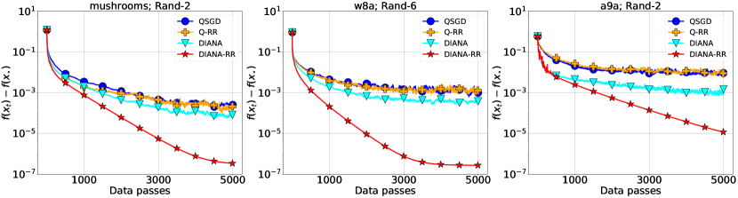
(a) Non-local methods

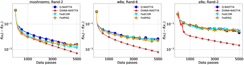
(b) Local methods

Figure 1: The comparison of the four proposed methods ( Q-NASTYA, DIANA-NASTYA, Q-RR, DIANA-RR) and existing baselines ( FedCOM, FedPAQ) with tuned stepsizes and Rand-$k$ compressor.

Experiment 1: Comparison of the proposed non-local methods with existing baselines.

In our first experiment (see Figure 1(a)), we compare Q-RR and DIANA-RR with corresponding classical baselines ( QSGD (Alistarh et al.,, 2017), DIANA (Mishchenko et al., 2019b, )) that use a with-replacement mini-batch SGD estimator. Figure 1(a) illustrates that Q-RR experiences similar behavior as QSGD both losing in speed to DIANA method in all considered datasets. However, DIANA-RR shows the best rate among all considered non-local methods, efficiently reducing the variance, and achieving the lowest functional sub-optimality tolerance. The results observed in numerical experiments are in perfect correspondence with the derived theory.

Experiment 2: Comparison of the proposed local methods with existing baselines.

The second experiment shows that DIANA-based method can significantly outperform in practice when one applies it to local methods as well. In particular, whereas Q-NASTYA shows comparative behavior as existing methods FedCOM (Haddadpour et al.,, 2021), FedPAQ (Reisizadeh et al.,, 2020) in all considered datasets, DIANA-NASTYA noticeably outperforms other methods.

3.2 Training ResNet-18 on CIFAR10

Since random reshuffling is a very popular technique in training neural networks, it is natural to test the proposed methods on such problems. Therefore, in the second set of experiments, we consider training ResNet-18 (He et al.,, 2016) model on the CIFAR10 dataset Krizhevsky and Hinton, (2009). To conduct these experiments we use FL_PyTorch simulator (Burlachenko et al.,, 2021). Further technical details are deferred to Appendix A.

Experiment 3: Comparison of the proposed non-local methods in training ResNet-18 on CIFAR10.

The main goal of this experiment is to verify the phenomenon observed in Experiment 1 on the training of a deep neural network. That is, we tested Q-RR, QSGD, DIANA, and DIANA-RR in the distributed training of ResNet-18 on CIFAR10, see Figure 2. As in the logistic regression experiments, we observe that (i) Q-RR and QSGD behave similarly and (ii) DIANA-RR outperforms DIANA.

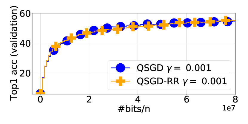
(a) Q-RR vs QSGD

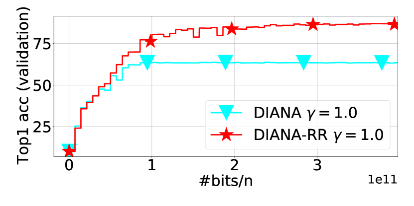
(b) DIANA-RR vs DIANA

Figure 2: The comparison of Q-RR, QSGD, DIANA, and DIANA-RR on the task of training ResNet-18 on CIFAR-10 with $n=10$ workers. Top-1 accuracy on test set is reported. Stepsizes were tuned and workers used Rand-$k$ compressor with $\nicefrac{{k}}{{d}}\approx 0.05$. Further details and additional experiments are provided in Appendix A.

Appendix A Experiments: Missing Details and Extra Results

In this section, we provide missing details on the experimental setting from Section 3. The codes are provided in the following Github repository: https://github.com/IgorSokoloff/rr_with_compression_experiments_source_code.

A.1 Logistic Regression

Hardware and Software.

All algorithms were written in Python 3.8. We used three different CPU cluster node types:

1. AMD EPYC 7702 64-Core;

2. Intel(R) Xeon(R) Gold 6148 CPU @ 2.40GHz;

3. Intel(R) Xeon(R) Gold 6248 CPU @ 2.50GHz.

Datasets.

The datasets were taken from open LibSVM library Chang and Lin, (2011), sorted in ascending order of labels, and equally split among 20 machines $\backslash$clients$\backslash$workers. The remaining part of size $N-20\cdot\left\lfloor{\nicefrac{{N}}{{20}}}\right\rfloor$ was assigned to the last worker, where $N=\sum_{m=1}^{M}n_{m}$ is the total size of the dataset. A summary of the splitting and the data samples distribution between clients can be found in Tables 1, 2, 3, 4.

Table 1: Summary of the datasets and splitting of the data samples among clients.

Dataset	$M$	$N$ (dataset size)	$d$ (# of features)	$n_{m}$ (# of datasamples per client)
mushrooms	$20$	$8120$	$112$	$406$
w8a	$20$	$49749$	$300$	$2487$
a9a	$20$	$32560$	$123$	$1628$

Table 2: Partition of the mushrooms dataset among clients.

Client’s №	# of datasamples of class "-1"	# of datasamples of class "+1"
$1$ – $9$	$406$	$0$
$10$	$262$	$144$
$11$ – $19$	$0$	$406$
$20$	$0$	$410$

Table 3: Partition of the w8a dataset among clients.

Client’s №	# of datasamples of class "-1"	# of datasamples of class "+1"
$1$ – $19$	$2487$	$0$
$20$	$1017$	$1479$

Table 4: Partition of the a9a dataset among clients.

Client’s №	# of datasamples of class "-1"	# of datasamples of class "+1"
$1$ – $14$	$1628$	$0$
$15$	$1328$	$300$
$16$ – $19$	$0$	$1628$
$20$	$0$	$1629$

Hyperparameters.

Regularization parameter $\lambda$ was chosen individually for each dataset to guarantee the condition number $\nicefrac{{L}}{{\mu}}$ to be approximately $10^{4}$, where $L$ and $\mu$ are the smoothness and strong-convexity constants of function $f$. For the chosen logistic regression problem of the form (10), smoothness and strong convexity constants $L$, $L_{m}$, $L_{i,m}$, $\mu$, $\widetilde{\mu}$ of functions $f$, $f_{m}$ and $f_{m}^{i}$ were computed explicitly as

$$L = \lambda_{max}\left(\frac{1}{M}\sum_{m=1}^{M}\frac{1}{4n_{m}}{\bf A}_{m}^{\top}{\bf A}_{m}+2\lambda{\bf I}\right)$$

$$L_{m} = \lambda_{max}\left(\frac{1}{4n_{m}}{\bf A}_{m}^{\top}{\bf A}_{m}+2\lambda{\bf I}\right)$$

$$L_{i,m} = \lambda_{\max}\left(\frac{1}{4}a_{mi}a_{mi}^{\top}+2\lambda{\bf I}\right)$$

$$\mu = 2\lambda$$

$$\widetilde{\mu} = 2\lambda,$$

where ${\bf A}_{m}$ is the dataset associated with client $m$, and $a_{mi}$ is the $i$-th row of data matrix ${\bf A}_{m}$. In general, the fact that $f$ is $L$-smooth with

$$L\leq\frac{1}{M}\sum_{m=1}^{M}\frac{1}{n_{m}}\sum_{i=1}^{n_{m}}L_{i,m}$$

follows from the $L_{i,m}$-smoothness of $f_{m}^{i}$ (see Assumption 3).

In all algorithms, as a compression operator ${\cal Q}$, we use Rand-$k$ as a canonical example of unbiased compressor with relatively bounded variance, and fix the compression parameter $k=\lfloor 0.02d\rfloor$, where $d$ is the number of features in the dataset.

In addition, in all algorithms, for all clients $m=1,\dots,M$, we set the batch size for the SGD estimator to be $b_{m}=\lfloor 0.1n_{m}\rfloor$, where $n_{m}$ is the size of the local dataset.

The summary of the values $L$, $L_{m}$, $L_{i,m}$ $L_{\max}$, $\mu$, $b_{m}$ and $k$ for each dataset can be found in Table 5.

Table 5: Summary of the hyperparameters.

Dataset	$L$	$L_{\max}$	$\mu$	$\lambda$	$k$	$b_{m}$ (batchsize)
mushrooms	$2.59$	$5.25$	$2.58\cdot 10^{-4}$	$1.29\cdot 10^{-4}$	$2$	$40$
w8a	$0.66$	$28.5$	$6.6\cdot 10^{-5}$	$3.3\cdot 10^{-5}$	$6$	$248$
a9a	$1.57$	$3.5$	$1.57\cdot 10^{-4}$	$7.85\cdot 10^{-5}$	$2$	$162$

In all experiments, we follow constant stepsize strategy within the whole iteration procedure. For each method, we set the largest possible stepsize predicted by its theory multiplied by some individually tuned constant multiplier. For a more detailed explanation of the tuning routine, see Sections A.1.1 and A.1.2.

SGD implementation.

We considered two approaches to minibatching: random reshuffling and with-replacement sampling. In the first, all clients $m=1,\dots,M$ independently permute their local datasets and pass through them within the next subsequent $\lfloor\frac{n_{m}}{b_{m}}\rfloor$ steps. In our implementations of Q-RR, Q-NASTYA and DIANA-NASTYA, all clients permuted their datasets in the beginning of every new epoch, whereas for the DIANA-RR method they do so only once in the beginning of the iteration procedure. Second approach of minibatching is called with-replacement sampling, and it requires every client to draw $b_{m}$ data samples from the local dataset uniformly at random. We used this strategy in the baseline algorithms ( QSGD, DIANA, FedCOM and FedPAQ) we compared our proposed methods to.

Experimental setup.

To compare the performance of methods within the whole optimization process, we track the functional suboptimality metric $f(x_{t})-f(x_{\star})$ that was recomputed after each epoch. For each dataset, the value $f(x_{\star})$ was computed once at the preprocessing stage with $10^{-16}$ tolerance via conjugate gradient method. We terminate our algorithms after performing $5000$ epochs.

A.1.1 Experiment 1: Comparison of the Proposed Non-Local Methods with Existing Baselines (Extra Details)

For each of the considered non-local methods, we take the stepsize as the largest one predicted by the theory premultiplied by the individually tuned constant factor from the set $\left\{0.000975,0.00195,0.0039,0.0078,0.0156,0.0312,0.0625,0.125,0.25,0.5,1,2,4,8,16,32,64,\right.$
$\left.128,256,512,1024,2048,4096\right\}.$

Therefore, for each local method on every dataset, we performed $20$ launches to find the stepsize multiplier showing the best convergence behavior (the fastest reaching the lowest possible level of functional suboptimality $f(x_{t})-f(x_{\star})$).

Theoretical stepsizes for methods Q-RR and DIANA-RR are provided by the Theorems 1 and 2, whereas stepsizes for QSGD and DIANA were taken from the paper Gorbunov et al., (2020).

A.1.2 Experiment 2: Comparison of the Proposed Local Methods with Existing Baselines (Extra Details)

In this set of experiments, we tuned stepsizes similarly to the non-local methods. However, for algorithms Q-NASTYA, DIANA-NASTYA, and FedCOM we needed to independently adjust the client and server stepsizes, leading to a more extensive tunning routine.

As before, for each local method on every dataset, tuned client and server stepsizes are defined by the theoretical one and adjusted constant multiplier. Theoretical stepsizes for methods Q-NASTYA and DIANA-NASTYA are given by the Theorems 3 and 4, whereas FedCOM and FedPAQ stepsizes were taken from the papers by Haddadpour et al., (2021) and Reisizadeh et al., (2020) respectively. We now list all the considered multipliers of client and server stepsizes for every method (i.e. $\gamma$ and $\eta$ respectively):

• Q-NASTYA:

  • Multipliers for $\gamma:$ $\{$0.000975, 0.00195, 0.0039, 0.0078, 0.0156, 0.0312, 0.0625, 0.125, 0.25, 0.5, 1, 2, 4, 8, 16, 32, 64,128$\}$;

  • Multipliers for $\eta:$ $\{$0.0039, 0.0078, 0.0156, 0.0312, 0.0625, 0.125, 0.25, 0.5, 1, 2, 4, 8, 16, 32, 64, 128$\}$.

• DIANA-NASTYA:

  • Multipliers for $\gamma$ and $\eta:$ $\{$0.000975, 0.00195, 0.0039, 0.0078, 0.0156, 0.0312, 0.0625, 0.125, 0.25, 0.5, 1, 2, 4, 8, 16, 32, 64,128$\}$;

• FedCOM:

  • Multipliers for $\gamma:$ $\{$0.0312, 0.0625, 0.125, 0.25, 0.5, 1, 2, 4, 8, 16, 32, 64, 128, 256, 512,1024, 2048, 4096, 8192, 16384, 32768 $\}$;

  • Multipliers for $\eta:$ $\{$0.000975, 0.00195, 0.0039, 0.0078, 0.0156, 0.0312, 0.0625, 0.125, 0.25, 0.5, 1, 2, 4, 8, 16, 32, 64, 128$\}$.

• FedPAQ:

  • Multipliers for $\gamma:$ $\{$0.00195, 0.0039, 0.0078, 0.0156, 0.0312, 0.0625, 0.125, 0.25, 0.5, 1, 2, 4, 8, 16, 32, 64, 128, 256, 512, 1024, 2048, 4096, 8192, 16384, 32768, 65536, 131072, 262144, 524288, 1048576 $\}$.

For example, to find the best pair $(\gamma,\eta)$ for FedCOM method on each dataset, we performed $378$ launches. A similar subroutine was executed for all algorithms on all datasets independently.

A.2 Training Deep Neural Network model: ResNet-18 on CIFAR-10

To illustrate the behavior of the proposed methods in training Deep Neural Networks (DNN), we consider the ResNet-18 (He et al.,, 2016) model. This model is used for image classification, feature extraction for image segmentation, object detection, image embedding, and image captioning. We train all layers of ResNet-18 model meaning that the dimension of the optimization problem equals $d=11,173,962$. During the training, the ResNet-18 model normalizes layer inputs via exploiting $20$ Batch Normalization  (Ioffe and Szegedy,, 2015) layers that are applied directly before nonlinearity in the computation graph of this model. Batch normalization (BN) layers add $9600$ trainable parameters to the model. Besides trainable parameters, a BN layer has its internal state that is used for computing the running mean and variance of inputs due to its own specific regime of working. We use He initialization (He et al.,, 2015).

A.2.1 Computing Environment

We performed numerical experiments on a server-grade machine running Ubuntu 18.04 and Linux Kernel v5.4.0, equipped with 16-cores (2 sockets by 16 cores per socket) 3.3 GHz Intel Xeon, and four NVIDIA A100 GPU with 40GB of GPU memory. The distributed environment is simulated in Python 3.9 via using the software suite FL_PyTorch  (Burlachenko et al.,, 2021) that serves for carrying complex Federate Learning experiments. FL_PyTorch allowed us to simulate the distributed environment in the local machine. Besides storing trainable parameters per client, this simulator stores all not trainable parameters including BN statistics per client.

A.2.2 Loss Function

Training of ResNet-18 can be formalized as problem (1) with the following choice of $f_{m}^{i}$

$$f_{m}(x)=\frac{1}{|n_{m}|}\sum_{j=1}^{|n_{m}|}CE(b^{(j)},g(a^{(j)},x)),$$ (11)

where $CE(p,q)\overset{\rm def}{=}-\sum_{k=1}^{\mathrm{\#classes}}p_{i}\cdot\log(q_{i})$ with agreement $0\cdot\log(0)=0$ is a standard cross-entropy loss, function $g:\mathbb{R}^{28\times 28}\times\mathbb{R}^{d}\to[0,1]^{\mathrm{\#classes}}$ is a neural network taking image $a^{(j)}$ and vector of parameters $x$ as an input and returning a vector in probability simplex, and $n_{m}$ is the size of the dataset on worker $m$.

A.2.3 Dataset and Metric

In our experiments, we used CIFAR10 dataset Krizhevsky and Hinton, (2009). The dataset consists of input variables $a_{i}\in\mathbb{R}^{28\times 28\times 3}$, and response variables $b_{i}\in\{0,1\}^{10}$ and is used for training 10-way classification. The sizes of training and validation set are $5\times 10^{4}$ and $10^{4}$ respectively. The training set is partitioned heterogeneously across $10$ clients. To measure the performance, we evaluate the loss function value $f(x)$, norm of the gradient $\|\nabla f(x)\|_{2}$ and the Top-1 accuracy of the obtained model as a function of passed epochs and the normalized number of bits sent from clients to the server.

A.2.4 Tuning Process

In this set of experiments, we tested QSGD (Alistarh et al.,, 2017), Q-RR (Algorithm 2), DIANA (Mishchenko et al., 2019a, ) and DIANA-RR (Algorithm 3) algorithms. For all algorithms, we tuned the strategy $\in\{A,B,C\}$ of decaying stepsize model via selecting the best in terms of the norm of the full gradient on the train set in the final iterate produced after $20000$ rounds. The stepsize policies are described below.

1. Stepsizes decaying as inverse square root of the number epochs

   $$\gamma_{e}=\begin{cases}\gamma_{init}\cdot\dfrac{1}{\sqrt{e-s+1}},&\text{if }e\geq s,\\ \gamma_{init},&\text{if }e<s,\end{cases}$$

   where $\gamma_{e}$ denotes the stepsize used during epoch $e+1$, $s$ is a fixed shift.

2. Stepsizes decaying as inverse of number epochs

   $$\gamma=\begin{cases}\gamma_{init}\cdot\dfrac{1}{{e-s+1}},&\text{if }e\geq s,\\ \gamma_{init},&\text{if }e<s.\end{cases}$$

3. Fixed stepsize

   $$\gamma=\gamma_{init}.$$

We say that the algorithm passed $e$ epochs if the total number of computed gradient oracles lies between $e\sum_{m=1}^{M}n_{m}$ and $(e+1)\sum_{m=1}^{M}n_{m}$. For each algorithm the used stepsize $\gamma_{init}$ and shift parameter $s$ were tuned via selecting from the following sets:

$$\gamma_{init}\in\gamma_{set}\overset{\rm def}{=}\{4.0,3.75,3.00,2.5,2.00,1.25,1.0,0.75,0.5,0.25,$$

$$0.2,0.1,0.06,0.03,0.01,0.003,0.001,0.0006\}.$$

$$s\in s_{set}\overset{\rm def}{=}\{50,100,200,500,1000\}.$$

In all tested methods, clients independently apply Rand-$k$ compression with carnality $k=\lfloor 0.05d\rfloor$. Computation for all gradient oracles is carried out in single precision float (fp32) arithmetic.

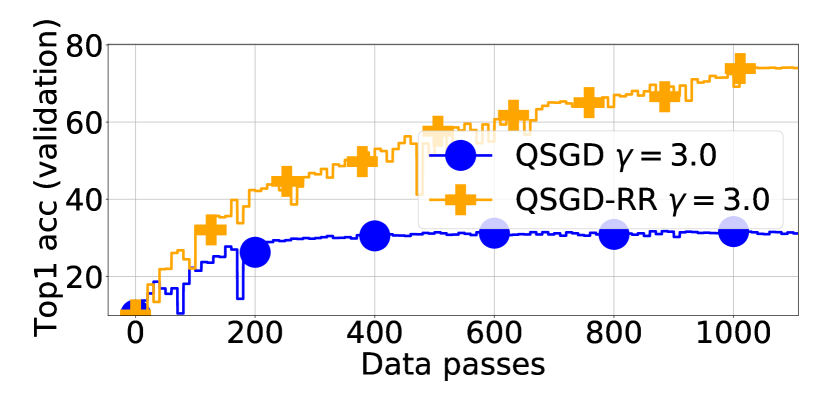
(a)

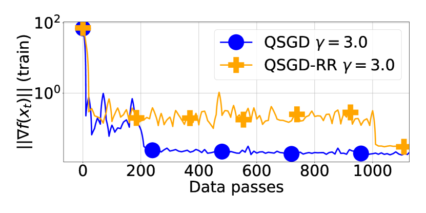
(b)

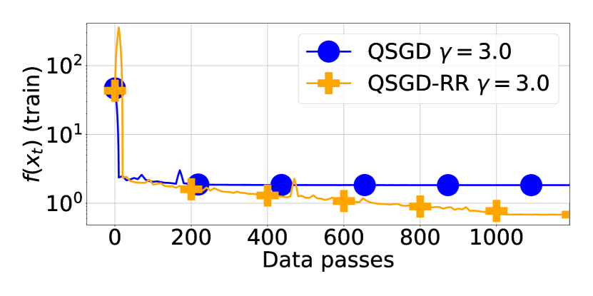
(c)

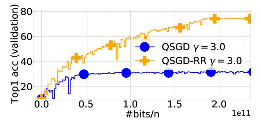
(d)

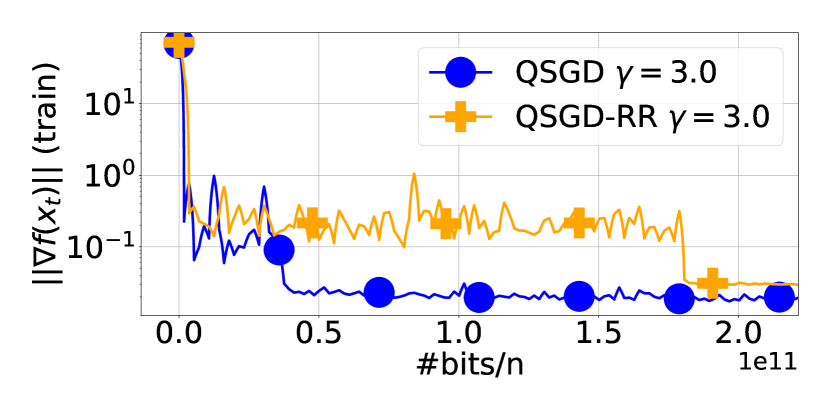
(e)

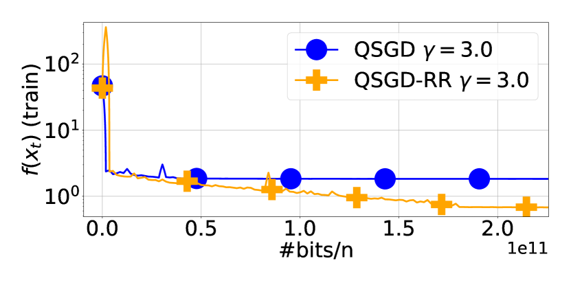
(f)

Figure 3: Comparison of QSGD and Q-RR in the training of ResNet-18 on CIFAR-10, with $n=10$ workers. Here (a) and (d) show Top-1 accuracy on test set, (b) and (e) – norm of full gradient on the train set, (c) and (f) – loss function value on the train set. Stepsizes and decay shift has been tuned from $s_{set}$ and $\gamma_{set}$ based on minimum achievable value of loss function on the train set.

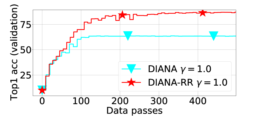
(a)

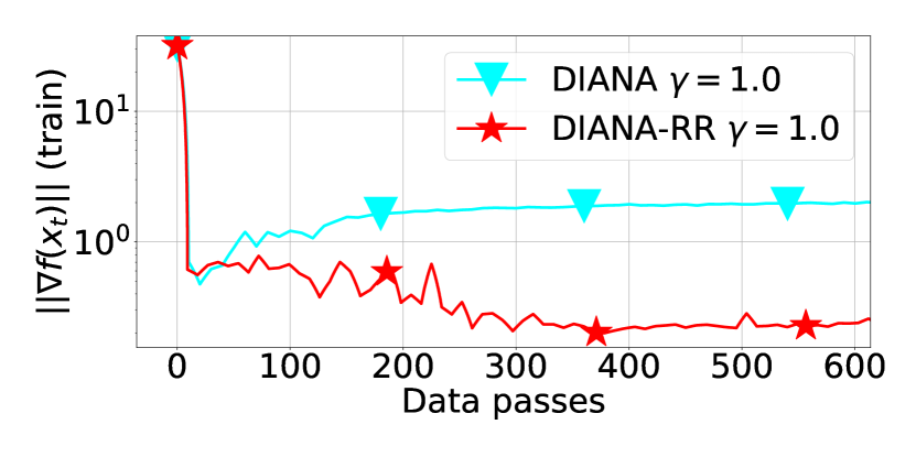
(b)

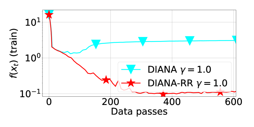
(c)

(d)

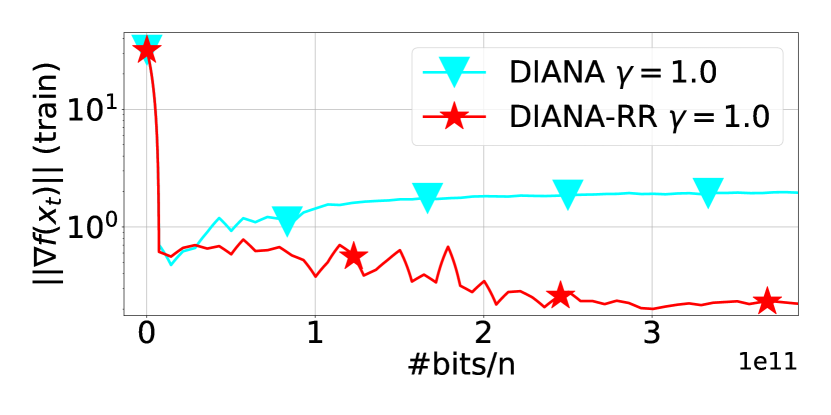
(e)

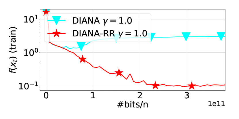
(f)

Figure 4: Comparison of DIANA and DIANA-RR in the training of ResNet-18 on CIFAR-10, with $n=10$ workers. Here (a) and (d) show Top-1 accuracy on test set, (b) and (e) – norm of full gradient on the train set, (c) and (f) – loss function value on the train set. Stepsizes and decay shift has been tuned from $s_{set}$ and $\gamma_{set}$ based on minimum achievable value of loss function on the train set. For both algorithms stepsize is fixed. For both algorithms stepsize is decaying according to srategy $B$.

A.2.5 Optimization-Based Fine-Tuning for Pretrained ResNet-18.

In this setting, we trained ResNet-18 image classification in a distributed way across $n=10$ clients. In this experiment, we have trained only the last linear layer.

Next, we have turned off batch normalization. Turning off batch normalization implies that the computation graph of NN $g(a,x)$ with weights of NN denoted as $x$ is a deterministic function and does not include any internal state.

The loss function is a standard cross-entropy loss augmented with extra $\ell_{2}$-regularization $\alpha\nicefrac{{\|x\|^{2}}}{{2}}$ with $\alpha=0.0001$. Initially used weights of NN are pretrained parameters after training the model on ImageNet.

The dataset distribution across clients has been set in a heterogeneous manner via presorting dataset $D$ by label class and after this, it was split across $10$ clients.

The comparison of stepsizes policies used in QSGD and Q-RR is presented in Figure 6. The behavior of the algorithms with best tuned step sizes is presented in Figure 5. These results demonstrate that in this setting there is no real benefit of using Q-RR in comparison to QSGD.

A.2.6 Experiments

The comparison of QSGD and Q-RR is presented in Figure 3. In particular, Figures 3(b) and 3(e) show that in terms of the convergence to stationary points both algorithms exhibit similar behavior. However, Q-RR has better generalization and in fact, converges to the better loss function value. This experiment demonstrates that Q-RR with manually tuned stepsize can be better compared to QSGD in terms of the final quality of obtained Deep Learning model. For QSGD the tuned meta parameters are: $\gamma_{init}=3.0$,$s=200$, $\text{strategy}=B$. For QSGD-RR tuned meta parameters are: $\gamma_{init}=3.0$, $s=1000$, $\text{strategy}=B$.

The results of comparison of DIANA and DIANA-RR are presented in Figure 4. For DIANA the tuned meta parameters are: $\gamma_{init}=1.0$,$s=0$, $\text{strategy}=C$ and for DIANA-RR tuned meta parameters are: $\gamma_{init}=1.0$, $s=0$, $\text{strategy}=C$. These results show that DIANA-RR outperforms DIANA in terms of the all reported metrics.

(a)

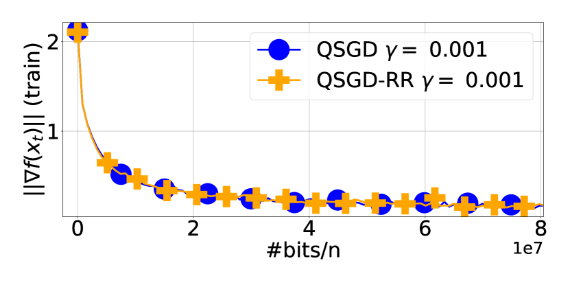
(b)

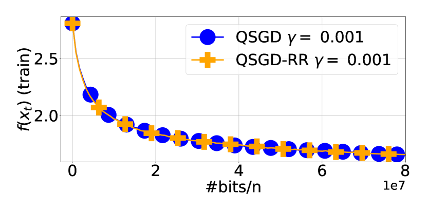
(c)

Figure 5: Comparison of QSGD and Q-RR in the training of the last linear layer of ResNet-18 on CIFAR-10, with $n=10$ workers. Here (a) shows Top-1 accuracy on test set, (b) – norm of full gradient on the train set, (c) – loss function value on the train set. Stepsizes and decay shift has been tuned from $s_{set}$ and $\gamma_{set}$ based on minimum achievable value of loss function on the train set. Both algorithms used fixed stepsize during training.

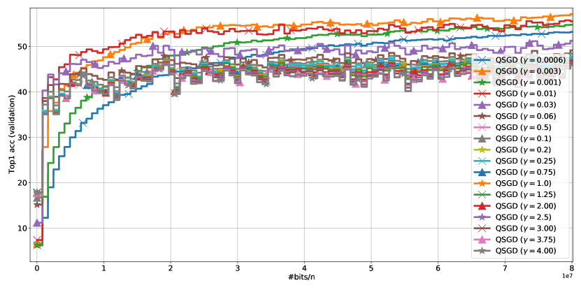
(a)

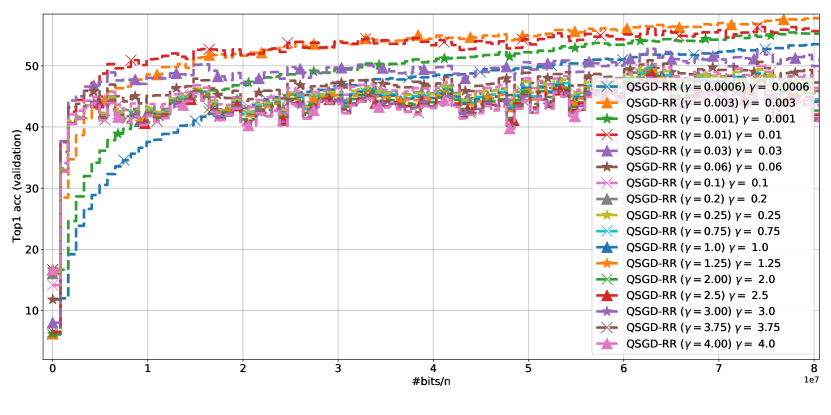
(b)

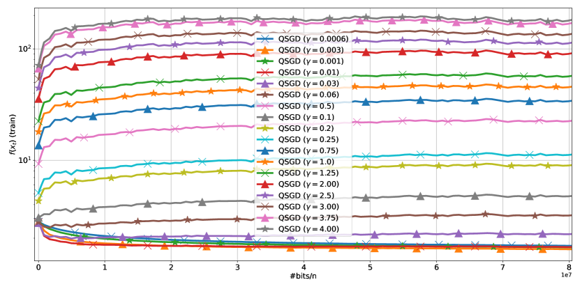
(c)

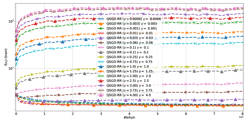
(d)

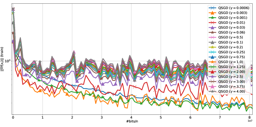
(e)

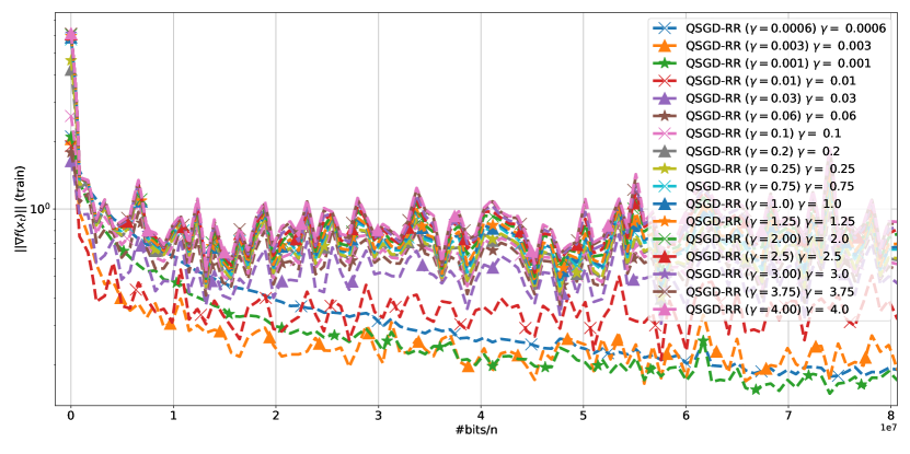
(f)

Figure 6: Comparison of QSGD and Q-RR in the training of the last linear layer of ResNet-18 on CIFAR-10, with $n=10$ workers. Here (a) and (b) show Top-1 accuracy on test set, (c) and (d) – loss function value on the train set, (e) and (f) – norm of full gradient on the train set. Stepsizes and decay shift has been tuned from $s_{set}$ and $\gamma_{set}$ based on minimum achievable value of loss function on the train set. During training stepsize was fixed. Batch Normalization was turned off.

Appendix B Missing Proofs For Q-RR

In the main part of the paper, we intoduce Assumptions 3 and 4 for the analysis of Q-RR and DIANA-RR. These assumptions can be refined as follows.

Assumption 5.

Function $f^{\pi^{i}}=\frac{1}{M}\sum^{M}_{i=1}f^{\pi_{m}^{i}}_{m}:\mathbb{R}^{d}\rightarrow\mathbb{R}$ is $\widetilde{L}$-smooth for all sets of permutations $\pi=(\pi_{1},\ldots,\pi_{m})$ from $[n]$ and all $i\in[n]$, i.e.,

$$\max_{i\in[n],\pi}\|\nabla f^{\pi^{i}}(x)-\nabla f^{\pi^{i}}(y)\|\leq\widetilde{L}\|x-y\|\quad\forall x,y\in\mathbb{R}^{d}.$$

Assumption 6.

Function $f^{\pi^{i}}=\frac{1}{M}\sum^{M}_{i=1}f^{\pi_{m}^{i}}_{m}:\mathbb{R}^{d}\rightarrow\mathbb{R}$ is $\widetilde{\mu}$-strongly convex for all sets of permutations $\pi=(\pi_{1},\ldots,\pi_{m})$ from $[n]$ and all $i\in[n]$, i.e.,

$$\min_{i\in[n],\pi}\left\{f^{\pi^{i}}(x)-f^{\pi^{i}}(y)-\langle\nabla f^{i,\pi}(y),x-y\rangle\right\}\geq\frac{\widetilde{\mu}}{2}\|x-y\|^{2}\quad\forall x,y\in\mathbb{R}^{d}.$$

Moreover, functions $f^{i}_{1},f^{i}_{2},\dots,f^{i}_{M}:\mathbb{R}^{d}\rightarrow\mathbb{R}$ are convex for all $i=1,\dots,n$.

We notice that Assumptions 3 and 4 imply Assumptions 5 and 6. Moreover, $\widetilde{L}\leq L_{\max}$. In the proofs of the results for Q-RR and DIANA-RR, we use Assumptions 5 in addition to Assumption 3 and we use Assumption 6 instead of Assumption 4.

B.1 Proof of Theorem 1

For convenience, we restate the theorem below.

Theorem 5 (Theorem 1).

Let Assumptions 1, 3, 5, 6 hold and $0<\gamma\leq\frac{1}{\widetilde{L}+2\frac{\omega}{M}L_{\max}}$. Then, for all $T\geq 0$ the iterates produced by Q-RR (Algorithm 2) satisfy

$$\mathbb{E}\|x_{T}-x_{\star}\|^{2}\leq\left(1-\gamma\widetilde{\mu}\right)^{nT}\|x_{0}-x_{\star}\|^{2}+\frac{2\gamma^{2}\sigma^{2}_{\text{rad}}}{\widetilde{\mu}}+\frac{2\gamma\omega}{\widetilde{\mu}M}\left(\zeta^{2}_{\star}+\sigma^{2}_{\star}\right),$$

where $\zeta^{2}_{\star}\overset{\rm def}{=}\frac{1}{M}\sum\limits_{m=1}^{M}\|\nabla f_{m}(x_{\star})\|^{2},$ and $\sigma_{\star}^{2}\overset{\rm def}{=}\frac{1}{Mn}\sum\limits_{m=1}^{M}\sum\limits_{i=1}^{n}\|\nabla f_{m}^{i}(x_{\star})-\nabla f_{m}(x_{\star})\|^{2}.$

Proof.

Using $x^{i+1}_{\star}=x^{i}_{\star}-\frac{\gamma}{M}\sum^{M}_{m=1}\nabla f^{\pi^{i}_{m}}_{m}(x_{\star})$ and line 7 of Algorithm 2, we get

$$\|x^{i+1}_{t}-x^{i+1}_{\star}\|^{2} = \left\|x^{i}_{t}-x^{i}_{\star}-\gamma\frac{1}{M}\sum^{M}_{m=1}\left({\cal Q}\left(\nabla f^{\pi^{i}_{m}}_{m}(x^{i}_{t})\right)-\nabla f^{\pi^{i}_{m}}_{m}(x_{\star})\right)\right\|^{2}$$

$$= \left\|x^{i}_{t}-x^{i}_{\star}\right\|^{2}-2\gamma\left\langle\frac{1}{M}\sum^{M}_{m=1}\left({\cal Q}\left(\nabla f^{\pi^{i}_{m}}_{m}(x^{i}_{t})\right)-\nabla f^{\pi^{i}_{m}}_{m}(x_{\star})\right),x^{i}_{t}-x^{i}_{\star}\right\rangle$$

$$+\gamma^{2}\left\|\frac{1}{M}\sum^{M}_{m=1}\left({\cal Q}\left(\nabla f^{\pi^{i}_{m}}_{m}(x^{i}_{t})\right)-\nabla f^{\pi^{i}_{m}}_{m}(x_{\star})\right)\right\|^{2}.$$

Taking the expectation w.r.t. ${\cal Q}$, we obtain

$$\mathbb{E}_{{\cal Q}}\left[\|x^{i+1}_{t}-x^{i+1}_{\star}\|^{2}\right] = \left\|x^{i}_{t}-x^{i}_{\star}\right\|^{2}-2\gamma\left\langle\frac{1}{M}\sum^{M}_{m=1}\left(\nabla f^{\pi^{i}_{m}}_{m}(x^{i}_{t})-\nabla f^{\pi^{i}_{m}}_{m}(x_{\star})\right),x^{i}_{t}-x^{i}_{\star}\right\rangle$$

$$+\gamma^{2}\mathbb{E}_{{\cal Q}}\left[\left\|\frac{1}{M}\sum^{M}_{m=1}\left({\cal Q}\left(\nabla f^{\pi^{i}_{m}}_{m}(x^{i}_{t})\right)-\nabla f^{\pi^{i}_{m}}_{m}(x_{\star})\right)\right\|^{2}\right].$$

In view of Assumption 1 and $\mathbb{E}_{\xi}\|\xi-c\|^{2}=\mathbb{E}_{\xi}\|\xi-\mathbb{E}_{\xi}\xi\|^{2}+\|\mathbb{E}_{\xi}\xi-c\|^{2}$, we have

$$\mathbb{E}_{{\cal Q}}\left[\|x^{i+1}_{t}-x^{i+1}_{\star}\|^{2}\right] = \left\|x^{i}_{t}-x^{i}_{\star}\right\|^{2}-\frac{2\gamma}{M}\sum^{M}_{m=1}\left\langle\nabla f^{\pi^{i}_{m}}_{m}(x^{i}_{t})-\nabla f^{\pi^{i}_{m}}_{m}(x_{\star}),x^{i}_{t}-x^{i}_{\star}\right\rangle$$

$$+\gamma^{2}\mathbb{E}_{{\cal Q}}\left[\left\|\frac{1}{M}\sum^{M}_{m=1}\left({\cal Q}\left(\nabla f^{\pi^{i}_{m}}_{m}(x^{i}_{t})\right)-\nabla f^{\pi^{i}_{m}}_{m}(x^{i}_{t})\right)\right\|^{2}\right]$$

$$+\gamma^{2}\left\|\frac{1}{M}\sum^{M}_{m=1}\left(\nabla f^{\pi^{i}_{m}}_{m}(x^{i}_{t})-\nabla f^{\pi^{i}_{m}}_{m}(x_{\star})\right)\right\|^{2}$$

$$\leq \left\|x^{i}_{t}-x^{i}_{\star}\right\|^{2}-\frac{2\gamma}{M}\sum^{M}_{m=1}\left\langle\nabla f^{\pi^{i}_{m}}_{m}(x^{i}_{t})-\nabla f^{\pi^{i}_{m}}_{m}(x_{\star}),x^{i}_{t}-x^{i}_{\star}\right\rangle$$

$$+\gamma^{2}\left\|\frac{1}{M}\sum^{M}_{m=1}\left(\nabla f^{\pi^{i}_{m}}_{m}(x^{i}_{t})-\nabla f^{\pi^{i}_{m}}_{m}(x_{\star})\right)\right\|^{2}+\frac{\gamma^{2}\omega}{M^{2}}\sum^{M}_{m=1}\left\|\nabla f^{\pi^{i}_{m}}_{m}(x^{i}_{t})\right\|^{2},$$

where in the last step we apply independence of ${\cal Q}\left(\nabla f^{\pi^{i}_{m}}_{m}(x^{i}_{t})\right)$ for $m\in[M]$. Next, we use three-point identity and obtain

$$\mathbb{E}_{{\cal Q}}\left[\|x^{i+1}_{t}-x^{i+1}_{\star}\|^{2}\right] \leq \left\|x^{i}_{t}-x^{i}_{\star}\right\|^{2}-\frac{2\gamma}{M}\sum^{M}_{m=1}\left(D_{f^{\pi^{i}_{m}}_{m}}(x^{i}_{\star},x^{i}_{t})+D_{f^{\pi^{i}_{m}}_{m}}(x^{i}_{t},x_{\star})-D_{f^{\pi^{i}_{m}}_{m}}(x^{i}_{\star},x_{\star})\right)$$

$$+\gamma^{2}\left\|\frac{1}{M}\sum^{M}_{m=1}\left(\nabla f^{\pi^{i}_{m}}_{m}(x^{i}_{t})-\nabla f^{\pi^{i}_{m}}_{m}(x_{\star})\right)\right\|^{2}+\frac{\gamma^{2}\omega}{M^{2}}\sum^{M}_{m=1}\left\|\nabla f^{\pi^{i}_{m}}_{m}(x^{i}_{t})\right\|^{2}.$$

Applying $\widetilde{L}$-smoothness and convexity of $\frac{1}{M}\sum_{m=1}^{m}f_{m}^{\pi_{m}^{i}}$, $\widetilde{\mu}$-strong convexity of $\frac{1}{M}\sum_{m=1}^{m}f_{m}^{\pi_{m}^{i}}$, and $L_{\max}$-smoothness and convexity of $f_{m}^{i}$, we get

$$\mathbb{E}_{{\cal Q}}\left[\|x^{i+1}_{t}-x^{i+1}_{\star}\|^{2}\right] \leq \left(1-\gamma\widetilde{\mu}\right)\left\|x^{i}_{t}-x^{i}_{\star}\right\|^{2}-2\gamma\left(1-\widetilde{L}\gamma\right)\frac{1}{M}\sum^{M}_{m=1}D_{f^{\pi^{i}_{m}}_{m}}(x^{i}_{t},x_{\star})$$

$$+2\gamma\frac{1}{M}\sum^{M}_{m=1}D_{f^{\pi^{i}_{m}}_{m}}(x^{i}_{\star},x_{\star})+\frac{\gamma^{2}\omega}{M^{2}}\sum^{M}_{m=1}\left\|\nabla f^{\pi^{i}_{m}}_{m}(x^{i}_{t})\right\|^{2}$$

$$\leq \left(1-\gamma\widetilde{\mu}\right)\left\|x^{i}_{t}-x^{i}_{\star}\right\|^{2}-2\gamma\left(1-\widetilde{L}\gamma\right)\frac{1}{M}\sum^{M}_{m=1}D_{f^{\pi^{i}_{m}}_{m}}(x^{i}_{t},x_{\star})$$

$$+2\gamma\frac{1}{M}\sum^{M}_{m=1}D_{f^{\pi^{i}_{m}}_{m}}(x^{i}_{\star},x_{\star})+\frac{2\gamma^{2}\omega}{M^{2}}\sum^{M}_{m=1}\left\|\nabla f^{\pi^{i}_{m}}_{m}(x_{\star})\right\|^{2}$$

$$+\frac{2\gamma^{2}\omega}{M^{2}}\sum^{M}_{m=1}\left\|\nabla f^{\pi^{i}_{m}}_{m}(x^{i}_{t})-\nabla f^{\pi^{i}_{m}}_{m}(x_{\star})\right\|^{2}$$

$$\leq \left(1-\gamma\widetilde{\mu}\right)\left\|x^{i}_{t}-x^{i}_{\star}\right\|^{2}+\frac{2\gamma^{2}\omega}{M^{2}}\sum^{M}_{m=1}\left\|\nabla f^{\pi^{i}_{m}}_{m}(x_{\star})\right\|^{2}+\frac{2\gamma}{M}\sum^{M}_{m=1}D_{f^{\pi^{i}_{m}}_{m}}(x^{i}_{\star},x_{\star})$$

$$-2\gamma\left(1-\gamma\left(\widetilde{L}+\frac{2\omega L_{\max}}{M}\right)\right)\frac{1}{M}\sum^{M}_{m=1}D_{f^{\pi^{i}_{m}}_{m}}(x^{i}_{t},x_{\star}).$$

Taking the full expectation and using a definition of shuffle radius, $0<\gamma\leq\frac{1}{\left(\widetilde{L}+2\frac{\omega}{M}L_{\max}\right)}$, and $D_{f^{\pi^{i}_{m}}_{m}}(x^{i}_{t},x_{\star})\geq 0$, we obtain

$$\mathbb{E}\left[\|x^{i+1}_{t}-x^{i+1}_{\star}\|^{2}\right] \leq \left(1-\gamma\widetilde{\mu}\right)\mathbb{E}\left[\left\|x^{i}_{t}-x^{i}_{\star}\right\|^{2}\right]+2\gamma^{3}\sigma^{2}_{\text{rad}}+\frac{2\gamma^{2}\omega}{M^{2}}\sum^{M}_{m=1}\mathbb{E}\left[\left\|\nabla f^{\pi^{i}_{m}}_{m}(x_{\star})\right\|^{2}\right]$$

$$= \left(1-\gamma\widetilde{\mu}\right)\mathbb{E}\left[\left\|x^{i}_{t}-x^{i}_{\star}\right\|^{2}\right]+2\gamma^{3}\sigma^{2}_{\text{rad}}+\frac{2\gamma^{2}\omega}{M^{2}n}\sum^{M}_{m=1}\sum^{n}_{j=1}\left\|\nabla f^{j}_{m}(x_{\star})\right\|^{2}$$

$$\leq \left(1-\gamma\widetilde{\mu}\right)\mathbb{E}\left[\left\|x^{i}_{t}-x^{i}_{\star}\right\|^{2}\right]+2\gamma^{3}\sigma^{2}_{\text{rad}}+\frac{2\gamma^{2}\omega}{M}\left(\zeta^{2}_{\star}+\sigma^{2}_{\star}\right).$$

Unrolling the recurrence in $i$, we derive

$$\mathbb{E}\left[\|x_{t+1}-x_{\star}\|^{2}\right] \leq \left(1-\gamma\widetilde{\mu}\right)^{n}\mathbb{E}\left[\left\|x_{t}-x_{\star}\right\|^{2}\right]+2\gamma^{3}\sigma^{2}_{\text{rad}}\sum^{n-1}_{j=0}(1-\gamma\widetilde{\mu})^{j}$$

$$+\frac{2\gamma^{2}\omega}{M}\left(\zeta^{2}_{\star}+\sigma^{2}_{\star}\right)\sum^{n-1}_{j=0}(1-\gamma\widetilde{\mu})^{j}.$$

Unrolling the recurrence in $t$, we derive

$$\mathbb{E}\left[\|x_{T}-x_{\star}\|^{2}\right] \leq \left(1-\gamma\widetilde{\mu}\right)^{nT}\left\|x_{0}-x_{\star}\right\|^{2}+2\gamma^{3}\sigma^{2}_{\text{rad}}\sum^{T-1}_{t=0}(1-\gamma\widetilde{\mu})^{nt}\sum^{n-1}_{j=0}(1-\gamma\widetilde{\mu})^{j}$$

$$+\frac{2\gamma^{2}\omega}{M}\left(\zeta^{2}_{\star}+\sigma^{2}_{\star}\right)\sum^{nT-1}_{j=0}(1-\gamma\widetilde{\mu})^{nt}\sum^{n-1}_{j=0}(1-\gamma\widetilde{\mu})^{j}.$$

Since $\sum^{nT-1}_{j=0}(1-\gamma\widetilde{\mu})^{j}\leq\frac{1}{\gamma\widetilde{\mu}}$, we get the result. ∎

Corollary 5.

Let the assumptions of Theorem 5 hold and

$$\gamma=\min\left\{\frac{1}{\widetilde{L}+2\frac{\omega}{M}L_{\max}},\sqrt{\frac{\varepsilon\widetilde{\mu}}{6\sigma^{2}_{\text{rad}}}},\frac{\varepsilon\widetilde{\mu}M}{6\omega\left(\zeta^{2}_{\star}+\sigma^{2}_{\star}\right)}\right\}.$$ (12)

Then, Q-RR (Algorithm 2) finds a solution with accuracy $\varepsilon>0$ after the following number of communication rounds:

$$\widetilde{{\cal O}}\left(\frac{\widetilde{L}}{\widetilde{\mu}}+\frac{\omega}{M}\frac{L_{\max}}{\widetilde{\mu}}+\frac{\omega}{M}\frac{\zeta^{2}_{\star}+\sigma^{2}_{\star}}{\varepsilon\widetilde{\mu}^{2}}+\frac{\sigma_{\text{rad}}}{\sqrt{\varepsilon\widetilde{\mu}^{3}}}\right).$$

Proof.

Theorem 5 implies

$$\mathbb{E}\|x_{T}-x_{\star}\|^{2}\leq\left(1-\gamma\widetilde{\mu}\right)^{nT}\|x_{0}-x_{\star}\|^{2}+\frac{2\gamma^{2}\sigma^{2}_{\text{rad}}}{\widetilde{\mu}}+\frac{2\gamma\omega}{\widetilde{\mu}M}\left(\zeta^{2}_{\star}+\sigma^{2}_{\star}\right).$$ (13)

To estimate the number of communication rounds required to find a solution with accuracy $\varepsilon>0$, we need to upper-bound each term from the right-hand side by $\nicefrac{{\varepsilon}}{{3}}$. Thus, we get additional conditions on $\gamma$:

$$\frac{2\gamma^{2}\sigma^{2}_{\text{rad}}}{\widetilde{\mu}}<\frac{\varepsilon}{3},\qquad\frac{2\gamma\omega}{\widetilde{\mu}M}\left(\zeta^{2}_{\star}+\sigma^{2}_{\star}\right)<\frac{\varepsilon}{3}$$

and also the upper bound on the number of communication rounds $nT$

$$nT=\widetilde{{\cal O}}\left(\frac{1}{\gamma\widetilde{\mu}}\right).$$

Substituting (12), we get a final result. ∎

B.2 Non-Strongly Convex Summands

In this section, we provide the analysis of Q-RR without using Assumptions 4, 6. Before we move one to the proofs, we would like to emphasize that

$$x^{i+1}_{t}=x^{i}_{t}-\gamma\frac{1}{M}\sum^{M}_{m=1}{\cal Q}\left(\nabla f^{\pi^{i}_{m}}_{m}(x^{i}_{t})\right).$$

Then we have

$$x_{t+1}=x_{t}-\gamma\sum^{n-1}_{i=0}\frac{1}{M}\sum^{M}_{m=1}{\cal Q}\left(\nabla f^{\pi^{i}_{m}}_{m}(x^{i}_{t})\right)=x_{t}-\tau\frac{1}{Mn}\sum^{n-1}_{i=0}\sum^{M}_{m=1}{\cal Q}\left(\nabla f^{\pi^{i}_{m}}_{m}(x^{i}_{t})\right),$$

where $\tau=\gamma n$. For convenience, we denote

$$g_{t}\overset{\rm def}{=}\frac{1}{Mn}\sum^{n-1}_{i=0}\sum^{M}_{m=1}{\cal Q}\left(\nabla f^{\pi^{i}_{m}}_{m}(x^{i}_{t})\right),$$

which allows us to write the update rule as $x_{t+1}=x_{t}-\tau g_{t}$.

Lemma 1 (Lemma 1 from  (Malinovsky et al.,, 2022)).

For any $k\in[n]$, let $\xi_{\pi_{1}},\dots,\xi_{\pi_{k}}$ be sampled uniformly without replacement from a set of vectors $\{\xi_{1},\dots,\xi_{n}\}$ and $\bar{\xi}_{\pi}$ be their average. Then

$$\mathbb{E}\bar{\xi}_{\pi}=\bar{\xi},\qquad\mathbb{E}\left[\|\bar{\xi}_{\pi}-\bar{\xi}\|^{2}\right]=\frac{n-k}{k(n-1)}\sigma^{2},$$ (14)

where $\bar{\xi}\overset{\rm def}{=}\frac{1}{n}\sum^{n}_{i=1}\xi_{i}$, $\bar{\xi}_{\pi}\overset{\rm def}{=}\frac{1}{k}\sum^{k}_{i=1}\xi_{\pi_{i}}$, and $\sigma^{2}\overset{\rm def}{=}\frac{1}{n}\sum^{n}_{i=1}\|\xi_{i}-\bar{\xi}\|^{2}$.

Lemma 2.

Under Assumptions 1, 2, 3, 5, the following inequality holds

$$\mathbb{E}_{{\cal Q}}\left[-2\tau\langle g_{t},x_{t}-x_{\star}\rangle\right]\leq-\frac{\tau\mu}{2}\|x_{t}-x_{\star}\|^{2}-\tau(f(x_{t})-f(x_{\star}))+\frac{\tau\widetilde{L}}{n}\sum^{n-1}_{i=0}\|x^{i}_{t}-x_{t}\|^{2}.$$

Proof.

Using that $\mathbb{E}_{{\cal Q}}\left[g_{t}\right]=\frac{1}{Mn}\sum^{n-1}_{i=0}\sum^{M}_{m=1}\nabla f^{\pi^{i}_{m}}_{m}(x^{i}_{t})$ and definition of $h^{\star}$, we get

$$-2\tau\mathbb{E}_{{\cal Q}}\left[\left\langle g_{t},x_{t}-x_{\star}\right\rangle\right] = -\frac{1}{Mn}\sum^{n-1}_{i=0}\sum^{M}_{m=1}\left\langle\nabla f^{\pi^{i}_{m}}_{m}(x^{i}_{t}),x_{t}-x_{\star}\right\rangle$$

$$= -\frac{1}{Mn}\sum^{M}_{m=1}\sum^{n-1}_{i=0}\left\langle\nabla f^{\pi^{i}_{m}}_{m}(x^{i}_{t})-\nabla f^{\pi^{i}_{m}}_{m}(x_{\star}),x_{t}-x_{\star}\right\rangle.$$

Using three-point identity, we obtain

$$-2\tau\mathbb{E}_{{\cal Q}}\left[\left\langle g_{t},x_{t}-x_{\star}\right\rangle\right] = -\frac{2\tau}{Mn}\sum^{M}_{m=1}\sum^{n-1}_{i=0}\left(D_{f^{\pi^{i}_{m}}_{m}}(x_{t},x_{\star})+D_{f^{\pi^{i}_{m}}_{m}}(x_{\star},x^{i}_{t})-D_{f^{\pi^{i}_{m}}_{m}}(x_{t},x^{i}_{t})\right)$$

$$= -2\tau D_{f}(x_{t},x_{\star})-\frac{2\tau}{n}\sum^{n-1}_{i=0}D_{f^{\pi^{i}}}(x_{\star},x^{i}_{t})+\frac{2\tau}{n}\sum^{n-1}_{i=0}D_{f^{\pi^{i}}}(x_{t},x^{i}_{t})$$

$$\leq -2\tau D_{f}(x_{t},x_{\star})+\frac{\tau\widetilde{L}}{n}\sum^{n-1}_{i=0}\|x^{i}_{t}-x_{t}\|^{2},$$

where in the last inequality we apply $\widetilde{L}$-smoothness and convexity of each function $f^{\pi^{i}}$. Finally, using $\mu$-strong convexity of $f$, we finish the proof of the lemma. ∎

Lemma 3.

Under Assumptions 1, 2, 3, 5, the following inequality holds

$$\mathbb{E}_{{\cal Q}}\left[\|g_{t}\|^{2}\right] \leq 2\widetilde{L}\left(\widetilde{L}+\frac{\omega}{Mn}L_{\max}\right)\frac{1}{n}\sum^{n-1}_{i=0}\mathbb{E}\left[\|x^{i}_{t}-x_{t}\|^{2}\right]+\frac{4\omega}{Mn}\left(\zeta^{2}_{\star}+\sigma^{2}_{\star}\right)$$

$$+8\left(\widetilde{L}+\frac{\omega}{Mn}L_{\max}\right)(f(x_{t})-f(x_{\star})).$$

Proof.

Taking the expectation with respect to ${\cal Q}$ and using variance decomposition $\mathbb{E}\left[\|\xi\|^{2}\right]=\mathbb{E}\left[\|\xi-\mathbb{E}\left[\xi\right]\|^{2}\right]+\|\mathbb{E}\xi\|^{2}$, we get

$$\mathbb{E}_{{\cal Q}}\left[\|g_{t}\|^{2}\right] = \mathbb{E}_{{\cal Q}}\left[\left\|\frac{1}{Mn}\sum^{n-1}_{i=0}\sum^{M}_{m=1}{\cal Q}\left(\nabla f^{\pi^{i}_{m}}_{m}(x^{i}_{t})\right)\right\|^{2}\right]$$

$$= \mathbb{E}_{{\cal Q}}\left[\left\|\frac{1}{Mn}\sum^{n-1}_{i=0}\sum^{M}_{m=1}\left({\cal Q}\left(\nabla f^{\pi^{i}_{m}}_{m}(x^{i}_{t})\right)-\nabla f^{\pi^{i}_{m}}_{m}(x^{i}_{t})\right)\right\|^{2}\right]$$

$$+\left\|\frac{1}{Mn}\sum^{n-1}_{i=0}\sum^{M}_{m=1}\nabla f^{\pi^{i}_{m}}_{m}(x^{i}_{t})\right\|^{2}.$$

Next, Assumption 1 and conditional independence of ${\cal Q}\left(\nabla f^{\pi^{i}_{m}}_{m}(x^{i}_{t})\right)$ for $m=1,\ldots,M$ and $i=0,\ldots,n-1$ imply

$$\mathbb{E}_{{\cal Q}}\left[\|g_{t}\|^{2}\right] = \frac{1}{M^{2}n^{2}}\sum^{n-1}_{i=0}\sum^{M}_{m=1}\mathbb{E}_{{\cal Q}}\left[\left\|{\cal Q}\left(\nabla f^{\pi^{i}_{m}}_{m}(x^{i}_{t})\right)-\nabla f^{\pi^{i}_{m}}_{m}(x^{i}_{t})\right\|^{2}\right]$$

$$+\left\|\frac{1}{Mn}\sum^{n-1}_{i=0}\sum^{M}_{m=1}\nabla f^{\pi^{i}_{m}}_{m}(x^{i}_{t})\right\|^{2}$$

$$\leq \frac{\omega}{M^{2}n^{2}}\sum^{n-1}_{i=0}\sum^{M}_{m=1}\left\|\nabla f^{\pi^{i}_{m}}_{m}(x^{i}_{t})\right\|^{2}+\left\|\frac{1}{Mn}\sum^{n-1}_{i=0}\sum^{M}_{m=1}\nabla f^{\pi^{i}_{m}}_{m}(x^{i}_{t})\right\|^{2}$$

$$\leq \frac{2\omega}{M^{2}n^{2}}\sum^{n-1}_{i=0}\sum^{M}_{m=1}\left\|\nabla f^{\pi^{i}_{m}}_{m}(x^{i}_{t})-\nabla f^{\pi^{i}_{m}}_{m}(x_{t})\right\|^{2}+\frac{2\omega}{M^{2}n^{2}}\sum^{n-1}_{i=0}\sum^{M}_{m=1}\left\|\nabla f^{\pi^{i}_{m}}_{m}(x_{t})\right\|^{2}$$

$$+2\left\|\frac{1}{Mn}\sum^{n-1}_{i=0}\sum^{M}_{m=1}\left(\nabla f^{\pi^{i}_{m}}_{m}(x^{i}_{t})-\nabla f^{\pi^{i}_{m}}_{m}(x_{t})\right)\right\|^{2}+2\left\|\frac{1}{Mn}\sum^{n-1}_{i=0}\sum^{M}_{m=1}\nabla f^{\pi^{i}_{m}}_{m}(x_{t})\right\|^{2}.$$

Using $L_{\max}$-smoothness and convexity of $f^{i}_{m}$ and $\widetilde{L}$-smoothness and convexity of $f^{\pi^{i}}=\frac{1}{M}\sum_{m=1}^{M}f_{m}^{\pi_{m}^{i}}$, we derive

$$\mathbb{E}_{{\cal Q}}\left[\|g_{t}\|^{2}\right] \leq \frac{4\omega}{M^{2}n^{2}}L_{\max}\sum^{n-1}_{i=0}\sum^{M}_{m=1}D_{f^{\pi^{i}_{m}}_{m}}(x^{i}_{t},x_{t})+\frac{2\omega}{M^{2}n^{2}}\sum^{n-1}_{i=0}\sum^{M}_{m=1}\left\|\nabla f^{\pi^{i}_{m}}_{m}(x_{t})\right\|^{2}$$

$$+4\widetilde{L}\frac{1}{n}\sum^{n-1}_{i=0}D_{f^{\pi^{i}}}(x^{i}_{t},x_{t})+2\left\|\nabla f(x_{t})\right\|^{2}$$

$$\leq 4\left(\widetilde{L}+\frac{\omega}{Mn}L_{\max}\right)\frac{1}{n}\sum^{n-1}_{i=0}D_{f^{\pi^{i}}}(x^{i}_{t},x_{t})+\frac{4\omega}{M^{2}n^{2}}\sum^{n-1}_{i=0}\sum^{M}_{m=1}\left\|\nabla f^{\pi^{i}_{m}}_{m}(x_{\star})\right\|^{2}$$

$$+\frac{4\omega}{M^{2}n^{2}}\sum^{n-1}_{i=0}\sum^{M}_{m=1}\left\|\nabla f^{\pi^{i}_{m}}_{m}(x_{t})-\nabla f^{\pi^{i}_{m}}_{m}(x_{\star})\right\|^{2}+2\left\|\nabla f(x_{t})-\nabla f(x_{\star})\right\|^{2}$$

$$\leq 2\widetilde{L}\left(\widetilde{L}+\frac{\omega}{Mn}L_{\max}\right)\frac{1}{n}\sum^{n-1}_{i=0}\left\|x^{i}_{t}-x_{t}\right\|^{2}+\frac{4\omega}{M^{2}n^{2}}\sum^{n-1}_{i=0}\sum^{M}_{m=1}\left\|\nabla f^{\pi^{i}_{m}}_{m}(x_{\star})\right\|^{2}$$

$$+\frac{8\omega}{M^{2}n^{2}}L_{\max}\sum^{n-1}_{i=0}\sum^{M}_{m=1}D_{f^{\pi^{i}_{m}}_{m}}(x_{t},x_{\star})+4\widetilde{L}\left(f(x_{t})-f(x_{\star})\right).$$

Taking the full expectation, we obtain

$$\mathbb{E}\left[\|g_{t}\|^{2}\right] \leq 2\widetilde{L}\left(\widetilde{L}+\frac{\omega}{Mn}L_{\max}\right)\frac{1}{n}\sum^{n-1}_{i=0}\mathbb{E}\left[\left\|x^{i}_{t}-x_{t}\right\|^{2}\right]+\frac{4\omega}{M^{2}n^{2}}\sum^{n-1}_{i=0}\sum^{M}_{m=1}\mathbb{E}\left[\left\|\nabla f^{\pi^{i}_{m}}_{m}(x_{\star})\right\|^{2}\right]$$

$$+\left(4\widetilde{L}+\frac{8\omega}{Mn}L_{\max}\right)\mathbb{E}\left[f(x_{t})-f(x_{\star})\right]$$

$$= 2\widetilde{L}\left(\widetilde{L}+\frac{\omega}{Mn}L_{\max}\right)\frac{1}{n}\sum^{n-1}_{i=0}\mathbb{E}\left[\left\|x^{i}_{t}-x_{t}\right\|^{2}\right]+\frac{4\omega}{Mn}\left(\zeta_{\star}^{2}+\sigma_{\star}^{2}\right)$$

$$+\left(4\widetilde{L}+\frac{8\omega}{Mn}L_{\max}\right)\mathbb{E}\left[f(x_{t})-f(x_{\star})\right].$$

∎

Lemma 4.

Let Assumptions 1, 2, 3, 5 hold and $\tau\leq\frac{1}{2\sqrt{\widetilde{L}\left(\widetilde{L}+\frac{\omega}{Mn}L_{\max}\right)}}$. Then, the following inequality holds

$$\frac{1}{n}\sum^{n-1}_{i=0}\mathbb{E}\left[\|x^{i}_{t}-x_{t}\|^{2}\right] \leq 24\tau^{2}\left(\widetilde{L}+\frac{\omega}{Mn}L_{\max}\right)\mathbb{E}\left[f(x_{t})-f(x_{\star})\right]$$

$$+8\tau^{2}\frac{\omega}{Mn}\left(\zeta^{2}_{\star}+\sigma^{2}_{\star}\right)+8\tau^{2}\frac{\sigma^{2}_{\star,n}}{n},$$

where $\sigma^{2}_{\star,n}\overset{\rm def}{=}\frac{1}{n}\sum^{n}_{i=1}\|\nabla f^{i}(x_{\star})\|^{2}$, and $f^{i}(x)\overset{\rm def}{=}\frac{1}{M}\sum_{m=1}^{M}f_{m}^{i}(x)$ for all $i\in[n]$.

Proof.

Since

$$x^{i}_{t}=x_{t}-\frac{\tau}{Mn}\sum^{M}_{m=1}\sum^{i-1}_{j=0}{\cal Q}\left(\nabla f^{\pi^{j}_{m}}_{m}(x^{j}_{t})\right),$$

we have

$$\mathbb{E}_{{\cal Q}}\left[\|x^{i}_{t}-x_{t}\|^{2}\right] = \tau^{2}\mathbb{E}_{{\cal Q}}\left[\left\|\frac{1}{Mn}\sum^{M}_{m=1}\sum^{i-1}_{j=0}{\cal Q}\left(\nabla f^{\pi^{j}_{m}}_{m}(x^{j}_{t})\right)\right\|^{2}\right]$$

$$= \tau^{2}\mathbb{E}_{{\cal Q}}\left[\left\|\frac{1}{Mn}\sum^{M}_{m=1}\sum^{i-1}_{j=0}\left({\cal Q}\left(\nabla f^{\pi^{j}_{m}}_{m}(x^{j}_{t})\right)-\nabla f^{\pi^{j}_{m}}_{m}(x^{j}_{t})\right)\right\|^{2}\right]$$

$$+\tau^{2}\left\|\frac{1}{Mn}\sum^{M}_{m=1}\sum^{i-1}_{j=0}\nabla f^{\pi^{j}_{m}}_{m}(x^{j}_{t})\right\|^{2}$$

$$\leq \frac{\tau^{2}}{M^{2}n^{2}}\sum^{M}_{m=1}\sum^{i-1}_{j=0}\mathbb{E}_{{\cal Q}}\left[\left\|{\cal Q}\left(\nabla f^{\pi^{j}_{m}}_{m}(x^{j}_{t})\right)-\nabla f^{\pi^{j}_{m}}_{m}(x^{j}_{t})\right\|^{2}\right]$$

$$+\tau^{2}\left\|\frac{1}{Mn}\sum^{M}_{m=1}\sum^{i-1}_{j=0}\nabla f^{\pi^{j}_{m}}_{m}(x^{j}_{t})\right\|^{2}.$$

Using Assumption 1, $\widetilde{L}$-smoothness and convexity of $f^{\pi^{i}}=\frac{1}{M}\sum_{m=1}^{M}f_{m}^{\pi_{m}^{i}}$ and $L_{\max}$-smoothness and convexity of $f^{i}_{m}$, we obtain

$$\mathbb{E}_{{\cal Q}}\left[\|x^{i}_{t}-x_{t}\|^{2}\right] \leq \frac{\tau^{2}\omega}{M^{2}n^{2}}\sum^{M}_{m=1}\sum^{i-1}_{j=0}\left\|\nabla f^{\pi^{j}_{m}}_{m}(x^{j}_{t})\right\|^{2}+\tau^{2}\left\|\frac{1}{Mn}\sum^{M}_{m=1}\sum^{i-1}_{j=0}\nabla f^{\pi^{j}_{m}}_{m}(x^{j}_{t})\right\|^{2}$$ (15)

$$\leq \frac{2\tau^{2}\omega}{M^{2}n^{2}}\sum^{M}_{m=1}\sum^{i-1}_{j=0}\left\|\nabla f^{\pi^{j}_{m}}_{m}(x^{j}_{t})-\nabla f^{\pi^{j}_{m}}_{m}(x_{t})\right\|^{2}+2\tau^{2}\left\|\frac{1}{n}\sum^{i-1}_{j=0}\nabla f^{\pi^{j}}(x_{t})\right\|^{2}$$

$$+2\tau^{2}\left\|\frac{1}{n}\sum^{i-1}_{j=0}\left(\nabla f^{\pi^{j}}(x^{j}_{t})-\nabla f^{\pi^{j}}(x_{t})\right)\right\|^{2}+\frac{2\tau^{2}\omega}{M^{2}n^{2}}\sum^{M}_{m=1}\sum^{i-1}_{j=0}\left\|\nabla f^{\pi^{j}_{m}}_{m}(x_{t})\right\|^{2}$$

$$\leq \frac{4\tau^{2}\omega}{M^{2}n^{2}}\sum^{M}_{m=1}\sum^{n-1}_{j=0}L_{\max}D_{f^{\pi_{m}^{j}}_{m}}(x^{j}_{t},x_{t})+2\tau^{2}\left\|\frac{1}{n}\sum^{i-1}_{j=0}\nabla f^{\pi^{j}}(x_{t})\right\|^{2}$$

$$+4\widetilde{L}\tau^{2}\frac{1}{n}\sum^{n-1}_{j=0}D_{f^{\pi^{j}}}(x^{j}_{t},x_{t})+\frac{2\tau^{2}\omega}{M^{2}n^{2}}\sum^{M}_{m=1}\sum^{n-1}_{j=0}\left\|\nabla f^{\pi^{j}_{m}}_{m}(x_{t})\right\|^{2}$$

$$= 4\tau^{2}\left(\widetilde{L}+\frac{\omega}{Mn}L_{\max}\right)\frac{1}{n}\sum^{n-1}_{j=0}D_{f^{\pi^{j}}}(x^{j}_{t},x_{t})$$

$$+2\tau^{2}\left\|\frac{1}{n}\sum^{i-1}_{j=0}\nabla f^{\pi^{j}}(x_{t})\right\|^{2}+\frac{2\tau^{2}\omega}{M^{2}n^{2}}\sum^{M}_{m=1}\sum^{n-1}_{j=0}\left\|\nabla f^{\pi^{j}_{m}}_{m}(x_{t})\right\|^{2}.$$

Next, we need to estimate the second term from the previous inequality. Taking the full expectation and using Lemma 1 and using new notation $\sigma_{t}^{2}\overset{\rm def}{=}\frac{1}{n}\sum_{j=1}^{n}\mathbb{E}[\|\nabla f^{j}(x_{t})-\nabla f(x_{t})\|^{2}]$, we get

$$\mathbb{E}\left[\left\|\frac{1}{n}\sum^{i-1}_{j=0}\nabla f^{\pi^{j}}(x_{t})\right\|^{2}\right] = \frac{i^{2}}{n^{2}}\mathbb{E}\left[\|\nabla f(x_{t})\|^{2}\right]+\frac{i^{2}}{n^{2}}\mathbb{E}\left[\left\|\frac{1}{i}\sum^{i-1}_{j=0}\left(\nabla f^{\pi^{j}}(x_{t})-\nabla f(x_{t})\right)\right\|^{2}\right]$$ (16)

$$\leq \frac{i^{2}}{n^{2}}\mathbb{E}\left[\|\nabla f(x_{t})\|^{2}\right]+\frac{i^{2}}{n^{3}}\frac{n-i}{i(n-1)}\sum^{n}_{j=1}\mathbb{E}\left[\|\nabla f^{j}(x_{t})-\nabla f(x_{t})\|^{2}\right]$$

$$\leq \mathbb{E}\left[\|\nabla f(x_{t})\|^{2}\right]+\frac{1}{n}\sigma^{2}_{t}.$$

Taking the full expectation from (15) and using (16), we obtain

$$\mathbb{E}\left[\|x^{i}_{t}-x_{t}\|^{2}\right] \leq 4\tau^{2}\left(\widetilde{L}+\frac{\omega}{Mn}L_{\max}\right)\sum^{n-1}_{j=0}\mathbb{E}\left[D_{f^{\pi^{j}}}(x^{j}_{t},x_{t})\right]$$

$$+2\tau^{2}\mathbb{E}\left[\|\nabla f(x_{t})\|^{2}\right]+\frac{2\tau^{2}}{n}\sigma^{2}_{t}+\frac{2\tau^{2}\omega}{M^{2}n^{2}}\sum^{M}_{m=1}\sum^{n-1}_{j=0}\mathbb{E}\left[\left\|\nabla f^{\pi^{j}_{m}}_{m}(x_{t})\right\|^{2}\right].$$

Using $\widetilde{L}$-smoothness of $f^{\pi^{j}}$, we get

$$\mathbb{E}\left[\|x^{i}_{t}-x_{t}\|^{2}\right] \leq 2\widetilde{L}\tau^{2}\left(\widetilde{L}+\frac{\omega}{Mn}L_{\max}\right)\sum^{n-1}_{j=0}\mathbb{E}\left[\|x^{j}_{t}-x_{t}\|^{2}\right]$$

$$+2\tau^{2}\mathbb{E}\left[\|\nabla f(x_{t})\|^{2}\right]+\frac{2\tau^{2}}{n}\sigma^{2}_{t}+\frac{2\tau^{2}\omega}{M^{2}n^{2}}\sum^{M}_{m=1}\sum^{n-1}_{j=0}\mathbb{E}\left[\left\|\nabla f^{\pi^{j}_{m}}_{m}(x_{t})\right\|^{2}\right].$$

Since $\tau\leq\frac{1}{2\sqrt{\widetilde{L}\left(\widetilde{L}+\frac{\omega}{Mn}L_{\max}\right)}}$, we have

$$\mathbb{E}\left[\|x^{i}_{t}-x_{t}\|^{2}\right] \leq 2\left(1-2\widetilde{L}\tau^{2}\left(\widetilde{L}+\frac{\omega}{Mn}L_{\max}\right)\right)\sum^{n-1}_{j=0}\mathbb{E}\left[\|x^{j}_{t}-x_{t}\|^{2}\right]$$

$$\leq 4\tau^{2}\mathbb{E}\left[\|\nabla f(x_{t})\|^{2}\right]+\frac{4\tau^{2}}{n}\sigma^{2}_{t}+\frac{4\tau^{2}\omega}{M^{2}n^{2}}\sum^{M}_{m=1}\sum^{n-1}_{j=0}\mathbb{E}\left[\left\|\nabla f^{\pi^{j}_{m}}_{m}(x_{t})\right\|^{2}\right]$$

$$\leq \frac{8\tau^{2}\omega}{M^{2}n^{2}}\sum^{M}_{m=1}\sum^{n-1}_{j=0}\mathbb{E}\left[\left\|\nabla f^{\pi^{j}_{m}}_{m}(x_{t})-\nabla f^{\pi^{j}_{m}}_{m}(x_{\star})\right\|^{2}\right]$$

$$+\frac{8\tau^{2}\omega}{M^{2}n^{2}}\sum^{M}_{m=1}\sum^{n-1}_{j=0}\mathbb{E}\left[\left\|\nabla f^{\pi^{j}_{m}}_{m}(x_{\star})\right\|^{2}\right]+4\tau^{2}\mathbb{E}\left[\|\nabla f(x_{t})-\nabla f(x_{\star})\|^{2}\right]$$

$$+\frac{4\tau^{2}}{n}\left(\frac{1}{n}\sum^{n}_{j=1}\mathbb{E}\left[\|\nabla f^{j}(x_{t})\|\right]-\mathbb{E}\left[\|\nabla f(x_{t})\|^{2}\right]\right)$$

$$\leq \frac{8\tau^{2}\omega}{M^{2}n^{2}}\sum^{M}_{m=1}\sum^{n-1}_{j=0}\mathbb{E}\left[\left\|\nabla f^{\pi^{j}_{m}}_{m}(x_{t})-\nabla f^{\pi^{j}_{m}}_{m}(x_{\star})\right\|^{2}\right]$$

$$+\frac{8\tau^{2}\omega}{M^{2}n^{2}}\sum^{M}_{m=1}\sum^{n-1}_{j=0}\mathbb{E}\left[\left\|\nabla f^{\pi^{j}_{m}}_{m}(x_{\star})\right\|^{2}\right]+8\tau^{2}\mathbb{E}\left[\|\nabla f(x_{t})-\nabla f(x_{\star})\|^{2}\right]$$

$$+\frac{8\tau^{2}}{n^{2}}\sum^{n}_{j=1}\mathbb{E}\left[\|\nabla f^{j}(x_{t})-\nabla f^{j}(x_{\star})\|^{2}\right]+\frac{8\tau^{2}}{n^{2}}\sum^{n}_{j=1}\mathbb{E}\left[\|\nabla f^{j}(x_{\star})\|^{2}\right].$$

Summing from $i=0$ to $n-1$ and using $\widetilde{L}$-smoothness of $f^{i}$ and $L_{\max}$-smoothness of $f^{i}_{m}$, we obtain

$$\frac{1}{n}\sum^{n-1}_{i=0}\mathbb{E}\left[\|x^{i}_{t}-x_{t}\|^{2}\right] \leq \frac{16\tau^{2}\omega}{Mn}L_{\max}\mathbb{E}\left[f(x_{t})-f(x_{\star})\right]+\frac{16\tau^{2}}{n}\widetilde{L}\mathbb{E}\left[f(x_{t})-f(x_{\star})\right]$$

$$+\frac{8\tau^{2}\omega}{Mn}\left(\zeta_{\star}^{2}+\sigma^{2}_{\star}\right)+\frac{8\tau^{2}}{n}\sigma^{2}_{\star,n}+8\tau^{2}\widetilde{L}\mathbb{E}\left[f(x_{t})-f(x_{\star})\right].$$

∎

Theorem 6.

Let Assumptions 1, 2, 3, 5 hold and stepsize $\gamma$ satisfy

$$0<\gamma\leq\frac{1}{16n\left(\widetilde{L}+\frac{\omega}{Mn}L_{\max}\right)}.$$ (17)

Then, for all $T\geq 0$ the iterates produced by Q-RR (Algorithm 2) satisfy

$$\mathbb{E}\left[\|x_{T}-x_{\star}\|^{2}\right] \leq \left(1-\frac{n\gamma\mu}{2}\right)^{T}\|x_{0}-x_{\star}\|^{2}+18\frac{\gamma^{2}n\widetilde{L}}{\mu}\left(\frac{\omega}{M}(\zeta^{2}_{\star}+\sigma_{\star}^{2})+\sigma^{2}_{\star,n}\right)$$

$$+8\frac{\gamma\omega}{\mu M}(\zeta^{2}_{\star}+\sigma_{\star}^{2}),$$

where

$$\sigma^{2}_{\star,n}\overset{\rm def}{=}\frac{1}{n}\sum^{n}_{i=1}\|\nabla f^{i}(x_{\star})\|^{2}.$$ (18)

Proof.

Taking expectation w.r.t. ${\cal Q}$ and using Lemma 3, we get

$$\mathbb{E}_{{\cal Q}}\left[\|x_{t+1}-x_{\star}\|^{2}\right] = \|x_{t}-x_{\star}\|^{2}-2\tau\mathbb{E}_{{\cal Q}}\left[\langle g_{t},x_{t}-x_{\star}\rangle\right]+\tau^{2}\mathbb{E}_{{\cal Q}}\left[\|g^{t}\|^{2}\right]$$

$$\leq \|x_{t}-x_{\star}\|^{2}-2\tau\mathbb{E}_{{\cal Q}}\left[\left\langle g^{t},x_{t}-x_{\star}\right\rangle\right]$$

$$+2\tau^{2}\widetilde{L}\left(\widetilde{L}+\frac{\omega}{Mn}L_{\max}\right)\frac{1}{n}\sum^{n-1}_{i=0}\mathbb{E}\left[\|x^{i}_{t}-x_{t}\|^{2}\right]$$

$$+8\tau^{2}\left(\widetilde{L}+\frac{\omega}{Mn}L_{\max}\right)(f(x_{t})-f(x_{\star}))+\frac{4\tau^{2}\omega}{Mn}(\zeta^{2}_{\star}+\sigma_{\star}^{2}).$$

Using Lemma 2, we obtain

$$\mathbb{E}_{{\cal Q}}\left[\|x_{t+1}-x_{\star}\|^{2}\right] \leq \|x_{t}-x_{\star}\|^{2}-\frac{\tau\mu}{2}\|x_{t}-x_{\star}\|^{2}-\tau(f(x_{t})-f(x_{\star}))+\frac{\tau\widetilde{L}}{n}\sum^{n-1}_{i=0}\|x^{i}_{t}-x_{t}\|^{2}$$

$$+2\tau^{2}\widetilde{L}\left(\widetilde{L}+\frac{\omega}{Mn}L_{\max}\right)\frac{1}{n}\sum^{n-1}_{i=0}\mathbb{E}\left[\|x^{i}_{t}-x_{t}\|^{2}\right]$$

$$+8\tau^{2}\left(\widetilde{L}+\frac{\omega}{Mn}L_{\max}\right)(f(x_{t})-f(x_{\star}))+\frac{4\tau^{2}\omega}{Mn}(\zeta^{2}_{\star}+\sigma_{\star}^{2})$$

$$\leq \left(1-\frac{\tau\mu}{2}\right)\|x_{t}-x_{\star}\|^{2}-\tau\left(1-8\tau\left(\widetilde{L}+\frac{\omega}{Mn}L_{\max}\right)\right)(f(x_{t})-f(x_{\star}))$$

$$+\tau\widetilde{L}\left(1+2\tau\left(\widetilde{L}+\frac{\omega}{Mn}L_{\max}\right)\right)\frac{1}{n}\sum^{n-1}_{i=0}\mathbb{E}\left[\|x^{i}_{t}-x_{t}\|^{2}\right]+\frac{4\tau^{2}\omega}{Mn}(\zeta^{2}_{\star}+\sigma_{\star}^{2}).$$

Next, we take the full expectation and apply Lemma 4:

$$\mathbb{E}\left[\|x_{t+1}-x_{\star}\|^{2}\right] \leq \left(1-\frac{\tau\mu}{2}\right)\mathbb{E}\left[\|x_{t}-x_{\star}\|^{2}\right]-\tau\left(1-8\tau\left(\widetilde{L}+\frac{\omega}{Mn}L_{\max}\right)\right)\mathbb{E}\left[f(x_{t})-f(x_{\star})\right]$$

$$+24\tau^{3}\widetilde{L}\left(1+2\tau\left(\widetilde{L}+\frac{\omega}{Mn}L_{\max}\right)\right)\left(\widetilde{L}+\frac{\omega}{Mn}L_{\max}\right)(f(x_{t})-f(x_{\star}))$$

$$+8\tau^{3}\widetilde{L}\left(1+2\tau\left(\widetilde{L}+\frac{\omega}{Mn}L_{\max}\right)\right)\left(\frac{\omega}{Mn}(\zeta^{2}_{\star}+\sigma_{\star}^{2})+\frac{\sigma^{2}_{\star,n}}{n}\right)+\frac{4\tau^{2}\omega}{Mn}(\zeta^{2}_{\star}+\sigma_{\star}^{2}).$$

Using (17), we derive

$$\mathbb{E}\left[\|x_{t+1}-x_{\star}\|^{2}\right]\leq\left(1-\frac{\tau\mu}{2}\right)\mathbb{E}\left[\|x_{t}-x_{\star}\|^{2}\right]+9\tau^{3}\widetilde{L}\left(\frac{\omega}{Mn}(\zeta^{2}_{\star}+\sigma_{\star}^{2})+\frac{\sigma^{2}_{\star,n}}{n}\right)+\frac{4\tau^{2}\omega}{Mn}(\zeta^{2}_{\star}+\sigma_{\star}^{2}).$$

Recursively unrolling the inequality, substituting $\tau=n\gamma$ and using $\sum\limits^{+\infty}_{t=0}\left(1-\frac{\tau\mu}{2}\right)^{t}\leq\frac{2}{\mu\tau}$, we get the result. ∎

Corollary 6.

Let the assumptions of Theorem 6 hold and

$$\gamma=\min\left\{\frac{1}{16n\left(\widetilde{L}+\frac{\omega}{Mn}L_{\max}\right)},\sqrt{\frac{\varepsilon\mu}{8^{2}n\widetilde{L}}}\left(\frac{\omega}{M}\Delta^{2}_{\star}+\sigma^{2}_{\star,n}\right)^{-\frac{1}{2}},\frac{\varepsilon\mu M}{24\omega\Delta^{2}_{\star}}\right\},$$ (19)

where $\Delta^{2}_{\star}\overset{\rm def}{=}\zeta^{2}_{\star}+\sigma^{2}_{\star}$. Then, Q-RR (Algorithm 2) finds a solution with accuracy $\varepsilon>0$ after the following number of communication rounds:

$$\widetilde{{\cal O}}\left(\frac{n\widetilde{L}}{\mu}+\frac{\omega}{M}\frac{L_{\max}}{\mu}+\frac{\omega}{M}\frac{\zeta^{2}_{\star}+\sigma^{2}_{\star}}{\varepsilon\mu^{2}}+\sqrt{\frac{n\widetilde{L}}{\varepsilon\mu^{3}}}\sqrt{\frac{\omega}{M}\left(\zeta^{2}_{\star}+\sigma^{2}_{\star}\right)+\sigma^{2}_{\star,n}}\right).$$

Proof.

Theorem 6 implies

$$\mathbb{E}\left[\|x_{T}-x_{\star}\|^{2}\right] \leq \left(1-\frac{n\gamma\mu}{2}\right)^{T}\|x_{0}-x_{\star}\|^{2}+18\frac{\gamma^{2}n\widetilde{L}}{\mu}\left(\frac{\omega}{M}\left(\zeta^{2}_{\star}+\sigma^{2}_{\star}\right)+\sigma^{2}_{\star,n}\right)$$

$$+8\frac{\gamma\omega}{\mu M}\left(\zeta^{2}_{\star}+\sigma^{2}_{\star}\right).$$

To estimate the number of communication rounds required to find a solution with accuracy $\varepsilon>0$, we need to upper bound each term from the right-hand side by $\nicefrac{{\varepsilon}}{{3}}$. Thus, we get additional conditions on $\gamma$:

$$18\frac{\gamma^{2}n\widetilde{L}}{\mu}\left(\frac{\omega}{M}\left(\zeta^{2}_{\star}+\sigma^{2}_{\star}\right)+\sigma^{2}_{\star,n}\right)<\frac{\varepsilon}{3},\qquad 8\frac{\gamma\omega}{\mu M}\left(\zeta^{2}_{\star}+\sigma^{2}_{\star}\right)<\frac{\varepsilon}{3},$$

and also the upper bound on the number of communication rounds $nT$

$$nT=\widetilde{{\cal O}}\left(\frac{1}{\gamma\mu}\right).$$

Substituting (19) in the previous equation, we get the result. ∎

Appendix C Missing Proofs For DIANA-RR

C.1 Proof of Theorem 2

Lemma 5.

Let Assumptions 1, 3, 5, 6 hold and $\alpha\leq\frac{1}{1+\omega}$. Then, the iterates of DIANA-RR (Algorithm 3) satisfy

$$\frac{1}{M}\sum^{M}_{m=1}\mathbb{E}_{{\cal Q}}\left[\|h^{\pi^{i}_{m}}_{t+1,m}-\nabla f^{\pi^{i}_{m}}_{m}(x_{\star})\|^{2}\right] \leq \frac{1-\alpha}{M}\sum^{M}_{m=1}\|h^{\pi^{i}_{m}}_{t,m}-\nabla f^{\pi^{i}_{m}}_{m}(x_{\star})\|^{2}$$

$$+\frac{2\alpha L_{\max}}{M}\sum^{M}_{m=1}D_{f^{\pi^{i}_{m}}_{m}}(x^{i}_{t},x_{\star}).$$

Proof.

Taking expectation w.r.t. ${\cal Q}$, we obtain

$$\mathbb{E}_{{\cal Q}}\left[\|h^{\pi^{i}_{m}}_{t+1,m}-\nabla f^{\pi^{i}_{m}}_{m}(x_{\star})\|^{2}\right] = \mathbb{E}_{{\cal Q}}\left[\|h^{\pi^{i}_{m}}_{t,m}+\alpha{\cal Q}(\nabla f^{\pi^{i}_{m}}_{m}(x^{i}_{t})-h^{\pi^{i}_{m}}_{t,m})-\nabla f^{\pi^{i}_{m}}_{m}(x_{\star})\|^{2}\right]$$

$$= \|h^{\pi^{i}_{m}}_{t,m}-\nabla f^{\pi^{i}_{m}}_{m}(x_{\star})\|^{2}$$

$$+2\alpha\mathbb{E}_{{\cal Q}}\left[\left\langle{\cal Q}(\nabla f^{\pi^{i}_{m}}_{m}(x^{i}_{t})-h^{\pi^{i}_{m}}_{t,m}),h^{\pi^{i}_{m}}_{t,m}-\nabla f^{\pi^{i}_{m}}_{m}(x_{\star})\right\rangle\right]$$

$$+\alpha^{2}\mathbb{E}_{{\cal Q}}\left[\|{\cal Q}(\nabla f^{\pi^{i}_{m}}_{m}(x^{i}_{t})-h^{\pi^{i}_{m}}_{t,m})\|^{2}\right]$$

$$= \|h^{\pi^{i}_{m}}_{t,m}-\nabla f^{\pi^{i}_{m}}_{m}(x_{\star})\|^{2}+2\alpha\left\langle\nabla f^{\pi^{i}_{m}}_{m}(x^{i}_{t})-h^{\pi^{i}_{m}}_{t,m},h^{\pi^{i}_{m}}_{t,m}-\nabla f^{\pi^{i}_{m}}_{m}(x_{\star})\right\rangle$$

$$+\alpha^{2}\mathbb{E}_{{\cal Q}}\left[\|{\cal Q}(\nabla f^{\pi^{i}_{m}}_{m}(x^{i}_{t})-h^{\pi^{i}_{m}}_{t,m})\|^{2}\right].$$

Assumption 1, $L_{\max}$-smoothness and convexity of $f^{i}_{m}$ and $\alpha\leq\nicefrac{{1}}{{(1+\omega)}}$ imply

$$\mathbb{E}_{{\cal Q}}\left[\|h^{\pi^{i}_{m}}_{t+1,m}-\nabla f^{\pi^{i}_{m}}_{m}(x_{\star})\|^{2}\right] \leq \|h^{\pi^{i}_{m}}_{t,m}-\nabla f^{\pi^{i}_{m}}_{m}(x_{\star})\|^{2}$$

$$+2\alpha\left\langle\nabla f^{\pi^{i}_{m}}_{m}(x^{i}_{t})-h^{\pi^{i}_{m}}_{t,m},h^{\pi^{i}_{m}}_{t,m}-\nabla f^{\pi^{i}_{m}}_{m}(x_{\star})\right\rangle$$

$$+\alpha^{2}(1+\omega)\|\nabla f^{\pi^{i}_{m}}_{m}(x^{i}_{t})-h^{\pi^{i}_{m}}_{t,m}\|^{2}$$

$$\leq \|h^{\pi^{i}_{m}}_{t,m}-\nabla f^{\pi^{i}_{m}}_{m}(x_{\star})\|^{2}$$

$$+\alpha\left\langle\nabla f^{\pi^{i}_{m}}_{m}(x^{i}_{t})-h^{\pi^{i}_{m}}_{t,m},h^{\pi^{i}_{m}}_{t,m}+\nabla f^{\pi^{i}_{m}}_{m}(x^{i}_{t})-2\nabla f^{\pi^{i}_{m}}_{m}(x_{\star})\right\rangle$$

$$\leq \|h^{\pi^{i}_{m}}_{t,m}-\nabla f^{\pi^{i}_{m}}_{m}(x_{\star})\|^{2}$$

$$+\alpha\|\nabla f^{\pi^{i}_{m}}_{m}(x^{i}_{t})-\nabla f^{\pi^{i}_{m}}_{m}(x_{\star})\|^{2}-\alpha\|h^{\pi^{i}_{m}}_{t,m}-\nabla f^{\pi^{i}_{m}}_{m}(x_{\star})\|^{2}$$

$$\leq (1-\alpha)\|h^{\pi^{i}_{m}}_{t,m}-\nabla f^{\pi^{i}_{m}}_{m}(x_{\star})\|^{2}$$

$$+\alpha\|\nabla f^{\pi^{i}_{m}}_{m}(x^{i}_{t})-\nabla f^{\pi^{i}_{m}}_{m}(x_{\star})\|^{2}$$

$$\leq (1-\alpha)\|h^{\pi^{i}_{m}}_{t,m}-\nabla f^{\pi^{i}_{m}}_{m}(x_{\star})\|^{2}+2\alpha L_{\max}D_{f^{\pi^{i}_{m}}_{m}}(x^{i}_{t},x_{\star}).$$

Summing up the above inequality for $m=1,\ldots,M$, we get the result. ∎

Theorem 7 (Theorem 2).

Let Assumptions 1, 3, 5, 6 hold and $0<\gamma\leq\min\left\{\frac{\alpha}{2n\widetilde{\mu}},\frac{1}{\widetilde{L}+\frac{6\omega}{M}L_{\max}}\right\}$, $\alpha\leq\frac{1}{1+\omega}$. Then, for all $T\geq 0$ the iterates produced by DIANA-RR (Algorithm 3) satisfy

$$\mathbb{E}\left[\Psi_{T}\right]\leq\left(1-\gamma\widetilde{\mu}\right)^{nT}\Psi_{0}+\frac{2\gamma^{2}\sigma^{2}_{\text{rad}}}{\widetilde{\mu}},$$

where $\Psi_{t}$ is defined in (7).

Proof.

Using $x^{i+1}_{\star}=x^{i}_{\star}-\frac{\gamma}{M}\sum^{M}_{m=1}\nabla f^{\pi^{i}_{m}}_{m}(x_{\star})$ and line 9 of Algorithm 3, we derive

$$\|x^{i+1}_{t}-x^{i+1}_{\star}\|^{2} = \left\|x^{i}_{t}-x^{i}_{\star}-\gamma\frac{1}{M}\sum^{M}_{m=1}\left(\hat{g}^{\pi^{i}_{m}}_{t,m}-\nabla f^{\pi^{i}_{m}}_{m}(x_{\star})\right)\right\|^{2}$$

$$= \left\|x^{i}_{t}-x^{i}_{\star}\right\|^{2}-\frac{2\gamma}{M}\sum^{M}_{m=1}\left\langle\left(\hat{g}^{\pi^{i}_{m}}_{t,m}-\nabla f^{\pi^{i}_{m}}_{m}(x_{\star})\right),x^{i}_{t}-x^{i}_{\star}\right\rangle$$

$$+\gamma^{2}\left\|\frac{1}{M}\sum^{M}_{m=1}\left(\hat{g}^{\pi^{i}_{m}}_{t,m}-\nabla f^{\pi^{i}_{m}}_{m}(x_{\star})\right)\right\|^{2}.$$

Taking expectation w.r.t. ${\cal Q}$ and using $\mathbb{E}\|\xi-c\|^{2}=\mathbb{E}\|\xi-\mathbb{E}\xi\|^{2}+\|\mathbb{E}\xi-c\|^{2}$, we obtain

$$\mathbb{E}_{{\cal Q}}\left[\|x^{i+1}_{t}-x^{i+1}_{\star}\|^{2}\right] = \left\|x^{i}_{t}-x^{i}_{\star}\right\|^{2}-\frac{2\gamma}{M}\sum^{M}_{m=1}\left\langle\nabla f^{\pi^{i}_{m}}_{m}(x^{i}_{t})-\nabla f^{\pi^{i}_{m}}_{m}(x_{\star}),x^{i}_{t}-x^{i}_{\star}\right\rangle$$

$$+\gamma^{2}\mathbb{E}_{{\cal Q}}\left[\left\|\frac{1}{M}\sum^{M}_{m=1}\left({\cal Q}\left(\nabla f^{\pi^{i}_{m}}_{m}(x^{i}_{t})-h^{\pi^{i}_{m}}_{t,m}\right)+h^{\pi^{i}_{m}}_{t,m}-\nabla f^{\pi^{i}_{m}}_{m}(x_{\star})\right)\right\|^{2}\right]$$

$$\leq \left\|x^{i}_{t}-x^{i}_{\star}\right\|^{2}-\frac{2\gamma}{M}\sum^{M}_{m=1}\left\langle\nabla f^{\pi^{i}_{m}}_{m}(x^{i}_{t})-\nabla f^{\pi^{i}_{m}}_{m}(x_{\star}),x^{i}_{t}-x^{i}_{\star}\right\rangle$$

$$+\gamma^{2}\mathbb{E}_{{\cal Q}}\left[\left\|\frac{1}{M}\sum^{M}_{m=1}\left({\cal Q}\left(\nabla f^{\pi^{i}_{m}}_{m}(x^{i}_{t})-h^{\pi^{i}_{m}}_{t,m}\right)-\nabla f^{\pi^{i}_{m}}_{m}(x^{i}_{t})+h^{\pi^{i}_{m}}_{t,m}\right)\right\|^{2}\right]$$

$$+\gamma^{2}\left\|\frac{1}{M}\sum^{M}_{m=1}\left(\nabla f^{\pi^{i}_{m}}_{m}(x_{\star})-\nabla f^{\pi^{i}_{m}}_{m}(x^{i}_{t})\right)\right\|^{2}.$$

Independence of ${\cal Q}\left(\nabla f^{\pi^{i}_{m}}_{m}(x^{i}_{t})-h^{\pi^{i}_{m}}_{t,m}\right)$, $m\in[M]$, Assumption 1, and three-point identity imply

$$\mathbb{E}_{{\cal Q}}\left[\|x^{i+1}_{t}-x^{i+1}_{\star}\|^{2}\right] \leq \left\|x^{i}_{t}-x^{i}_{\star}\right\|^{2}-\frac{2\gamma}{M}\sum^{M}_{m=1}\left(D_{f^{\pi^{i}_{m}}_{m}}(x^{i}_{\star},x^{i}_{t})+D_{f^{\pi^{i}_{m}}_{m}}(x^{i}_{t},x_{\star})-D_{f^{\pi^{i}_{m}}_{m}}(x^{i}_{\star},x_{\star})\right)$$

$$+\frac{\gamma^{2}\omega}{M^{2}}\sum^{M}_{m=1}\left\|\nabla f^{\pi^{i}_{m}}_{m}(x^{i}_{t})-h^{\pi^{i}_{m}}_{t,m}\right\|^{2}$$

$$+\gamma^{2}\left\|\frac{1}{M}\sum^{M}_{m=1}\left(\nabla f^{\pi^{i}_{m}}_{m}(x_{\star})-\nabla f^{\pi^{i}_{m}}_{m}(x^{i}_{t})\right)\right\|^{2}$$

$$\leq \left\|x^{i}_{t}-x^{i}_{\star}\right\|^{2}-\frac{2\gamma}{M}\sum^{M}_{m=1}\left(D_{f^{\pi^{i}_{m}}_{m}}(x^{i}_{\star},x^{i}_{t})+D_{f^{\pi^{i}_{m}}_{m}}(x^{i}_{t},x_{\star})-D_{f^{\pi^{i}_{m}}_{m}}(x^{i}_{\star},x_{\star})\right)$$

$$+\frac{2\gamma^{2}\omega}{M}\frac{1}{M}\sum^{M}_{m=1}\left\|\nabla f^{\pi^{i}_{m}}_{m}(x^{i}_{t})-\nabla f^{\pi^{i}_{m}}_{m}(x_{\star})\right\|^{2}$$

$$+\gamma^{2}\left\|\frac{1}{M}\sum^{M}_{m=1}\left(\nabla f^{\pi^{i}_{m}}_{m}(x_{\star})-\nabla f^{\pi^{i}_{m}}_{m}(x^{i}_{t})\right)\right\|^{2}$$

$$+\frac{2\gamma^{2}\omega}{M^{2}}\sum^{M}_{m=1}\left\|h^{\pi^{i}_{m}}_{t,m}-\nabla f^{\pi^{i}_{m}}_{m}(x_{\star})\right\|^{2}.$$

Using $L_{\max}$-smoothness and $\mu$-strong convexity of functions $f^{i}_{m}$ and $\widetilde{L}$-smoothness and $\widetilde{\mu}$-strong convexity of $f^{\pi^{i}}=\frac{1}{M}\sum^{M}_{i=1}f^{\pi_{m}^{i}}_{m}$, we obtain

$$\mathbb{E}_{{\cal Q}}\left[\|x^{i+1}_{t}-x^{i+1}_{\star}\|^{2}\right] \leq (1-\gamma\widetilde{\mu})\left\|x^{i}_{t}-x^{i}_{\star}\right\|^{2}-2\gamma\left(1-\gamma\left(\widetilde{L}+\frac{2\omega}{M}L_{\max}\right)\right)\frac{1}{M}\sum^{M}_{m=1}D_{f^{\pi^{i}_{m}}_{m}}(x^{i}_{t},x_{\star})$$

$$+\frac{2\gamma}{M}\sum^{M}_{m=1}D_{f^{\pi^{i}_{m}}_{m}}(x^{i}_{\star},x_{\star})+\frac{2\gamma^{2}\omega}{M^{2}}\sum^{M}_{m=1}\left\|h^{\pi^{i}_{m}}_{t,m}-\nabla f^{\pi^{i}_{m}}_{m}(x_{\star})\right\|^{2}.$$

Taking the full expectation and using Definition 2, we derive

$$\mathbb{E}\left[\|x^{i+1}_{t}-x^{i+1}_{\star}\|^{2}\right] \leq (1-\gamma\widetilde{\mu})\mathbb{E}\left[\left\|x^{i}_{t}-x^{i}_{\star}\right\|^{2}\right]-2\gamma\left(1-\gamma\left(\widetilde{L}+\frac{2\omega}{M}L_{\max}\right)\right)\frac{1}{M}\sum^{M}_{m=1}\mathbb{E}\left[D_{f^{\pi^{i}_{m}}_{m}}(x^{i}_{t},x_{\star})\right]$$

$$+2\gamma^{3}\sigma^{2}_{\text{rad}}+\frac{2\gamma^{2}\omega}{M^{2}}\sum^{M}_{m=1}\mathbb{E}\left[\left\|h^{\pi^{i}_{m}}_{t,m}-\nabla f^{\pi^{i}_{m}}_{m}(x_{\star})\right\|^{2}\right].$$

Recursively unrolling the inequality, we get

$$\mathbb{E}\left[\|x_{t+1}-x_{\star}\|^{2}\right] \leq (1-\gamma\widetilde{\mu})^{n}\mathbb{E}\left[\left\|x_{t}-x_{\star}\right\|^{2}\right]+\frac{2\gamma^{2}\omega}{M^{2}}\sum^{M}_{m=1}\sum^{n-1}_{j=0}(1-\gamma\widetilde{\mu})^{j}\mathbb{E}\left[\left\|h^{\pi^{i}_{m}}_{t,m}-\nabla f^{\pi^{i}_{m}}_{m}(x_{\star})\right\|^{2}\right]$$

$$-2\gamma\left(1-\gamma\left(\widetilde{L}+\frac{2\omega}{M}L_{\max}\right)\right)\frac{1}{M}\sum^{M}_{m=1}\sum^{n-1}_{j=0}(1-\gamma\widetilde{\mu})^{j}\mathbb{E}\left[D_{f^{\pi^{i}_{m}}_{m}}(x^{i}_{t},x_{\star})\right]$$

$$+2\gamma^{3}\sigma^{2}_{\text{rad}}\sum^{n-1}_{j=0}(1-\gamma\widetilde{\mu})^{j}.$$

Next, we apply (7) and Lemma 5:

$$\mathbb{E}\left[\Psi_{t+1}\right] \leq (1-\gamma\widetilde{\mu})^{n}\mathbb{E}\left[\left\|x_{t}-x_{\star}\right\|^{2}\right]+2\gamma^{3}\sigma^{2}_{\text{rad}}\sum^{n-1}_{j=0}(1-\gamma\widetilde{\mu})^{j}$$

$$+\left(c(1-\alpha)+\frac{2\omega}{M}\right)\frac{\gamma^{2}}{M}\sum^{M}_{m=1}\sum^{n-1}_{j=0}(1-\gamma\widetilde{\mu})^{j}\mathbb{E}\left[\left\|h^{\pi^{i}_{m}}_{t,m}-\nabla f^{\pi^{i}_{m}}_{m}(x_{\star})\right\|^{2}\right]$$

$$-2\gamma\left(1-c\gamma\alpha L_{\max}-\gamma\left(\widetilde{L}+\frac{2\omega}{M}L_{\max}\right)\right)\frac{1}{M}\sum^{M}_{m=1}\sum^{n-1}_{j=0}(1-\gamma\widetilde{\mu})^{j}\mathbb{E}\left[D_{f^{\pi^{i}_{m}}_{m}}(x^{i}_{\star},x_{\star})\right],$$

where $c=\frac{4\omega}{\alpha M^{2}}$. Using $\alpha\leq\frac{1}{1+\omega}$ and $\gamma\leq\min\left\{\frac{\alpha}{2n\mu},\frac{1}{\left(\widetilde{L}+\nicefrac{{6\omega}}{{M}}L_{\max}\right)}\right\}$, we obtain

$$\mathbb{E}\left[\Psi_{t+1}\right] \leq (1-\gamma\widetilde{\mu})^{n}\mathbb{E}\left[\left\|x_{t}-x_{\star}\right\|^{2}\right]+\left(1-\frac{\alpha}{2}\right)\frac{4\omega\gamma^{2}}{\alpha M^{2}}\sum^{M}_{m=1}\sum^{n-1}_{j=0}(1-\gamma\widetilde{\mu})^{j}\mathbb{E}\left[\left\|h^{\pi^{i}_{m}}_{t,m}-\nabla f^{\pi^{i}_{m}}_{m}(x_{\star})\right\|^{2}\right]$$

$$+2\gamma^{2}\sigma^{3}_{\text{rad}}\sum^{n-1}_{j=0}(1-\gamma\widetilde{\mu})^{j}$$

$$\leq \max\left\{(1-\gamma\widetilde{\mu})^{n},\left(1-\frac{\alpha}{2}\right)\right\}\mathbb{E}\left[\Psi_{t}\right]+2\gamma^{2}\sigma^{3}_{\text{rad}}\sum^{n-1}_{j=0}(1-\gamma\widetilde{\mu})^{j}$$

$$\leq (1-\gamma\widetilde{\mu})^{n}\mathbb{E}\left[\Psi_{t}\right]+2\gamma^{3}\sigma^{2}_{\text{rad}}\sum^{n-1}_{j=0}(1-\gamma\widetilde{\mu})^{j}.$$

Recursively rewriting the inequality, we obtain

$$\mathbb{E}\left[\Psi_{T}\right] \leq (1-\gamma\widetilde{\mu})^{nT}\Psi_{0}+2\gamma^{3}\sigma^{2}_{\text{rad}}\sum^{T-1}_{t=0}(1-\gamma\widetilde{\mu})^{tn}\sum^{n-1}_{j=0}(1-\gamma\widetilde{\mu})^{j}$$

$$\leq (1-\gamma\widetilde{\mu})^{nT}\Psi_{0}+2\gamma^{3}\sigma^{2}_{\text{rad}}\sum^{nT-1}_{k=0}(1-\gamma\widetilde{\mu})^{k}$$

Using that $\sum\limits^{+\infty}_{k=0}\left(1-\frac{\gamma\widetilde{\mu}}{2}\right)^{k}\leq\frac{2}{\widetilde{\mu}\gamma}$, we finish proof. ∎

Corollary 7.

Let the assumptions of Theorem 7 hold, $\alpha=\frac{1}{1+\omega}$ and

$$\gamma=\min\left\{\frac{\alpha}{2n\widetilde{\mu}},\frac{1}{\widetilde{L}+\frac{6\omega}{M}L_{\max}},\frac{\sqrt{\varepsilon\widetilde{\mu}}}{2\sigma_{\text{rad}}}\right\}.$$ (21)

Then DIANA-RR (Algorithm 3) finds a solution with accuracy $\varepsilon>0$ after the following number of communication rounds:

$$\widetilde{{\cal O}}\left(n(1+\omega)+\frac{\widetilde{L}}{\widetilde{\mu}}+\frac{\omega}{M}\frac{L_{\max}}{\widetilde{\mu}}+\frac{\sigma_{\text{rad}}}{\sqrt{\varepsilon\widetilde{\mu}^{3}}}\right).$$

Proof.

Theorem 7 implies

$$\mathbb{E}\left[\Psi_{T}\right]\leq\left(1-\gamma\widetilde{\mu}\right)^{nT}\Psi_{0}+\frac{2\gamma^{2}\sigma^{2}_{\text{rad}}}{\widetilde{\mu}}.$$

To estimate the number of communication rounds required to find a solution with accuracy $\varepsilon>0$, we need to upper bound each term from the right-hand side by $\frac{\varepsilon}{2}$. Thus, we get an additional condition on $\gamma$:

$$\frac{2\gamma^{2}\sigma^{2}_{\text{rad}}}{\widetilde{\mu}}<\frac{\varepsilon}{2},$$

and also the upper bound on the number of communication rounds $nT$

$$nT=\widetilde{{\cal O}}\left(\frac{1}{\gamma\mu}\right).$$

Substituting (21) in the previous equation, we get the result. ∎

C.2 Non-Strongly Convex Summands

In this section, we provide the analysis of DIANA-RR without using Assumptions 4 and 6. We emphasize that $x^{i+1}_{t}=x^{i}_{t}-\gamma\frac{1}{M}\sum^{M}_{m=1}\hat{g}^{\pi^{i}_{m}}_{t,m}$. Then we have

$$x_{t+1}=x_{t}-\gamma\sum^{n-1}_{i=0}\frac{1}{M}\sum^{M}_{m=1}\hat{g}^{\pi^{i}_{m}}_{t,m}=x_{t}-\tau\frac{1}{Mn}\sum^{n-1}_{i=0}\sum^{M}_{m=1}\hat{g}^{\pi^{i}_{m}}_{t,m}.$$

We denote $\hat{g}_{t}\overset{\rm def}{=}\frac{1}{Mn}\sum^{n-1}_{i=0}\sum^{M}_{m=1}\hat{g}^{\pi^{i}_{m}}_{t,m}$.

Lemma 6.

Let Assumptions 1, 2, 3, 5 hold. Then, the following inequality holds

$$-2\tau\mathbb{E}_{{\cal Q}}\left[\langle\hat{g}_{t}-h_{\star},x_{t}-x_{\star}\rangle\right]\leq-\frac{\tau\mu}{2}\|x_{t}-x_{\star}\|^{2}-\tau\left(f(x_{t})-f(x_{\star})\right)+\tau\widetilde{L}\frac{1}{n}\sum^{n-1}_{i=1}\|x_{t}-x^{i}_{t}\|^{2},$$

where $h^{\star}=\nabla f(x_{\star})=0$.

Proof.

Since $h^{\star}=\nabla f(x_{\star})=0$, the proof of Lemma 6 is identical to the proof of Lemma 2. ∎

Lemma 7.

Let Assumptions 1, 2, 3, 5 hold. Then, the following inequality holds

$$\mathbb{E}_{{\cal Q}}\left[\|\hat{g}_{t}-h_{\star}\|^{2}\right] \leq 2\widetilde{L}\left(\widetilde{L}+\frac{\omega}{Mn}L_{\max}\right)\frac{1}{n}\sum^{n-1}_{i=0}\|x^{i}_{t}-x_{t}\|^{2}$$

$$+8\left(\widetilde{L}+\frac{\omega}{Mn}L_{\max}\right)\left(f(x_{t})-f(x_{\star})\right)$$

$$+\frac{4\omega}{M^{2}n^{2}}\sum^{n-1}_{i=0}\sum^{M}_{m=1}\|h^{\pi^{i}_{m}}_{t,m}-\nabla f^{\pi^{i}_{m}}_{m}(x_{\star})\|^{2}$$

Proof.

Taking expectation w.r.t. ${\cal Q}$, we get

$$\mathbb{E}_{{\cal Q}}\left[\left\|\hat{g}_{t}-h_{\star}\right\|^{2}\right] = \mathbb{E}_{{\cal Q}}\left[\left\|\frac{1}{Mn}\sum^{n-1}_{i=0}\sum^{M}_{m=1}\hat{g}^{\pi^{i}_{m}}_{t,m}-h_{\star}\right\|^{2}\right]$$

$$= \mathbb{E}_{{\cal Q}}\left[\left\|\frac{1}{Mn}\sum^{n-1}_{i=0}\sum^{M}_{m=1}\left(h^{\pi^{i}_{m}}_{t,m}+{\cal Q}\left(\nabla f^{\pi^{i}_{m}}_{m}(x^{i}_{t})-h^{\pi^{i}_{m}}_{t,m}\right)\right)-h_{\star}\right\|^{2}\right]$$

$$= \mathbb{E}_{{\cal Q}}\left[\left\|\frac{1}{Mn}\sum^{n-1}_{i=0}\sum^{M}_{m=1}\left(h^{\pi^{i}_{m}}_{t,m}-\nabla f^{\pi^{i}_{m}}_{m}(x^{i}_{t})+{\cal Q}\left(\nabla f^{\pi^{i}_{m}}_{m}(x^{i}_{t})-h^{\pi^{i}_{m}}_{t,m}\right)\right)\right\|^{2}\right]$$

$$+\left\|\frac{1}{Mn}\sum^{n-1}_{i=0}\sum^{M}_{m=1}\nabla f^{\pi^{i}_{m}}_{m}(x^{i}_{t})-h_{\star}\right\|^{2}.$$

Independence of ${\cal Q}\left(\nabla f^{\pi^{i}_{m}}_{m}(x^{i}_{t})-h^{\pi^{i}_{m}}_{t,m}\right)$, $m\in[M]$ and Assumption 1 imply

$$\mathbb{E}_{{\cal Q}}\left[\|\hat{g}_{t}-h_{\star}\|^{2}\right] = \frac{1}{M^{2}n^{2}}\sum^{n-1}_{i=0}\sum^{M}_{m=1}\mathbb{E}_{{\cal Q}}\left[\left\|h^{\pi^{i}_{m}}_{t,m}-\nabla f^{\pi^{i}_{m}}_{m}(x^{i}_{t})+{\cal Q}\left(\nabla f^{\pi^{i}_{m}}_{m}(x^{i}_{t})-h^{\pi^{i}_{m}}_{t,m}\right)\right\|^{2}\right]$$

$$+\left\|\frac{1}{Mn}\sum^{n-1}_{i=0}\sum^{M}_{m=1}\nabla f^{\pi^{i}_{m}}_{m}(x^{i}_{t})-h_{\star}\right\|^{2}$$

$$\leq \frac{\omega}{M^{2}n^{2}}\sum^{n-1}_{i=0}\sum^{M}_{m=1}\left\|\nabla f^{\pi^{i}_{m}}_{m}(x^{i}_{t})-h^{\pi^{i}_{m}}_{t,m}\right\|^{2}+\left\|\frac{1}{n}\sum^{n-1}_{i=0}\nabla f^{\pi^{i}}(x^{i}_{t})-h_{\star}\right\|^{2}$$

$$\leq \frac{2\omega}{M^{2}n^{2}}\sum^{n-1}_{i=0}\sum^{M}_{m=1}\left\|\nabla f^{\pi^{i}_{m}}_{m}(x^{i}_{t})-\nabla f^{\pi^{i}_{m}}_{m}(x_{t})\right\|^{2}+\frac{2}{n}\sum^{n-1}_{i=0}\left\|\nabla f^{\pi^{i}}(x^{i}_{t})-\nabla f^{\pi^{i}}(x_{t})\right\|^{2}$$

$$+\frac{2\omega}{M^{2}n^{2}}\sum^{n-1}_{i=0}\sum^{M}_{m=1}\left\|h^{\pi^{i}_{m}}_{t,m}-\nabla f^{\pi^{i}_{m}}_{m}(x_{t})\right\|^{2}+2\left\|\frac{1}{n}\sum^{n-1}_{i=0}\nabla f^{\pi^{i}}(x_{t})-h_{\star}\right\|^{2}.$$

Using $L_{\max}$-smoothness and convexity of $f^{i}_{m}$ and $\widetilde{L}$-smoothness and convexity of $f^{\pi^{i}}$, we obtain

$$\mathbb{E}_{{\cal Q}}\left[\|\hat{g}_{t}-h_{\star}\|^{2}\right] \leq \frac{4\omega L_{\max}}{M^{2}n^{2}}\sum^{n-1}_{i=0}\sum^{M}_{m=1}D_{f^{\pi^{i}_{m}}_{m}}(x^{i}_{t},x_{t})+\frac{4\widetilde{L}}{n}\sum^{n-1}_{i=0}D_{f^{\pi^{i}}}(x^{i}_{t},x_{t})$$

$$+\frac{4\omega}{M^{2}n^{2}}\sum^{n-1}_{i=0}\sum^{M}_{m=1}\left\|h^{\pi^{i}_{m}}_{t,m}-\nabla f^{\pi^{i}_{m}}_{m}(x_{\star})\right\|^{2}+4\widetilde{L}\left(f(x_{t})-f(x_{\star})\right)$$

$$+\frac{4\omega}{M^{2}n^{2}}\sum^{n-1}_{i=0}\sum^{M}_{m=1}\left\|\nabla f^{\pi^{i}_{m}}_{m}(x_{t})-\nabla f^{\pi^{i}_{m}}_{m}(x_{\star})\right\|^{2}$$

$$\leq 2\widetilde{L}\left(\widetilde{L}+\frac{\omega}{Mn}L_{\max}\right)\frac{1}{n}\sum^{n-1}_{i=0}\|x^{i}_{t}-x_{t}\|^{2}+4\widetilde{L}\left(f(x_{t})-f(x_{\star})\right)$$

$$+\frac{8\omega}{Mn}L_{\max}\frac{1}{Mn}\sum^{n-1}_{i=0}\sum^{M}_{m=1}D_{f^{\pi^{i}_{m}}_{m}}(x_{t},x_{\star})$$

$$+\frac{4\omega}{M^{2}n^{2}}\sum^{n-1}_{i=0}\sum^{M}_{m=1}\left\|h^{\pi^{i}_{m}}_{t,m}-\nabla f^{\pi^{i}_{m}}_{m}(x_{\star})\right\|^{2}.$$

∎

Lemma 8.

Let $\alpha\leq\frac{1}{1+\omega}$ and Assumptions 1, 2, 3, 5 hold. Then, the iterates produced by DIANA-RR (Algorithm 3) satisfy

$$\frac{1}{Mn}\sum^{n-1}_{i=0}\sum^{M}_{m=1}\mathbb{E}_{{\cal Q}}\left[\|h^{\pi^{i}_{m}}_{t+1,m}-\nabla f^{\pi^{i}_{m}}_{m}(x_{\star})\|^{2}\right] \leq \frac{1-\alpha}{Mn}\sum^{n-1}_{i=0}\sum^{M}_{m=1}\|h^{\pi^{i}_{m}}_{t,m}-\nabla f^{\pi^{i}_{m}}_{m}(x_{\star})\|^{2}$$

$$+\frac{2\alpha\widetilde{L}L_{\max}}{n}\sum^{n-1}_{i=0}\|x^{i}_{t}-x_{t}\|^{2}$$

$$+4\alpha L_{\max}\left(f(x_{t})-f(x_{\star})\right).$$

Proof.

Fist of all, we introduce new notation:

$${\cal H}_{t}\overset{\rm def}{=}\frac{1}{Mn}\sum^{n-1}_{i=0}\sum^{M}_{m=1}\mathbb{E}_{{\cal Q}}\left[\|h^{\pi^{i}_{m}}_{t,m}-\nabla f^{\pi^{i}_{m}}_{m}(x_{\star})\|^{2}\right].$$

Using (C.1) and summing it up for $i=0,\ldots,n-1$, we obtain

$${\cal H}_{t+1} \leq \frac{1-\alpha}{Mn}\sum^{n-1}_{i=0}\sum^{M}_{m=1}\|h^{\pi^{i}_{m}}_{t,m}-\nabla f^{\pi^{i}_{m}}_{m}(x_{\star})\|^{2}+\frac{\alpha}{Mn}\sum^{n-1}_{i=0}\sum^{M}_{m=1}\|\nabla f^{\pi^{i}_{m}}_{m}(x^{i}_{t})-\nabla f^{\pi^{i}_{m}}_{m}(x_{\star})\|^{2}$$

$$\leq \frac{1-\alpha}{Mn}\sum^{n-1}_{i=0}\sum^{M}_{m=1}\|h^{\pi^{i}_{m}}_{t,m}-\nabla f^{\pi^{i}_{m}}_{m}(x_{\star})\|^{2}+\frac{2\alpha}{Mn}\sum^{n-1}_{i=0}\sum^{M}_{m=1}\|\nabla f^{\pi^{i}_{m}}_{m}(x^{i}_{t})-\nabla f^{\pi^{i}_{m}}_{m}(x_{t})\|^{2}$$

$$+\frac{2\alpha}{Mn}\sum^{n-1}_{i=0}\sum^{M}_{m=1}\|\nabla f^{\pi^{i}_{m}}_{m}(x_{t})-\nabla f^{\pi^{i}_{m}}_{m}(x_{\star})\|^{2}.$$

Next, we apply $L_{\max}$-smoothness and convexity of $f^{i}_{m}$ and $\widetilde{L}$-smoothness and convexity of $f^{\pi^{i}}$:

$${\cal H}_{t+1} \leq \frac{1-\alpha}{Mn}\sum^{n-1}_{i=0}\sum^{M}_{m=1}\|h^{\pi^{i}_{m}}_{t,m}-\nabla f^{\pi^{i}_{m}}_{m}(x_{\star})\|^{2}+\frac{4\alpha}{Mn}L_{\max}\sum^{n-1}_{i=0}\sum^{M}_{m=1}D_{f^{\pi^{i}_{m}}_{m}}(x^{i}_{t},x_{t})$$

$$+\frac{4\alpha}{Mn}L_{\max}\sum^{n-1}_{i=0}\sum^{M}_{m=1}D_{f^{\pi^{i}_{m}}_{m}}(x_{t},x_{\star})$$

$$\leq \frac{1-\alpha}{Mn}\sum^{n-1}_{i=0}\sum^{M}_{m=1}\|h^{\pi^{i}_{m}}_{t,m}-\nabla f^{\pi^{i}_{m}}_{m}(x_{\star})\|^{2}+\frac{2\alpha}{n}\widetilde{L}L_{\max}\sum^{n-1}_{i=0}\|x^{i}_{t}-x_{t}\|^{2}$$

$$+\frac{4\alpha}{Mn}L_{\max}\sum^{n-1}_{i=0}\sum^{M}_{m=1}D_{f^{\pi^{i}_{m}}_{m}}(x_{t},x_{\star}).$$

∎

Lemma 9.

Let Assumptions 1, 2, 3, 5 and $\tau\leq\frac{1}{2\sqrt{\widetilde{L}\left(\widetilde{L}+\frac{\omega}{Mn}L_{\max}\right)}}$. Then, the following inequality holds

$$\frac{1}{n}\sum^{n-1}_{i=0}\mathbb{E}\left[\|x^{i}_{t}-x_{t}\|^{2}\right] \leq 24\tau^{2}\left(\widetilde{L}+\frac{\omega}{Mn}L_{\max}\right)\mathbb{E}\left[f(x_{t})-f(x_{\star})\right]+8\tau^{2}\frac{\sigma^{2}_{\star,n}}{n}$$

$$+8\frac{\tau^{2}\omega}{M^{2}n^{2}}\sum^{n-1}_{i=0}\sum^{M}_{m=1}\mathbb{E}\left[\|h^{\pi^{i}_{m}}_{t,m}-\nabla f^{\pi^{i}_{m}}_{m}(x_{\star})\|^{2}\right],$$

where $\sigma^{2}_{\star,n}\overset{\rm def}{=}\frac{1}{n}\sum^{n}_{i=1}\|\nabla f^{i}(x_{\star})\|^{2}$.

Proof.

Since $x^{i}_{t}=x_{t}-\frac{\tau}{Mn}\sum\limits^{M}_{m=1}\sum^{i-1}\limits_{j=0}\left(h^{\pi^{j}_{m}}_{t,m}+{\cal Q}\left(\nabla f^{\pi^{j}_{m}}_{m}(x^{j}_{t})-h^{\pi^{i}_{m}}_{t,m}\right)\right)$, we have

$$\mathbb{E}_{{\cal Q}}\left[\|x^{i}_{t}-x_{t}\|^{2}\right] = \tau^{2}\mathbb{E}_{{\cal Q}}\left[\left\|\frac{1}{Mn}\sum^{M}_{m=1}\sum^{i-1}_{j=0}\left(h^{\pi^{j}_{m}}_{t,m}+{\cal Q}\left(\nabla f^{\pi^{j}_{m}}_{m}(x^{j}_{t})-h^{\pi^{j}_{m}}_{t,m}\right)\right)\right\|^{2}\right]$$

$$= \tau^{2}\mathbb{E}_{{\cal Q}}\left[\left\|\frac{1}{Mn}\sum^{M}_{m=1}\sum^{i-1}_{j=0}\left(h^{\pi^{j}_{m}}_{t,m}-\nabla f^{\pi^{j}_{m}}_{m}(x^{j}_{t})+{\cal Q}\left(\nabla f^{\pi^{i}_{m}}_{m}(x^{j}_{t})-h^{\pi^{j}_{m}}_{t,m}\right)\right)\right\|^{2}\right]$$

$$+\tau^{2}\left\|\frac{1}{Mn}\sum^{M}_{m=1}\sum^{i-1}_{j=0}\nabla f^{\pi^{j}_{m}}_{m}(x^{j}_{t})\right\|^{2}.$$

Independence of ${\cal Q}\left(\nabla f^{\pi^{i}_{m}}_{m}(x^{j}_{t})-h^{\pi^{j}_{m}}_{t,m}\right)$, $m\in[M]$ and Assumption 1 imply

$$\mathbb{E}_{{\cal Q}}\left[\|x^{i}_{t}-x_{t}\|^{2}\right] = \frac{\tau^{2}}{M^{2}n^{2}}\sum^{M}_{m=1}\sum^{i-1}_{j=0}\mathbb{E}_{{\cal Q}}\left[\left\|h^{\pi^{j}_{m}}_{t,m}-\nabla f^{\pi^{j}_{m}}_{m}(x^{j}_{t})+{\cal Q}\left(\nabla f^{\pi^{i}_{m}}_{m}(x^{j}_{t})-h^{\pi^{j}_{m}}_{t,m}\right)\right\|^{2}\right]$$

$$+\tau^{2}\left\|\frac{1}{Mn}\sum^{M}_{m=1}\sum^{i-1}_{j=0}\nabla f^{\pi^{j}_{m}}_{m}(x^{j}_{t})\right\|^{2}$$

$$\leq \frac{\tau^{2}\omega}{M^{2}n^{2}}\sum^{M}_{m=1}\sum^{i-1}_{j=0}\left\|\nabla f^{\pi^{j}_{m}}(x^{j}_{t})-h^{\pi^{j}_{m}}_{t,m}\right\|^{2}+\tau^{2}\left\|\frac{1}{n}\sum^{i-1}_{j=0}\nabla f^{\pi^{j}}(x^{j}_{t})\right\|^{2}$$

$$\leq \frac{2\tau^{2}\omega}{M^{2}n^{2}}\sum^{M}_{m=1}\sum^{n-1}_{j=0}\left\|\nabla f^{\pi^{j}_{m}}_{m}(x^{j}_{t})-\nabla f^{\pi^{j}_{m}}_{m}(x_{t})\right\|^{2}+2\tau^{2}\left\|\frac{1}{n}\sum^{i-1}_{j=0}\nabla f^{\pi^{j}}(x_{t})\right\|^{2}$$

$$+\frac{2\tau^{2}\omega}{M^{2}n^{2}}\sum^{M}_{m=1}\sum^{n-1}_{j=0}\left\|h^{\pi^{j}_{m}}_{t,m}-\nabla f^{\pi^{j}_{m}}_{m}(x_{t})\right\|^{2}+\frac{2\tau^{2}}{n}\sum^{n-1}_{j=0}\left\|\nabla f^{\pi^{j}}(x^{j}_{t})-\nabla f^{\pi^{j}}(x_{t})\right\|^{2}.$$

Using $L_{\max}$-smoothness and convexity of $f^{i}_{m}$ and $\widetilde{L}$-smoothness and convexity of $f^{\pi^{j}}$, we obtain

$$\mathbb{E}_{{\cal Q}}\left[\|x^{i}_{t}-x_{t}\|^{2}\right] \leq \frac{4\tau^{2}\omega}{M^{2}n^{2}}L_{\max}\sum^{M}_{m=1}\sum^{n-1}_{j=0}D_{f^{\pi^{j}_{m}}_{m}}(x^{j}_{t},x_{t})+2\tau^{2}\left\|\frac{1}{n}\sum^{i-1}_{j=0}\nabla f^{\pi^{j}}(x_{t})\right\|^{2}$$

$$+\frac{2\tau^{2}\omega}{M^{2}n^{2}}\sum^{M}_{m=1}\sum^{n-1}_{j=0}\left\|h^{\pi^{j}_{m}}_{t,m}-\nabla f^{\pi^{j}_{m}}_{m}(x_{t})\right\|^{2}+\frac{2\tau^{2}\widetilde{L}^{2}}{n}\sum^{n-1}_{j=0}\left\|x^{j}_{t}-x_{t}\right\|^{2}$$

$$\leq 2\tau^{2}\widetilde{L}\left(\widetilde{L}+\frac{\omega}{Mn}L_{\max}\right)\frac{1}{n}\sum^{n-1}_{j=0}\|x^{j}_{t}-x_{t}\|^{2}+2\tau^{2}\left\|\frac{1}{n}\sum^{i-1}_{j=0}\nabla f^{\pi^{j}}(x_{t})\right\|^{2}$$

$$+\frac{2\tau^{2}\omega}{M^{2}n^{2}}\sum^{M}_{m=1}\sum^{n-1}_{j=0}\left\|h^{\pi^{j}_{m}}_{t,m}-\nabla f^{\pi^{j}_{m}}_{m}(x_{t})\right\|^{2}.$$

Taking the full expectation and using (16), we derive

$$\mathbb{E}\left[\|x^{i}_{t}-x_{t}\|^{2}\right] \leq 2\tau^{2}\widetilde{L}\left(\widetilde{L}+\frac{\omega}{Mn}L_{\max}\right)\frac{1}{n}\sum^{n-1}_{j=0}\mathbb{E}\left[\|x^{j}_{t}-x_{t}\|^{2}\right]+2\tau^{2}\mathbb{E}\left[\|\nabla f(x_{t})\|^{2}\right]$$

$$+\frac{4\tau^{2}\omega}{M^{2}n^{2}}\sum^{M}_{m=1}\sum^{n-1}_{j=0}\mathbb{E}\left[\left\|h^{\pi^{j}_{m}}_{t,m}-\nabla f^{\pi^{j}_{m}}_{m}(x_{\star})\right\|^{2}\right]+\frac{2\tau^{2}}{n}\mathbb{E}\left[\sigma^{2}_{t}\right]$$

$$+\frac{8\tau^{2}\omega}{M^{2}n^{2}}L_{\max}\sum^{M}_{m=1}\sum^{n-1}_{j=0}\mathbb{E}\left[D_{f^{\pi^{j}_{m}}_{m}}(x_{t},x_{\star})\right].$$

Using $L_{\max}$-smoothness and convexity of $f^{i}_{m}$ and $\widetilde{L}$-smoothness and convexity of $f^{\pi^{j}}$, we obtain

$$\mathbb{E}\left[\|x^{i}_{t}-x_{t}\|^{2}\right] \leq 2\tau^{2}\widetilde{L}\left(\widetilde{L}+\frac{\omega}{Mn}L_{\max}\right)\frac{1}{n}\sum^{n-1}_{j=0}\mathbb{E}\left[\|x^{j}_{t}-x_{t}\|^{2}\right]$$

$$+\frac{4\tau^{2}\omega}{M^{2}n^{2}}\sum^{M}_{m=1}\sum^{n-1}_{j=0}\mathbb{E}\left[\left\|h^{\pi^{j}_{m}}_{t,m}-\nabla f^{\pi^{j}_{m}}_{m}(x_{\star})\right\|^{2}\right]+\frac{2\tau^{2}}{n}\mathbb{E}\left[\sigma^{2}_{t}\right]$$

$$+4\tau^{2}\left(\widetilde{L}+\frac{2\omega}{M^{2}n^{2}}L_{\max}\right)\mathbb{E}\left[f(x_{t})-f(x_{\star})\right].$$

Now we need to estimate $\frac{2\tau^{2}}{n}\mathbb{E}\left[\sigma^{2}_{t}\right]$. Due to $\mathbb{E}\left[\sigma^{2}_{t}\right]\leq\frac{1}{n}\sum^{n}_{i=1}\mathbb{E}\left[\|\nabla f^{i}(x_{t})\|^{2}\right]$, we get

$$\frac{2\tau^{2}}{n}\mathbb{E}\left[\sigma^{2}_{t}\right] \leq \frac{2\tau^{2}}{n^{2}}\sum^{n}_{j=1}\mathbb{E}\left[\|\nabla f^{j}(x_{t})\|^{2}\right]$$

$$\leq \frac{4\tau^{2}}{n^{2}}\sum^{n}_{j=1}\mathbb{E}\left[\|\nabla f^{j}(x_{t})-\nabla f^{j}(x_{\star})\|^{2}\right]+\frac{4\tau^{2}}{n^{2}}\sum^{n}_{j=1}\mathbb{E}\left[\|\nabla f^{j}(x_{\star})\|^{2}\right]$$

$$\leq \frac{8\tau^{2}}{n^{2}}\widetilde{L}\sum^{n}_{j=1}\mathbb{E}\left[D_{f^{j}}(x_{t},x_{\star})\right]+\frac{4\tau^{2}}{n^{2}}\sum^{n}_{j=1}\sigma^{2}_{n,\star}.$$

Combining two previous inequalities, we get

$$\mathbb{E}\left[\|x^{i}_{t}-x_{t}\|^{2}\right] \leq 2\tau^{2}\widetilde{L}\left(\widetilde{L}+\frac{\omega}{Mn}L_{\max}\right)\frac{1}{n}\sum^{n-1}_{j=0}\mathbb{E}\left[\|x^{j}_{t}-x_{t}\|^{2}\right]$$

$$+\frac{4\tau^{2}\omega}{M^{2}n^{2}}\sum^{M}_{m=1}\sum^{n-1}_{j=0}\mathbb{E}\left[\left\|h^{\pi^{j}_{m}}_{t,m}-\nabla f^{\pi^{j}_{m}}_{m}(x_{\star})\right\|^{2}\right]$$

$$+4\tau^{2}\left(\widetilde{L}+\frac{2\omega}{M^{2}n^{2}}L_{\max}\right)\mathbb{E}\left[f(x_{t})-f(x_{\star})\right]$$

$$+\frac{8\tau^{2}}{n}\widetilde{L}\mathbb{E}\left[f(x_{t})-f(x_{\star})\right]+\frac{4\tau^{2}}{n^{2}}\sum^{n}_{j=1}\sigma^{2}_{n,\star}.$$

Summing from $i=0$ to $n-1$ and using $\tau\leq\frac{1}{2\sqrt{\widetilde{L}\left(\widetilde{L}+\frac{\omega}{Mn}L_{\max}\right)}}$, we obtain

$$\frac{1}{n}\sum^{n-1}_{i=0}\mathbb{E}\left[\|x^{i}_{t}-x_{t}\|^{2}\right] \leq 2\left(1-2\tau^{2}\widetilde{L}\left(\widetilde{L}+\frac{\omega}{Mn}L_{\max}\right)\right)\frac{1}{n}\sum^{n-1}_{i=0}\mathbb{E}\left[\|x^{i}_{t}-x_{t}\|^{2}\right]$$

$$\leq \frac{8\tau^{2}\omega}{M^{2}n^{2}}\sum^{M}_{m=1}\sum^{n-1}_{j=0}\mathbb{E}\left[\left\|h^{\pi^{j}_{m}}_{t,m}-\nabla f^{\pi^{j}_{m}}_{m}(x_{\star})\right\|^{2}\right]$$

$$+8\tau^{2}\left(\widetilde{L}+\frac{2\omega}{M^{2}n^{2}}L_{\max}\right)\mathbb{E}\left[f(x_{t})-f(x_{\star})\right]$$

$$+\frac{16\tau^{2}}{n}\widetilde{L}\mathbb{E}\left[f(x_{t})-f(x_{\star})\right]+\frac{8\tau^{2}}{n^{2}}\sum^{n}_{j=1}\sigma^{2}_{n,\star}.$$

∎

We consider the following Lyapunov function:

$$\Psi_{t+1}\overset{\rm def}{=}\|x_{t+1}-x_{\star}\|^{2}+\frac{c\tau^{2}}{Mn}\sum^{M}_{m=1}\sum^{n-1}_{j=0}\left\|h^{\pi^{i}_{m}}_{t+1,m}-\nabla f^{\pi^{i}_{m}}_{m}(x_{\star})\right\|^{2}.$$ (22)

Theorem 8.

Let Assumptions 1, 2, 3, 5 hold and

$$\gamma\leq\min\left\{\frac{\alpha}{n\mu},\frac{1}{12n\left(\widetilde{L}+\frac{11\omega}{Mn}L_{\max}\right)}\right\},\quad\alpha\leq\frac{1}{1+\omega},\quad c=\frac{10\omega}{\alpha Mn}.$$

Then, for all $T\geq 0$ the iterates produced by DIANA-RR (Algorithm 3) satisfy

$$\mathbb{E}\left[\Psi_{T}\right]\leq\left(1-\frac{n\gamma\mu}{2}\right)^{T}\Psi_{0}+20\frac{\gamma^{2}n\widetilde{L}}{\mu}\sigma^{2}_{\star,n}.$$

Proof.

Taking expectation w.r.t. ${\cal Q}$ and using Lemma 6, we get

$$\mathbb{E}_{{\cal Q}}\left[\|x_{t+1}-x_{\star}\|^{2}\right] = \|x_{t}-\tau\hat{g}_{t}-x_{\star}+\tau h^{\star}\|^{2}$$

$$= \|x_{t}-x_{\star}\|^{2}-2\tau\mathbb{E}_{{\cal Q}}\left[\langle\hat{g}_{t}-h^{\star},x_{t}-x_{\star}\rangle\right]+\tau^{2}\mathbb{E}_{{\cal Q}}\left[\|\hat{g}_{t}-h^{\star}\|^{2}\right]$$

$$\leq \|x_{t}-x_{\star}\|^{2}-\frac{\tau\mu}{2}\|x_{t}-x_{\star}\|^{2}+\tau^{2}\mathbb{E}_{{\cal Q}}\left[\|\hat{g}_{t}-h^{\star}\|^{2}\right]$$

$$-\tau\left(f(x_{t})-f(x_{\star})\right)+\tau\widetilde{L}\frac{1}{n}\sum^{n-1}_{i=1}\|x_{t}-x^{i}_{t}\|^{2}.$$

Next, due to Lemma 7 we have

$$\mathbb{E}_{{\cal Q}}\left[\|x_{t+1}-x_{\star}\|^{2}\right] \leq \left(1-\frac{\tau\mu}{2}\right)\|x_{t}-x_{\star}\|^{2}-\tau\left(f(x_{t})-f(x_{\star})\right)+\tau\widetilde{L}\frac{1}{n}\sum^{n-1}_{i=1}\|x_{t}-x^{i}_{t}\|^{2}$$

$$+2\tau^{2}\widetilde{L}\left(\widetilde{L}+\frac{\omega}{Mn}L_{\max}\right)\frac{1}{n}\sum^{n-1}_{i=0}\|x^{i}_{t}-x_{t}\|^{2}$$

$$+8\tau^{2}\left(\widetilde{L}+\frac{\omega}{Mn}L_{\max}\right)\left(f(x_{t})-f(x_{\star})\right)$$

$$+\frac{4\omega\tau^{2}}{M^{2}n^{2}}\sum^{n-1}_{i=0}\sum^{M}_{m=1}\|h^{\pi^{i}_{m}}_{t,m}-\nabla f^{\pi^{i}_{m}}_{m}(x_{\star})\|^{2}$$

$$\leq \left(1-\frac{\tau\mu}{2}\right)\|x_{t}-x_{\star}\|^{2}+\frac{4\omega\tau^{2}}{M^{2}n^{2}}\sum^{n-1}_{i=0}\sum^{M}_{m=1}\|h^{\pi^{i}_{m}}_{t,m}-\nabla f^{\pi^{i}_{m}}_{m}(x_{\star})\|^{2}$$

$$-\tau\left(1-8\tau\left(\widetilde{L}+\frac{\omega}{Mn}L_{\max}\right)\right)\left(f(x_{t})-f(x_{\star})\right)$$

$$+\tau\widetilde{L}\left(1+2\tau\left(\widetilde{L}+\frac{\omega}{Mn}L_{\max}\right)\right)\frac{1}{n}\sum^{n-1}_{i=0}\|x^{i}_{t}-x_{t}\|^{2}.$$

Using (22), we obtain

$$\mathbb{E}_{{\cal Q}}\left[\Psi_{t+1}\right] \leq \left(1-\frac{\tau\mu}{2}\right)\|x_{t}-x_{\star}\|^{2}+\frac{4\omega\tau^{2}}{M^{2}n^{2}}\sum^{n-1}_{i=0}\sum^{M}_{m=1}\|h^{\pi^{i}_{m}}_{t,m}-\nabla f^{\pi^{i}_{m}}_{m}(x_{\star})\|^{2}$$

$$-\tau\left(1-8\tau\left(\widetilde{L}+\frac{\omega}{Mn}L_{\max}\right)\right)\left(f(x_{t})-f(x_{\star})\right)$$

$$+\tau\widetilde{L}\left(1+2\tau\left(\widetilde{L}+\frac{\omega}{Mn}L_{\max}\right)\right)\frac{1}{n}\sum^{n-1}_{i=0}\|x^{i}_{t}-x_{t}\|^{2}$$

$$+\frac{c\tau^{2}}{Mn}\sum^{M}_{m=1}\sum^{n-1}_{j=0}\mathbb{E}\left[\left\|h^{\pi^{i}_{m}}_{t+1,m}-\nabla f^{\pi^{i}_{m}}_{m}(x_{\star})\right\|^{2}\right].$$

To estimate the last term in the above inequality, we apply Lemma 8:

$$\mathbb{E}_{{\cal Q}}\left[\Psi_{t+1}\right] \leq \left(1-\frac{\tau\mu}{2}\right)\|x_{t}-x_{\star}\|^{2}+\frac{4\omega\tau^{2}}{M^{2}n^{2}}\sum^{n-1}_{i=0}\sum^{M}_{m=1}\|h^{\pi^{i}_{m}}_{t,m}-\nabla f^{\pi^{i}_{m}}_{m}(x_{\star})\|^{2}$$

$$-\tau\left(1-8\tau\left(\widetilde{L}+\frac{\omega}{Mn}L_{\max}\right)\right)\left(f(x_{t})-f(x_{\star})\right)$$

$$+\tau\widetilde{L}\left(1+2\tau\left(\widetilde{L}+\frac{\omega}{Mn}L_{\max}\right)\right)\frac{1}{n}\sum^{n-1}_{i=0}\|x^{i}_{t}-x_{t}\|^{2}$$

$$+c\tau^{2}\frac{1-\alpha}{Mn}\sum^{n-1}_{i=0}\sum^{M}_{m=1}\|h^{\pi^{i}_{m}}_{t,m}-\nabla f^{\pi^{i}_{m}}_{m}(x_{\star})\|^{2}$$

$$+c\tau^{2}\frac{2\alpha\widetilde{L}L_{\max}}{n}\sum^{n-1}_{i=0}\|x^{i}_{t}-x_{t}\|^{2}+4c\tau^{2}\alpha L_{\max}\left(f(x_{t})-f(x_{\star})\right)$$

$$\leq \left(1-\frac{\tau\mu}{2}\right)\|x_{t}-x_{\star}\|^{2}+\left(1-\alpha+\frac{4\omega}{cMn}\right)\frac{c\tau^{2}}{Mn}\sum^{n-1}_{i=0}\sum^{M}_{m=1}\|h^{\pi^{i}_{m}}_{t,m}-\nabla f^{\pi^{i}_{m}}_{m}(x_{\star})\|^{2}$$

$$-\tau\left(1-4c\tau\alpha L_{\max}-8\tau\left(\widetilde{L}+\frac{\omega}{Mn}L_{\max}\right)\right)\left(f(x_{t})-f(x_{\star})\right)$$

$$+\tau\widetilde{L}\left(1+2c\tau\alpha L_{\max}+2\tau\left(\widetilde{L}+\frac{\omega}{Mn}L_{\max}\right)\right)\frac{1}{n}\sum^{n-1}_{i=0}\|x^{i}_{t}-x_{t}\|^{2}.$$

Let ${\cal H}_{t}\overset{\rm def}{=}\frac{c\tau^{2}}{Mn}\sum^{n-1}_{i=0}\sum^{M}_{m=1}\mathbb{E}\left[\|h^{\pi^{i}_{m}}_{t,m}-\nabla f^{\pi^{i}_{m}}_{m}(x_{\star})\|^{2}\right]$. Taking the full expectation and using Lemma 9, we get

$$\mathbb{E}\left[\Psi_{t+1}\right] \leq \left(1-\frac{\tau\mu}{2}\right)\mathbb{E}\left[\|x_{t}-x_{\star}\|^{2}\right]+\left(1-\alpha+\frac{4\omega}{cMn}\right){\cal H}_{t}$$

$$-\tau\left(1-4c\tau\alpha L_{\max}-8\tau\left(\widetilde{L}+\frac{\omega}{Mn}L_{\max}\right)\right)\mathbb{E}\left[f(x_{t})-f(x_{\star})\right]$$

$$+\tau\widetilde{L}\left(1+2c\tau\alpha L_{\max}+2\tau\left(\widetilde{L}+\frac{\omega}{Mn}L_{\max}\right)\right)\frac{1}{n}\sum^{n-1}_{i=0}\mathbb{E}\left[\|x^{i}_{t}-x_{t}\|^{2}\right]$$

$$\leq \left(1-\frac{\tau\mu}{2}\right)\mathbb{E}\left[\|x_{t}-x_{\star}\|^{2}\right]+\left(1-\alpha+\frac{4\omega}{cMn}\right){\cal H}_{t}$$

$$-\tau\left(1-4c\tau\alpha L_{\max}-8\tau\left(\widetilde{L}+\frac{\omega}{Mn}L_{\max}\right)\right)\mathbb{E}\left[f(x_{t})-f(x_{\star})\right]$$

$$+24\tau^{3}\widetilde{L}\left(1+2c\tau\alpha L_{\max}+2\tau\left(\widetilde{L}+\frac{\omega}{Mn}L_{\max}\right)\right)\left(\widetilde{L}+\frac{\omega}{Mn}L_{\max}\right)\mathbb{E}\left[f(x_{t})-f(x_{\star})\right]$$

$$+8\tau^{3}\widetilde{L}\left(1+2c\tau\alpha L_{\max}+2\tau\left(\widetilde{L}+\frac{\omega}{Mn}L_{\max}\right)\right)\frac{\sigma^{2}_{\star,n}}{n}$$

$$+\frac{8\tau\widetilde{L}\omega}{cMn}\left(1+2c\tau\alpha L_{\max}+2\tau\left(\widetilde{L}+\frac{\omega}{Mn}L_{\max}\right)\right){\cal H}_{t}.$$

Selecting $c=\frac{A\omega}{\alpha Mn}$, where $A$ is a positive number to be specified later, we have

$$1+2c\tau\alpha L_{\max}+2\tau\left(\widetilde{L}+\frac{\omega}{Mn}L_{\max}\right)=1+2\tau\left(\widetilde{L}+\frac{(A+1)\omega}{Mn}L_{\max}\right),$$

$$1-4c\tau\alpha L_{\max}-8\tau\left(\widetilde{L}+\frac{\omega}{Mn}L_{\max}\right)\geq 1-8\tau\left(\widetilde{L}+\frac{(A+1)\omega}{Mn}L_{\max}\right).$$

Then, we have

$$\mathbb{E}\left[\Psi_{t+1}\right] \leq \left(1-\frac{\tau\mu}{2}\right)\mathbb{E}\left[\|x_{t}-x_{\star}\|^{2}\right]+\left(1-\alpha+\frac{4\alpha}{A}\right){\cal H}_{t}$$

$$-\tau\left(1-8\tau\left(\widetilde{L}+\frac{(A+1)\omega}{Mn}L_{\max}\right)\right)\mathbb{E}\left[f(x_{t})-f(x_{\star})\right]$$

$$+24\tau^{3}\widetilde{L}\left(\widetilde{L}+\frac{\omega}{Mn}L_{\max}\right)\left(1+2\tau\left(\widetilde{L}+\frac{(A+1)\omega}{Mn}L_{\max}\right)\right)\mathbb{E}\left[f(x_{t})-f(x_{\star})\right]$$

$$+8\tau^{3}\widetilde{L}\left(1+2\tau\left(\widetilde{L}+\frac{(A+1)\omega}{Mn}L_{\max}\right)\right)\frac{\sigma^{2}_{\star,n}}{n}$$

$$+\frac{8\alpha}{A}\tau\widetilde{L}\left(1+2\tau\left(\widetilde{L}+\frac{(A+1)\omega}{Mn}L_{\max}\right)\right){\cal H}_{t}.$$

Taking $\tau=\frac{1}{B\left(\widetilde{L}+\frac{(A+1)\omega}{Mn}L_{\max}\right)}$, where $B$ is some positive constant, we obtain

$$\mathbb{E}\left[\Psi_{t+1}\right] \leq \left(1-\frac{\tau\mu}{2}\right)\mathbb{E}\left[\|x_{t}-x_{\star}\|^{2}\right]+\left(1-\alpha+\frac{4\alpha}{A}+\frac{8\alpha}{A}\tau\widetilde{L}\left(1+\frac{2}{B}\right)\right){\cal H}_{t}$$

$$-\tau\left(1-\frac{8}{B}-\frac{24}{B^{2}}\left(1+\frac{2}{B}\right)\right)\mathbb{E}\left[f(x_{t})-f(x_{\star})\right]$$

$$+8\tau^{3}\widetilde{L}\left(1+\frac{2}{B}\right)\frac{\sigma^{2}_{\star,n}}{n}.$$

Choosing $A=10$, $B=12$, $\tau\leq\frac{\alpha}{\mu}$, we have

$$\mathbb{E}\left[\Psi_{t+1}\right] \leq \left(1-\min\left\{\frac{\tau\mu}{2},\frac{\alpha}{2}\right\}\right)\mathbb{E}\left[\Psi_{t}\right]+10\tau^{3}\widetilde{L}\frac{\sigma^{2}_{\star,n}}{n}$$

$$\leq \left(1-\frac{\tau\mu}{2}\right)\mathbb{E}\left[\Psi_{t}\right]+10\tau^{3}\widetilde{L}\frac{\sigma^{2}_{\star,n}}{n}$$

Recursively unrolling the inequality, substituting $\tau=n\gamma$ and using $\sum\limits^{+\infty}_{t=0}\left(1-\frac{\tau\mu}{2}\right)^{t}\leq\frac{2}{\mu\tau}$, we finish proof. ∎

Corollary 8.

Let the assumptions of Theorem 8 hold, $\alpha=\frac{1}{1+\omega}$, and

$$\gamma=\min\left\{\frac{\alpha}{2n\mu},\frac{1}{12n\left(\widetilde{L}+\frac{11\omega}{Mn}L_{\max}\right)},\sqrt{\frac{\varepsilon\mu}{40n\widetilde{L}\sigma^{2}_{\star,n}}}\right\}.$$ (23)

Then, DIANA-RR (Algorithm 3) finds a solution with accuracy $\varepsilon>0$ after the following number of communication rounds:

$$\widetilde{{\cal O}}\left(n(1+\omega)+\frac{n\widetilde{L}}{\mu}+\frac{\omega}{M}\frac{L_{\max}}{\mu}+\sqrt{\frac{n\widetilde{L}}{\varepsilon\mu^{3}}}\sigma_{\star,n}\right).$$

Proof.

Theorem 8 implies

$$\mathbb{E}\left[\Psi_{T}\right]\leq\left(1-\gamma\mu\right)^{nT}\Psi_{0}+20\frac{\gamma^{2}n\widetilde{L}}{\mu}\sigma^{2}_{\star,n}.$$

To estimate the number of communication rounds required to find a solution with accuracy $\varepsilon>0$, we need to upper bound each term from the right-hand side by $\frac{\varepsilon}{2}$. Thus, we get an additional condition on $\gamma$:

$$20\frac{\gamma^{2}n\widetilde{L}}{\mu}\sigma^{2}_{\star,n}<\frac{\varepsilon}{2},$$

and also the upper bound on the number of communication rounds $nT$

$$nT=\widetilde{{\cal O}}\left(\frac{1}{\gamma\mu}\right).$$

Substituting (23) in the previous equation, we obtain the result. ∎

Appendix D Missing Proofs For Q-NASTYA

We start with deriving a technical lemma along with stating several useful results from (Malinovsky et al.,, 2022). For convenience, we also introduce the following notation:

$$g_{t,m}\overset{\rm def}{=}\frac{1}{n}\sum^{n-1}_{i=0}\nabla f^{\pi^{i}_{m}}_{m}(x^{i}_{t,m}).$$

Lemma 10.

Let Assumptions 1, 2, 3 hold. Then, for all $t\geq 0$ the iterates produced by Q-NASTYA (Algorithm 4) satisfy

$$\mathbb{E}_{{\cal Q}}\left[\|g_{t}\|^{2}\right]\leq\frac{2L_{\max}^{2}\left(1+\frac{\omega}{M}\right)}{Mn}\sum^{M}_{m=1}\sum^{n-1}_{i=0}\left\|x^{i}_{t,m}-x_{t}\right\|^{2}+8L_{\max}\left(1+\frac{\omega}{M}\right)\left(f(x_{t})-f(x_{\star})\right)+\frac{4\omega}{M}\zeta^{2}_{\star},$$

where $\mathbb{E}_{{\cal Q}}$ is expectation w.r.t. ${\cal Q},$ and $\zeta^{2}_{\star}\overset{\rm def}{=}\frac{1}{M}\sum^{M}_{m=1}\left\|\nabla f_{m}(x_{\star})\right\|^{2}$.

Proof.

Using the variance decomposition $\mathbb{E}\left[\|\xi\|^{2}\right]=\mathbb{E}\left[\|\xi-\mathbb{E}\left[\xi\right]\|^{2}\right]+\|\mathbb{E}\xi\|^{2}$, we obtain

$$\mathbb{E}_{{\cal Q}}\left[\|g_{t}\|^{2}\right] = \frac{1}{M^{2}}\sum^{M}_{m=1}\mathbb{E}_{{\cal Q}}\left[\left\|{\cal Q}\left(\frac{1}{n}\sum^{n-1}_{i=0}\nabla f^{\pi^{i}_{m}}_{m}(x^{i}_{t,m})\right)-\frac{1}{n}\sum^{n-1}_{i=0}\nabla f^{\pi^{i}_{m}}_{m}(x^{i}_{t,m})\right\|^{2}\right]$$

$$+\left\|\frac{1}{Mn}\sum^{M}_{m=1}\sum^{n-1}_{i=0}\nabla f^{\pi^{i}_{m}}_{m}(x^{i}_{t,m})\right\|^{2}$$

$$\overset{\text{Asm.}\ref{asm:quantization_operators}}{\leq} \frac{\omega}{M^{2}}\sum^{M}_{m=1}\left\|\frac{1}{n}\sum^{n-1}_{i=0}\nabla f^{\pi^{i}_{m}}_{m}(x^{i}_{t,m})\right\|^{2}+\left\|\frac{1}{Mn}\sum^{M}_{m=1}\sum^{n-1}_{i=0}\nabla f^{\pi^{i}_{m}}_{m}(x^{i}_{t,m})\right\|^{2}.$$

Next, we use $\nabla f_{m}(x_{t})=\frac{1}{n}\sum^{n-1}_{i=0}\nabla f^{\pi^{i}_{m}}_{m}(x_{t})$ and $\|a+b\|^{2}\leq 2\|a\|^{2}+2\|b\|^{2}$:

$$\mathbb{E}_{{\cal Q}}\left[\|g_{t}\|^{2}\right] \leq \frac{2\omega}{M^{2}}\sum^{M}_{m=1}\left\|\frac{1}{n}\sum^{n-1}_{i=0}\left(\nabla f^{\pi^{i}_{m}}_{m}(x^{i}_{t,m})-\nabla f^{\pi^{i}_{m}}_{m}(x_{t})\right)\right\|^{2}+\frac{2\omega}{M^{2}}\sum^{M}_{m=1}\left\|\nabla f_{m}(x_{t})\right\|^{2}$$

$$+2\left\|\frac{1}{Mn}\sum^{M}_{m=1}\sum^{n-1}_{i=0}\left(\nabla f^{\pi^{i}_{m}}_{m}(x^{i}_{t,m})-\nabla f^{\pi^{i}_{m}}_{m}(x_{t})\right)\right\|^{2}+2\left\|\frac{1}{M}\sum^{M}_{m=1}\nabla f_{m}(x_{t})\right\|^{2}$$

$$\leq \frac{2\left(1+\frac{\omega}{M}\right)}{M}\sum_{m=1}^{M}\left\|\frac{1}{n}\sum^{n-1}_{i=0}\left(\nabla f^{\pi^{i}_{m}}_{m}(x^{i}_{t,m})-\nabla f^{\pi^{i}_{m}}_{m}(x_{t})\right)\right\|^{2}$$

$$+\frac{2\omega}{M^{2}}\sum_{m=1}^{M}\left\|\nabla f_{m}(x_{t})\right\|^{2}+2\left\|\nabla f(x_{t})\right\|^{2}.$$

Using $L_{i,m}$-smoothness of $f^{i}_{m}$ and $f$ and also convexity of $f_{m}$, we obtain

$$\mathbb{E}_{{\cal Q}}\left[\|g_{t}\|^{2}\right] \leq \frac{2\left(1+\frac{\omega}{M}\right)}{Mn}\sum_{m=1}^{M}\sum^{n-1}_{i=0}\left\|\nabla f^{\pi^{i}_{m}}_{m}(x^{i}_{t,m})-\nabla f^{\pi^{i}_{m}}_{m}(x_{t})\right\|^{2}+\frac{4\omega}{M^{2}}\sum_{m=1}^{M}\left\|\nabla f_{m}(x_{t})-\nabla f_{m}(x_{\star})\right\|^{2}$$

$$+\frac{4\omega}{M^{2}}\sum_{m=1}^{M}\left\|\nabla f_{m}(x_{\star})\right\|^{2}+2\left\|\nabla f(x_{t})-\nabla f(x_{\star})\right\|^{2}$$

$$\leq \frac{2L_{\max}^{2}\left(1+\frac{\omega}{M}\right)}{Mn}\sum_{m=1}^{M}\sum^{n-1}_{i=0}\left\|x^{i}_{t,m}-x_{t}\right\|^{2}+\frac{8L_{\max}\left(1+\frac{\omega}{M}\right)}{M}\sum_{m=1}^{M}D_{f_{m}}(x_{t},x_{\star})+\frac{4\omega}{M}\zeta_{\star}^{2}.$$

∎

Lemma 11 (See (Malinovsky et al.,, 2022)).

Under Assumptions 1, 2, 3, we have

$$-\frac{1}{Mn}\sum^{M}_{m=1}\sum^{n-1}_{i=0}\left\langle f^{\pi^{i}_{m}}_{m}(x^{i}_{t,m}),x_{t}-x_{\star}\right\rangle\leq-\frac{\mu}{4}\|x_{t}-x_{\star}\|^{2}-\frac{1}{2}\left(f(x_{t})-f(x_{\star})\right)+\frac{L_{\max}}{2Mn}\sum^{M}_{m=1}\sum^{n-1}_{i=0}\left\|x^{i}_{t,m}-x_{t}\right\|^{2}.$$

Lemma 12 (See (Malinovsky et al.,, 2022)).

Under Assumptions 1, 2, 3 and $\gamma\leq\frac{1}{2L_{\max}n}$, we have

$$\frac{1}{Mn}\sum^{M}_{m=1}\sum^{n-1}_{i=0}\left\|x^{i}_{t,m}-x_{t}\right\|^{2}\leq 8\gamma^{2}n^{2}L_{\max}\left(f(x_{t})-f(x_{\star})\right)+2\gamma^{2}n\left(\sigma^{2}_{\star}+(n+1)\zeta^{2}_{\star}\right).$$

Theorem 9 (Theorem 3).

Let Assumptions 1, 2, 3 hold and stepsizes $\gamma$, $\eta$ satisfy

$$0<\eta\leq\frac{1}{16L_{\max}\left(1+\frac{\omega}{M}\right)},\quad 0<\gamma\leq\frac{1}{5nL_{\max}}.$$ (24)

Then, for all $T\geq 0$ the iterates produced by Q-NASTYA (Algorithm 4) satisfy

$$\mathbb{E}\left[\|x_{T}-x_{\star}\|^{2}\right] \leq \left(1-\frac{\eta\mu}{2}\right)^{T}\|x_{0}-x_{\star}\|^{2}+\frac{9}{2}\frac{\gamma^{2}nL_{\max}}{\mu}\left(\sigma^{2}_{\star}+(n+1)\zeta^{2}_{\star}\right)+8\frac{\eta\omega}{\mu M}\zeta^{2}_{\star}.$$

Proof.

Taking expectation w.r.t. ${\cal Q}$ and using Lemma 10, we get

$$\mathbb{E}_{{\cal Q}}\left[\|x_{t+1}-x_{\star}\|^{2}\right] = \|x_{t}-x_{\star}\|^{2}-2\eta\mathbb{E}_{{\cal Q}}\left[\langle g_{t},x_{t}-x_{\star}\rangle\right]+\eta^{2}\mathbb{E}_{{\cal Q}}\left[\|g^{t}\|^{2}\right]$$

$$\leq \|x_{t}-x_{\star}\|^{2}-2\eta\mathbb{E}_{{\cal Q}}\left[\left\langle\frac{1}{M}\sum_{m=1}^{M}{\cal Q}\left(\frac{1}{n}\sum^{n-1}_{i=0}\nabla f^{\pi^{i}_{m}}_{m}(x^{i}_{t,m})\right),x_{t}-x_{\star}\right\rangle\right]$$

$$+\frac{2\eta^{2}L^{2}_{\max}\left(1+\frac{\omega}{M}\right)}{Mn}\sum^{M}_{m=1}\sum^{n-1}_{i=0}\left\|x^{i}_{t,m}-x_{t}\right\|^{2}$$

$$+8\eta^{2}L_{\max}\left(1+\frac{\omega}{M}\right)\left(f(x_{t})-f(x_{\star})\right)+4\eta^{2}\frac{\omega}{M}\zeta^{2}_{\star}$$

$$\leq \|x_{t}-x_{\star}\|^{2}-2\eta\frac{1}{Mn}\sum^{M}_{m=1}\sum^{n-1}_{i=0}\left\langle\nabla f^{\pi^{i}_{m}}_{m}(x^{i}_{t,m}),x_{t}-x_{\star}\right\rangle$$

$$+\frac{2\eta^{2}L^{2}_{\max}\left(1+\frac{\omega}{M}\right)}{Mn}\sum^{M}_{m=1}\sum^{n-1}_{i=0}\left\|x^{i}_{t,m}-x_{t}\right\|^{2}$$

$$+8\eta^{2}L_{\max}\left(1+\frac{\omega}{M}\right)\left(f(x_{t})-f(x_{\star})\right)+4\eta^{2}\frac{\omega}{M}\zeta^{2}_{\star}.$$

Next, Lemma 11 implies

$$\mathbb{E}_{{\cal Q}}\left[\|x_{t+1}-x_{\star}\|^{2}\right] \leq \|x_{t}-x_{\star}\|^{2}-\frac{\eta\mu}{2}\|x_{t}-x_{\star}\|^{2}-\eta\left(f(x_{t})-f(x_{\star})\right)$$

$$+8\eta^{2}L_{\max}\left(1+\frac{\omega}{M}\right)\left(f(x_{t})-f(x_{\star})\right)+\frac{\eta L_{\max}}{Mn}\sum^{M}_{m=1}\sum^{n-1}_{i=0}\left\|x^{i}_{t,m}-x_{t}\right\|^{2}$$

$$+\frac{2\eta^{2}L^{2}_{\max}\left(1+\frac{\omega}{M}\right)}{Mn}\sum^{M}_{m=1}\sum^{n-1}_{i=0}\left\|x^{i}_{t,m}-x_{t}\right\|^{2}+4\eta^{2}\frac{\omega}{M}\zeta^{2}_{\star}$$

$$\leq \left(1-\frac{\eta\mu}{2}\right)\|x_{t}-x_{\star}\|^{2}-\eta\left(1-8\eta L_{\max}\left(1+\frac{\omega}{M}\right)\right)\left(f(x_{t})-f(x_{\star})\right)$$

$$+\frac{\eta L_{\max}\left(1+2\eta L_{\max}\left(1+\frac{\omega}{M}\right)\right)}{Mn}\sum^{M}_{m=1}\sum^{n-1}_{i=0}\left\|x^{i}_{t,m}-x_{t}\right\|^{2}+4\eta^{2}\frac{\omega}{M}\zeta^{2}_{\star}.$$

Using Lemma 12, we get

$$\mathbb{E}_{{\cal Q}}\left[\|x_{t+1}-x_{\star}\|^{2}\right] \leq \left(1-\frac{\eta\mu}{2}\right)\|x_{t}-x_{\star}\|^{2}-\eta\left(1-8\eta L\left(1+\frac{\omega}{M}\right)\right)\left(f(x_{t})-f(x_{\star})\right)$$

$$+\eta L_{\max}\left(1+2\eta L_{\max}\left(1+\frac{\omega}{M}\right)\right)\cdot 8\gamma^{2}n^{2}L_{\max}\left(f(x_{t})-f(x_{\star})\right)$$

$$+\eta L_{\max}\left(1+2\eta L_{\max}\left(1+\frac{\omega}{M}\right)\right)\cdot 2\gamma^{2}n\left(\sigma^{2}_{\star}+(n+1)\zeta^{2}_{\star}\right)$$

$$+4\eta^{2}\frac{\omega}{M}\zeta^{2}_{\star}.$$

In view of (24), we have

$$\mathbb{E}_{{\cal Q}}\left[\|x_{t+1}-x_{\star}\|^{2}\right] \leq \left(1-\frac{\eta\mu}{2}\right)\|x_{t}-x_{\star}\|^{2}+4\eta^{2}\frac{\omega}{M}\zeta^{2}_{\star}$$

$$-\eta\left(1-8\eta L_{\max}\left(1+\frac{\omega}{M}\right)-8\gamma^{2}n^{2}L^{2}_{\max}\left(1+2L_{\max}\eta\left(1+\frac{\omega}{M}\right)\right)\right)\left(f(x_{t})-f(x_{\star})\right)$$

$$+2\gamma^{2}n\eta L_{\max}\left(1+2\eta L\left(1+\frac{\omega}{M}\right)\right)\left(\sigma^{2}_{\star}+n\zeta^{2}_{\star}\right)$$

$$\leq \left(1-\frac{\eta\mu}{2}\right)\|x_{t}-x_{\star}\|^{2}+4\eta^{2}\frac{\omega}{M}\zeta^{2}_{\star}+\frac{9}{4}\eta L_{\max}\gamma^{2}n\left(\sigma^{2}_{\star}+(n+1)\sigma^{2}_{\star}\right).$$

Recursively unrolling the inequality and using $\sum\limits^{+\infty}_{t=0}\left(1-\frac{\eta\mu}{2}\right)^{t}\leq\frac{2}{\mu\eta}$, we get the result. ∎

Corollary 9.

Let the assumptions of Theorem 3 hold, $\gamma=\frac{\eta}{n}$, and

$$\eta=\min\left\{\frac{1}{16L_{\max}\left(1+\frac{\omega}{M}\right)},\sqrt{\frac{\varepsilon\mu n}{9L_{\max}}}\left((n+1)\zeta^{2}_{\star}+\sigma^{2}_{\star}\right)^{-\nicefrac{{1}}{{2}}},\frac{\varepsilon\mu M}{24\omega\zeta^{2}_{\star}}\right\}.$$ (25)

Then, Q-NASTYA (Algorithm 4) finds a solution with accuracy $\varepsilon>0$ after the following number of communication rounds:

$$\widetilde{{\cal O}}\left(\frac{L_{\max}}{\mu}\left(1+\frac{\omega}{M}\right)+\frac{\omega}{M}\frac{\zeta^{2}_{\star}}{\varepsilon\mu^{3}}+\sqrt{\frac{L_{\max}}{\varepsilon\mu^{3}}}\sqrt{\zeta^{2}_{\star}+\frac{\sigma_{\star}^{2}}{n}}\right).$$

If $\gamma\rightarrow 0$, one can choose $\eta=\min\left\{\frac{1}{16L_{\max}\left(1+\frac{\omega}{M}\right)},\frac{\varepsilon\mu M}{24\omega\zeta^{2}_{\star}}\right\}$ such that the above complexity bound improves to

$$\widetilde{{\cal O}}\left(\frac{L_{\max}}{\mu}\left(1+\frac{\omega}{M}\right)+\frac{\omega}{M}\frac{\zeta^{2}_{\star}}{\varepsilon\mu^{3}}\right).$$

Proof.

Theorem 3 implies

$$\mathbb{E}\left[\|x_{T}-x_{\star}\|^{2}\right]\leq\left(1-\frac{\eta\mu}{2}\right)^{T}\|x_{0}-x_{\star}\|^{2}+\frac{9}{2}\frac{\gamma^{2}nL_{\max}}{\mu}\left((n+1)\zeta^{2}_{\star}+\sigma_{\star}^{2}\right)+8\frac{\eta\omega}{\mu M}\zeta^{2}_{\star}.$$

To estimate the number of communication rounds required to find a solution with accuracy $\varepsilon>0$, we need to upper bound each term from the right-hand side by $\nicefrac{{\varepsilon}}{{3}}$. Thus, we get additional conditions on $\eta$:

$$\frac{9}{2}\frac{\eta^{2}L_{\max}}{n\mu}\left((n+1)\zeta^{2}_{\star}+\sigma^{2}_{\star}\right)<\frac{\varepsilon}{3},\qquad 8\frac{\eta\omega}{\mu M}\zeta^{2}_{\star}<\frac{\varepsilon}{3}$$

and also the upper bound on the number of communication rounds $T$

$$T=\widetilde{{\cal O}}\left(\frac{1}{\eta\mu}\right).$$

Substituting (28) in the previous equation, we get the first part of the result. When $\gamma\rightarrow 0$, the proof follows similar steps. ∎

Appendix E Missing Proofs For DIANA-NASTYA

Lemma 13.

Under Assumptions 1, 2, 3, the iterates produced by DIANA-NASTYA (Algorithm 5) satisfy

$$-\mathbb{E}_{{\cal Q}}\left[\frac{1}{M}\sum^{M}_{m=1}\left\langle\hat{g}_{t,m}-h^{\star},x_{t}-x_{\star}\right\rangle\right] \leq -\frac{\mu}{4}\|x_{t}-x_{\star}\|^{2}-\frac{1}{2}\left(f(x_{t})-f(x_{\star})\right)$$

$$-\frac{1}{Mn}\sum^{M}_{m=1}\sum^{n-1}_{i=0}D_{f^{\pi^{i}_{m}}_{m}}(x_{\star},x^{i}_{t,m})$$

$$+\frac{L_{\max}}{2Mn}\sum^{M}_{m=1}\sum^{n-1}_{i=0}\|x_{t}-x^{i}_{t,m}\|^{2},$$

where $h^{\star}=\nabla f(x_{\star})$.

Proof.

Using that $\mathbb{E}_{{\cal Q}}\left[\hat{g}_{t,m}\right]=g_{t,m}$ and definition of $h^{\star}$, we get

$$-\mathbb{E}_{{\cal Q}}\left[\frac{1}{M}\sum^{M}_{m=1}\left\langle\hat{g}_{t,m}-h^{\star},x_{t}-x_{\star}\right\rangle\right] = -\frac{1}{M}\sum^{M}_{m=1}\left\langle g_{t,m}-h^{\star},x_{t}-x_{\star}\right\rangle$$

$$= -\frac{1}{Mn}\sum^{M}_{m=1}\sum^{n-1}_{i=0}\left\langle\nabla f^{\pi^{i}_{m}}_{m}(x^{i}_{t,m})-\nabla f^{\pi^{i}_{m}}_{m}(x_{\star}),x_{t}-x_{\star}\right\rangle.$$

Next, three-point identity and $L_{\max}$-smoothness of each function $f^{i}_{m}$ imply

$$-\mathbb{E}_{{\cal Q}}\left[\frac{1}{M}\sum^{M}_{m=1}\left\langle\hat{g}_{t,m}-h^{\star},x_{t}-x_{\star}\right\rangle\right] = -\frac{1}{Mn}\sum^{M}_{m=1}\sum^{n-1}_{i=0}\left(D_{f^{\pi^{i}_{m}}_{m}}(x_{t},x_{\star})+D_{f^{\pi^{i}_{m}}_{m}}(x_{\star},x^{i}_{t,m})-D_{f^{\pi^{i}_{m}}_{m}}(x_{t},x^{i}_{t,m})\right)$$

$$\leq -D_{f}(x_{t},x_{\star})-\frac{1}{Mn}\sum^{M}_{m=1}\sum^{n-1}_{i=0}D_{f^{\pi^{i}_{m}}_{m}}(x_{\star},x^{i}_{t,m})$$

$$+\frac{L_{\max}}{2Mn}\sum^{M}_{m=1}\sum^{n-1}_{i=0}\|x_{t}-x^{i}_{t,m}\|^{2}.$$

Finally, using $\mu$-strong convexity of $f$, we finish the proof of lemma. ∎

Lemma 14.

Under Assumptions 1, 2, 3, the iterates produced by DIANA-NASTYA (Algorithm 5) satisfy

$$\mathbb{E}_{{\cal Q}}\left[\|\hat{g}_{t}-h^{\star}\|^{2}\right] \leq \frac{2L^{2}_{\max}\left(1+\frac{\omega}{M}\right)}{Mn}\sum^{M}_{m=1}\sum^{n-1}_{i=0}\|x^{i}_{t,m}-x_{t}\|^{2}+8L_{\max}\left(1+\frac{\omega}{M}\right)\left(f(x_{t})-f(x_{\star})\right)$$

$$+\frac{4\omega}{M^{2}}\sum^{M}_{m=1}\|h_{t,m}-h^{\star}_{m}\|^{2}.$$

Proof.

Since $g_{t}=\frac{1}{M}\sum^{M}_{m=1}g_{t,m}$ and $\mathbb{E}\|\xi-c\|^{2}=\mathbb{E}\|\xi-\mathbb{E}\xi\|^{2}+\mathbb{E}\|\mathbb{E}\xi-c\|^{2}$, we have

$$\mathbb{E}_{{\cal Q}}\left[\|\hat{g}_{t}-h^{\star}\|^{2}\right] = \mathbb{E}_{{\cal Q}}\left[\left\|\frac{1}{M}\sum^{M}_{m=1}\left(h_{t,m}+{\cal Q}\left(g_{t,m}-h_{t,m}\right)-h^{\star}_{m}\right)\right\|^{2}\right]$$

$$= \mathbb{E}_{{\cal Q}}\left[\left\|\frac{1}{M}\sum^{M}_{m=1}\left(h_{t,m}+{\cal Q}\left(g_{t,m}-h_{t,m}\right)\right)-g_{t}\right\|^{2}\right]+\left\|g_{t}-h^{\star}\right\|^{2}.$$

Next, independence of ${\cal Q}\left(g_{t,m}-h_{t,m}\right)$, $m\in M$, Assumption 1, and $L_{\max}$-smoothness and convexity of each function $f^{i}_{m}$ imply

$$\mathbb{E}_{{\cal Q}}\left[\|\hat{g}_{t}-h^{\star}\|^{2}\right] \leq \frac{\omega}{M^{2}}\sum^{M}_{m=1}\left\|g_{t,m}-h_{t,m}\right\|^{2}+\left\|g_{t}-h^{\star}\right\|^{2}$$

$$\leq \frac{2\omega}{M^{2}}\sum^{M}_{m=1}\left\|\frac{1}{n}\sum^{n-1}_{i=0}\nabla f^{\pi^{i}_{m}}_{m}(x^{i}_{t,m})-\nabla f_{m}(x_{t})\right\|^{2}+\frac{2\omega}{M^{2}}\sum^{M}_{m=1}\left\|\nabla f_{m}(x_{t})-h_{t,m}\right\|^{2}$$

$$+2\left\|g_{t}-\nabla f(x_{t})\right\|^{2}+2\left\|\nabla f(x_{t})-h^{\star}\right\|^{2}$$

$$\leq \frac{2\omega}{M^{2}}\sum^{M}_{m=1}\left\|\frac{1}{n}\sum^{n-1}_{i=0}\nabla f^{\pi^{i}_{m}}_{m}(x^{i}_{t,m})-\nabla f_{m}(x_{t})\right\|^{2}+\frac{2\omega}{M^{2}}\sum^{M}_{m=1}\left\|\nabla f_{m}(x_{t})-h_{t,m}\right\|^{2}$$

$$+2\left\|\frac{1}{M}\sum^{M}_{m=1}\left(\frac{1}{n}\sum^{n-1}_{i=0}\nabla f^{\pi^{i}_{m}}_{m}(x^{i}_{t,m})-\nabla f_{m}(x_{t})\right)\right\|^{2}+2\left\|\nabla f(x_{t})-h^{\star}\right\|^{2}$$

$$\leq \frac{2L^{2}_{\max}\left(1+\frac{\omega}{M}\right)}{Mn}\sum^{M}_{m=1}\sum^{n-1}_{i=0}\|x^{i}_{t,m}-x_{t}\|^{2}+\frac{2\omega}{M^{2}}\sum^{M}_{m=1}\|\nabla f_{m}(x_{t})-h_{t,m}\|^{2}$$

$$+2\left\|\nabla f(x_{t})-h^{\star}\right\|^{2}.$$

Using $L_{\max}$-smoothness and convexity of $f_{m}$, we get

$$\mathbb{E}_{{\cal Q}}\left[\|\hat{g}_{t}-h^{\star}\|^{2}\right] \leq \frac{2L^{2}_{\max}\left(1+\frac{\omega}{M}\right)}{Mn}\sum^{M}_{m=1}\sum^{n-1}_{i=0}\|x^{i}_{t,m}-x_{t}\|^{2}+\frac{2\omega}{M^{2}}\sum^{M}_{m=1}\|\nabla f_{m}(x_{t})-h_{t,m}\|^{2}$$

$$+4L_{\max}\left(f(x_{t})-f(x_{\star})\right)$$

$$\leq \frac{2L^{2}_{\max}\left(1+\frac{\omega}{M}\right)}{Mn}\sum^{M}_{m=1}\sum^{n-1}_{i=0}\|x^{i}_{t,m}-x_{t}\|^{2}+\frac{4\omega}{M^{2}}\sum^{M}_{m=1}\|\nabla f_{m}(x_{t})-h^{\star}_{m}\|^{2}$$

$$+\frac{4\omega}{M^{2}}\sum^{M}_{m=1}\|h_{t,m}-h^{\star}_{m}\|^{2}+4L_{\max}\left(f(x_{t})-f(x_{\star})\right)$$

$$\leq \frac{2L^{2}_{\max}\left(1+\frac{\omega}{M}\right)}{Mn}\sum^{M}_{m=1}\sum^{n-1}_{i=0}\|x^{i}_{t,m}-x_{t}\|^{2}+\frac{8L_{\max}\omega}{M^{2}}\sum^{M}_{m=1}D_{f_{m}}(x_{t},x_{\star})$$

$$+\frac{4\omega}{M^{2}}\sum^{M}_{m=1}\|h_{t,m}-h^{\star}_{m}\|^{2}+4L_{\max}\left(f(x_{t})-f(x_{\star})\right).$$

∎

Lemma 15.

Under Assumptions 1, 2, 3, and $\alpha\leq\frac{1}{1+\omega}$, the iterates produced by DIANA-NASTYA (Algorithm 5) satisfy

$$\frac{1}{M}\sum^{M}_{m=1}\mathbb{E}_{{\cal Q}}\left[\|h_{t+1,m}-h^{\star}_{m}\|^{2}\right] \leq \frac{1-\alpha}{M}\sum^{M}_{m=1}\|h_{t,m}-h^{\star}_{m}\|^{2}+\frac{2\alpha L^{2}_{\max}}{Mn}\sum^{M}_{m=1}\sum^{n-1}_{i=0}\|x^{i}_{t,m}-x_{t}\|^{2}$$

$$+4\alpha L_{\max}\left(f(x_{t})-f(x_{\star})\right).$$

Proof.

Taking expectation w.r.t. ${\cal Q}$ and using Assumption 1, we obtain

$$\frac{1}{M}\sum^{M}_{m=1}\mathbb{E}_{{\cal Q}}\left[\|h_{t+1,m}-h^{\star}_{m}\|^{2}\right] = \frac{1}{M}\sum^{M}_{m=1}\mathbb{E}_{{\cal Q}}\left[\|h_{t,m}+\alpha{\cal Q}(g_{t,m}-h_{t,m})-h^{\star}_{m}\|^{2}\right]$$

$$\leq \frac{1}{M}\sum^{M}_{m=1}\left(\|h_{t,m}-h^{\star}_{m}\|^{2}+2\alpha\mathbb{E}_{{\cal Q}}\left[\left\langle{\cal Q}(g_{t,m}-h_{t,m}),h_{t,m}-h^{\star}_{m}\right\rangle\right]\right)$$

$$+\alpha^{2}\frac{1}{M}\sum^{M}_{m=1}\mathbb{E}_{{\cal Q}}\left[\|{\cal Q}(g_{t,m}-h_{t,m})\|^{2}\right]$$

$$\leq \frac{1}{M}\sum^{M}_{m=1}\left(\|h_{t,m}-h^{\star}_{m}\|^{2}+2\alpha\left\langle g_{t,m}-h_{t,m},h_{t,m}-h^{\star}_{m}\right\rangle\right)$$

$$+\alpha^{2}(1+\omega)\frac{1}{M}\sum^{M}_{m=1}\|g_{t,m}-h_{t,m}\|^{2}.$$

Using $\alpha\leq\frac{1}{1+\omega}$, we get

$$\frac{1}{M}\sum^{M}_{m=1}\mathbb{E}_{{\cal Q}}\left[\|h_{t+1,m}-h^{\star}_{m}\|^{2}\right] \leq \frac{1}{M}\sum^{M}_{m=1}\left(\|h_{t,m}-h^{\star}_{m}\|^{2}+\alpha\left\langle g_{t,m}-h_{t,m},h_{t,m}+g_{t,m}-2h^{\star}_{m}\right\rangle\right)$$

$$\leq \frac{1}{M}\sum^{M}_{m=1}\left(\|h_{t,m}-h^{\star}_{m}\|^{2}+\alpha\|g_{t,m}-h^{\star}_{m}\|^{2}-\alpha\|h_{t,m}-h^{\star}_{m}\|^{2}\right)$$

$$\leq \frac{1-\alpha}{M}\sum^{M}_{m=1}\|h_{t,m}-h^{\star}_{m}\|^{2}+\frac{\alpha}{M}\sum^{M}_{m=1}\|g_{t,m}-h^{\star}_{m}\|^{2}.$$

Finally, $L_{\max}$-smoothness and convexity of $f_{m}$ imply

$$\frac{1}{M}\sum^{M}_{m=1}\mathbb{E}_{{\cal Q}}\left[\|h_{t+1,m}-h^{\star}_{m}\|^{2}\right] \leq \frac{1-\alpha}{M}\sum^{M}_{m=1}\|h_{t,m}-h^{\star}_{m}\|^{2}$$

$$+\frac{2\alpha}{M}\sum^{M}_{m=1}\left(\|g_{t,m}-\nabla f_{m}(x_{t})\|^{2}+\|\nabla f_{m}(x_{t})-h^{\star}_{m}\|^{2}\right)$$

$$\leq \frac{1-\alpha}{M}\sum^{M}_{m=1}\|h_{t,m}-h^{\star}_{m}\|^{2}+\frac{4L_{\max}\alpha}{M}\sum^{M}_{m=1}D_{f_{m}}(x_{t},x_{\star})$$

$$+\frac{2\alpha}{M}\sum^{M}_{m=1}\left\|\frac{1}{n}\sum^{n-1}_{i=0}(\nabla f^{\pi^{i}_{m}}_{m}(x^{i}_{t,m})-\nabla f^{i}_{m}(x_{t}))\right\|^{2}$$

$$\leq \frac{1-\alpha}{M}\sum^{M}_{m=1}\|h_{t,m}-h^{\star}_{m}\|^{2}+4L_{\max}\alpha\left(f(x_{t})-f(x_{\star})\right)$$

$$+\frac{2L^{2}_{\max}\alpha}{Mn}\sum^{M}_{m=1}\sum^{n-1}_{i=0}\left\|x^{i}_{t,m}-x_{t}\right\|^{2}.$$

∎

Theorem 10 (Theorem 4).

Let Assumptions 1, 2, 3 hold and stepsizes $\gamma$, $\eta,\alpha$ satisfy

$$0<\gamma\leq\frac{1}{16L_{\max}n},\quad 0<\eta\leq\min\left\{\frac{\alpha}{2\mu},\frac{1}{16L_{\max}\left(1+\frac{9\omega}{M}\right)}\right\},\quad\alpha\leq\frac{1}{1+\omega}.$$ (26)

Then, for all $T\geq 0$ the iterates produced by DIANA-NASTYA (Algorithm 5) satisfy

$$\mathbb{E}\left[\Psi_{T}\right]\leq\left(1-\frac{\eta\mu}{2}\right)^{T}\Psi_{0}+\frac{9}{2}\frac{\gamma^{2}nL}{\mu}\left(\sigma^{2}_{\star}+(n+1)\zeta^{2}_{\star}\right).$$ (27)

Proof.

We have

$$\|x_{t+1}-x_{\star}\|^{2} = \|x_{t}-\eta\hat{g}_{t}-x_{\star}+\eta h^{\star}\|^{2}$$

$$= \|x_{t}-x_{\star}\|^{2}-2\eta\langle\hat{g}_{t}-h^{\star},x_{t}-x_{\star}\rangle+\eta^{2}\|\hat{g}_{t}-h^{\star}\|^{2}.$$

Taking expectation w.r.t. ${\cal Q}$ and using Lemma 13, we obtain

$$\mathbb{E}_{{\cal Q}}\left[\|x_{t+1}-x_{\star}\|^{2}\right] = \|x_{t}-x_{\star}\|^{2}-2\eta\mathbb{E}_{{\cal Q}}\left[\langle\hat{g}_{t}-h^{\star},x_{t}-x_{\star}\rangle\right]+\eta^{2}\mathbb{E}_{{\cal Q}}\left[\|\hat{g}_{t}-h^{\star}\|^{2}\right]$$

$$\leq \left(1-\frac{\eta\mu}{2}\right)\|x_{t}-x_{\star}\|^{2}-\eta(f(x_{t})-f(x_{\star}))-\frac{2\eta}{Mn}\sum^{M}_{m=1}\sum^{n-1}_{i=0}D_{f^{\pi^{i}_{m}}_{m}}(x_{\star},x^{i}_{t,m})$$

$$+\frac{L_{\max}\eta}{Mn}\sum^{M}_{m=1}\sum^{n-1}_{i=0}\|x^{i}_{t,m}-x_{t}\|^{2}+\eta^{2}\mathbb{E}_{{\cal Q}}\left[\|\hat{g}_{t}-h^{\star}\|^{2}\right].$$

Next, Lemma 14 implies

$$\mathbb{E}_{{\cal Q}}\left[\|x_{t+1}-x_{\star}\|^{2}\right] \leq \left(1-\frac{\eta\mu}{2}\right)\|x_{t}-x_{\star}\|^{2}-\eta(f(x_{t})-f(x_{\star}))-\frac{2\eta}{Mn}\sum^{M}_{m=1}\sum^{n-1}_{i=0}D_{f^{\pi^{i}_{m}}_{m}}(x_{\star},x^{i}_{t,m})$$

$$+\frac{L_{\max}\eta}{Mn}\sum^{M}_{m=1}\sum^{n-1}_{i=0}\|x^{i}_{t,m}-x_{t}\|^{2}+\frac{2\eta^{2}L^{2}_{\max}\left(1+\frac{\omega}{M}\right)}{Mn}\sum^{M}_{m=1}\sum^{n-1}_{i=0}\|x^{i}_{t,m}-x_{t}\|^{2}$$

$$+\eta^{2}\left(8L_{\max}\left(1+\frac{\omega}{M}\right)\left(f(x_{t})-f(x_{\star})\right)+\frac{4\omega}{M^{2}}\sum^{M}_{m=1}\|h_{t,m}-h^{\star}_{m}\|^{2}\right)$$

$$\leq \left(1-\frac{\eta\mu}{2}\right)\|x_{t}-x_{\star}\|^{2}-\eta\left(1-8\eta L_{\max}\left(1+\frac{\omega}{M}\right)\right)\left(f(x_{t})-f(x_{\star})\right)$$

$$+L_{\max}\eta\left(1+2\eta L_{\max}\left(1+\frac{\omega}{M}\right)\right)\frac{1}{Mn}\sum^{M}_{m=1}\sum^{n-1}_{i=0}\|x^{i}_{t,m}-x_{t}\|^{2}$$

$$-\frac{2\eta}{Mn}\sum^{M}_{m=1}\sum^{n-1}_{i=0}D_{f^{\pi^{i}_{m}}_{m}}(x_{\star},x^{i}_{t,m})+\frac{4\eta^{2}\omega}{M^{2}}\sum^{M}_{m=1}\|h_{t,m}-h^{\star}_{m}\|^{2}.$$

Using (7) and Lemma 15, we get

$$\mathbb{E}_{{\cal Q}}\left[\Psi_{t+1}\right] \leq \left(1-\frac{\eta\mu}{2}\right)\|x_{t}-x_{\star}\|^{2}-\eta\left(1-8\eta L_{\max}\left(1+\frac{\omega}{M}\right)\right)\left(f(x_{t})-f(x_{\star})\right)$$

$$+L_{\max}\eta\left(1+2\eta L_{\max}\left(1+\frac{\omega}{M}\right)\right)\frac{1}{Mn}\sum^{M}_{m=1}\sum^{n-1}_{i=0}\|x^{i}_{t,m}-x_{t}\|^{2}$$

$$-\frac{2\eta}{Mn}\sum^{M}_{m=1}\sum^{n-1}_{i=0}D_{f^{\pi^{i}_{m}}_{m}}(x_{\star},x^{i}_{t,m})+\frac{4\eta^{2}\omega}{M^{2}}\sum^{M}_{m=1}\|h_{t,m}-h^{\star}_{m}\|^{2}$$

$$+c\eta^{2}\left(\frac{1-\alpha}{M}\sum^{M}_{m=1}\|h_{t,m}-h^{\star}_{m}\|^{2}+\frac{2\alpha L^{2}_{\max}}{Mn}\sum^{M}_{m=1}\sum^{n-1}_{i=0}\|x^{i}_{t,m}-x_{t}\|^{2}+4\alpha L_{\max}\left(f(x_{t})-f(x_{\star})\right)\right)$$

$$\leq \left(1-\frac{\eta\mu}{2}\right)\|x_{t}-x_{\star}\|^{2}+\eta^{2}\left(c(1-\alpha)+\frac{4\omega}{M}\right)\frac{1}{M}\sum^{M}_{m=1}\|h_{t,m}-h^{\star}_{m}\|^{2}$$

$$-\eta\left(1-8\eta L_{\max}\left(1+\frac{\omega}{M}\right)-4\alpha\eta cL_{\max}\right)\left(f(x_{t})-f(x_{\star})\right)$$

$$+L\eta\left(1+2\eta L_{\max}\left(1+\frac{\omega}{M}\right)+2\alpha\eta cL_{\max}\right)\frac{1}{Mn}\sum^{M}_{m=1}\sum^{n-1}_{i=0}\|x^{i}_{t,m}-x_{t}\|^{2}.$$

Taking the full expectation, we derive

$$\mathbb{E}\left[\Psi_{t+1}\right] \leq \left(1-\frac{\eta\mu}{2}\right)\mathbb{E}\left[\|x_{t}-x_{\star}\|^{2}\right]+\eta^{2}\left(c(1-\alpha)+\frac{4\omega}{M}\right)\frac{1}{M}\sum^{M}_{m=1}\mathbb{E}\left[\|h_{t,m}-h^{\star}_{m}\|^{2}\right]$$

$$-\eta\left(1-8\eta L_{\max}\left(1+\frac{\omega}{M}\right)-4\alpha\eta cL\right)\mathbb{E}\left[f(x_{t})-f(x_{\star})\right]$$

$$+L_{\max}\eta\left(1+2\eta L_{\max}\left(1+\frac{\omega}{M}\right)+2\alpha\eta cL_{\max}\right)\frac{1}{Mn}\sum^{M}_{m=1}\sum^{n-1}_{i=0}\mathbb{E}\left[\|x^{i}_{t,m}-x_{t}\|^{2}\right].$$

Using Lemma 12, we get

$$\mathbb{E}\left[\Psi_{t+1}\right] \leq \left(1-\frac{\eta\mu}{2}\right)\mathbb{E}\left[\|x_{t}-x_{\star}\|^{2}\right]+\eta^{2}\left(c(1-\alpha)+\frac{4\omega}{M}\right)\frac{1}{M}\sum^{M}_{m=1}\mathbb{E}\left[\|h_{t,m}-h^{\star}_{m}\|^{2}\right]$$

$$-\eta\left(1-8\eta L_{\max}\left(1+\frac{\omega}{M}\right)-4\alpha\eta cL_{\max}\right)\mathbb{E}\left[f(x_{t})-f(x_{\star})\right]$$

$$+8\gamma^{2}n^{2}L^{2}_{\max}\eta\left(1+2\eta L_{\max}\left(1+\frac{\omega}{M}\right)+2\alpha\eta cL_{\max}\right)\mathbb{E}\left[f(x_{t})-f(x_{\star})\right]$$

$$+2\gamma^{2}nL_{\max}\eta\left(1+2\eta L_{\max}\left(1+\frac{\omega}{M}\right)+2\alpha\eta cL_{\max}\right)\left(\sigma^{2}_{\star}+(n+1)\zeta^{2}_{\star}\right).$$

In view of (26), we have

$$\mathbb{E}\left[\Psi_{t+1}\right] \leq \left(1-\frac{\eta\mu}{2}\right)\mathbb{E}\left[\|x_{t}-x_{\star}\|^{2}\right]+\left(1-\frac{\alpha}{2}\right)\frac{c\eta^{2}}{M}\sum^{M}_{m=1}\mathbb{E}\left[\|h_{t,m}-h^{\star}_{m}\|^{2}\right]$$

$$+\frac{9}{4}\gamma^{2}nL_{\max}\eta\left(\sigma^{2}_{\star}+(n+1)\zeta^{2}_{\star}\right)$$

Using the definition of the Lyapunov function and using $\sum\limits^{+\infty}_{t=0}\left(1-\frac{\eta\mu}{2}\right)^{t}\leq\frac{2}{\mu\eta}$, we get the result. ∎

Corollary 10.

Let the assumptions of Theorem 4 hold, $\gamma=\frac{\eta}{n}$, $\alpha=\frac{1}{1+\omega}$, and

$$\eta=\min\left\{\frac{\alpha}{2\mu},\frac{1}{16L_{\max}\left(1+\frac{9\omega}{M}\right)},\sqrt{\frac{\varepsilon\mu n}{9L_{\max}}}\left((n+1)\zeta^{2}_{\star}+\sigma^{2}_{\star}\right)^{-\nicefrac{{1}}{{2}}}\right\}.$$ (28)

Then, DIANA-NASTYA (Algorithm 5) finds a solution with accuracy $\varepsilon>0$ after the following number of communication rounds:

$$\widetilde{{\cal O}}\left(\omega+\frac{L_{\max}}{\mu}\left(1+\frac{\omega}{M}\right)+\sqrt{\frac{L_{\max}}{\varepsilon\mu^{3}}}\sqrt{\zeta^{2}_{\star}+\nicefrac{{\sigma^{2}_{\star}}}{{n}}}\right).$$

If $\gamma\rightarrow 0$, one can choose $\eta=\min\left\{\frac{\alpha}{2\mu},\frac{1}{16L_{\max}\left(1+\frac{9\omega}{M}\right)}\right\}$ such that the number of communication rounds $T$ to find solution with accuracy $\varepsilon>0$ is

$$\widetilde{{\cal O}}\left(\omega+\frac{L_{\max}}{\mu}\left(1+\frac{\omega}{M}\right)\right).$$

Proof.

Theorem 4 implies

$$\mathbb{E}\left[\Psi_{T}\right]\leq\left(1-\frac{\eta\mu}{2}\right)^{T}\Psi_{0}+\frac{9}{2}\frac{\gamma^{2}nL_{\max}}{\mu}\left((n+1)\zeta^{2}_{\star}+\sigma^{2}_{\star}\right).$$

To estimate the number of communication rounds required to find a solution with accuracy $\varepsilon>0$, we need to upper bound each term from the right-hand side by $\frac{\varepsilon}{2}$. Thus, we get an additional restriction on $\eta$:

$$\frac{9}{2}\frac{\eta^{2}L_{\max}}{n\mu}\left((n+1)\zeta^{2}_{\star}+\sigma^{2}_{\star}\right)<\frac{\varepsilon}{2},$$

and also the upper bound on the number of communication rounds $T$

$$T=\widetilde{{\cal O}}\left(\frac{1}{\eta\mu}\right).$$

Substituting (28) in the previous equation, we get the first part of the result. When $\gamma\rightarrow 0$, the proof follows similar steps. ∎

Appendix F Alternative Analysis of Q-NASTYA

In this analysis, we will use additional sequence:

$$x^{i}_{\star,m}=x_{\star}-\gamma\sum_{j=0}^{i-1}\nabla f_{m}(x_{\star}).$$ (29)

Theorem 11.

Let Assumptions 1, 3, 4 hold. Moreover, we assume that $(1-\gamma\mu)^{n}\leq\frac{\nicefrac{{9}}{{10}}-\nicefrac{{1}}{{C}}}{1+\nicefrac{{1}}{{C}}}=\widehat{C}<1$ for some numerical constant $C>1$. Also let $\beta=\frac{\eta}{\gamma n}\leq\frac{1}{3C\frac{\omega}{M}+1}$ and $\gamma\leq\frac{1}{L_{\max}}$. Then, for all $T\geq 0$ the iterates produced by Q-NASTYA (Algorithm 4) satisfy

$$\mathbb{E}\left[\|x_{T}-x_{\star}\|^{2}\right] \leq\left(1-\frac{\beta}{10}\right)\|x_{t}-x_{*}\|^{2}+\frac{4}{\mu}\beta\gamma^{2}\hat{\sigma}_{\mathrm{rad}}^{2}+3\beta^{2}\frac{\omega}{M}\frac{1}{M}\hat{\Delta}_{\star},$$

where $\hat{\Delta}_{\star}\overset{\rm def}{=}\frac{1}{M}\sum_{m=1}^{M}\|x^{n}_{\star,m}-x_{\star}\|^{2}$ and $\hat{\sigma}^{2}_{\text{rad}}\leq L_{\max}\left(\zeta_{\star}^{2}+\nicefrac{{n\sigma_{\star}^{2}}}{{4}}\right)$.

Proof.

The update rule for one epoch can be rewritten as

$$x_{t+1}=x_{t}-\eta\frac{1}{M}\sum_{m=1}^{M}Q\left(\frac{x_{t}-x^{n}_{t,m}}{\gamma n}\right).$$

Using this, we derive

$$\|x_{t+1}-x_{*}\|^{2} =\left\|x_{t}-\eta\frac{1}{M}\sum_{m=1}^{M}Q\left(\frac{x_{t}-x^{n}_{t,m}}{\gamma n}\right)-x_{*}\right\|^{2}$$

$$=\|x_{t}-x_{*}\|^{2}-2\eta\left\langle x_{t}-x_{*},\frac{1}{M}\sum_{m=1}^{M}Q\left(\frac{x_{t}-x^{n}_{t,m}}{\gamma n}\right)\right\rangle$$

$$\quad+\eta^{2}\left\|\frac{1}{M}\sum_{m=1}^{M}Q\left(\frac{x_{t}-x^{n}_{t,m}}{\gamma n}\right)\right\|^{2}.$$

Taking conditional expectation w.r.t. the randomness comming from compression, we get

$$\mathbb{E}_{Q}\|x_{t+1}-x_{*}\|^{2} =\|x_{t}-x_{*}\|^{2}-2\eta\left\langle x_{t}-x_{*},\frac{1}{M}\sum_{m=1}^{M}\left(\frac{x_{t}-x^{n}_{t,m}}{\gamma n}\right)\right\rangle$$

$$\quad+\eta^{2}\mathbb{E}_{Q}\left\|\frac{1}{M}\sum_{m=1}^{M}Q\left(\frac{x_{t}-x^{n}_{t,m}}{\gamma n}\right)\right\|^{2}.$$

Next, we use the definition of quantization operator and independence of $Q\left(\frac{x_{t}-x^{n}_{t,m}}{\gamma n}\right)$, $m\in[M]$:

$$\mathbb{E}_{Q}\|x_{t+1}-x_{*}\|^{2} \leq\|x_{t}-x_{*}\|^{2}-2\eta\left\langle x_{t}-x_{*},\frac{1}{M}\sum_{m=1}^{M}\left(\frac{x_{t}-x^{n}_{t,m}}{\gamma n}\right)\right\rangle$$

$$\quad+\eta^{2}\left(\frac{\omega}{M}\frac{1}{M}\sum_{m=1}^{M}\left\|\frac{x_{t}-x^{n}_{t,m}}{\gamma n}\right\|^{2}+\left\|\frac{1}{M}\sum^{M}_{m=1}\frac{x_{t}-x^{n}_{t,m}}{\gamma n}\right\|^{2}\right).$$

Since $\beta=\frac{\eta}{\gamma n}$, we obtain

$$\mathbb{E}_{Q}\|x_{t+1}-x_{*}\|^{2} \leq\|x_{t}-x_{*}\|^{2}-2\beta\left\langle x_{t}-x_{*},\frac{1}{M}\sum_{m=1}^{M}\left(x_{t}-x^{n}_{t,m}\right)\right\rangle$$

$$\quad+\beta^{2}\frac{\omega}{M}\frac{1}{M}\sum_{m=1}^{M}\left\|x_{t}-x^{n}_{t,m}\right\|^{2}+\beta^{2}\left\|\frac{1}{M}\sum^{M}_{m=1}\left(x_{t}-x^{n}_{t,m}\right)\right\|^{2}$$

$$=\|x_{t}-x_{*}\|^{2}+2\beta\left\langle x_{t}-x_{*},\frac{1}{M}\sum_{m=1}^{M}\left(x^{n}_{t,m}-x_{t}\right)\right\rangle$$

$$\quad+\beta^{2}\frac{\omega}{M}\frac{1}{M}\sum_{m=1}^{M}\left\|x_{t}-x^{n}_{t,m}\right\|^{2}+\beta^{2}\left\|\frac{1}{M}\sum^{M}_{m=1}\left(x^{n}_{t,m}-x_{t}\right)\right\|^{2}$$

$$=\left\|x_{t}-x_{*}+\beta\left(\frac{1}{M}\sum_{m=1}^{M}\left(x^{n}_{t,m}-x_{t}\right)\right)\right\|^{2}+\beta^{2}\frac{\omega}{M}\frac{1}{M}\sum_{m=1}^{M}\left\|x_{t}-x^{n}_{t,m}\right\|^{2}$$

$$=\left\|(1-\beta)(x_{t}-x_{*})+\beta\left(\frac{1}{M}\sum_{m=1}^{M}\left(x^{n}_{t,m}\right)-x_{*}\right)\right\|^{2}$$

$$\quad+\beta^{2}\frac{\omega}{M}\frac{1}{M}\sum_{m=1}^{M}\left\|x_{t}-x^{n}_{t,m}\right\|^{2}.$$

Using the condition that $x_{*}=\frac{1}{M}\sum_{m=1}^{M}x^{n}_{*,m}$ we have:

$$\mathbb{E}_{Q}\|x_{t+1}-x_{*}\|^{2} \leq\left\|(1-\beta)(x_{t}-x_{*})+\beta\left(\frac{1}{M}\sum_{m=1}^{M}\left(x^{n}_{t,m}-x^{n}_{*,m}\right)\right)\right\|^{2}+\beta^{2}\frac{\omega}{M}\frac{1}{M}\sum_{m=1}^{M}\left\|x_{t}-x^{n}_{t,m}\right\|^{2}.$$

Convexity of squared norm and Jensen’s inequality imply

$$\mathbb{E}_{Q}\|x_{t+1}-x_{*}\|^{2}\leq(1-\beta)\|x_{t}-x_{*}\|^{2}+\beta\left\|\frac{1}{M}\sum_{m=1}^{M}\left(x^{n}_{t,m}-x^{n}_{*,m}\right)\right\|^{2}+\beta^{2}\frac{\omega}{M}\frac{1}{M}\sum_{m=1}^{M}\left\|x_{t}-x^{n}_{t,m}\right\|^{2}.$$

Next, from Young’s inequality we get

$$\mathbb{E}_{Q}\|x_{t+1}-x_{*}\|^{2} \leq(1-\beta)\|x_{t}-x_{*}\|^{2}+\beta\left\|\frac{1}{M}\sum_{m=1}^{M}\left(x^{n}_{t,m}-x^{n}_{*,m}\right)\right\|^{2}+3\beta^{2}\frac{\omega}{M}\|x_{t}-x_{*}\|^{2}$$

$$+3\beta^{2}\frac{\omega}{M}\frac{1}{M}\sum_{m=1}^{M}\|x^{n}_{t,m}-x^{n}_{*,m}\|^{2}+3\beta^{2}\frac{\omega}{M}\frac{1}{M}\sum_{m=1}^{M}\|x^{n}_{*,m}-x_{*}\|^{2}.$$

Theorem 4 from (Mishchenko et al.,, 2021) gives

$$\mathbb{E}\left[\frac{1}{M}\sum_{m=1}^{M}\|x^{n}_{t,m}-x^{n}_{*,m}\|^{2}\right] \leq(1-\gamma\mu)^{n}\left[\left\|x_{t}-x_{*}\right\|^{2}\right]+2\gamma^{3}\hat{\sigma}_{\mathrm{rad}}^{2}\left(\sum_{j=0}^{n-1}(1-\gamma\mu)^{j}\right)$$

$$=(1-\gamma\mu)^{n}\left[\left\|x_{t}-x_{*}\right\|^{2}\right]+2\gamma^{2}\hat{\sigma}_{\mathrm{rad}}^{2}\frac{1}{\gamma\mu}.$$

It leads to

$$\mathbb{E}\|x_{t+1}-x_{*}\|^{2} \leq(1-\beta)\|x_{t}-x_{*}\|^{2}+\beta\left((1-\gamma\mu)^{n}\left[\left\|x_{t}-x_{*}\right\|^{2}\right]+2\gamma^{3}\hat{\sigma}_{\mathrm{rad}}^{2}\frac{1}{\gamma\mu}\right)$$

$$\quad+3\beta^{2}\frac{\omega}{M}\|x_{t}-x_{*}\|^{2}+3\beta^{2}\frac{\omega}{M}\left((1-\gamma\mu)^{n}\left[\left\|x_{t}-x_{*}\right\|^{2}\right]+2\gamma^{3}\hat{\sigma}_{\mathrm{rad}}^{2}\frac{1}{\gamma\mu}\right)$$

$$\quad+3\beta^{2}\frac{\omega}{M}\frac{1}{M}\sum_{m=1}^{M}\|x^{n}_{*,m}-x_{*}\|^{2}$$

$$\leq\left(1-\beta+\beta(1-\gamma\mu)^{n}+3\beta^{2}\frac{\omega}{M}+3\beta^{2}\frac{\omega}{M}(1-\gamma\mu)^{n}\right)\|x_{t}-x_{*}\|^{2}$$

$$\quad+2\beta\gamma^{3}\hat{\sigma}_{\mathrm{rad}}^{2}\frac{1}{\gamma\mu}\left(1+3\beta\frac{\omega}{M}\right)+3\beta^{2}\frac{\omega}{M}\frac{1}{M}\sum_{m=1}^{M}\|x^{n}_{*,m}-x_{*}\|^{2}.$$

Using $(1-\gamma\mu)^{n}\leq\frac{\nicefrac{{9}}{{10}}-\nicefrac{{1}}{{C}}}{1+\nicefrac{{1}}{{C}}}$, we have

$$(1-\gamma\mu)^{n} \leq \frac{\nicefrac{{9}}{{10}}-\nicefrac{{1}}{{C}}}{1+\nicefrac{{1}}{{C}}}$$

$$(1-\gamma\mu)^{n}\left(1+\frac{1}{C}\right) \leq \frac{9}{10}-\frac{1}{C}$$

$$-\frac{9}{10}\beta+\beta(1-\gamma\mu)^{n}+\frac{\beta}{C}+\frac{\beta}{C}(1-\gamma\mu)^{n} \leq 0$$

$$1-\beta+\beta(1-\gamma\mu)^{n}+\frac{\beta}{C}+\frac{\beta}{C}(1-\gamma\mu)^{n} \leq 1-\frac{\beta}{10}.$$

Next, applying $\beta\leq\frac{1}{1+3C\frac{\omega}{M}}$, we derive the inequality

$$1-\beta+\beta(1-\gamma\mu)^{n}+3\beta^{2}\frac{\omega}{M}+3\beta^{2}\frac{\omega}{M}(1-\gamma\mu)^{n}\leq 1-\frac{\beta}{10}.$$

Finally, we have

$$\mathbb{E}\|x_{t+1}-x_{\star}\|^{2} \leq\left(1-\frac{\beta}{10}\right)\|x_{t}-x_{*}\|^{2}+2\beta\gamma^{2}\hat{\sigma}_{\mathrm{rad}}^{2}\frac{1}{\mu}\left(1+\frac{1}{C}\right)$$

$$\quad+3\beta^{2}\frac{\omega}{M}\frac{1}{M}\sum_{m=1}^{M}\|x^{n}_{*,m}-x_{*}\|^{2}$$

$$\leq\left(1-\frac{\beta}{10}\right)\|x_{t}-x_{*}\|^{2}+\frac{4}{\mu}\beta\gamma^{2}\hat{\sigma}_{\mathrm{rad}}^{2}$$

$$\quad+3\beta^{2}\frac{\omega}{M}\frac{1}{M}\sum_{m=1}^{M}\|x^{n}_{*,m}-x_{*}\|^{2}.$$

∎

Appendix G Alternative Analysis of DIANA-NASTYA

Theorem 12.

Let Assumptions 1, 3, 4 hold. Moreover, we assume that $(1-\gamma\mu)^{n}\leq\frac{\nicefrac{{9}}{{10}}-\nicefrac{{1}}{{B}}}{1+\nicefrac{{1}}{{B}}}=\widehat{B}<1$ for some numerical constant $B>1$. Also let $\beta=\frac{\eta}{\gamma n}\leq\frac{1}{12B\frac{\omega}{M}+1}$ and $\gamma\leq\frac{1}{L_{\max}}$ and also $\alpha\leq\frac{1}{\omega+1}$. Then, for all $T\geq 0$ the iterates produced by DIANA-NASTYA (Algorithm 5) satisfy

$$\mathbb{E}\Psi_{T} \leq\max\left(1-\frac{\beta}{10},1-\frac{\alpha}{2}\right)^{T}\Psi_{0}+\frac{2}{\mu\min(\frac{\beta}{10},\frac{\alpha}{2})}\beta\gamma^{2}\hat{\sigma}_{\text{rad}}^{2}.$$ (30)

Proof.

We start with expanding the square:

$$\|x_{t+1}-x_{*}\|^{2} =\|x_{t}-\eta\hat{g}_{t}-x_{*}\|^{2}$$

$$=\left\|x_{t}-\eta\frac{1}{M}\sum_{m=1}^{M}\left(h_{t,m}+Q(g_{t,m}-h_{t,m})\right)-x_{*}\right\|^{2}$$

$$=\|x_{t}-x_{*}\|^{2}-2\eta\left\langle\frac{1}{M}\sum_{m=1}^{M}\left(h_{t,m}+Q(g_{t,m}-h_{t,m})\right),x_{t}-x_{*}\right\rangle$$

$$\quad+\eta^{2}\left\|\frac{1}{M}\sum_{m=1}^{M}\left(h_{t,m}+Q(g_{t,m}-h_{t,m})\right)\right\|^{2}.$$

Taking the expectation w.r.t. ${\cal Q}$, we get

$$\mathbb{E}_{Q}\|x_{t+1}-x_{*}\|^{2} =\|x_{t}-x_{*}\|^{2}-2\eta\left\langle\frac{1}{M}\sum_{m=1}^{M}g_{t,m},x_{t}-x_{*}\right\rangle$$

$$\quad+\eta^{2}\mathbb{E}_{Q}\left\|\frac{1}{M}\sum_{m=1}^{M}\left(h_{t,m}+Q(g_{t,m}-h_{t,m})\right)\right\|^{2}$$

$$=\|x_{t}-x_{*}\|^{2}-2\eta\left\langle\frac{1}{M}\sum_{m=1}^{M}g_{t,m},x_{t}-x_{*}\right\rangle$$

$$\quad+\eta^{2}\mathbb{E}_{Q}\left\|\frac{1}{M}\sum_{m=1}^{M}\left(h_{t,m}+Q(g_{t,m}-h_{t,m})-g_{t,m}\right)\right\|^{2}+\eta^{2}\left\|\frac{1}{M}\sum_{m=1}^{M}g_{t,m}\right\|^{2}$$

$$\leq\|x_{t}-x_{*}\|^{2}-2\eta\left\langle\frac{1}{M}\sum_{m=1}^{M}g_{t,m},x_{t}-x_{*}\right\rangle$$

$$\quad+\eta^{2}\frac{\omega}{M^{2}}\sum_{m=1}^{M}\|g_{t,m}-h_{t,m}\|^{2}+\eta^{2}\left\|\frac{1}{M}\sum_{m=1}^{M}g_{t,m}\right\|^{2}$$

$$\leq\|x_{t}-x_{*}\|^{2}-2\eta\left\langle\frac{1}{M}\sum_{m=1}^{M}g_{t,m},x_{t}-x_{*}\right\rangle$$

$$\quad+\eta^{2}\frac{2\omega}{M^{2}}\sum_{m=1}^{M}\|g_{t,m}-h_{*,m}\|^{2}+\eta^{2}\frac{2\omega}{M^{2}}\sum_{m=1}^{M}\|h_{t,m}-h_{*,m}\|^{2}+\eta^{2}\left\|\frac{1}{M}\sum_{m=1}^{M}g_{t,m}\right\|^{2}.$$

Next, using definition of $g_{t,m}$, we obtain

$$\mathbb{E}\|x_{t+1}-x_{*}\|^{2} \leq\|x_{t}-x_{*}\|^{2}-2\eta\left\langle\frac{1}{M}\sum_{m=1}^{M}\frac{x_{t}-x^{n}_{t,m}}{\gamma n},x_{t}-x_{*}\right\rangle+\eta^{2}\left\|\frac{1}{M}\sum_{m=1}^{M}\frac{x_{t}-x^{n}_{t,m}}{\gamma n}\right\|^{2}$$

$$\quad+\eta^{2}\frac{2\omega}{M^{2}}\sum_{m=1}^{M}\|g_{t,m}-h_{*,m}\|^{2}+\eta^{2}\frac{2\omega}{M^{2}}\sum_{m=1}^{M}\|h_{t,m}-h_{*,m}\|^{2}$$

$$=\|x_{t}-x_{*}\|^{2}+2\alpha\left\langle\frac{1}{M}\sum_{m=1}^{M}\left(x^{n}_{t,m}-x_{t}\right),x_{t}-x_{*}\right\rangle+\alpha^{2}\left\|\frac{1}{M}\sum_{m=1}^{M}\left(x^{n}_{t,m}-x_{t}\right)\right\|^{2}$$

$$\quad+\eta^{2}\frac{2\omega}{M^{2}}\sum_{m=1}^{M}\|g_{t,m}-h_{*,m}\|^{2}+\eta^{2}\frac{2\omega}{M^{2}}\sum_{m=1}^{M}\|h_{t,m}-h_{*,m}\|^{2}$$

$$=\left\|x_{t}-x_{*}+\alpha\frac{1}{M}\sum_{m=1}^{M}\left(x^{n}_{t,m}-x_{t}\right)\right\|^{2}$$

$$\quad+\eta^{2}\frac{2\omega}{M^{2}}\sum_{m=1}^{M}\|g_{t,m}-h_{*,m}\|^{2}+\eta^{2}\frac{2\omega}{M^{2}}\sum_{m=1}^{M}\|h_{t,m}-h_{*,m}\|^{2}$$

$$=\left\|(1-\beta)(x_{t}-x_{*})+\beta\left(\frac{1}{M}\sum_{m=1}^{M}\left(x^{n}_{t,m}-x^{n}_{*,m}\right)\right)\right\|^{2}$$

$$\leq(1-\beta)\|x_{t}-x_{*}\|^{2}+\beta\frac{1}{M}\sum_{m=1}^{M}\|x^{n}_{t,m}-x^{n}_{*,m}\|^{2}$$

$$\quad+\eta^{2}\frac{2\omega}{M^{2}}\sum_{m=1}^{M}\|g_{t,m}-h_{*,m}\|^{2}+\eta^{2}\frac{2\omega}{M^{2}}\sum_{m=1}^{M}\|h_{t,m}-h_{*,m}\|^{2}.$$

Let us consider recursion for control variable:

$$\|h_{t+1,m}-h_{*,m}\|^{2} =\|h_{t,m}+\alpha Q(g_{t,m}-h_{t,m})-h_{*,m}\|^{2}$$

$$=\|h_{t,m}-h_{*,m}\|^{2}+\alpha\left\langle Q(g_{t,m}-h_{t,m}),h_{t,m}-h_{*,m}\right\rangle+\alpha^{2}\|Q(g_{t,m}-h_{t,m})\|^{2}.$$

Taking the expectation w.r.t. ${\cal Q}$, we have

$$\mathbb{E}_{{\cal Q}}\|h_{t+1,m}-h_{*,m}\|^{2}\leq\|h_{t,m}-h_{*,m}\|^{2}+2\alpha\left\langle g_{t,m}-h_{t,m},h_{t,m}-h_{*,m}\right\rangle+\alpha^{2}\left(\omega+1\right)\left\|g_{t,m}-h_{t,m}\right\|^{2}.$$

Using $\alpha\leq\frac{1}{\omega+1}$ we have

$$\mathbb{E}\|h_{t+1,m}-h_{*,m}\|^{2} \leq\|h_{t,m}-h_{*,m}\|^{2}$$

$$\quad+2\alpha\left\langle g_{t,m}-h_{t,m},h_{t,m}-h_{*,m}\right\rangle+\alpha\left\|g_{t,m}-h_{t,m}\right\|^{2}$$

$$=\|h_{t,m}-h_{*,m}\|^{2}$$

$$\quad+2\alpha\left\langle g_{t,m}-h_{t,m},h_{t,m}-h_{*,m}\right\rangle+\alpha\left\langle g_{t,m}-h_{t,m},g_{t,m}-h_{t,m}\right\rangle$$

$$=\|h_{t,m}-h_{*,m}\|^{2}$$

$$\quad+\alpha\left\langle g_{t,m}-h_{t,m},g_{t,m}-h_{t,m}+2h_{t,m}-2h_{*,m}\right\rangle$$

$$=\|h_{t,m}-h_{*,m}\|^{2}$$

$$\quad+\alpha\left\langle g_{t,m}-h_{t,m},g_{t,m}+h_{t,m}-2h_{*,m}\right\rangle$$

$$=\|h_{t,m}-h_{*,m}\|^{2}$$

$$\quad+\alpha\left\langle g_{t,m}-h_{t,m}-h_{*,m}+h_{*,m},g_{t,m}+h_{t,m}-2h_{*,m}\right\rangle$$

$$=\|h_{t,m}-h_{*,m}\|^{2}$$

$$\quad+\alpha\left\langle g_{t,m}-h_{*,m}-(h_{t,m}-h_{*,m}),(g_{t,m}-h_{*,m})+(h_{t,m}-h_{*,m})\right\rangle$$

$$=\|h_{t,m}-h_{*,m}\|^{2}+\alpha\|g_{t,m}-h_{*,m}\|^{2}-\alpha\|h_{t,m}-h_{*,m}\|^{2}$$

$$=(1-\alpha)\|h_{t,m}-h_{*,m}\|^{2}+\alpha\|g_{t,m}-h_{*,m}\|^{2}.$$

Using this bound we get that

$$\frac{1}{M}\sum_{m=1}^{M}\mathbb{E}_{{\cal Q}}\|h_{t+1,m}-h_{*,m}\|^{2}\leq(1-\alpha)\frac{1}{M}\sum_{m=1}^{M}\|h_{t,m}-h_{*,m}\|^{2}+\alpha\frac{1}{M}\sum_{m=1}^{M}\|g_{t,m}-h_{*,m}\|^{2}.$$

Let us consider the Lyapunov function

$$\Psi_{t}\overset{\rm def}{=}\|x_{t}-x_{*}\|^{2}+\frac{4\omega\eta^{2}}{\alpha M}\frac{1}{M}\sum_{m=1}^{M}\|h_{t,m}-h_{*,m}\|^{2}.$$

Using previous bounds and Theorem 4 from (Mishchenko et al.,, 2021) we have

$$\mathbb{E}\Psi_{t+1} \leq(1-\beta)\|x_{t}-x_{*}\|^{2}+\beta\left((1-\gamma\mu)^{n}\mathbb{E}\|x_{t}-x_{*}\|^{2}+\gamma^{3}\frac{1}{\gamma\mu}\hat{\sigma}^{2}_{rad}\right)$$

$$\quad+\eta^{2}\frac{2\omega}{M}\frac{1}{M}\sum_{m=1}^{M}\mathbb{E}\|g_{t,m}-h_{*,m}\|^{2}\quad+\eta^{2}\frac{2\omega}{M}\frac{1}{M}\sum_{m=1}^{M}\mathbb{E}\|h_{t,m}-h_{*,m}\|^{2}$$

$$\quad+(1-\alpha)\frac{4\omega\eta^{2}}{\alpha M}\frac{1}{M}\sum_{m=1}^{M}\mathbb{E}\|h_{t,m}-h_{*,m}\|^{2}+\alpha\frac{4\omega\eta^{2}}{\alpha M}\frac{1}{M}\sum_{m=1}^{M}\mathbb{E}\|g_{t,m}-h_{*,m}\|^{2}$$

$$\leq\left(1-\frac{\alpha}{2}\right)\frac{4\omega\eta^{2}}{\alpha M}\frac{1}{M}\sum_{m=1}^{M}\mathbb{E}\|h_{t,m}-h_{*,m}\|^{2}+\eta^{2}\frac{6\omega}{M}\frac{1}{M}\sum_{m=1}^{M}\mathbb{E}\|g_{t,m}-h_{*,m}\|^{2}$$

$$\quad+(1-\beta)\mathbb{E}\|x_{t}-x_{*}\|^{2}+\beta\left((1-\gamma\mu)^{n}\mathbb{E}\|x_{t}-x_{*}\|^{2}+\gamma^{3}\frac{1}{\gamma\mu}\hat{\sigma}^{2}_{rad}.\right)$$

Let us consider

$$\eta^{2}\frac{1}{M}\sum_{m=1}^{M}\mathbb{E}\|g_{t,m}-h_{*,m}\|^{2} =\eta^{2}\frac{1}{M}\sum_{m=1}^{M}\mathbb{E}\left\|\frac{x_{t}-x^{n}_{t,m}}{\gamma n}-\frac{x_{*}-x^{n}_{*,m}}{\gamma n}\right\|^{2}$$

$$\leq 2\eta^{2}\frac{1}{M}\sum_{m=1}^{M}\mathbb{E}\left\|\frac{x_{t}-x_{*}}{\gamma n}\right\|^{2}+2\eta^{2}\frac{1}{M}\sum_{m=1}^{M}\mathbb{E}\left\|\frac{x^{n}_{t,m}-x^{n}_{*,m}}{\gamma n}\right\|^{2}$$

$$\leq 2\beta^{2}\frac{1}{M}\sum_{m=1}^{M}\mathbb{E}\left\|x_{t}-x_{*}\right\|^{2}+2\beta^{2}\frac{1}{M}\sum_{m=1}^{M}\mathbb{E}\left\|x^{n}_{t,m}-x^{n}_{*,m}\right\|^{2}$$

$$\leq 2\beta^{2}\mathbb{E}\left\|x_{t}-x_{*}\right\|^{2}+2\beta^{2}\frac{1}{M}\sum_{m=1}^{M}\mathbb{E}\left\|x^{n}_{t,m}-x^{n}_{*,m}\right\|^{2}.$$

Putting all the terms together and using $(1-\gamma\mu)^{n}\leq\frac{\nicefrac{{9}}{{10}}-\nicefrac{{1}}{{B}}}{1+\nicefrac{{1}}{{B}}}=\widehat{B}<1$, $\beta\leq\frac{1}{12B\frac{\omega}{M}+1}$ we have

$$\mathbb{E}\Psi_{t+1} \leq\left(1-\beta+12\frac{\omega}{M}\beta^{2}+12\frac{\omega}{M}\beta^{2}(1-\gamma\mu)^{n}+\beta(1-\gamma\mu)^{n}\right)\mathbb{E}\|x_{t}-x_{*}\|^{2}+\beta\gamma^{3}\frac{1}{\gamma\mu}\hat{\sigma}^{2}_{rad}$$

$$\quad+2\beta^{2}\frac{6\omega}{M}\gamma^{3}\frac{1}{\gamma\mu}\hat{\sigma}^{2}_{rad}+\left(1-\frac{\alpha}{2}\right)\frac{4\omega\eta^{2}}{\alpha M}\frac{1}{M}\sum_{m=1}^{M}\mathbb{E}\|h_{t,m}-h_{*,m}\|^{2}$$

$$\leq\left(1-\frac{\beta}{10}\right)\mathbb{E}\|x_{t}-x_{\star}\|^{2}+\frac{2}{\mu}\beta\gamma^{2}\hat{\sigma}_{\text{rad}}^{2}+\left(1-\frac{\alpha}{2}\right)\frac{4\omega\eta^{2}}{\alpha M}\frac{1}{M}\sum_{m=1}^{M}\mathbb{E}\|h_{t,m}-h_{*,m}\|^{2}$$

$$\leq\max\left(1-\frac{\beta}{10},1-\frac{\alpha}{2}\right)\Psi_{t}+\frac{2}{\mu}\beta\gamma^{2}\hat{\sigma}_{\text{rad}}^{2}.$$

Unrolling this recursion we get the final result. ∎

References

- Ahn et al., (2020) Ahn, K., Yun, C., and Sra, S. (2020). SGD with shuffling: optimal rates without component convexity and large epoch requirements. In Larochelle, H., Ranzato, M., Hadsell, R., Balcan, M., and Lin, H., editors, Advances in Neural Information Processing Systems 33: Annual Conference on Neural Information Processing Systems 2020, NeurIPS 2020, December 6-12, 2020, virtual.
- Alistarh et al., (2017) Alistarh, D., Grubic, D., Li, J. Z., Tomioka, R., and Vojnovic, M. (2017). QSGD: Communication-efficient SGD via gradient quantization and encoding. In Proceedings of the 31st International Conference on Neural Information Processing Systems, NIPS’17, page 1707–1718, Red Hook, NY, USA. Curran Associates Inc.
- Antunes et al., (2022) Antunes, R. S., André da Costa, C., Küderle, A., Yari, I. A., and Eskofier, B. (2022). Federated learning for healthcare: Systematic review and architecture proposal. ACM Trans. Intell. Syst. Technol., 13(4).
- Basu et al., (2019) Basu, D., Data, D., Karakus, C., and Diggavi, S. (2019). Qsparse-local-SGD: Distributed SGD with quantization, sparsification and local computations. volume 32.
- Beznosikov et al., (2020) Beznosikov, A., Horváth, S., Richtárik, P., and Safaryan, M. (2020). On biased compression for distributed learning. arXiv preprint arXiv:2002.12410, abs/2002.12410.
- Burlachenko et al., (2021) Burlachenko, K., Horváth, S., and Richtárik, P. (2021). Fl_pytorch: optimization research simulator for federated learning. In Proceedings of the 2nd ACM International Workshop on Distributed Machine Learning, pages 1–7.
- Chang and Lin, (2011) Chang, C.-C. and Lin, C.-J. (2011). LIBSVM: a library for support vector machines. ACM Transactions on Intelligent Systems and Technology (TIST), 2(3):1–27.
- Glasgow et al., (2022) Glasgow, M. R., Yuan, H., and Ma, T. (2022). Sharp bounds for federated averaging (local SGD) and continuous perspective. In Camps-Valls, G., Ruiz, F. J. R., and Valera, I., editors, Proceedings of The 25th International Conference on Artificial Intelligence and Statistics, volume 151 of Proceedings of Machine Learning Research, pages 9050–9090. PMLR.
- Gorbunov et al., (2020) Gorbunov, E., Hanzely, F., and Richtárik, P. (2020). A unified theory of SGD: variance reduction, sampling, quantization and coordinate descent. In International Conference on Artificial Intelligence and Statistics, pages 680–690. PMLR.
- Gorbunov et al., (2021) Gorbunov, E., Hanzely, F., and Richtárik, P. (2021). Local SGD: Unified theory and new efficient methods. In Banerjee, A. and Fukumizu, K., editors, Proceedings of The 24th International Conference on Artificial Intelligence and Statistics, volume 130 of Proceedings of Machine Learning Research, pages 3556–3564. PMLR.
- Haddadpour et al., (2021) Haddadpour, F., Kamani, M. M., Mokhtari, A., and Mahdavi, M. (2021). Federated learning with compression: Unified analysis and sharp guarantees. In Banerjee, A. and Fukumizu, K., editors, The 24th International Conference on Artificial Intelligence and Statistics, AISTATS 2021, April 13-15, 2021, Virtual Event, volume 130 of Proceedings of Machine Learning Research, pages 2350–2358. PMLR.
- He et al., (2016) He, K. et al. (2016). Deep residual learning for image recognition. In CVPR, pages 770–778.
- He et al., (2015) He, K., Zhang, X., Ren, S., and Sun, J. (2015). Delving deep into rectifiers: Surpassing human-level performance on imagenet classification. In Proceedings of the IEEE international conference on computer vision, pages 1026–1034.
- Horváth et al., (2019) Horváth, S., Kovalev, D., Mishchenko, K., Stich, S., and Richtárik, P. (2019). Stochastic distributed learning with gradient quantization and variance reduction. arXiv preprint arXiv:1904.05115, abs/1904.05115.
- Horváth et al., (2022) Horváth, S., Sanjabi, M., Xiao, L., Richtárik, P., and Rabbat, M. (2022). FedShuffle: Recipes for better use of local work in federated learning. arXiv preprint arXiv:2204.13169, abs/2204.13169.
- Huang et al., (2021) Huang, K., Li, X., Milzarek, A., Pu, S., and Qiu, J. (2021). Distributed random reshuffling over networks. arXiv preprint arXiv:2112.15287, abs/2112.15287.
- Ioffe and Szegedy, (2015) Ioffe, S. and Szegedy, C. (2015). Batch normalization: Accelerating deep network training by reducing internal covariate shift. In International conference on machine learning, pages 448–456. PMLR.
- Kairouz et al., (2019) Kairouz, P., McMahan, H. B., Avent, B., Bellet, A., Bennis, M., Bhagoji, A. N., Bonawitz, K., Charles, Z., Cormode, G., Cummings, R., D’Oliveira, R. G. L., Eichner, H., Rouayheb, S. E., Evans, D., Gardner, J., Garrett, Z., Gascón, A., Ghazi, B., Gibbons, P. B., Gruteser, M., Harchaoui, Z., He, C., He, L., Huo, Z., Hutchinson, B., Hsu, J., Jaggi, M., Javidi, T., Joshi, G., Khodak, M., Konečný, J., Korolova, A., Koushanfar, F., Koyejo, S., Lepoint, T., Liu, Y., Mittal, P., Mohri, M., Nock, R., Özgür, A., Pagh, R., Raykova, M., Qi, H., Ramage, D., Raskar, R., Song, D., Song, W., Stich, S. U., Sun, Z., Suresh, A. T., Tramèr, F., Vepakomma, P., Wang, J., Xiong, L., Xu, Z., Yang, Q., Yu, F. X., Yu, H., and Zhao, S. (2019). Advances and open problems in federated learning. arXiv preprint arXiv:1912.04977, abs/1912.04977.
- Karimireddy et al., (2020) Karimireddy, S. P., Kale, S., Mohri, M., Reddi, S. J., Stich, S. U., and Suresh, A. T. (2020). SCAFFOLD: stochastic controlled averaging for federated learning. In Proceedings of the 37th International Conference on Machine Learning, ICML 2020, 13-18 July 2020, Virtual Event, volume 119 of Proceedings of Machine Learning Research, pages 5132–5143. PMLR.
- Khaled et al., (2020) Khaled, A., Mishchenko, K., and Richtárik, P. (2020). Tighter theory for local SGD on identical and heterogeneous data. In Chiappa, S. and Calandra, R., editors, The 23rd International Conference on Artificial Intelligence and Statistics, AISTATS 2020, 26-28 August 2020, Online [Palermo, Sicily, Italy], volume 108 of Proceedings of Machine Learning Research, pages 4519–4529. PMLR.
- Khirirat et al., (2018) Khirirat, S., Feyzmahdavian, H. R., and Johansson, M. (2018). Distributed learning with compressed gradients. arXiv preprint arXiv:1806.06573, abs/1806.06573.
- Konečný et al., (2016) Konečný, J., McMahan, H. B., Yu, F., Richtárik, P., Suresh, A. T., and Bacon, D. (2016). Federated learning: strategies for improving communication efficiency. In NIPS Private Multi-Party Machine Learning Workshop.
- Krizhevsky and Hinton, (2009) Krizhevsky, A. and Hinton, G. (2009). Learning multiple layers of features from tiny images. Technical Report 0, University of Toronto, Toronto, Ontario.
- Liu et al., (2021) Liu, M., Ho, S., Wang, M., Gao, L., Jin, Y., and Zhang, H. (2021). Federated learning meets natural language processing: a survey. arXiv preprint arXiv:2107.12603, abs/2107.12603.
- Malinovskiy et al., (2020) Malinovskiy, G., Kovalev, D., Gasanov, E., Condat, L., and Richtarik, P. (2020). From local SGD to local fixed-point methods for federated learning. In International Conference on Machine Learning, pages 6692–6701. PMLR.
- Malinovsky et al., (2022) Malinovsky, G., Mishchenko, K., and Richtárik, P. (2022). Server-side stepsizes and sampling without replacement provably help in federated optimization. arXiv preprint arXiv:2201.11066, abs/2201.11066.
- Malinovsky and Richtárik, (2022) Malinovsky, G. and Richtárik, P. (2022). Federated random reshuffling with compression and variance reduction. arXiv preprint arXiv:2205.03914, abs/2205.03914.
- Malinovsky et al., (2021) Malinovsky, G., Sailanbayev, A., and Richtárik, P. (2021). Random reshuffling with variance reduction: New analysis and better rates. arXiv preprint arXiv:2104.09342.
- McMahan et al., (2017) McMahan, B., Moore, E., Ramage, D., Hampson, S., and y Arcas, B. A. (2017). Communication-efficient learning of deep networks from decentralized data. In Artificial intelligence and statistics, pages 1273–1282. PMLR.
- (30) Mishchenko, K., Gorbunov, E., Takáč, M., and Richtárik, P. (2019a). Distributed learning with compressed gradient differences. arXiv preprint arXiv:1901.09269.
- (31) Mishchenko, K., Gorbunov, E., Takác, M., and Richtárik, P. (2019b). Distributed learning with compressed gradient differences. arXiv preprint arXiv:1901.09269, abs/1901.09269.
- Mishchenko et al., (2020) Mishchenko, K., Khaled, A., and Richtárik, P. (2020). Random reshuffling: Simple analysis with vast improvements. In Larochelle, H., Ranzato, M., Hadsell, R., Balcan, M., and Lin, H., editors, Advances in Neural Information Processing Systems 33: Annual Conference on Neural Information Processing Systems 2020, NeurIPS 2020, December 6-12, 2020, virtual.
- Mishchenko et al., (2021) Mishchenko, K., Khaled, A., and Richtárik, P. (2021). Proximal and federated random reshuffling. arXiv preprint arXiv:2102.06704, abs/2102.06704.
- Mishchenko et al., (2022) Mishchenko, K., Malinovsky, G., Stich, S., and Richtárik, P. (2022). ProxSkip: Yes! local gradient steps provably lead to communication acceleration! finally! arXiv preprint arXiv:2202.09357, abs/2202.09357.
- Mitra et al., (2021) Mitra, A., Jaafar, R., Pappas, G. J., and Hassani, H. (2021). Linear convergence in federated learning: Tackling client heterogeneity and sparse gradients. In Ranzato, M., Beygelzimer, A., Dauphin, Y., Liang, P., and Vaughan, J. W., editors, Advances in Neural Information Processing Systems, volume 34, pages 14606–14619. Curran Associates, Inc.
- Murata and Suzuki, (2021) Murata, T. and Suzuki, T. (2021). Bias-variance reduced local SGD for less heterogeneous federated learning. In Meila, M. and Zhang, T., editors, Proceedings of the 38th International Conference on Machine Learning, ICML 2021, 18-24 July 2021, Virtual Event, volume 139 of Proceedings of Machine Learning Research, pages 7872–7881. PMLR.
- Ortiz et al., (2021) Ortiz, J. J. G., Frankle, J., Rabbat, M., Morcos, A., and Ballas, N. (2021). Trade-offs of local SGD at scale: an empirical study. arXiv preprint arXiv:2110.08133, abs/2110.08133.
- Rajput et al., (2020) Rajput, S., Gupta, A., and Papailiopoulos, D. S. (2020). Closing the convergence gap of SGD without replacement. In Proceedings of the 37th International Conference on Machine Learning, ICML 2020, 13-18 July 2020, Virtual Event, volume 119 of Proceedings of Machine Learning Research, pages 7964–7973. PMLR.
- Reisizadeh et al., (2020) Reisizadeh, A., Mokhtari, A., Hassani, H., Jadbabaie, A., and Pedarsani, R. (2020). Fedpaq: A communication-efficient federated learning method with periodic averaging and quantization. In Chiappa, S. and Calandra, R., editors, The 23rd International Conference on Artificial Intelligence and Statistics, AISTATS 2020, 26-28 August 2020, Online [Palermo, Sicily, Italy], volume 108 of Proceedings of Machine Learning Research, pages 2021–2031. PMLR.
- Safaryan et al., (2021) Safaryan, M., Hanzely, F., and Richtárik, P. (2021). Smoothness matrices beat smoothness constants: Better communication compression techniques for distributed optimization. In Ranzato, M., Beygelzimer, A., Dauphin, Y., Liang, P., and Vaughan, J. W., editors, Advances in Neural Information Processing Systems, volume 34, pages 25688–25702. Curran Associates, Inc.
- Safran and Shamir, (2021) Safran, I. and Shamir, O. (2021). Random shuffling beats SGD only after many epochs on ill-conditioned problems. arXiv preprint arXiv:2106.06880, abs/2106.06880.
- Stich, (2019) Stich, S. U. (2019). Unified optimal analysis of the (stochastic) gradient method. arXiv preprint arXiv:1907.04232, abs/1907.04232.
- Stich, (2020) Stich, S. U. (2020). On communication compression for distributed optimization on heterogeneous data. arXiv preprint arXiv:2009.02388, abs/2009.02388.
- Stich et al., (2018) Stich, S. U., Cordonnier, J., and Jaggi, M. (2018). Sparsified SGD with memory. In Bengio, S., Wallach, H. M., Larochelle, H., Grauman, K., Cesa-Bianchi, N., and Garnett, R., editors, Advances in Neural Information Processing Systems 31: Annual Conference on Neural Information Processing Systems 2018, NeurIPS 2018, December 3-8, 2018, Montréal, Canada, pages 4452–4463.
- Stich and Karimireddy, (2019) Stich, S. U. and Karimireddy, S. P. (2019). The error-feedback framework: Better rates for SGD with delayed gradients and compressed communication. arXiv preprint arXiv:1909.05350, abs/1909.05350.
- Tang et al., (2020) Tang, Z., Shi, S., Chu, X., Wang, W., and Li, B. (2020). Communication-efficient distributed deep learning: a comprehensive survey. arXiv preprint arXiv:2003.06307, abs/2003.06307.
- Wang et al., (2021) Wang, J., Charles, Z., Xu, Z., Joshi, G., McMahan, H. B., Arcas, B. A. y., Al-Shedivat, M., Andrew, G., Avestimehr, S., Daly, K., Data, D., Diggavi, S., Eichner, H., Gadhikar, A., Garrett, Z., Girgis, A. M., Hanzely, F., Hard, A., He, C., Horvath, S., Huo, Z., Ingerman, A., Jaggi, M., Javidi, T., Kairouz, P., Kale, S., Karimireddy, S. P., Konecny, J., Koyejo, S., Li, T., Liu, L., Mohri, M., Qi, H., Reddi, S. J., Richtárik, P., Singhal, K., Smith, V., Soltanolkotabi, M., Song, W., Suresh, A. T., Stich, S. U., Talwalkar, A., Wang, H., Woodworth, B., Wu, S., Yu, F. X., Yuan, H., Zaheer, M., Zhang, M., Zhang, T., Zheng, C., Zhu, C., and Zhu, W. (2021). A field guide to federated optimization. arXiv preprint arXiv:2107.06917, abs/2107.06917.
- Wangni et al., (2018) Wangni, J., Wang, J., Liu, J., and Zhang, T. (2018). Gradient sparsification for communication-efficient distributed optimization. In Bengio, S., Wallach, H., Larochelle, H., Grauman, K., Cesa-Bianchi, N., and Garnett, R., editors, Advances in Neural Information Processing Systems, volume 31. Curran Associates, Inc.
- Woodworth et al., (2021) Woodworth, B., Bullins, B., Shamir, O., and Srebro, N. (2021). The min-max complexity of distributed stochastic convex optimization with intermittent communication. arXiv preprint arXiv:2102.01583, abs/2102.01583.
- (50) Woodworth, B. E., Patel, K. K., and Srebro, N. (2020a). Minibatch vs local SGD for heterogeneous distributed learning. In Larochelle, H., Ranzato, M., Hadsell, R., Balcan, M., and Lin, H., editors, Advances in Neural Information Processing Systems 33: Annual Conference on Neural Information Processing Systems 2020, NeurIPS 2020, December 6-12, 2020, virtual.
- (51) Woodworth, B. E., Patel, K. K., Stich, S. U., Dai, Z., Bullins, B., McMahan, H. B., Shamir, O., and Srebro, N. (2020b). Is local SGD better than minibatch SGD? In Proceedings of the 37th International Conference on Machine Learning, ICML 2020, 13-18 July 2020, Virtual Event, volume 119 of Proceedings of Machine Learning Research, pages 10334–10343. PMLR.
- Yang et al., (2022) Yang, Z., Chen, M., Wong, K.-K., Poor, H. V., and Cui, S. (2022). Federated learning for 6g: Applications, challenges, and opportunities. Engineering, 8:33–41.
- Yun et al., (2021) Yun, C., Rajput, S., and Sra, S. (2021). Minibatch vs local SGD with shuffling: Tight convergence bounds and beyond. arXiv preprint arXiv:2110.10342, abs/2110.10342.