Exploring Representation of Horn Clauses using GNNs (Extended Technical Report)

Abstract

In recent years, the application of machine learning in program verification, and the embedding of programs to capture semantic information, has been recognised as an important tool by many research groups. Learning program semantics from raw source code is challenging due to the complexity of real-world programming language syntax and due to the difficulty of reconstructing long-distance relational information implicitly represented in programs using identifiers. Addressing the first point, we consider Constrained Horn Clauses (CHCs) as a standard representation of program verification problems, providing a simple and programming language-independent syntax. For the second challenge, we explore graph representations of CHCs, and propose a new Relational Hypergraph Neural Network (R-HyGNN) architecture to learn program features.

We introduce two different graph representations of CHCs. One is called constraint graph (CG), and emphasizes syntactic information of CHCs by translating the symbols and their relations in CHCs as typed nodes and binary edges, respectively, and constructing the constraints as abstract syntax trees. The second one is called control- and data-flow hypergraph (CDHG), and emphasizes semantic information of CHCs by representing the control and data flow through ternary hyperedges.

We then propose a new GNN architecture, R-HyGNN, extending Relational Graph Convolutional Networks, to handle hypergraphs. To evaluate the ability of R-HyGNN to extract semantic information from programs, we use R-HyGNNs to train models on the two graph representations, and on five proxy tasks with increasing difficulty, using benchmarks from CHC-COMP 2021 as training data. The most difficult proxy task requires the model to predict the occurrence of clauses in counter-examples, which subsumes satisfiability of CHCs. CDHG achieves 90.59% accuracy in this task. Furthermore, R-HyGNN has perfect predictions on one of the graphs consisting of more than 290 clauses. Overall, our experiments indicate that R-HyGNN can capture intricate program features for guiding verification problems.

1 Introduction

Automatic program verification is challenging because of the complexity of industrially relevant programs. In practice, constructing domain-specific heuristics from program features (e.g., information from loops, control flow, or data flow) is essential for solving verification problems. For instance, [1] and [2] extract semantic information by performing systematical static analysis to refine abstractions for the counterexample-guided abstraction refinement (CEGAR) [3] based system. However, manually designed heuristics usually aim at a specific domain and are hard to transfer to other problems. Along with the rapid development of deep learning in recent years, learning-based methods have evolved quickly and attracted more attention. For example, the program features are explicitly given in [4, 5] to decide which algorithm is potentially the best for verifying the programs. Later in [6, 7], program features are learned in the end-to-end pipeline. Moreover, some generative models [8, 9] are also introduced to produce essential information for solving verification problems. For instance, Code2inv [10] embeds the programs by graph neural networks (GNNs) [11] and learns to construct loop invariants by a deep neural reinforcement framework.

For deep learning-based methods, no matter how the learning pipeline is designed and the neural network structure is constructed, learning to represent semantic program features is essential and challenging (a) because the syntax of the source code varies depending on the programming languages, conventions, regulations, and even syntax sugar and (b) because it requires capturing intricate semantics from long-distance relational information based on re-occurring identifiers. For the first challenge, since the source code is not the only way to represent a program, learning from other formats is a promising direction. For example, inst2vec [12] learns control and data flow from LLVM intermediate representation [13] by recursive neural networks (RNNs) [14]. Constrained Horn Clauses (CHCs) [15], as an intermediate verification language, consist of logic implications and constraints and can alleviate the difficulty since they can naturally encode program logic with simple syntax. For the second challenge, we use graphs to represent CHCs and learn the program features by GNNs since they can learn from the structural information within the node’s N-hop neighbourhood by recursive neighbourhood aggregation (i.e., neural message passing) procedure.

In this work, we explore how to learn program features from CHCs by answering two questions: (1) What kind of graph representation is suitable for CHCs? (2) Which kind of GNN is suitable to learn from the graph representation?

For the first point, we introduce two graph representations for CHCs: the constraint graph (CG) and control- and data-flow hypergraph (CDHG). The constraint graph encodes the CHCs into three abstract layers (predicate, clause, and constraint layers) to preserve as much structural information as possible (i.e., it emphasizes program syntax). On the other hand, the Control- and data-flow hypergraph uses ternary hyperedges to capture the flow of control and data in CHCs to emphasize program semantics. To better express control and data flow in CDHG, we construct it from normalized CHCs. The normalization changes the format of the original CHC but retains logical meaning. We assume that different graph representations of CHCs capture different aspects of semantics. The two graph representations can be used as a baseline to construct new graph representations of CHC to represent different semantics. In addition, similar to the idea in [16], our graph representations are invariant to the concrete symbol names in the CHCs since we map them to typed nodes.

For the second point, we propose a Relational Hypergraph Neural Network (R-HyGNN), an extension of Relational Graph Convolutional Networks (R-GCN) [17]. Similar to the GNNs used in LambdaNet [18], R-HyGNN can handle hypergraphs by concatenating the node representations involved in a hyperedge and passing the messages to all nodes connected by the hyperedge.

Finally, we evaluate our framework (two graph representations of CHCs and R-HyGNN) by five proxy tasks (see details in Table 1) with increasing difficulties. Task 1 requires the framework to learn to classify syntactic information of CHCs, which is explicitly encoded in the two graph representations. Task 2 requires the R-HyGNN to predict a syntactic counting task. Task 3 needs the R-HyGNN to approximate the Tarjan’s algorithm [19], which solves a general graph theoretical problem. Task 4 is much harder than the last three tasks since the existence of argument bounds is undecidable. Task 5 is harder than solving CHCs since it predicts the trace of counter-examples (CEs). Note that Task 1 to 3 can be easily solved by specific, dedicated standard algorithms. We include them to systematically study the representational power of graph neural networks applied to different graph construction methods. However, we speculate that using these tasks as pre-training objectives for neural networks that are later fine-tuned to specific (data-poor) tasks may be a successful strategy which we plan to study in future work.

Table 1: Proxy tasks used to evaluate suitability of different graph representations.

Task	Task type	Description
1. Argument identification	Node binary classification	For each element in CHCs, predict if it is an argument of relation symbols.
2. Count occurrence of relation symbols in all clauses	Regression task on node	For each relation symbol, predict how many times it occurs in all clauses.
3. Relation symbol occurrence in SCCs	Node binary classification	For each relation symbol, predict if a cycle exists from the node to itself (membership in strongly connected component, SCC).
4. Existence of argument bounds	Node binary classification	For each argument of a relation symbol, predict if it has a lower or upper bound.
5. Clause occurrence in counter-examples	Node binary classification	For each CHC, predict if it appears in counter-examples.

Our benchmark data is extracted from the 8705 linear and 8425 non-linear Linear Integer Arithmetic (LIA) problems in the CHC-COMP repository (see Table 1 in the competition report [20]). The verification problems come from various sources (e.g., higher-order program verification benchmark and benchmarks generated with JayHorn), therefore cover programs with different size and complexity. We collect and form the train, valid, and test data using the predicate abstraction-based model checker Eldarica [21]. We implement R-HyGNNs based on the framework tf2_gnn. Our code is available in a Github repository. For both graph representations, even if the predicted accuracy decreases along with the increasing difficulty of tasks, for undecidable problems in Task 4, R-HyGNN still achieves high accuracy, i.e., 91% and 94% for constraint graph and CDHG, respectively. Moreover, in Task 5, despite the high accuracy (96%) achieved by CDHG, R-HyGNN has a perfect prediction on one of the graphs consisting of more than 290 clauses, which is impossible to achieve by learning simple patterns (e.g., predict the clause including false as positive). Overall, our experiments show that our framework learns not only the explicit syntax but also intricate semantics.

Contributions of the paper.

(i) We encode CHCs into two graph representations, emphasising abstract program syntactic and semantic information, respectively. (ii) We extend a message passing-based GNN, R-GCN, to R-HyGNN to handle hypergraphs. (iii) We introduce five proxy supervised learning tasks to explore the capacity of R-HyGNN to learn semantic information from the two graph representations. (iv) We evaluate our framework on the CHC-COMP benchmark and show that this framework can learn intricate semantic information from CHCs and has the potential to produce good heuristics for program verification.

2 Background

2.1 From Program Verification to Horn clauses

Constrained Horn Clauses are logical implications involving unknown predicates. They can be used to encode many formalisms, such as transition systems, concurrent systems, and interactive systems. The connections between program logic and CHCs can be bridged by Floyd-Hoare logic [22, 23], allowing to encode program verification problems into the CHC satisfiability problems [24]. In this setting, a program is guaranteed to satisfy a specification if the encoded CHCs are satisfiable, and vice versa.

We write CHCs in the form $H\leftarrow B_{1}\wedge\cdots\wedge B_{n}\wedge\varphi$, where (i) $B_{i}$is an application $q_{i}(\bar{t_{i}})$ of the relation symbol $q_{i}$ to a list of first-order terms $\bar{t_{i}}$; (ii) $H$is either an application $q(\bar{t})$, or $\mathit{false}$; (iii) $\varphi$is a first-order constraint. Here, $H$ and $B_{1}\wedge\cdots\wedge B_{n}\wedge\varphi$ in the left and right hand side of implication $\leftarrow$ are called “head" and “body", respectively.

An example in Figure LABEL:from-program-to-Horn explains how to encode a verification problem into CHCs. In Figure 1(a), we have a verification problem, i.e., a C program with specifications. It has an external input $n$, and we can initially assume that $x==n,y==n,\text{and, }n>=0$. While $x$ is not equal to 0, $x$ and $y$ are decreased by 1. The assertion is that finally, $y==0$. This program can be encoded to the CHC shown in Figure 1(b). The variables $x\text{ and }y$ are quantified universally. We can further simplify the CHCs in Figure 1(b) to the CHCs shown in Figure 1(c) without changing the satisfiability by some preprocessing steps (e.g., inlining and slicing) [25]. For example, the first CHC encodes line 3, i.e., the assume statement, the second clause encodes lines 4-7, i.e., the while loop, and the third clause encodes line 8, i.e., the assert statement in Figure 1(a). Solving the CHCs is equivalent to answering the verification problem. In this example, with a given $n$, if the CHCs are satisfiable for all $x\text{ and }y$, then the program is guaranteed to satisfy the specifications.

⬇ 1void main(){ 2 int x,y; 3 assume(x==n && y==n && n>=0); 4 while(x!=0){ 5 x–; 6 y–; 7 } 8 assert(y==0); 9} (a) An verification problem written in C.

$\displaystyle\begin{aligned} L_{0}(n)&\leftarrow true&\text{\color[rgb]{.5,.5,.5}line 0}&\\ L_{1}(n)&\leftarrow L_{0}(n)&\text{\color[rgb]{.5,.5,.5}line 1}\\ L_{2}(x,y,n)&\leftarrow L_{1}(n)&\text{\color[rgb]{.5,.5,.5}line 2}\\ L_{3}(x,y,n)&\leftarrow L_{2}(x,y,n)\wedge n\geq 0\\ &~{}~{}~{}~{}~{}\wedge x=n\wedge y=n&\text{\color[rgb]{.5,.5,.5}line 3}\\ L_{8}(x,y,n)&\leftarrow L_{3}(x,y,n)\wedge x=0&\text{\color[rgb]{.5,.5,.5}line 4}\\ L_{4}(x,y,n)&\leftarrow L_{3}(x,y,n)\wedge x\neq 0&\text{\color[rgb]{.5,.5,.5}line 4}\\ L_{5}(x,y,n)&\leftarrow L_{4}(x^{\prime},y,n)\wedge x=x^{\prime}-1&\text{\color[rgb]{.5,.5,.5}line 5}\\ L_{6}(x,y,n)&\leftarrow L_{5}(x,y^{\prime},n)\wedge y=y^{\prime}-1&\text{\color[rgb]{.5,.5,.5}line 6}\\ L_{3}(x,y,n)&\leftarrow L_{6}(x,y,n)&\text{\color[rgb]{.5,.5,.5}line 6}\\ \mathit{false}&\leftarrow L_{8}(x,y,n)\wedge y\neq 0&\text{\color[rgb]{.5,.5,.5}line 8}\\ \end{aligned}$ (b) CHCs encoded from C program in Figure 1(a).

$\displaystyle\begin{aligned} L(x,y,n)&\leftarrow n\geq 0\wedge x=n\wedge y=n&\text{\color[rgb]{.5,.5,.5}line 3~{}~{}~{}}\\ L(x,y,n)&\leftarrow L(x^{\prime},y^{\prime},n^{\prime})\wedge x^{\prime}\neq 0\wedge x=x^{\prime}-1\wedge y=y^{\prime}-1\wedge n=n^{\prime}&\text{\color[rgb]{.5,.5,.5}line 4-7}\\ \mathit{false}&\leftarrow L(x,y,n)\wedge x=0\wedge y\neq 0&\text{\color[rgb]{.5,.5,.5}line 8~{}~{}~{}}\\ \end{aligned}$ (c) Simplified CHCs from Figure 1(b).

Figure 1: An example to show how to encode a verification problem written in C to CHCs. For the C program, the left-hand side numbers indicate the line number. The line numbers in Figure 1(b) and  1(c) correspond to the line in Figure 1(a). For example, the line $L_{0}(n)\leftarrow true$ in Figure 1(b) is transformed from line 1 “extern int n ;" in Figure 1(a).

2.2 Graph Neural Networks

Let $G=(V,R,E,X,\ell)$ denote a graph in which $v\in V$ is a set of nodes, $r\in R$ is a set of edge types, $E\in V\times V\times R$ is a set of typed edges, $x\in X$ is a set of node types, and $\ell:v\rightarrow x$ is a labelling map from nodes to their type. A tuple $e=(u,v,r)\in E$ denotes an edge from node $u$ to $v$ with edge type $r$.

Message passing-based GNNs use a neighbourhood aggregation strategy, where at timestep $t$, each node updates its representation $h_{v}^{t}$ by aggregating representations of its neighbours and then combining its own representation. The initial node representation $h_{v}^{0}$ is usually derived from its type or label $\ell(v)$. The common assumption of this architecture is that after $T$ iterations, the node representation $h_{v}^{T}$ captures local information within $t$-hop neighbourhoods. Most GNN architectures [26, 27] can be characterized by their used “aggregation” function $\rho$ and “update” function $\phi$. The node representation of the $t$-th layer of such a GNN is then computed by $h_{v}^{t}=\phi(\rho(\{h_{u}^{t-1}\mid u\in N_{v}^{r},{r\in R}\}),h_{v}^{t-1})$, where $R$ is a set of edge type and $N_{v}^{r}$ is the set of nodes that are the neighbors of $v$ in edge type $r$.

A closed GNN architecture to the R-HyGNN is R-GCN [17]. They update the node representation by

$$h_{v}^{t}=\sigma(\sum_{r\in R}\sum_{u\in N_{v}^{r}}\frac{1}{c_{v,r}}W_{r}^{t}h_{u}^{t-1}+W_{0}h_{v}^{t-1}),$$ (1)

where $W_{r}$ and $W_{0}$ are edge-type-dependent trainable weights, $c_{v,r}$ is a learnable or fixed normalisation factor, and $\sigma$ is a activation function.

3 Graph Representations for CHCs

Graphs as a representation format support arbitrary relational structure and thus can naturally encode information with rich structures like CHCs. We define two graph representations for CHCs that emphasize the program syntax and semantics, respectively. We map all symbols in CHCs to typed nodes and use typed edges to represent their relations. In this section, we give concrete examples to illustrate how to construct the two graph representations from a single CHC modified from Figure 1(c). In the examples, we first give the intuition of the graph design and then describe how to construct the graph step-wise. To better visualize how to construct the two graph representations in Figures 2 and 3, the concrete symbol names for the typed nodes are shown in the blue boxes. R-HyGNN is not using these names (which, as a result of repeated transformations, usually do not carry any meaning anyway) and only consumes the node types. We include abstract examples, the formal definitions of the graph representations, and the algorithms to construct them from multiple CHCs in this section as well. Note that the two graph representations in this study are designed empirically. They can be used as a baseline to create variations of the graphs to fit different purposes.

3.1 Constraint Graph (CG)

Our Constraint graph is a directed graph with binary edges designed to emphasize syntactic information in CHCs. One concrete example of constructing the constraint graph for a single CHC $L(x,y,n)\leftarrow L(x^{\prime},y^{\prime},n^{\prime})\wedge x\neq 0\wedge x=x^{\prime}-1\wedge y=y^{\prime}-1$ modified from Figure 1(c) is shown in Figure 2. The corresponding node and edge types are described in Tables 2 and 3.

We construct the constraint graph by parsing the CHCs in three different aspects (relation symbol, clause structure, and constraint) and building relations for them. In other words, a constraint graph consists of three layers: the predicate layer depicts the relation between relation symbols and their arguments; the clause layer describes the abstract syntax of head and body items in the CHC; the constraint layer represents the constraint by abstract syntax trees (ASTs).

Constructing a constraint graph.

Now we give a concrete example to describe how to construct a constraint graph for a single CHC $L(x,y,n)\leftarrow L(x^{\prime},y^{\prime},n^{\prime})\wedge x\neq 0\wedge x=x^{\prime}-1\wedge y=y^{\prime}-1$ step-wise. All steps correspond to the steps in Figure 2. In the first step, we draw relation symbols and their arguments as typed nodes and build the connection between them. In the second step, we construct the clause layer by drawing clauses, the relation symbols in the head and body, and their arguments as typed nodes and build the relation between them. In the third step, we construct the constraint layer by drawing ASTs for the sub-expressions of the constraint. In the fourth step, we add connections between three layers. The predicate and clause layer are connected by the relation symbol instance (RSI) and argument instance (AI) edges, which means the elements in the predicate layer are instances of the clause layer. The clause and constraint layers are connected by the GUARD and DATA edges since the constraint is the guard of the clause implication, and the constraint and clause layer share some elements.

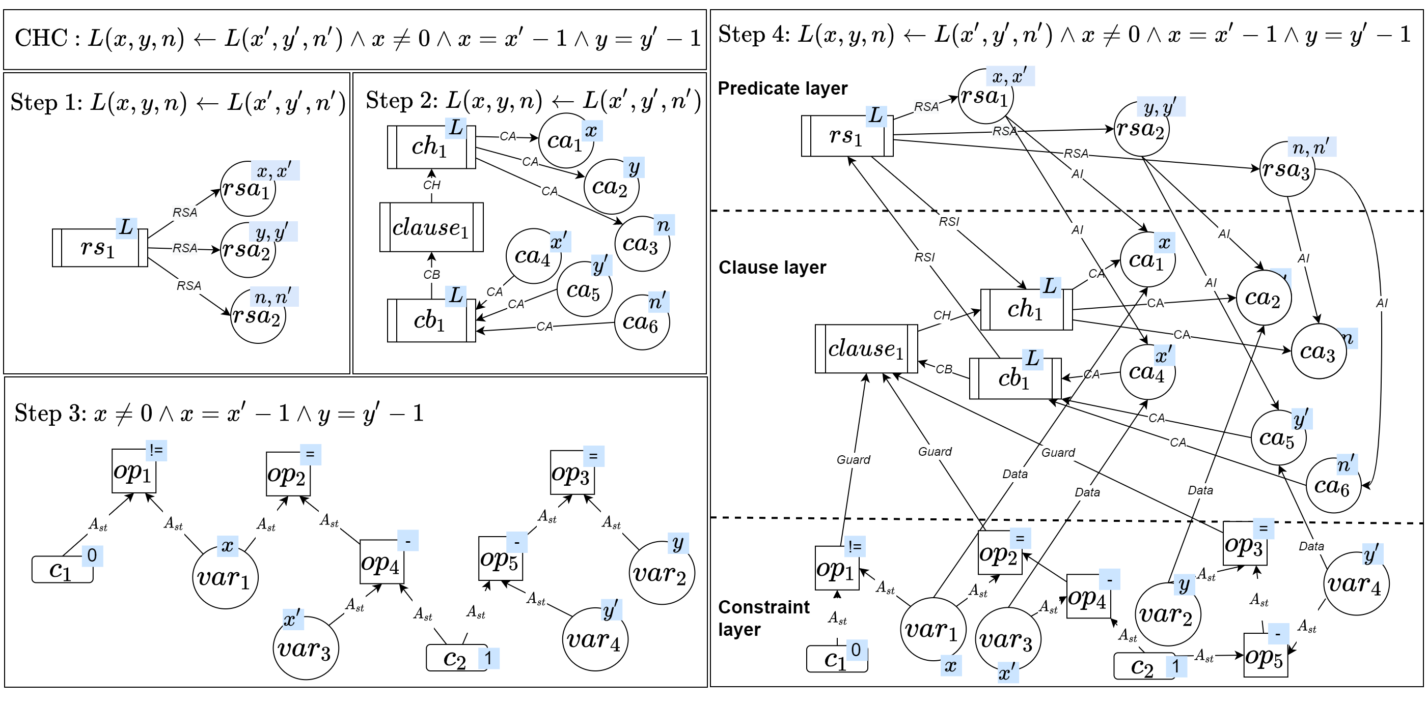
Figure 2: Construct constraint graph from the CHC $L(x,y,n)\leftarrow L(x^{\prime},y^{\prime},n^{\prime})\wedge x\neq 0\wedge x=x^{\prime}-1\wedge y=y^{\prime}-1$. Note that some nodes have multiple concrete symbol names (e.g., node $rsa_{1}$ has two concrete names, $x$ and $x^{\prime}$) since one relation symbol may bind with different arguments.

Formal definition of constraint graph .

A constraint graph $CG=(V,\mathit{BE},R^{CG},X^{CG},\ell)$ consists of a set of nodes $v\in V$, a set of typed binary edges $\mathit{BE}\in V\times V\times R^{CG}$, a set of edge types $r\in R^{CG}$ (Table 3), a set of node types $x\in X^{CG}$ (Table 2), and a map $\ell:v\rightarrow x$. Here, $(v_{1},v_{2},r)\in\mathit{BE}$ denotes a binary edge with edge type $r$. The node types are used to generate the initial feature $x_{v}$, a real-valued vector in R-HyGNN.

Table 2: Node types for constraint graph. The shape corresponds to the shape of nodes in Figure 2 and is only used for visualizing the example.

Node types $X^{CG}$	Layer	Explanation	Elements in CHCs	Shape
relation symbol ($rs$)	Predicate layer	Relation symbols in head or body	$L$
false	Predicate layer	false state	false
relation symbol argument ($rsa$)	Predicate layer	Arguments of the relation symbols	x, y
clause ($cla$)	Clause layer	Represent clause as a abstract node	$\emptyset$
clause head ($ch$)	Clause layer	Relation symbol in head	$L$
clause body ($cb$)	Clause layer	Relation symbol in body	$L$
clause argument ($ca$)	Clause layer	Arguments of relation symbol in head and body	$x,y$
variable ($var$)	Constraint layer	Free variables	n
operator ($op$)	Constraint layer	Operators over a theory	=, -
constant ($c$)	Constraint layer	Constants over a theory	0, 1, true

Table 3: Edge types for constraint graph. Here, $rs,rsa,cla$, etc. are node types described in Table 2.Here, “$|$" means “or". For example, $c~{}|~{}op~{}|var$ means this node could be node with type $c$, $op$, or $var$.

Edge type $R^{CG}$	Layer	Definition	Explanation
Relation Symbol Argument (RSA)	Predicate layer	($rs,rsa,\textit{RSA}$)	Connects relation symbols and their arguments
Relation Symbol Instance (RSI)	Between predicate and clause layer	$(rs,ch,\textit{RSA})~{}|~{}(cb,rs,\textit{RSA})$	Connects relation symbols with their head and body
Argument Instance (AI)	Between predicate and clause layer	($pa,ca,\textit{AI}$)	Connects relation symbols and their arguments
Clause Head (CH)	Clause layer	$(cla,ch,\textit{CH})$	Connect $clause$ node to its head
Clause Body (CB)	Clause layer	$(cb,cla,\textit{CB})$	Connect the $clause$ node to its body
Clause Argument (CA)	Clause layer	$(ca,cb,\textit{CA})~{}|~{}(ch,ca,\textit{CA})$	Connect $ch$ or $cb$ nodes with corresponding $ca$ nodes
Guard (GUARD)	Between clause and constraint layer	$(c~{}|~{}op,cla,\textit{GUARD})$	Connect the root node of the AST to corresponding $clause$ node
Data (DATA)	Between clause and constraint layer	$(var,ca,\textit{DATA})$	Connect $ca$ nodes to corresponding $var$ nodes AST
AST sub-term ($A_{st}$)	Constraint layer	$(c~{}|~{}var~{}|~{}op,op,A_{st})$	Connect nodes within AST

An abstract example of constraint graph .

Except for the concrete example, we give a abstract example to describe how to construct the constraint graph. First, the CHC $H\leftarrow B_{1}\wedge\cdots\wedge B_{n}\wedge\varphi$ in Section 2 can be re-written to

$$q_{1}(\bar{t_{1}})\leftarrow q_{2}(\bar{t_{2}})\wedge\cdots\wedge q_{k}(\bar{t_{k}})\wedge\varphi_{1}\wedge\cdots\varphi_{n},(n,k\in\mathbb{N}),$$ (2)

where $\varphi_{1}\cdots\varphi_{k}$ are sub-formulas for constraint $\varphi$. Notice that since there is no normalization for the original CHCs, the same relation symbols can appear in both head and body (i.e., $q_{1},q_{2},\cdots,q_{k}$ may equal to each other).

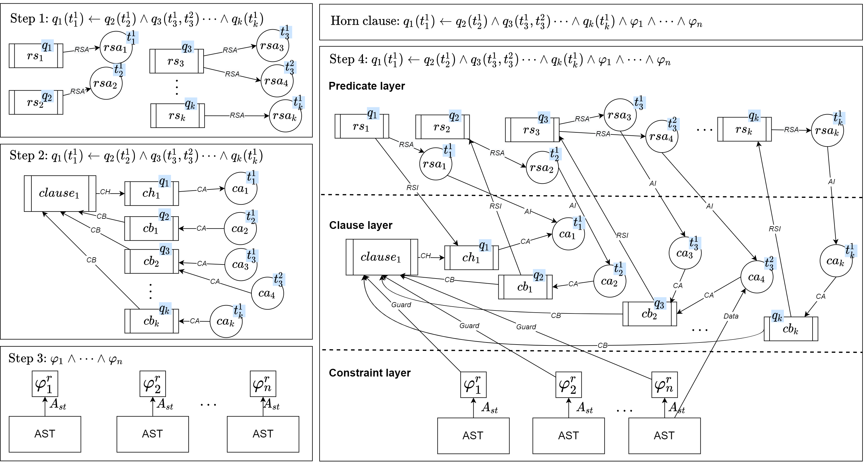
Figure 6: An example to illustrate how to construct the Constraint graph from the CHC in (3). Here, $\varphi_{i}^{r}$ is the AST root node $\varphi_{i}$.

Then, we can construct a constraint graph using Algorithm 1, in which the input is a set of CHC and the output is a constraint graph $CG=(V,\mathit{BE},R^{CG},X^{CG},\ell)$. The step-wise constructing process for the CHC in Eq. (2) is visualized in Figure 6.

3.2 Control- and Data-flow Hypergraph (CDHG)

In contrast to the constraint graph, the CDHG representation emphasizes the semantic information (control and data flow) in the CHCs by hyperedges which can join any number of vertices. To represent control and data flow in CDHG, first, we preprocess every CHC and then split the constraint into control and data flow sub-formulas.

Normalization.

We normalize every CHC by applying the following rewriting steps: (i) We ensure that every relation symbol occurs at most once in every clause. For instance, the CHC $q(a)\leftarrow q(b)\wedge q(c)$ has multiple occurrences of the relation symbol $q$, and we normalize it to equi-satisfiable CHCs $q(a)\leftarrow q^{\prime}(b)\wedge q^{\prime\prime}(c),q^{\prime}(b)\leftarrow q(b^{\prime})\wedge b=b^{\prime}$ and $q^{\prime\prime}(c)\leftarrow q(c^{\prime})\wedge c=c^{\prime}$. (ii) We associate each relation symbol $q$ with a unique vector of pair-wise distinct argument variables $\bar{x}_{q}$, and rewrite every occurrence of $q$ to the form $q(\bar{x}_{q})$. In addition, all the argument vectors $\bar{x}_{q}$ are kept disjoint. The normalized CHCs from Figure 1(c) are shown in Table 4.

Splitting constraints into control- and data-flow formulas.

We can rewrite the constraint $\varphi$ to a conjunction $\varphi=\varphi_{1}\wedge\cdots\wedge\varphi_{k},~{}k\in\mathbb{N}~{}.$ The sub-formula $\varphi_{i}$ is called a “data-flow sub-formula” if and only if it can be rewritten to the form $x=t(\bar{y})$ such that (i) $x$is one of the arguments in head $q(\bar{x}_{q})$; (ii) $t(\bar{y})$is a term over variables $\bar{y}$, where each element of $\bar{y}$ is an argument of some body literal $q^{\prime}(\bar{x}_{q^{\prime}})$. We call all other $\varphi_{j}$ “control-flow sub-formulas”. A constraint $\varphi$ can then be represented by $\varphi=g_{1}\wedge\cdots\wedge g_{m}\wedge d_{1}\wedge\cdots\wedge d_{n}$, where $m,n\in\mathbb{N}$ and $g_{i}$ and $d_{j}$ are the control- and data-flow sub-formulas, respectively. The control and data flow sub-formulas for the normalized CHCs of our running example are shown in Table 4.

Table 4: Control- and data-flow sub-formula in constraints for the normalized CHCs from Figure 1(c)

Normalized CHCs	Control-flow sub-formula	Data-flow sub-formula
$L(x,y,n)\leftarrow n\geq 0\wedge x=n\wedge y=n$	$n\geq 0$	$x=n,y=n$
$L(x,y,n)\leftarrow L^{\prime}(x^{\prime},y^{\prime},n^{\prime})\wedge x\neq 0\wedge x=x^{\prime}-1\wedge y=y^{\prime}-1$	$x\neq 0$	$x=x^{\prime}-1,y=y^{\prime}-1$
$L^{\prime}(x^{\prime},y^{\prime},n^{\prime})\leftarrow L(x,y,n)\wedge x^{\prime}=x\wedge y^{\prime}=y\wedge n^{\prime}=n$	empty	$x^{\prime}=x,y^{\prime}=y,n^{\prime}=n$
$\textit{false}\leftarrow L(x,y,n)\wedge x=0\wedge y\neq 0$	$y\neq 0$	$x=0$

Constructing a CDHG.

The CDHG represents program control- and data-flow by guarded control-flow hyperedges CFHE and data-flow hyperedges DFHE. A CFHE edge denotes the flow of control from the body to head literals of the CHC. A DFHE edge denotes how data flows from the body to the head. Both control- and data-flow are guarded by the control flow sub-formula.

Constructing the CDHG for a normalized CHC $L(x,y,n)\leftarrow L^{\prime}(x^{\prime},y^{\prime},n^{\prime})\wedge x\neq 0\wedge x=x^{\prime}-1\wedge y=y^{\prime}-1$ is shown in Figure 3. The corresponding node and edge types are described in Tables 5 and 6.

In the first step, we draw relation symbols and their arguments and build the relation between them. In the second step, we add a $guard$ node and draw ASTs for the control flow sub-formulas. In the third step, we construct guarded control-flow edges by connecting the relation symbols in the head and body and the $guard$ node, which connects the root of control flow sub-formulas. In the fourth step, we construct the ASTs for the right-hand side of every data flow sub-formula. In the fifth step, we construct the guarded data-flow edges by connecting the left- and right-hand sides of the data flow sub-formulas and the $guard$ node. Note that the diamond shapes in Figure 3 are not nodes in the graph but are used to visualize our (ternary) hyperedges of types CFHE and DFHE. We show it in this way to visualize CDHG better.

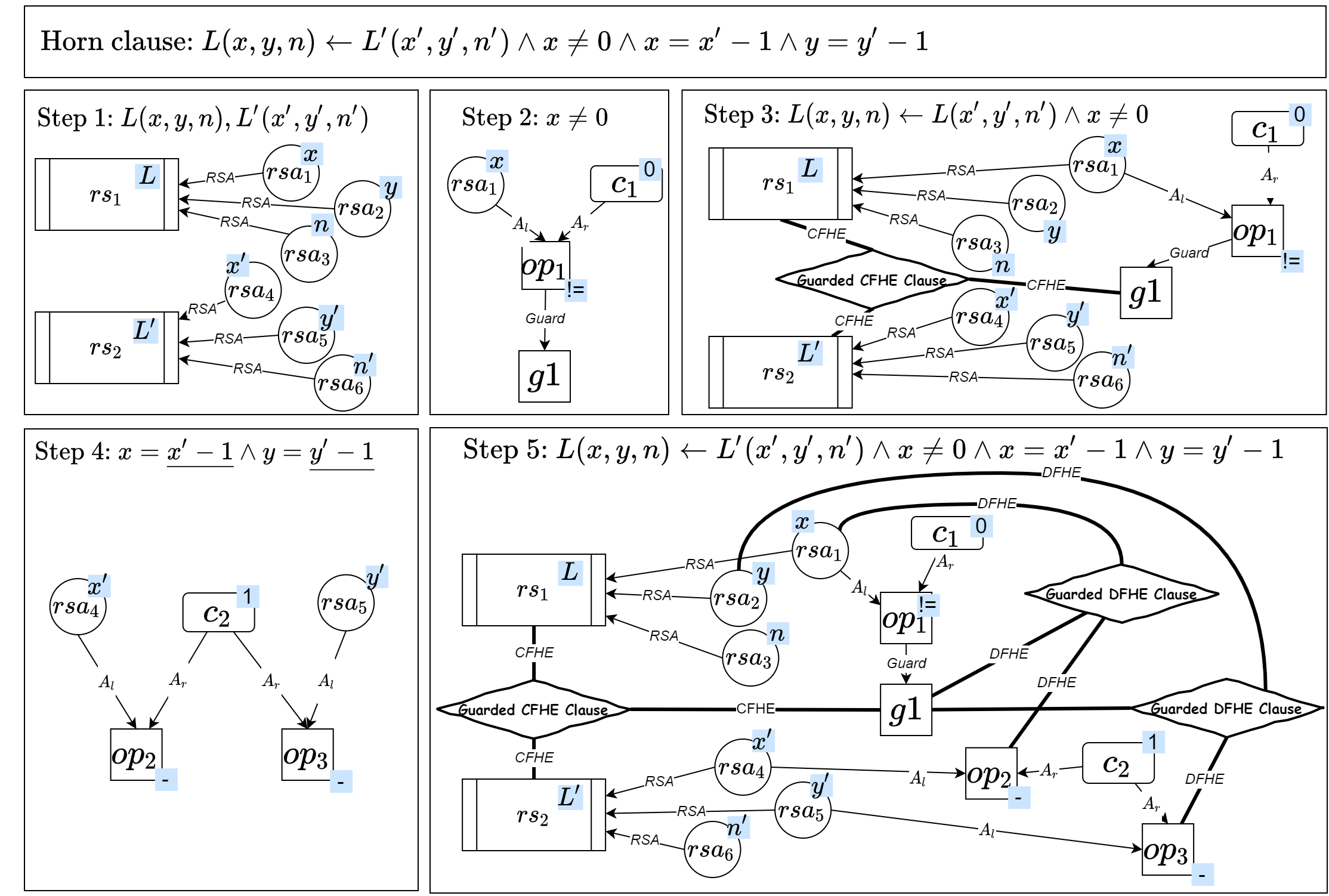
Figure 3: Construct the CDHG from the CHC $L(x,y,n)\leftarrow L^{\prime}(x^{\prime},y^{\prime},n^{\prime})\wedge x\neq 0\wedge x=x^{\prime}-1\wedge y=y^{\prime}-1$.

Formal definition of CDHG.

A CDHG $HG=(V,\mathit{HE},R^{CDHG},X^{CDHG},\ell)$ consists of a set of nodes $v\in V$, a set of typed hyperedge $\mathit{HE}\in V^{*}\times R^{CDHG}$ where $V^{*}$ is a list of node from $V$, a set of node types $x\in X^{CDHG}$ (Table 5),a set of edge types $r\in R^{CDHG}$ (Table 6), and a map $\ell:v\rightarrow x$. Here, $(v_{1},v_{2},\cdots,v_{n},r)\in HE$ denotes a hyperedge for a list of nodes $(v_{1},\cdots,v_{n})$ with edge type $r$. The node types are used to generate the initial feature $x_{v}$, a real-valued vector, in R-HyGNN.

The guarded CFHE is a typed hyperedge $(v_{1},\cdots,v_{n},g,\textit{CFHE})\in\textit{HE}$, where the type of $v_{1},\cdots,v_{n}$ is $rs$. Since R-HyGNN has more stable performance with fixed number of node in one edge type, we transform the hyperedge $(v_{1},\cdots,v_{n},g,\mathit{CFHE})\in HE$ with variable number of nodes to a set of ternary hyperedges (i.e., $\{(v_{1},v_{2},g,$ $\mathit{CFHE}),(v_{1},v_{3},g,\mathit{CFHE}),\cdots,(v_{1},v_{n},g,\mathit{CFHE})\}$).

The guarded DFHE is a typed ternary hyperedge $(v_{i},v_{j},g,\mathit{DFHE})\in\mathit{HE}$, where $v_{i}$’s type is $rsa$ and $v_{j}$’s type could be one of $\{op,c,v\}$.

Table 5: Node types for the CDHG. Note that Tables 2 and 5 use some same node types because they represent the same elements in the CHC. Some abstract nodes, such as initial and guard, do not have concrete symbol names since they do not directly associate with any element in the CHCs.

Node types $X^{CDHG}$	Explanation	Elements in CHCs	Shape
relation symbol ($rs$)	Relation symbols in head or body	$L$
initial	Initial state	$\emptyset$
false	false state	false
relation symbol argument ($rsa$)	Arguments of the relation symbols	$x,y$
variables ($var$)	Free variables	$n$
operator ($op$)	Operators over a theory	=, +
constant ($c$)	Constant over a theory	0, 1, $true$
guard ($g$)	Guard for CFHE and DFHE	$\emptyset$

Table 6: Edge types for the CDHG. $rs,rsa,var,op,c,etc.$ are node types from Table 5.

Edge type $R^{CDHG}$	Edge arity	Definition	Explanation
Control Flow Hyperedge (CFHE)	Ternary	$(rs_{1},rs_{2}~{}|~{}\textit{false},g,$ $\textit{CFHE})$	Connects the $rs$ node in body and head, and abstract guard node
Data Flow Hyperedge (DFHE)	Ternary	$(a,op~{}|~{}c~{}|~{}var,g,\textit{DFHE})$	Connects the root node of right-hand and left-hand side of data flow sub-formulas, and a abstract guard node
Guard (Guard)	Binary	$(op~{}|~{}c,g,\textit{Guard})$	Connects all roots of ASTs of control flow sub-formulas and the $guard$ node
Relation Symbol Argument (RSA)	Binary	$(a,rs,\textit{RSA})$	Connects $rsa$ nodes and their $rs$ node
AST_left ($A_{l}$)	Binary	$(op,op~{}|~{}var~{}|~{}c,A_{l})$	Connects left-hand side element of a binary operator or an element from a unary operator
AST_right ($A_{r}$)	Binary	$(op,op~{}|~{}var~{}|~{}c,A_{r})$	It connects right-hand side element of a binary operator

An abstract example of CDHG.

Except for the concrete example, we give a abstract example to describe how to construct the CDHG. After the preprocessings (normalization and splitting the constraint to guard and data flow sub-formulas), the CHC $H\leftarrow B_{1}\wedge\cdots\wedge B_{n}\wedge\varphi$ in Section 2 can be re-written to

$$q_{1}(\bar{t_{1}})\leftarrow q_{2}(\bar{t_{2}})\wedge\cdots\wedge q_{k}(\bar{t_{k}})\wedge g_{1}\wedge\cdots g_{m}\wedge d_{1}\wedge\cdots d_{n},(m,n,k\in\mathbb{N}).$$ (3)

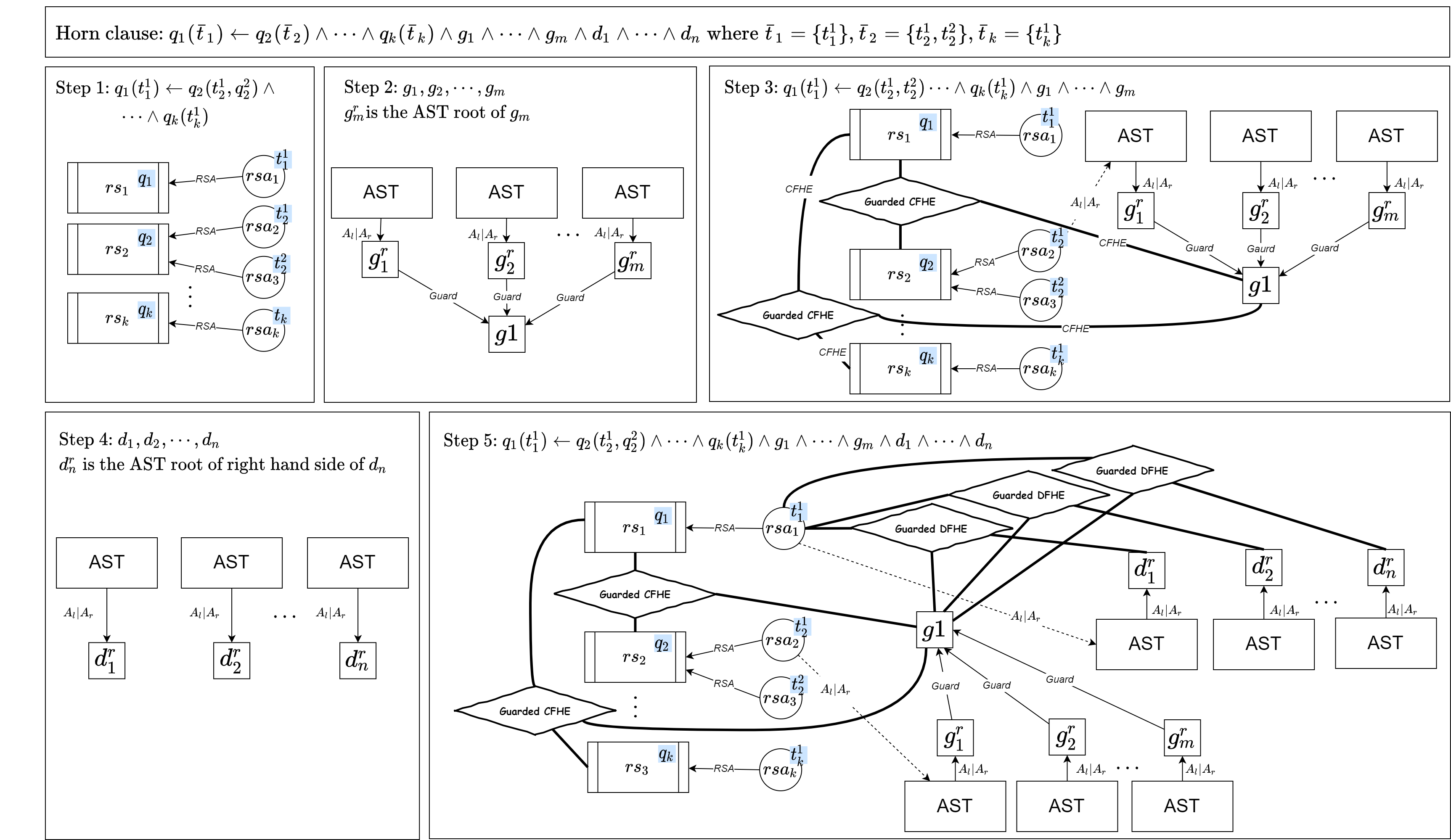
Figure 7: An example to illustrate how to construct the CDHG from the CHC in (3). Here, $g_{i}^{r}$ and $d_{j}^{r}$ are the AST root node of control flow sub-formula $g_{i}$ and the right-hand side of the data flow sub-formula, respectively. The “$|$" connected edge type $A_{l}~{}|~{}A_{r}$ means the edge could be type $A_{l}$ or $A_{r}$.

We can construct the corresponding CDHG using Algorithm 2, in which the input is a set of CHC and the output is a CDHG $HG=(V,\mathit{HE},R^{CDHG},X^{CDHG},\ell)$. The step-wise constructing process for the CHC in (3) is visualized in Figure 7.

4 Relational Hypergraph Neural Network

Different from regular graphs, which connect nodes by binary edges, CDHG includes hyperedges which connect arbitrary number of nodes. Therefore, we extend R-GCN to R-HyGNN to handle hypergraphs. Concretely, to compute a new representation of a node $v$ at timestep $t$, we consider all hyperedges $e$ that involve $v$. For each such hyperedge we create a “message” by concatenating the representations of all nodes involved in that hyperedge and multiplying the result with a learnable matrix $W_{r,p}^{t}$, where $r$ is the type of the relation and $p$ the position that $v$ takes in the hyperedge. Intuitively, this means that we have one learnable matrix for each distinguishable way a node can be involved in a relation. Hence, the updating rule for node representation at time step $t$ in R-HyGNN is

$$h_{v}^{t}={\rm ReLU}(\sum_{r\in R}\sum_{p\in P_{r}}\sum_{e\in E_{v}^{r,p}}W_{r,p}^{t}\cdot\|[h_{u}^{t-1}\mid u\in e]),$$ (4)

where $\|\{\cdot\}$ denotes concatenation of all elements in a set, $r\in R=\{r_{i}\mid i\in\mathbb{N}\}$ is the set of edge types (relations), $p\in P_{r}=\{p_{j}\mid j\in\mathbb{N}\}$ is the set of node positions under edge type $r$, $W_{r,p}^{t}$ denotes learnable parameters when the node is in the $p$th position with edge type $r$, and $e\in E_{v}^{r,p}$ is the set of hyperedges of type $r$ in the graph in which node $v$ appears in position $p$, where $e$ is a list of nodes. The updating process for the representation of node $v$ at time step 1 is illustrated in Figure 4.

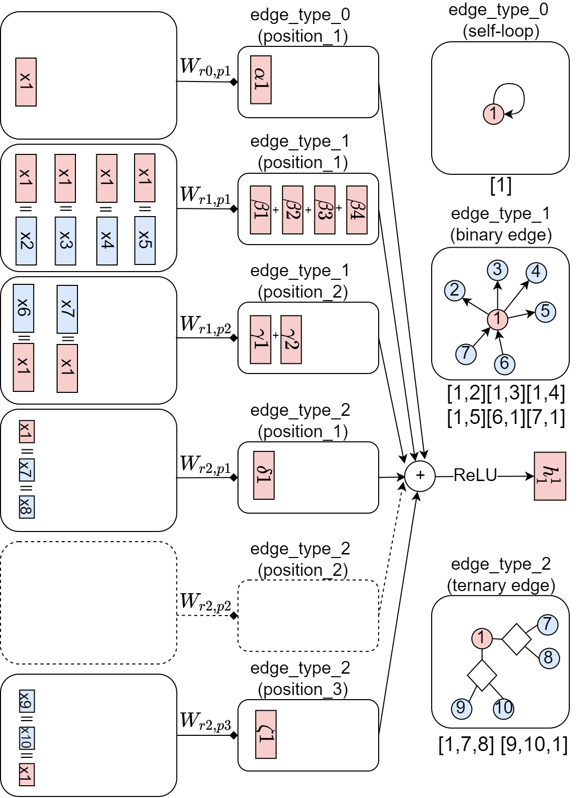
Figure 4: An example to illustrate how to update node representation for R-HyGNN using (4). At the right-hand side, there are three types of edges connected with node 1. We compute the updated representation $h_{1}^{1}$ for node 1 at the time step 1. $\|$ means concatenation. $x_{i}$ is the initial feature vector of node $i$. The red blocks are the trace of the updating for node 1. The edge type 1 is a unary edge and is a self-loop. It has one set of learnable parameters as the update function i.e., $W_{r0,p1}$. The edge type 2 is binary edge, it has two update functions i.e., $W_{r1,p1}$ and $W_{r1,p2}$. Node 1 is in the first position in edge [1,2], [1,3], [1,4], and [1,5], so the concatenated node representation will be updated by $W_{r1,p1}$ . On the other hand, for the other two edges [6,1] and [7,1], node 1 is in the second position, so the concatenated node representation will be updated by $W_{r1,p2}$. For edge type 3, the same rule applies, i.e., depending on node 1’s position in the edge, the concatenated node representation will go through different parameter sets. Since there is no edge that node 1 is in the second position, we use a dashed box and arrow to represent it. The aggregation is to add all updated representations from different edge types.

Note that different edge types may have the same number of connected nodes. For instance, in CDHG, CFHE and DFHE are both ternary edges.

Overall, our definition of R-HyGNN is a generalization of R-GCN. Concretely, it can directly be applied to the special-case of binary graphs, and in that setting is slightly more powerful as each message between nodes is computed using the representations of both source and target nodes, whereas R-GCN only uses the source node representation.

4.1 Training Model

The end-to-end model consists of three components: the first component is an embedding layer, which learns to map the node’s type (encoded by integers) to the initial feature vectors; the second component is R-HyGNN, which learns program features; the third component is a set of fully connected neural networks, which learns to solve a specific task by using gathered node representations from R-HyGNNs. All parameters in these three components are trained together. Note that different tasks may gather different node representations. For example, Task 1 gathers all node representations, while Task 2 only gathers node representations with type $rs$.

We set all vector lengths to 64, i.e., the embedding layer output size, the middle layers’ neuron size in R-HyGNNs, and the layer sizes in fully connected neural networks are all 64. The maximum training epoch is 500, and the patient is 100. The number of message passing steps is 8 (i.e., (4) is applied eight times). For the rest of the parameters (e.g., learning rate, optimizer, dropout rate, etc.), we use the default setting in the tf2_gnn framework. We set these parameters empirically according to the graph size and the structure. We apply these fixed parameter settings for all tasks and two graph representations without fine-tuning.

5 Proxy Tasks

We propose five proxy tasks with increasing difficulty to systematically evaluate the R-HyGNN on the two graph representations. Tasks 1 to 3 evaluate if R-HyGNN can solve general problems in graphs. In contrast, Tasks 4 and 5 evaluate if combining our graph representations and R-HyGNN can learn program features to solve the encoded program verification problems. We first describe the learning target for every task and then explain how to produce training labels and discuss the learning difficulty.

Task 1: Argument identification.

For both graph representations, the R-HyGNN model performs binary classification on all nodes to predict if the node type is a relation symbol argument ($rsa$) and the metric is accuracy. The binary training label is obtained by reading explicit node types. This task evaluates if R-HyGNN can differentiate explicit node types. This task is easy because the graph explicitly includes the node type information in both typed nodes and edges.

Task 2: Count occurrence of relation symbols in all clauses.

For both graph representations, the R-HyGNN model performs regression on nodes with type $rs$ to predict how many times the relation symbols occur in all clauses. The metric is mean square error. The training label is obtained by counting the occurrence of every relation symbol in all clauses. This task is designed to see if R-HyGNN can correctly perform a counting task. For example, the relation symbol $L$ occurs four times in all CHCs in Figure 4, so the training label for node $L$ is value 4. This task is harder than Task 1 since it needs to count the connected binary edges or hyperedges for a particular node.

Task 3: Relation symbol occurrence in SCCs.

For both graph representations, the R-HyGNN model performs binary classification on nodes with type $rs$ to predict if this node is an SCC (i.e., in a cycle) and the metric is accuracy. The binary training label is obtained using Tarjan’s algorithm [19]. For example, in Figure 4, $L$ is an SCC because $L$ and $L^{\prime}$ construct a cycle by $L\leftarrow L^{\prime}$ and $L^{\prime}\leftarrow L$. This task is designed to evaluate if R-HyGNN can recognize general graph structures such as cycles. This task requires the model to classify a graph-theoretic object (SCC), which is harder than the previous two tasks since it needs to approximate a concrete algorithm rather than classifying or counting explicit graphical elements.

Task 4: Existence of argument bounds.

For both graph representations, we train two independent R-HyGNN models which perform binary classification on nodes with type $rsa$ to predict if individual arguments have (a) lower and (b) upper bounds in the least solution of a set of CHCs, and the metric is accuracy. To obtain the training label, we apply the Horn solver Eldarica to check the correctness of guessed (and successively increased) lower and upper arguments bounds; arguments for which no bounds can be shown are assumed to be unbounded. We use a timeout of 3 s for the lower and upper bound of a single argument, respectively. The overall timeout for extracting labels from one program is 3 hours. For example, consider the CHCs in Fig. 1(c). The CHCs contain a single relation symbol $L$; all three arguments of $L$ are bounded from below but not from above. This task is (significantly) harder than the previous three tasks, as boundedness of arguments is an undecidable property that can, in practice, be approximated using static analysis methods.

Task 5: Clause occurrence in counter-examples

This task consists of two binary classification tasks on nodes with type guard (for CDHG), and with type clause (for constraint graph) to predict if a clause occurs in the counter-examples. Those kinds of nodes are unique representatives of the individual clauses of a problem. The task focuses on unsatisfiable sets of CHCs. Every unsatisfiable clause set gives rise to a set of minimal unsatisfiable subsets (MUSes); MUSes correspond to the minimal CEs of the clause set. Two models are trained independently to predict whether a clause belongs to (a) the intersection or (b) the union of the MUSes of a clause set. The metric for this task is accuracy. We obtain training data by applying the Horn solver Eldarica [25], in combination with an optimization library that provides an algorithm to compute MUSes. This task is hard, as it attempts the prediction of an uncomputable binary labelling of the graph.

6 Evaluation

We first describe the dataset we use for the training and evaluation and then analyse the experiment results for the five proxy tasks.

6.1 Benchmarks and Dataset

Table 7 shows the number of labelled graph representations from a collection of CHC-COMP benchmarks [20]. All graphs were constructed by first running the preprocessor of Eldarica [25] on the clauses, then building the graphs as described in Section 3, and computing training data. For instance, in the first four tasks we constructed 2337 constraint graphs with labels from 8705 benchmarks in the CHC-COMP LIA-Lin track (linear Horn clauses over linear integer arithmetic). The remaining 6368 benchmarks are not included in the learning dataset because when we construct the graphs, (1) the data generation process timed out, or (2) the graphs were too big (more than 10,000 nodes), or (3) there was no clause left after simplification. In Task 5, since the label is mined from CEs, we first need to identify unsat benchmarks using a Horn solver (1-hour timeout), and then construct graph representations. We obtain 881 and 857 constraint graphs when we form the labels for Task 5 (a) and (b), respectively, in LIA-Lin.

Finally, to compare the performance of the two graph representations, we align the dataset for both two graph representations to have 5602 labelled graphs for the first four tasks. For Task 5 (a) and (b), we have 1927 and 1914 labelled graphs, respectively. We divide them to train, valid, and test sets with ratios of 60%, 20%, and 20%. We include all corresponding files for the dataset in a Github repository .

Table 7: The number of labeled graph representations extracted from a collection of CHC-COMP benchmark  [20]. For each SMT-LIB file, the graph representations for Task 1,2,3,4 are extracted together using the timeout of 3 hours, and for task 5 is extracted using 20 minutes timeout. Here, T. denotes Task.

	SMT-LIB files		Constraint graphs			CDHGs
	Total	Unsat	T. 1-4	T. 5 (a)	T. 5 (b)	T. 1-4	T. 5 (a)	T. 5 (b)
Linear LIA	8705	1659	2337	881	857	3029	880	883
Non-linear LIA	8425	3601	3376	1141	1138	4343	1497	1500
Aligned	17130	5260	5602	1927	1914	5602	1927	1914

6.2 Experimental Results for Five Proxy Tasks

From Table 8, we can see that for all binary classification tasks, the accuracy for both graph representations is higher than the ratios of the dominant labels. For the regression task, the scattered points are close to the diagonal line. These results show that R-HyGNN can learn the syntactic and semantic information for the tasks rather than performing simple strategies (e.g., fill all likelihood by 0 or 1). Next, we analyse the experimental results for every task.

Task 1: Argument identification.

When the task is performed in the constraint graph, the accuracy of prediction is 100%, which means R-HyGNN can perfectly differentiate if a node is a relation symbol argument $rsa$ node. When the task is performed in CDHG, the accuracy is close to 100% because, unlike in the constraint graph, the number of incoming and outgoing edges are fixed (i.e., $RSA$ and $AI$), the $rsa$ nodes in CDHG may connect with a various number of edges (including $RSA$, $AST\_1$, $AST\_2$, and DFHE) which makes R-HyGNN hard to predict the label precisely.

Besides, the data distribution looks very different between the two graph representations because the normalization of CHCs introduces new clauses and arguments. For example, in the simplified CHCs in Figure 1(c), there are three arguments for the relation symbol $L$, while in the normalized clauses in Figure 4, there are six arguments for two relation symbols $L$ and $L^{\prime}$. If the relation symbols have a large number of arguments, the difference in data distribution between the two graph representations becomes larger. Even though the predicted label in this task cannot directly help solve the CHC-encoded problem, it is important to study the message flows in the R-HyGNNs.

Task 2: Count occurrence of relation symbols in all clauses.

In the scattered plots in Figure 5, the x- and y-axis denote true and the predicted values in the logarithm scale, respectively. The closer scattered points are to the diagonal line, the better performance of predicting the number of relation symbol occurrences in CHCs. Both CDHG and constraint graph show good performance (i.e., most of the scattered points are near the diagonal lines). This syntactic information can be obtained by counting the CFHE and RSI edges for CDHG and constraint graph, respectively. When the number of nodes is large, the predicted values are less accurate. We believe this is because graphs with a large number of nodes have a more complex structure, and there is less training data. Moreover, the mean square error for the CDHG is larger than the constraint graph because normalization increases the number of nodes and the maximum counting of relation symbols for CDHG, and the larger range of the value is, the more difficult for regression task. Notice that the number of test data (1115) for this task is less than the data in the test set (1121) shown in Table 7 because the remaining six graphs do not have a $rs$ node.

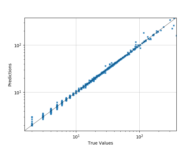
(a) Scatter plot for CDHG. The total $rs$ node number is 16858. The mean square error is 4.22.

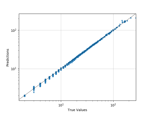
(b) Scatter plot for constraint graph. The total $rs$ node number is 11131. The mean square error is 1.04.

Figure 5: Scatter plot for Task 2. The x- and y-axis are in logarithmic scales.

Task 3: Relation symbol occurrence in SCCs.

The predicted high accuracy for both graph representations shows that our framework can approximate Tarjan’s algorithm [19]. In contrast to Task 2, even if the CDHG has more nodes than the constraint graph on average, the CDHG has better performance than the constraint graph , which means the control and data flow in CDHG can help R-HyGNN to learn graph structures better. For the same reason as task 2, the number of test data (1115) for this task is less than the data in the test set (1121).

Task 4: Existence of argument bounds.

For both graph representations, the accuracy is much higher than the ratio of the dominant label. Our framework can predict the answer for undecidable problems with high accuracy, which shows the potential for guiding CHC solvers. The CDHG has better performance than the constraint graph, which might be because predicting argument bounds relies on semantic information. The number of test data (1028) for this task is less than the data in the test set (1121) because the remaining 93 graphs do not have a $rsa$ node.

Task 5: Clause occurrence in counter-examples.

For Task (a) and (b), the overall accuracy for two graph representations is high. We manually analysed some predicted results by visualizing the (small) graphs. We identify some simple patterns that are learned by R-HyGNNs. For instance, the predicted likelihoods are always high for the $rs$ nodes connected to the $\mathit{false}$ nodes. One promising result is that the model can predict all labels perfectly for some big graphs that contain more than 290 clauses, which confirms that the R-HyGNN is learning certain intricate patterns rather than simple patterns. In addition, the CDHG has better performance than the constraint graph , possibly because semantic information is more important for solving this task.

Table 8: Experiment results for Tasks 1,3,4,5. Both the fourth and fifth tasks consist of two independent binary classification tasks. Here, $+$ and $-$ stands for the positive and negative label. The T and P represent the true and predicted labels. The Acc. is the accuracy of binary classifications. The Dom. is dominant label ratio. Notice that even if the two graph representations originate from the same original CHCs, the label distributions are different since the CDHG is constructed from normalized CHCs.

			CG				CDHG
Task	Files		+	-	Acc.	Dom.	+	-	Acc.	Dom.
1	1121	+	93863	0	100%	95.1%	142598	0	99.9%	72.8%
		-	0	1835971			10	381445
3	1115	+	3204	133	96.1%	70.1%	8262	58	99.6%	50.7%
		-	301	7493			15	8523
4 (a)	1028	+	13685	5264	91.2%	79.7%	30845	4557	94.3%	75.2%
		-	2928	71986			3566	103630
4 (b)		+	18888	4792	91.4%	74.8%	41539	4360	94.3%	67.8%
		-	3291	66892			3715	92984
5 (a)	386	+	1048	281	95.0%	84.7%	1230	206	96.9%	86.4%
		-	154	7163			121	9036
5 (b)	383	+	3030	558	84.6%	53.1%	3383	481	90.6%	54.8%
		-	622	3428			323	4361

7 Related Work

Learning to represent programs.

Contextual embedding methods (e.g. transformer [28], BERT [29], GPT [30], etc.) achieved impressive results in understanding natural languages. Some methods are adapted to explore source code understanding in text format (e.g. CodeBERT [31], cuBERT [32], etc.). But, the programming language usually contains rich, explicit, and complicated structural information, and the problem sets (learning targets) of it [33, 34] are different from natural languages. Therefore, the way of representing the programs and learning models should adapt to the programs’ characteristics. Recently, the frameworks consisting of structural program representations (graph or AST) and graph or tree-based deep learning models made good progress in solving program language-related problems. For example, [35] represents the program by a sequence of code subtokens and predicts source code snippets summarization by a novel convolutional attention network. Code2vec [36] learns the program from the paths in its AST and predicts semantic properties for the program using a path-based attention model. [37] use AST to represent the program and classify programs according to functionality using the tree-based convolutional neural network (TBCNN). Some studies focus on defining efficient program representations, others focus on introducing novel learning structures, while we do both of them (i.e. represent the CHC-encoded programs by two graph representations and propose a novel GNN structure to learn the graph representations).

Deep learning for logic formulas.

Since deep learning is introduced to learn the features from logic formulas, an increasing number of studies have begun to explore graph representations for logic formulas and corresponding learning frameworks because logic formulas are also highly structured like program languages. For instance, DeepMath [38] had an early attempt to use text-level learning on logic formulas to guide the formal method’s search process, in which neural sequence models are used to select premises for automated theorem prover (ATP). Later on, FormulaNet [39] used an edge-order-preserving embedding method to capture the structural information of higher-order logic (HOL) formulas represented in a graph format. As an extension of FormulaNet, [40] construct syntax trees of HOL formulas as structural inputs and use message-passing GNNs to learn features of HOL to guide theorem proving by predicting tactics and tactic arguments at every step of the proof. LERNA [41] uses convolutional neural networks (CNNs) [42] to learn previous proof search attempts (logic formulas) represented by graphs to guide the current proof search for ATP. NeuroSAT [43, 44] reads SAT queries (logic formulas) as graphs and learns the features using different graph embedding strategies (e.g. message passing GNNs) [45, 46, 26]) to directly predict the satisfiability or guide the SAT solver. Following this trend, we introduce R-HyGNN to learn the program features from the graph representation of CHCs.

Graph neural networks.

Message passing GNNs [26], such as graph convolutional network (GCN) [17], graph attention network (GAT) [47], and gated graph neural network (GGNN) [46] have been applied in several domains ranging from predicting molecule properties to learning logic formula representations. However, these frameworks only apply to graphs with binary edges. Some spectral methods have been proposed to deal with the hypergraph [48, 49]. For instance, the hypergraph neural network (HGNN) [50] extends GCN proposed by [51] to handle hyperedges. The authors in [52] integrate graph attention mechanism [47] to hypergraph convolution [51] to further improve the performance. But, they cannot be directly applied to the spatial domain. Similar to the fixed arity predicates strategy described in LambdaNet [18], R-HyGNN concatenates node representations connected by the hyperedge and updates the representation depending on the node’s position in the hyperedge.

8 Conclusion and Future Work

In this work, we systematically explore learning program features from CHCs using R-HyGNN, using two tailor-made graph representations of CHCs. We use five proxy tasks to evaluate the framework. The experimental results indicate that our framework has the potential to guide CHC solvers analysing Horn clauses. In future work, among others we plan to use this framework to filter predicates in Horn solvers applying the CEGAR model checking algorithm.

Input: Simplified CHCs $\Pi$

Output: A constraint graph $\textit{CG}=(V,\textit{BE},R^{CG},X^{CG},\ell)$

Initialise graph: $V,\textit{BE},\ell=\emptyset,\emptyset,\emptyset$;

for  each clause $C$ in $\Pi$ do

       //step 1: construct the predicate layer;

       for  each relation symbol $q(\bar{t})$ in $C$  do

             if $v_{q}\notin V$ then

                   //construct a $rs$ node;

                   add a node $v_{q}$ with type $rs$ to $V$. Update map $\ell$; //construct $rsa$ nodes and connect them to the $rs$ node;

                   for  each argument $t$ in $\bar{t}$ do

                         add a node $v_{q}^{t}$ with type $rsa$ to $V$. Update map $\ell$;

                         add a edge from $v_{q}$ to $v_{q}^{t}$ to with type RSA to BE ; 

                   end for

                  

             end if

            

       end for

      //step 2: construct the clause layer;

       add a node $v_{clause}$ with type $clause$ to $V$. Update map $\ell$; add a clause head node $v_{q}^{h}$ with type $ch$ to $V$ for the relation symbol in $C$’ head. Update map $\ell$;

       add a edge from $v_{clause}$ to $v_{q}^{h}$ with type CH to BE ;

       for  each argument $t$ in $\bar{t}$  do

             add a node $v_{q}^{h,t}$ with type $ca$ to $V$. Update map $\ell$;

             add a edge from $v_{q}^{h}$ to $v_{q}^{h,t}$ with type CA to BE ;

            

       end for

      for  each relation symbol $q(\bar{t})$ in $C$’ body  do

             add a clause body node $v_{q}^{b}$ with type $cb$ to $V$. Update map $\ell$ ;

             add a edge from $v_{q}^{b}$ to $v_{clause}$ to with type CB to BE ;

             for  each argument $t$ in $\bar{t}$  do

                   add a node $v_{q}^{b,t}$ with type $ca$ to $V$. Update map $\ell$;

                   add a edge from $v_{q}^{b,t}$ to $v_{q}^{t}$ to with type CA to BE ;

                  

             end for

            

       end for

      //step 3: construct the constraint layer;

       for  each sub-expression $\phi_{i}$ in the constraint do

             for  each sub-expressions $se$ in $\phi_{i}$  do

                   if $v_{se}\notin V$ then

                         add a node $v_{se}$ with type $rsa,var,c$ or $op$ to $V$. Update map $\ell$;

                        

                   end if

                  add edge from $v_{se}$ to the left and right child of $se$ to BE with type $A_{st}$;

                  

             end for

            

       end for

      //step 4: add connection between three layers;

       for  each relation symbol node $v_{q}$ in predicate layer with type $rs$  do

             add edge $(v_{q},v_{q}^{h})$ or $(v_{q}^{b},v_{q})$ to $\mathit{BE}$ with type $RSI$;

            

       end for

      for  each argument node $v_{q}^{t}$ in predicate layer with type $rsa$  do

             add edge $(v_{q}^{t},v_{q}^{h,t})$ or $(v_{q}^{b,t},v_{q}^{t})$ to BE with type $AI$;

            

       end for

      for  each root node of sub-expression $v_{\phi_{i}^{r}}$  do

             add edge $(v_{\phi_{i}^{r}},v_{clause})$ to BE with type Guard;

            

       end for

      for  each node $v_{se}$ in AST tree with type $v$; if $v_{se}$ is an argument node  do

             add edge $(v_{se},v_{q}^{h,t})$ or $(v_{q}^{b,t},v_{se})$ to BE with type Data;

            

       end for

      

end for

return $V,\textit{HE},\ell$

Algorithm 1 Construct a constraint graph from CHCs

Input: Normalized CHCs $\Pi$

Output: A CDHG $\mathit{HG}=(V,\textit{HE},R^{CDHG},X^{CDHG},\ell)$

Initialise graph: $V,\textit{HE},\ell=\emptyset,\emptyset,\emptyset$;

for  each clause $C$ in $\Pi$ do

       Add node $v_{initial}$ and $v_{\mathit{false}}$ with type initial and $\mathit{false}$ to $V$. Update map $\ell$;

       //step 1: construct relation symbols and their arguments as typed nodes and add the $RSA$ edge between them;

       for  each relation symbol $q(\bar{t})$ in $C$  do

             if $v_{q}\notin V$ then

                   add a node $v_{q}$ with type $rs$ to $V$. Update map $\ell$;

                   for  each argument $t$ in $\bar{t}$  do

                         add a node $v_{q}^{t}$ with type $rsa$ to $V$. Update map $\ell$;

                         add a edge from $v_{q}$ to $v_{q}^{t}$ to with type RSA to HE ; 

                   end for

                  

             end if

            

       end for

      //step 2: construct ASTs for control flow sub-formulas in the constraints and connects the roots of ASTs to an abstract node with type Guard;

       add a node $v_{g}$ with type $guard$ to $V$. Update map $\ell$; for  each $g_{i}$  do

             for  each sub-expression $se$ in $g_{i}$  do

                   if $v_{se}\notin V$ then

                         add a node $v_{se}$ with type $rsa,var,c,$ or $op$ to $V$. Update map $\ell$;

                        

                   end if

                  add edge from $v_{se}$ to left and right child of $se$ to $\mathit{HE}$ with type $A_{l}$ and $A_{r}$, respectively;

                  

             end for

            add edge from $g_{i}^{r}$ to $v_{g}$ with type Guard to $\mathit{HE}$, where $g_{i}^{r}$ is the root node of $g_{i}$’s AST;

            

       end for

      //step 3: construct CFHEs;

       if $C$’s body $\neq\emptyset$ then

             for each relation symbol $q(\bar{t})$ in $C$’s body do

                   add a ternary hyperedge $(v_{q(head)},v_{q(body_{i})},v_{g})$ with type $\mathit{CFHE}$, where $v_{q(head)}$ is the node with type $rs$ or $\mathit{false}$ in the head, and $v_{q(body_{i})}$ is the node with type $rs$ in the body;

             end for

            

      else

             add a ternary hyperedge $(v_{q(head)},v_{initial},v_{g})$ with type CFHE to $\mathit{HE}$; 

       end if

      

      for  each $d_{j}$  do

             //step 4: construct AST for right-hand side of data flow sub-formula $d_{j}$ ;

             for  each sub-expression $se$ in right-hand side of $d_{j}$  do

                   if $v_{se}\notin V$ then

                         add a node $v_{se}$ with type $rsa,var,c,$ or $op$ to $V$. Update map $\ell$;

                        

                   end if

                  add edge from $v_{se}$ to left and right child of $se$ to HE with type $A_{l}$ or $A_{r}$ ;

                  

             end for

            //step 5: construct DFHEs;

             add a ternary hyperedge $(v_{q}^{t},d_{j}^{r},v_{g})$ with type DFHE to HE, where $v_{q}^{t}$ is the left-hand side element of $d_{j}$ (a node with type $rsa$) and $d_{i}^{r}$ is the root node of $d_{i}$’s AST (a node with type $rsa,var,c$ or $op$ );

            

       end for

      

end for

return $V,\textit{HE},\ell$

Algorithm 2 Construct a CDHG from CHCs

References

- Leroux et al. [2016] J. Leroux, P. Rümmer, P. Subotić, Guiding Craig interpolation with domain-specific abstractions, Acta Informatica 53 (2016) 387–424. URL: https://doi.org/10.1007/s00236-015-0236-z. doi:10.1007/s00236-015-0236-z.
- Demyanova et al. [2017] Y. Demyanova, P. Rümmer, F. Zuleger, Systematic predicate abstraction using variable roles, in: C. Barrett, M. Davies, T. Kahsai (Eds.), NASA Formal Methods, Springer International Publishing, Cham, 2017, pp. 265–281.
- Clarke et al. [2000] E. Clarke, O. Grumberg, S. Jha, Y. Lu, H. Veith, Counterexample-guided abstraction refinement, in: E. A. Emerson, A. P. Sistla (Eds.), Computer Aided Verification, Springer Berlin Heidelberg, Berlin, Heidelberg, 2000, pp. 154–169.
- Tulsian et al. [2014] V. Tulsian, A. Kanade, R. Kumar, A. Lal, A. V. Nori, MUX: Algorithm selection for software model checkers, in: Proceedings of the 11th Working Conference on Mining Software Repositories, MSR 2014, Association for Computing Machinery, New York, NY, USA, 2014, p. 132–141. URL: https://doi.org/10.1145/2597073.2597080. doi:10.1145/2597073.2597080.
- Demyanova et al. [2016] Y. Demyanova, T. Pani, H. Veith, F. Zuleger, Empirical software metrics for benchmarking of verification tools, in: J. Knoop, U. Zdun (Eds.), Software Engineering 2016, Gesellschaft für Informatik e.V., Bonn, 2016, pp. 67–68.
- Richter et al. [2020] C. Richter, E. Hüllermeier, M.-C. Jakobs, H. Wehrheim, Algorithm selection for software validation based on graph kernels, Automated Software Engineering 27 (2020) 153–186.
- Richter and Wehrheim [2020] C. Richter, H. Wehrheim, Attend and represent: A novel view on algorithm selection for software verification, in: 2020 35th IEEE/ACM International Conference on Automated Software Engineering (ASE), 2020, pp. 1016–1028.
- Kingma and Welling [2013] D. P. Kingma, M. Welling, Auto-encoding variational Bayes, 2013. URL: https://arxiv.org/abs/1312.6114. doi:10.48550/ARXIV.1312.6114.
- Dai et al. [2018] H. Dai, Y. Tian, B. Dai, S. Skiena, L. Song, Syntax-directed variational autoencoder for structured data, 2018. URL: https://arxiv.org/abs/1802.08786. doi:10.48550/ARXIV.1802.08786.
- Si et al. [2020] X. Si, A. Naik, H. Dai, M. Naik, L. Song, Code2inv: A deep learning framework for program verification, in: Computer Aided Verification: 32nd International Conference, CAV 2020, Los Angeles, CA, USA, July 21–24, 2020, Proceedings, Part II, Springer-Verlag, Berlin, Heidelberg, 2020, p. 151–164. URL: https://doi.org/10.1007/978-3-030-53291-8_9. doi:10.1007/978-3-030-53291-8_9.
- Battaglia et al. [2018] P. W. Battaglia, J. B. Hamrick, V. Bapst, A. Sanchez-Gonzalez, V. F. Zambaldi, M. Malinowski, A. Tacchetti, D. Raposo, A. Santoro, R. Faulkner, Ç. Gülçehre, H. F. Song, A. J. Ballard, J. Gilmer, G. E. Dahl, A. Vaswani, K. R. Allen, C. Nash, V. Langston, C. Dyer, N. Heess, D. Wierstra, P. Kohli, M. Botvinick, O. Vinyals, Y. Li, R. Pascanu, Relational inductive biases, deep learning, and graph networks, CoRR abs/1806.01261 (2018). URL: http://arxiv.org/abs/1806.01261. arXiv:1806.01261.
- Ben-Nun et al. [2018] T. Ben-Nun, A. S. Jakobovits, T. Hoefler, Neural code comprehension: A learnable representation of code semantics, CoRR abs/1806.07336 (2018). URL: http://arxiv.org/abs/1806.07336. arXiv:1806.07336.
- Lattner and Adve [2004] C. Lattner, V. Adve, LLVM: a compilation framework for lifelong program analysis amp; transformation, in: International Symposium on Code Generation and Optimization, 2004. CGO 2004., 2004, pp. 75–86. doi:10.1109/CGO.2004.1281665.
- Mikolov et al. [2010] T. Mikolov, M. Karafiát, L. Burget, J. H. Cernocký, S. Khudanpur, Recurrent neural network based language model, in: INTERSPEECH, 2010.
- Horn [1951] A. Horn, On sentences which are true of direct unions of algebras, The Journal of Symbolic Logic 16 (1951) 14–21. URL: http://www.jstor.org/stable/2268661.
- Olsák et al. [2019] M. Olsák, C. Kaliszyk, J. Urban, Property invariant embedding for automated reasoning, CoRR abs/1911.12073 (2019). URL: http://arxiv.org/abs/1911.12073. arXiv:1911.12073.
- Schlichtkrull et al. [2017] M. Schlichtkrull, T. N. Kipf, P. Bloem, R. v. d. Berg, I. Titov, M. Welling, Modeling relational data with graph convolutional networks, 2017. URL: https://arxiv.org/abs/1703.06103. doi:10.48550/ARXIV.1703.06103.
- Wei et al. [2020] J. Wei, M. Goyal, G. Durrett, I. Dillig, LambdaNet: Probabilistic type inference using graph neural networks, 2020. arXiv:2005.02161.
- Tarjan [1972] R. E. Tarjan, Depth-first search and linear graph algorithms, SIAM J. Comput. 1 (1972) 146–160.
- Fedyukovich and Rümmer [2021] G. Fedyukovich, P. Rümmer, Competition report: CHC-COMP-21, 2021. URL: https://chc-comp.github.io/2021/report.pdf.
- Rümmer et al. [2013] P. Rümmer, H. Hojjat, V. Kuncak, Disjunctive interpolants for Horn-clause verification (extended technical report), 2013. arXiv:1301.4973.
- Floyd [1967] R. W. Floyd, Assigning meanings to programs, Proceedings of Symposium on Applied Mathematics 19 (1967) 19–32. URL: http://laser.cs.umass.edu/courses/cs521-621.Spr06/papers/Floyd.pdf.
- Hoare [1969] C. A. R. Hoare, An axiomatic basis for computer programming, Commun. ACM 12 (1969) 576–580. URL: https://doi.org/10.1145/363235.363259. doi:10.1145/363235.363259.
- Bjørner et al. [2015] N. Bjørner, A. Gurfinkel, K. McMillan, A. Rybalchenko, Horn clause solvers for program verification, 2015, pp. 24–51. doi:10.1007/978-3-319-23534-9_2.
- Hojjat and Ruemmer [2018] H. Hojjat, P. Ruemmer, The ELDARICA Horn solver, in: 2018 Formal Methods in Computer Aided Design (FMCAD), 2018, pp. 1–7. doi:10.23919/FMCAD.2018.8603013.
- Gilmer et al. [2017] J. Gilmer, S. S. Schoenholz, P. F. Riley, O. Vinyals, G. E. Dahl, Neural message passing for quantum chemistry, CoRR abs/1704.01212 (2017). URL: http://arxiv.org/abs/1704.01212. arXiv:1704.01212.
- Xu et al. [2018] K. Xu, W. Hu, J. Leskovec, S. Jegelka, How powerful are graph neural networks?, CoRR abs/1810.00826 (2018). URL: http://arxiv.org/abs/1810.00826. arXiv:1810.00826.
- Vaswani et al. [2017] A. Vaswani, N. Shazeer, N. Parmar, J. Uszkoreit, L. Jones, A. N. Gomez, L. Kaiser, I. Polosukhin, Attention is all you need, 2017. arXiv:1706.03762.
- Devlin et al. [2018] J. Devlin, M. Chang, K. Lee, K. Toutanova, BERT: pre-training of deep bidirectional transformers for language understanding, CoRR abs/1810.04805 (2018). URL: http://arxiv.org/abs/1810.04805. arXiv:1810.04805.
- Radford and Narasimhan [2018] A. Radford, K. Narasimhan, Improving language understanding by generative pre-training, 2018.
- Feng et al. [2020] Z. Feng, D. Guo, D. Tang, N. Duan, X. Feng, M. Gong, L. Shou, B. Qin, T. Liu, D. Jiang, M. Zhou, CodeBERT: A pre-trained model for programming and natural languages, CoRR abs/2002.08155 (2020). URL: https://arxiv.org/abs/2002.08155. arXiv:2002.08155.
- Kanade et al. [2020] A. Kanade, P. Maniatis, G. Balakrishnan, K. Shi, Pre-trained contextual embedding of source code, CoRR abs/2001.00059 (2020). URL: http://arxiv.org/abs/2001.00059. arXiv:2001.00059.
- Husain et al. [2019] H. Husain, H. Wu, T. Gazit, M. Allamanis, M. Brockschmidt, CodeSearchNet challenge: Evaluating the state of semantic code search, CoRR abs/1909.09436 (2019). URL: http://arxiv.org/abs/1909.09436. arXiv:1909.09436.
- Lu et al. [2021] S. Lu, D. Guo, S. Ren, J. Huang, A. Svyatkovskiy, A. Blanco, C. B. Clement, D. Drain, D. Jiang, D. Tang, G. Li, L. Zhou, L. Shou, L. Zhou, M. Tufano, M. Gong, M. Zhou, N. Duan, N. Sundaresan, S. K. Deng, S. Fu, S. Liu, CodeXGLUE: A machine learning benchmark dataset for code understanding and generation, CoRR abs/2102.04664 (2021). URL: https://arxiv.org/abs/2102.04664. arXiv:2102.04664.
- Allamanis et al. [2016] M. Allamanis, H. Peng, C. Sutton, A convolutional attention network for extreme summarization of source code, CoRR abs/1602.03001 (2016). URL: http://arxiv.org/abs/1602.03001. arXiv:1602.03001.
- Alon et al. [2019] U. Alon, M. Zilberstein, O. Levy, E. Yahav, Code2vec: Learning distributed representations of code, Proc. ACM Program. Lang. 3 (2019) 40:1–40:29. URL: http://doi.acm.org/10.1145/3290353. doi:10.1145/3290353.
- Mou et al. [2014] L. Mou, G. Li, Z. Jin, L. Zhang, T. Wang, TBCNN: A tree-based convolutional neural network for programming language processing, CoRR abs/1409.5718 (2014). URL: http://arxiv.org/abs/1409.5718. arXiv:1409.5718.
- Irving et al. [2016] G. Irving, C. Szegedy, A. A. Alemi, N. Een, F. Chollet, J. Urban, DeepMath - deep sequence models for premise selection, in: D. D. Lee, M. Sugiyama, U. V. Luxburg, I. Guyon, R. Garnett (Eds.), Advances in Neural Information Processing Systems 29, Curran Associates, Inc., 2016, pp. 2235–2243. URL: http://papers.nips.cc/paper/6280-deepmath-deep-sequence-models-for-premise-selection.pdf.
- Wang et al. [2017] M. Wang, Y. Tang, J. Wang, J. Deng, Premise selection for theorem proving by deep graph embedding, in: I. Guyon, U. V. Luxburg, S. Bengio, H. Wallach, R. Fergus, S. Vishwanathan, R. Garnett (Eds.), Advances in Neural Information Processing Systems 30, Curran Associates, Inc., 2017, pp. 2786–2796. URL: http://papers.nips.cc/paper/6871-premise-selection-for-theorem-proving-by-deep-graph-embedding.pdf.
- Paliwal et al. [2019] A. Paliwal, S. M. Loos, M. N. Rabe, K. Bansal, C. Szegedy, Graph representations for higher-order logic and theorem proving, CoRR abs/1905.10006 (2019). URL: http://arxiv.org/abs/1905.10006. arXiv:1905.10006.
- Rawson and Reger [2019] M. Rawson, G. Reger, A neurally-guided, parallel theorem prover, in: A. Herzig, A. Popescu (Eds.), Frontiers of Combining Systems, Springer International Publishing, Cham, 2019, pp. 40–56.
- Krizhevsky et al. [2012] A. Krizhevsky, I. Sutskever, G. E. Hinton, ImageNet classification with deep convolutional neural networks, in: F. Pereira, C. J. C. Burges, L. Bottou, K. Q. Weinberger (Eds.), Advances in Neural Information Processing Systems, volume 25, Curran Associates, Inc., 2012. URL: https://proceedings.neurips.cc/paper/2012/file/c399862d3b9d6b76c8436e924a68c45b-Paper.pdf.
- Selsam and Bjørner [2019] D. Selsam, N. Bjørner, Neurocore: Guiding high-performance SAT solvers with unsat-core predictions, CoRR abs/1903.04671 (2019). URL: http://arxiv.org/abs/1903.04671. arXiv:1903.04671.
- Selsam et al. [2018] D. Selsam, M. Lamm, B. Bünz, P. Liang, L. de Moura, D. L. Dill, Learning a SAT solver from single-bit supervision, CoRR abs/1802.03685 (2018). URL: http://arxiv.org/abs/1802.03685. arXiv:1802.03685.
- Scarselli et al. [2009] F. Scarselli, M. Gori, A. C. Tsoi, M. Hagenbuchner, G. Monfardini, The graph neural network model, IEEE Transactions on Neural Networks 20 (2009) 61–80. doi:10.1109/TNN.2008.2005605.
- Li et al. [2015] Y. Li, D. Tarlow, M. Brockschmidt, R. Zemel, Gated graph sequence neural networks, 2015. URL: https://arxiv.org/abs/1511.05493. doi:10.48550/ARXIV.1511.05493.
- Veličković et al. [2017] P. Veličković, G. Cucurull, A. Casanova, A. Romero, P. Liò, Y. Bengio, Graph attention networks, 2017. URL: https://arxiv.org/abs/1710.10903. doi:10.48550/ARXIV.1710.10903.
- Gui et al. [2016] H. Gui, J. Liu, F. Tao, M. Jiang, B. Norick, J. Han, Large-scale embedding learning in heterogeneous event data, 2016, pp. 907–912. doi:10.1109/ICDM.2016.0111.
- Tu et al. [2017] K. Tu, P. Cui, X. Wang, F. Wang, W. Zhu, Structural deep embedding for hyper-networks, CoRR abs/1711.10146 (2017). URL: http://arxiv.org/abs/1711.10146. arXiv:1711.10146.
- Feng et al. [2018] Y. Feng, H. You, Z. Zhang, R. Ji, Y. Gao, Hypergraph neural networks, CoRR abs/1809.09401 (2018). URL: http://arxiv.org/abs/1809.09401. arXiv:1809.09401.
- Kipf and Welling [2016] T. N. Kipf, M. Welling, Semi-supervised classification with graph convolutional networks, CoRR abs/1609.02907 (2016). URL: http://arxiv.org/abs/1609.02907. arXiv:1609.02907.
- Bai et al. [2020] S. Bai, F. Zhang, P. H. S. Torr, Hypergraph convolution and hypergraph attention, 2020. arXiv:1901.08150.