Conditioning of linear systems arising from penalty methods

Abstract

Penalizing incompressibility in the Stokes problem leads, under mild assumptions, to matrices with condition numbers $\kappa=\mathcal{O}(\varepsilon^{-1}h^{-2})$, $\varepsilon=$ penalty parameter $<<1$, and $h=$  meshwidth $<1$. Although $\kappa=\mathcal{O}(\varepsilon^{-1}h^{-2})$ is large, practical tests seldom report difficulty in solving these systems. In the SPD case, using the conjugate gradient method, this is usually explained by spectral gaps occurring in the penalized coefficient matrix. Herein we point out a second contributing factor. Since the solution is approximately incompressible, solution components in the eigenspaces associated with the penalty terms can be small. As a result, the effective condition number can be much smaller than the standard condition number.

65F35, 15A12

1 Estimating conditioning

We dedicate this paper to Professor Owe Axelsson.

Penalty methods have advantages and disadvantages. Disadvantages include the need to pick a specific value of the penalty parameter $\varepsilon$ and ill-conditioning of the associated linear system. We show herein that, measured by the system’s effective condition number, this ill-conditioning is not severe, Theorem 2.1 below. This observation is developed herein for the standard penalty approximation to the Stokes problem

$$-\triangle u+\nabla p=f(x)\ \ \text{and}\ \ \nabla\cdot u=0,$$

in a polygonal domain $\Omega$ with boundary condition $u=0$ on $\partial\Omega$ and normalization $\int_{\Omega}pdx=0$. Let $(\cdot,\cdot),||\cdot||$ denote the $L^{2}(\Omega)$ inner product and norm and $|\cdot|$ the usual euclidean norm of a vector and matrix. $X^{h}$ denotes a standard, conforming, velocity finite element space of continuous, piecewise polynomials that vanish on $\partial\Omega$. The penalty approximation results from replacing $\nabla\cdot u=0$ by $\nabla\cdot u^{\varepsilon}=-\varepsilon p^{\varepsilon}$ and eliminating $p^{\varepsilon}$. It is: find $u^{\varepsilon}\in X^{h}$ satisfying

(1) $$(\nabla u^{\varepsilon},\nabla v)+\varepsilon^{-1}(\nabla\cdot u^{\varepsilon},\nabla\cdot v)=(f,v)\text{ for all }v\in X^{h}.$$

Picking a basis $\left\{\phi_{1},\cdot\cdot\cdot,\phi_{N}\right\}$ for $X^{h}$ leads to a linear system with coefficient matrix

$$A_{ij}=(\nabla\phi_{i},\nabla\phi_{j})+\varepsilon^{-1}(\nabla\cdot\phi_{i},\nabla\cdot\phi_{j}),i,j=1,\cdot\cdot\cdot,N.$$

Standard condition number estimates for this system yield bounds like $\kappa\leq C\varepsilon^{-1}h^{-2}$.

Recall that the standard condition number, [2, 24], introduced in [20, 23] and still of interest, e.g., [22], measuring the correlation between relative error and relative residual, the distance to the nearest singular matrix and the difficulty, cost and worse-case accuracy in solving a linear system with $A$, is $\kappa:=|A||A^{-1}|$. However, estimates of the above with $\kappa$ are often (but not always, [5]) too rough because they do not consider the size of solution components in the matrix eigenspaces. Thus, generalizations exist, such as the Kaporin condition number [16] and extensions based on generalized inverses [12], that can be used to obtain better predictions. One important, easy to compute and interpret generalization is the condition number at the solution, also called the effective condition number.

Definition 1.1.

Let $Ac=b$. Then, $\kappa(c)$, the condition number at the solution $c$, is

$$\kappa(c):=|A^{-1}|\frac{|Ac|}{|c|}.$$

Clearly $\kappa(c)\leq\kappa$ and $\kappa(c)$ takes into account both the spectrum and the magnitude of solution components across eigenspaces. It is also known, e.g. [2], that the relative error in approximations is bounded by $\kappa(c)$ times the relative residual. To our knowledge, this extension is due to Chan and Foulser [9]. It was soon thereafter developed by Axelsson [1, 2] and has been further developed in important work in [3, 4, 7, 18, 19, 11].

Section 2 gives the proof that $\kappa(u^{\varepsilon})<<\kappa$. Section 3 presents consistent numerical tests.

2 Analysis of $\kappa(u^{\varepsilon})$

We assume $X^{h}$ satisfies the following two assumptions typical, e.g. [6, 10], of finite element spaces on quasi-uniform meshes.

A1: [Inverse estimate] For all $v\in X^{h},$ $||\nabla v||\leq Ch^{-1}||v||.$

A2: [Norm equivalence] Let $v=\sum_{i=1}^{N}a_{i}\phi_{i}(x),N=Ch^{-d},d=\dim(\Omega)=2$ or $3$. Then $||v||$ and $\sqrt{\frac{1}{N}\sum_{i=1}^{N}a_{i}^{2}}$ are uniform-in-$h$ equivalent norms.

Theorem 2.1.

Let A1 and A2 hold. Select $|\cdot|$ to be the euclidean norm. Let $f^{h}$ be the projection of $f$ into the finite element space and $u^{\varepsilon}$ the solution of (1). Then,

$$\max_{f^{h}}\kappa(u^{\varepsilon}) = \kappa\leq C(h^{-2}+\varepsilon^{-1}h^{-2})$$

$$\kappa(u^{\varepsilon}) \leq C\frac{||f^{h}||}{||u^{\varepsilon}||}\text{, and}$$

$$\kappa(u^{\varepsilon}) \leq Ch^{-2}\left(1+\frac{h}{\varepsilon}\frac{||\nabla\cdot u^{\varepsilon}||}{||u^{\varepsilon}||}\right).$$

Proof 2.2.

We first estimate $|A^{-1}|^{2}=\max_{b}|A^{-1}b|^{2}/|b|^{2}.$ Given an arbitrary right-hand side $\overrightarrow{b}$, let the linear system for the undetermined coefficients $(c_{1},c_{2},\cdot\cdot\cdot,c_{N})^{T}=\overrightarrow{c}$ be denoted $A\overrightarrow{c}=\overrightarrow{b}.$ We convert in a standard way this linear system to an equivalent formulation similar to (1). Recall that the mass matrix associated with this basis is

$$M_{ij}=(\phi_{i},\phi_{j}),i,j=1,\cdot\cdot\cdot,N.$$

The matrix $M$ is symmetric and positive definite. Under A1 and A2, its eigenvalues satisfy $0<C_{1}N\leq\lambda(M)\leq C_{2}N$. Given the vector $\overrightarrow{b}$ let $\overrightarrow{a}=M^{-1}\overrightarrow{b}$. By construction

$$g(x)=\sum_{i=1}^{N}a_{i}\phi_{i}(x)\text{ satisfies }(g(x),\phi_{j})=b_{j},j=1,\cdot\cdot\cdot,N.$$

By A2, $||g||$ and $(N^{-1}\sum a_{i}^{2})^{1/2}$ are uniformly equivalent norms. The bounds on $\lambda(M)$ (also from A2) imply $(N^{-1}\sum a_{i}^{2})^{1/2}$ and $(N^{-1}\sum b_{i}^{2})^{1/2}$ are also uniformly equivalent norms. Next define

$$w=\sum_{i=1}^{N}c_{i}\phi_{i}(x).$$

By A2 again $||w||$, $(N^{-1}\sum c_{i}^{2})^{1/2}$are equivalent norms. Thus,

$$|A^{-1}|^{2}=\max_{b}\frac{|A^{-1}b|^{2}}{|b|^{2}}\leq C\max_{g\in X^{h}}\frac{||w||^{2}}{||g||^{2}}.$$

By construction $w,g\in X^{h}$ satisfy

$$(\nabla w,\nabla v)+\varepsilon^{-1}(\nabla\cdot w,\nabla\cdot v)=(g,v)\text{ for all }v\in X^{h}.$$

Setting $v=w$ and using simple inequalities gives $||w||^{2}\leq C||g||^{2}$. Indeed,

$$C||w||^{2}\leq||\nabla w||^{2}+\varepsilon^{-1}||\nabla\cdot w||^{2}=(g,w)\text{ }\leq\frac{C}{2}||w||^{2}+C||g||^{2}.$$

Thus $||w||^{2}\leq C||\nabla w||^{2}\leq C||g||^{2}$ and $||w||^{2}/||g||^{2}\leq C$. This implies $|A^{-1}|\leq C$, uniformly of $h,$ $\varepsilon$.

Next we estimate $|A\overrightarrow{c}|/|\overrightarrow{c}|$ where $u^{\varepsilon}=\sum_{i=1}^{N}c_{i}\phi_{i}(x)$ is the solution of (1). By norm equivalence, as above, and (1) this is equivalent to $||f^{h}||/||u^{\varepsilon}||$ where $f^{h}$ is the $L^{2}$ projection of $f(x)$ into the finite element space. This gives the first estimate $\kappa(u^{\varepsilon})\leq C||f^{h}||/||u^{\varepsilon}||$. For the second estimate, we have

$$||f^{h}|| = \max_{v\in X^{h}}\frac{(f^{h},v)}{||v||}=\max_{v\in X^{h}}\frac{(\nabla u^{\varepsilon},\nabla v)+\varepsilon^{-1}(\nabla\cdot u^{\varepsilon},\nabla\cdot v)}{||v||}$$

$$\leq \max_{v\in X^{h}}\frac{||\nabla u^{\varepsilon}||||\nabla v||+\varepsilon^{-1}||\nabla\cdot u^{\varepsilon}||||\nabla\cdot v||}{||v||}$$

(using A1) $$\leq \max_{v\in X^{h}}\frac{Ch^{-2}||u^{\varepsilon}||||v||+\varepsilon^{-1}Ch^{-1}||\nabla\cdot u^{\varepsilon}||||v||}{||v||}$$

$$\leq Ch^{-2}||u^{\varepsilon}||+\varepsilon^{-1}Ch^{-1}||\nabla\cdot u^{\varepsilon}||\text{, which implies}$$

$$\frac{||f^{h}||}{||u^{\varepsilon}||} \leq Ch^{-2}+C\varepsilon^{-1}h^{-1}\frac{||\nabla\cdot u^{\varepsilon}||}{||u^{\varepsilon}||}.$$

This implies

$$\kappa(u^{\varepsilon})\leq C\frac{||f^{h}||}{||u^{\varepsilon}||}\leq C\left(h^{-2}+\varepsilon^{-1}h^{-1}\frac{||\nabla\cdot u^{\varepsilon}||}{||u^{\varepsilon}||}\right).$$

Using $||\nabla\cdot u^{\varepsilon}||\leq C||\nabla u||\leq Ch^{-1}|||u^{\varepsilon}||$ and A1 yields the standard estimate $\kappa\leq C(h^{-2}+\varepsilon^{-1}h^{-2}).$

3 An Illustration

The result in Section 2 gives 3 estimates of conditioning. We explore if the 3 estimates

$$\kappa\leq C(h^{-2}+\varepsilon^{-1}h^{-2}),\text{ \ \ }\kappa(u^{\varepsilon})\leq C\frac{||f^{h}||}{||u^{\varepsilon}||},\text{ and}$$

$$\kappa(u^{\varepsilon})\leq C\left(h^{-2}+\varepsilon^{-1}h^{-1}\frac{||\nabla\cdot u^{\varepsilon}||}{||u^{\varepsilon}||}\right)$$

yield significantly different predictions. We investigate this question for 2 test problems and 2 finite element spaces. The first test problem has a smooth solution and the second has an $f(x,y)$ oscillating as fast as possible on the given mesh. The domain is the unit square and the mesh is a uniform mesh of squares each divided into 2 right triangles. The first finite element space is P1, conforming linear elements. The second is P2, conforming quadratics. The space of conforming linears does not contain a divergence-free subspace. Thus the coefficient matrix $A$ is expected to show greater ill-conditioning as $\varepsilon\rightarrow 0$ than with conforming quadratics. The above constants "$C$" are $\mathcal{O}(1)$ constants, independent of $\varepsilon$ and $h$. Thus, we compute and compare the RHS’ below

$$Est.1 \simeq h^{-2}+\varepsilon^{-1}h^{-2},$$

$$Est.2 \simeq \text{ }\frac{||f^{h}||}{||u^{\varepsilon}||}\text{ and }$$

$$Est.3 \simeq \varepsilon^{-1}h^{-1}\frac{||\nabla\cdot u^{\varepsilon}||}{||u^{\varepsilon}||}.$$

We computed these values starting with $\varepsilon=1,h=1$ and halving each until $\varepsilon=5.96E-08$ and $h=0.00195312.$ We present the results below selected from equi-spaced $\varepsilon$-values in this data.

Test problem 1: We solve this test problem with P1, conforming linear elements, and then with P2, conforming, quadratic elements. Choose $f(x,y)=\left(\sin\left(x+y\right),\cos\left(x+y\right)\right)^{T}$. For P1 elements we have the following results for $Est.2$.

$$\begin{array}[]{c|cccccc}{\small\varepsilon\Downarrow\setminus h\Rightarrow}\text{ \ }&{\small 0.125}&{\small 6.2E-2}&{\small 3.1E-2}&\text{ }{\small 1.6E-2}&{\small 7.8E-3}&{\small 3.9E-3}\\ \hline\cr{\small 1}&{\small 39}&{\small 38}&{\small 37}&{\small 37}&{\small 37}&{\small 37}\\ {\small 6.3E-2}&{\small 1.9E2}&{\small 1.7E2}&{\small 1.7E2}&{\small 1.7E2}&{\small 1.7E2}&{\small 1.7E2}\\ {\small 3.9E-3}&{\small 1.8E3}&{\small 7.8E2}&{\small 4.3E2}&{\small 3.3E2}&{\small 3.0E2}&{\small 2.9E2}\\ {\small 2.4E-4}&{\small 2.5E4}&{\small 7.5E3}&{\small 2.2E3}&{\small 8.0E2}&{\small 4.3E2}&{\small 3.3E2}\\ {\small 1.5E-5}&{\small 4.0E5}&{\small 1.1E5}&{\small 2.9E4}&{\small 7.5E3}&{\small 2.1E3}&{\small 8.0E2}\\ {\small 9.5E-7}&{\small 6.4E6}&{\small 1.8E6}&{\small 4.5E5}&{\small 1.1E5}&{\small 2.9E4}&{\small 7.4E3}\\ {\small 6.0E-8}&{\small 1.0E8}&{\small 2.9E7}&{\small 7.2E6}&{\small 1.8E6}&{\small 4.5E5}&{\small 1.1E5}\\ \end{array}$$

$$\text{ Table 1: Values of }Est.2\simeq\text{ }\frac{||f^{h}||}{||u^{\varepsilon}||}\text{, P1 elements}$$

Down the columns (fixing $h$ and decreasing $\varepsilon$), the data for $Est.2$ shows that this quantity grows as $\varepsilon\downarrow 0$, roughly like $\varepsilon^{-1}$ for fixed $h$. Across the rows, for fixed $\varepsilon$ and $h\downarrow 0$, $Est.2$ decreases. Diagonals (necessary if we choose $\varepsilon\sim h$) show mild growth. Comparing the last row of the table with the row of $Est.1$ values shows that $Est.2$ consistently yields a lower estimate of ill-conditioning than $Est.1$. Concerning the growth of $Est.2$ as $\varepsilon\downarrow 0$ for fixed $h$, since $h,||f||$ do not change as $\varepsilon$ varies, this growth is due to $||u^{\varepsilon}||\rightarrow 0$ as $\varepsilon\downarrow 0$. The P1 finite element space does not have a non-trivial divergence free subspace, [15]. Thus, $\varepsilon\downarrow 0$ forces $||\nabla\cdot u||\rightarrow 0$ which forces $||u||\rightarrow 0$. This indicates that ill-conditioning of penalty methods with P1 elements as $\varepsilon\downarrow 0$ is an essential feature caused by the lack of a divergence-free subspace. For comparison with the last row in Table 1, the values of $Est.1\simeq h^{-2}+\varepsilon^{-1}h^{-2}$ for $\varepsilon=6.0E-8$ are

$$\begin{array}[]{cccccc}\text{ }{\small 1.0E9}&\text{ }{\small 4.3E9}\text{ }&{\small 1.7E10}&{\small 6.9E10}&{\small 2.7E11}&{\small 1.1E12}\end{array}.$$

Clearly $Est.2$ provides a smaller estimate than $Est.1$. Another interpretation is that a poor choice of finite element space (made to accentuate ill-conditioning) makes the problem of selecting $\varepsilon$ acute.

Table 2 presents the analogous results for $Est.3$ and P1 elements.

$$\begin{array}[]{c|cccccc}{\small\varepsilon\Downarrow\setminus h\Rightarrow}&{\small 0.125}&{\small 6.2E-2}&{\small 3.1E-2}&\text{ }{\small 1.6E-2}&{\small 7.8E-3}&{\small 3.9E-3}\\ \hline\cr{\small 1}&{\small 25}&{\small 50}&{\small 1.0E2}&{\small 2.0E2}&{\small 4.0E2}&{\small 8.0E2}\\ {\small 6.3E-2}&{\small 3.5E2}&{\small 6.6E2}&{\small 1.3E3}&{\small 2.5E3}&{\small 5.0E3}&{\small 1.0E4}\\ {\small 3.9E-3}&{\small 4.2E3}&{\small 4.1E3}&{\small 4.5E3}&{\small 6.3E3}&{\small 1.1E4}&{\small 2.0E4}\\ {\small 2.4E-4}&{\small 6.2E4}&{\small 4.9E4}&{\small 4.2E4}&{\small 4.5E4}&{\small 3.5E2}&{\small 5.1E4}\\ {\small 1.5E-5}&{\small 9.8E5}&{\small 7.6E5}&{\small 6.3E5}&{\small 4.2E4}&{\small 6.0E5}&{\small 6.4E5}\\ {\small 9.5E-7}&{\small 1.5E7}&{\small 1.2E7}&{\small 1.0E7}&{\small 9.5E6}&{\small 9.4E6}&{\small 9.4E6}\\ {\small 6.0E-8}&{\small 2.5E8}&{\small 1.9E8}&{\small 1.6E8}&{\small 1.5E8}&{\small 1.5E8}&{\small 1.5E8}\end{array}$$

$$\text{Table 2: Values of }Est.3\simeq\varepsilon^{-1}h^{-1}\frac{||\nabla\cdot u^{\varepsilon}||}{||u^{\varepsilon}||}\text{ , P1 elements}$$

For $Est.3$ the data shows similar behavior to $Est.2$ except for fixed $\varepsilon$ and $h\downarrow 0$. In this case, ill-conditioning for small $\varepsilon$ and $h\downarrow 0$ is over-estimated compared with Table 1. This is expected because the data comes from P1 elements and $||\nabla\cdot u^{\varepsilon}||$ occurs in $Est.3$. Again, $Est.3$ still provides a smaller estimate of ill-conditioning than $Est.1$.

We have attributed the ill-conditioning observed above as $\varepsilon\rightarrow 0$ to the use of P1 elements. To test if this explanation is plausible we repeated this test with P2 elements. Since this finite element space contains a non-trivial divergence free subspace, [15], our intuition is that ill-conditioning would be reduced. Table 3 below presents $Est.3\simeq\varepsilon^{-1}h^{-1}\frac{||\nabla\cdot u^{\varepsilon}||}{||u^{\varepsilon}||}$ values. $Est.2\simeq||f^{h}||/||u^{\varepsilon}||$ values, not presented, were significantly smaller than $Est.3$ and converged to $1.13$ as $\varepsilon,h\rightarrow 0$.

$$\begin{array}[]{c|cccccc}{\small\varepsilon\Downarrow\setminus h\Rightarrow}&{\small 0.125}&{\small 6.2E-2}&{\small 3.1E-2}&\text{ }{\small 1.6E-2}&{\small 7.8E-3}&{\small 3.9E-3}\\ \hline\cr{\small 1}&{\small 25}&{\small 50}&{\small 1.0E2}&{\small 2.0E2}&{\small 4.0E2}&{\small 8.0E2}\\ {\small 6.3E-2}&{\small 3.1E2}&{\small 6.2E2}&{\small 1.2E3}&{\small 2.5E3}&{\small 5.0E3}&{\small 1.0E4}\\ {\small 3.9E-3}&{\small 6.7E2}&{\small 1.3E3}&{\small 2.5E3}&{\small 5.0E3}&{\small 1.0E4}&{\small 2.0E4}\\ {\small 2.4E-4}&{\small 7.1E2}&{\small 1.3E3}&{\small 2.6E3}&{\small 5.1E3}&{\small 1.0E4}&{\small 2.0E4}\\ {\small 1.5E-5}&{\small 7.1E2}&{\small 1.3E3}&{\small 2.6E3}&{\small 5.2E3}&{\small 1.0E4}&{\small 2.0E4}\\ {\small 9.5E-7}&{\small 7.1E2}&{\small 1.3E3}&{\small 2.7E3}&{\small 5.3E3}&{\small 1.1E4}&{\small 2.1E4}\\ {\small 6.0E-8}&{\small 7.1E2}&{\small 1.3E3}&{\small 2.7E3}&{\small 5.3E3}&{\small 1.1E4}&{\small 2.1E4}\end{array}$$

$$\text{Table 3: Values of }Est.3\simeq\varepsilon^{-1}h^{-1}\frac{||\nabla\cdot u^{\varepsilon}||}{||u^{\varepsilon}||}\text{, P2 elements}$$

The above data indicates that with P2 elements and a problem with a smooth solution, the contribution of the penalty term to ill-conditioning is small.

Test problem 2: We take

$$f(x,y)=\left(10+50\sin\left(\frac{2\pi x}{h}+\frac{2\pi y}{h}\right),10+50\sin\left(\frac{2\pi x}{h}+\frac{2\pi y}{h}\right)\right)^{T}.$$

Each component oscillates as rapidly as the given mesh allows, see Figure 1 below for $h=0.125$.

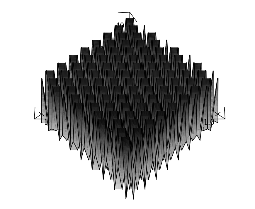
Figure 1: Plot of $10+50\sin(\frac{2\pi x}{0.125}+\frac{2\pi y}{0.125})$.

The forcing function and thus the solution change with the mesh size.

$$\begin{array}[]{c|cccccc}{\small\varepsilon\Downarrow\setminus h\Rightarrow}&{\small 0.125}&{\small 6.2E-2}&{\small 3.1E-2}&\text{ }{\small 1.6E-2}&{\small 7.8E-3}&{\small 3.9E-3}\\ \hline\cr{\small 1}&{\small 1.1E2}&{\small 1.0E2}&{\small 1.0E2}&{\small 1.0E2}&{\small 1.0E2}&{\small 1.0E2}\\ {\small 6.3E-2}&{\small 5.6E2}&{\small 5.6E2}&{\small 5.6E2}&{\small 5.6E2}&{\small 5.6E2}&{\small 5.6E2}\\ {\small 3.9E-3}&{\small 7.4E3}&{\small 7.5E3}&{\small 7.6E3}&{\small 7.6E3}&{\small 7.7E3}&{\small 7.7E3}\\ {\small 2.4E-4}&{\small 1.1E5}&{\small 1.1E5}&{\small 1.2E5}&{\small 1.2E5}&{\small 1.2E5}&{\small 1.2E5}\\ {\small 1.5E-5}&{\small 1.8E6}&{\small 1.8E6}&{\small 1.8E6}&{\small 1.8E6}&{\small 1.8E6}&{\small 1.9E6}\\ {\small 9.5E-7}&{\small 2.9E7}&{\small 2.9E7}&{\small 2.9E7}&{\small 2.9E7}&{\small 2.9E7}&{\small 2.9E7}\\ {\small 6.0E-8}&{\small 4.7E8}&{\small 4.6E8}&{\small 4.6E8}&{\small 4.6E8}&{\small 4.6E8}&{\small 4.6E8}\end{array}$$

$$\text{Table 3: Values of }Est.2\simeq\frac{||f^{h}||}{||u^{\varepsilon}||}\text{, P1 elements}$$

For comparison with the last row in Table 3, the values of $Est.1\simeq h^{-2}+\varepsilon^{-1}h^{-2}$ for $\varepsilon=6.0E-8$ are

$$\begin{array}[]{cccccc}{\small 1.1E9}&{\small 4.3E9}&{\small 1.7E10}&{\small 6.9E10}&{\small 2.7E11}&{\small 1.1E12}\end{array}.$$

In Table 3, as $\varepsilon\downarrow 0,$ $Est.2$ grows roughly like $\varepsilon^{-1}$. The stable behavior of $Est.2$ as $h\downarrow 0$ is unexpected. The behavior of $Est.3\simeq\varepsilon^{-1}h^{-1}\frac{||\nabla\cdot u^{\varepsilon}||}{||u^{\varepsilon}||}$ for P1 elements was similar, so not presented.

We now present tests of P2 elements for this problem. In this test $Est.3$ was larger than $Est.2,$ so we present only $Est.3$ data.

$$\begin{array}[]{c|cccccc}{\small\varepsilon\Downarrow\setminus h\Rightarrow}&{\small 0.125}&{\small 6.2E-2}&{\small 3.1E-2}&\text{ }{\small 1.6E-2}&{\small 7.8E-3}&{\small 3.9E-3}\\ \hline\cr{\small 1}&{\small 25}&{\small 49}&{\small 1.0E2}&{\small 2.0E2}&{\small 4.0E2}&{\small 7.9E2}\\ {\small 6.3E-2}&{\small 3.8E2}&{\small 7.5E2}&{\small 1.5E3}&{\small 3.0E3}&{\small 6.0E3}&{\small 1.2E4}\\ {\small 3.9E-3}&{\small 6.0E3}&{\small 1.2E4}&{\small 2.4E4}&{\small 4.8E4}&{\small 9.6E4}&{\small 1.9E5}\\ {\small 2.4E-4}&{\small 9.6E4}&{\small 1.9E5}&{\small 3.8E5}&{\small 7.7E5}&{\small 1.5E6}&{\small 3.1E6}\\ {\small 1.5E-5}&{\small 1.5E6}&{\small 3.1E6}&{\small 6.2E6}&{\small 1.2E7}&{\small 2.5E7}&{\small 4.9E7}\\ {\small 9.5E-7}&{\small 2.5E7}&{\small 4.9E7}&{\small 9.8E7}&{\small 2.0E8}&{\small 3.9E8}&{\small 7.9E8}\\ {\small 6.0E-8}&{\small 3.9E8}&{\small 7.9E8}&{\small 1.6E9}&{\small 3.2E9}&{\small 6.3E9}&{\small 1.3E10}\end{array}$$

$$\text{Table 4: Values of }Est.3\simeq\varepsilon^{-1}h^{-1}\frac{||\nabla\cdot u^{\varepsilon}||}{||u^{\varepsilon}||}\text{ },\text{ P2 elements}$$

For comparison with the last row in Table 4, $Est.1$ values for $\varepsilon=6.0E-8$ are

$$\begin{array}[]{cccccc}{\small 1.1E9}&{\small 4.3E9}&{\small 1.7E10}&{\small 6.9E10}&{\small 2.7E11}&{\small 1.1E12}\end{array}.$$

For this problem, down the columns (fixed $h$, $\varepsilon\downarrow 0$ ) the computed estimate of $\kappa(u^{\varepsilon})$ grows roughly like $\varepsilon^{-1}$. Reading across the columns, the values in each row grow like $h^{-1}$ (not $h^{-2}$). In all cases, $Est.3$ was smaller than $Est.1$.

4 Conclusions

The classical view is that two significant issues are impediments to penalty methods giving low cost and highly accurate velocity approximates. The first is ill-conditioning of the resulting system matrix. We have shown that the effective condition number $\kappa(u^{\varepsilon})$ is much smaller than the usual condition number due to the magnitude of the components in the penalized eigenspaces being small in a precise sense. Motivated by this theoretical result, we then compared the derived estimates of ill-conditioning on two test problems and for two elements. With P1 elements, ill-conditioning was not as severe as $\mathcal{O}(\varepsilon^{-1}h^{-2})$ but followed $\varepsilon^{-1}$ growth as $\varepsilon\rightarrow 0$. For P2 elements and approximating a smooth solution, $\kappa(u^{\varepsilon})$ was smaller the expected $\kappa\sim h^{-2}$ for the discrete Laplacian. With both P1 and P2 elements, and an academic test problem with data oscillating as fast as the mesh allows, ill-conditioning was not as severe as the expected $\mathcal{O}(\varepsilon^{-1}h^{-2})$ but also followed the $\varepsilon^{-1}$ pattern as $\varepsilon\rightarrow 0$.

The second significant issue is the difficulty in the selection of an effective value of $\varepsilon$. While the most commonly recommended, e.g. [8, 14], choices are $\varepsilon=$ time step, mesh width, and (machine epsilon)^1/2, none have proven reliably effective. Recent work of [17, 25] may resolve this impediment by an algorithmic, self-adaptive selection of $\varepsilon$ based on some indicator of violation of incompressibility. The estimates in Theorem 2.1 give insight into the resulting conditioning when this is done. Let $TOL$ denote a specified tolerance. If $\varepsilon$ is adapted so that the penalized solution $u^{\varepsilon}$ satisfies $\frac{||\nabla\cdot u^{\varepsilon}||}{||u^{\varepsilon}||}\leq TOL,$ then, Theorem 2.1 immediately implies $\kappa(u^{\varepsilon})$ satisfies

(2) $$\kappa(u^{\varepsilon})\leq Ch^{-2}\left(1+h\frac{TOL}{\varepsilon}\right).$$

If $\varepsilon$ is adapted so that the penalized solution $u^{\varepsilon}$ satisfies $\frac{||\nabla\cdot u^{\varepsilon}||}{||\nabla u^{\varepsilon}||}\leq TOL,$ then, similarly, Theorem 2.1 implies $\kappa(u^{\varepsilon})$ satisfies

(3) $$\kappa(u^{\varepsilon})\leq Ch^{-2}\left(1+\frac{TOL}{\varepsilon}\right).$$

For (3), rewrite $||\nabla\cdot u^{\varepsilon}||/||u^{\varepsilon}||$ as $\left(||\nabla\cdot u^{\varepsilon}||/||\nabla u^{\varepsilon}||\right)\left(||\nabla u^{\varepsilon}||/||u^{\varepsilon}||\right)$. The inverse estimate, A1, implies $||\nabla u^{\varepsilon}||/||u^{\varepsilon}||\leq Ch^{-1}$, yielding (3).

The numerical tests suggest that two factors not considered in Theorem 2.1 are significant. The first is whether the finite element space has a nontrivial, divergence-free subspace. The second is the influence of smoothness of the sought solution or its problem data on effective conditioning. In addition, highly refined meshes are used in practical flow simulations and the linear system often has large skew symmetric part. The extension of the analysis herein to include these effects is an open problem.

References

- [1] A.O.H. Axelsson, Condition Numbers for the Study of the Rate of Convergence of the Conjugate gradient Method, p. 3-33 in: Proc. of the 2nd IMACS Internat. Symposium on Iterative Methods in Linear Algebra, Blagoevgrad, Bulgaria, June 17-20, 1995.
- [2] A.O.H. Axelsson, Iterative solution methods, Cambridge University Press, 1996..
- [3] A.O.H. Axelsson and I.E. Kaporin, On the sublinear and superlinear rate of convergence of conjugate gradient methods. Numerical Algorithms, 25 (2000) 1-22.
- [4] A.O.H. Axelsson and I.E. Kaporin, Error norm estimation and stopping criteria in preconditioned conjugate gradient iterations. Numerical Linear Algebra with Applications, 8 (2001) 265–286.
- [5] J.M. Banoczi, Nan-Chieh Chiu, Grace E. Cho and I.C.F. Ipsen, The lack of influence of right-hand side on accuracy of linear system solution, SIAM Journal on Scientific Computing, 20 (1998) 203–227.
- [6] S.C. Brenner, and L.R. Scott, The mathematical theory of finite element methods, New York: Springer, 2008.
- [7] C. Brezinski, Error estimates for the solution of linear systems, SIAM Journal on Scientific Computing, 21 (1999) 764–781.
- [8] G.F. Carey and R. Krishnan, Penalty approximation of Stokes flow, Comp. Meth. Appl. Mech. Eng., 35 (1982) 169–206.
- [9] T.F. Chan and D.E. Foulser, Effectively well-conditioned linear systems. SIAM Journal on Scientific and Statistical Computing, 9 (1988) 963–969.
- [10] P. G. Ciarlet, The finite element method for elliptic problems, vol. 40 of Classics in Applied Mathematics. Society for Industrial and Applied Mathematics (SIAM), Philadelphia, PA, 2002. (Reprint of the 1978 original).
- [11] S. Christiansen and P.C. Hansen, The effective condition number applied to error analysis of certain boundary collocation methods, Journal of Computational and Applied Mathematics, 54(1994) 15–36.
- [12] S.G. Demko, Condition numbers of rectangular systems and bounds for generalized inverses, Linear Algebra and its Applications, 78 (1986) 199-206.
- [13] Qiang Du, Desheng Wang and Liyong Zhu, On Mesh Geometry and Stiffness Matrix Conditioning for General Finite Element Spaces, SIAM Journal on Numerical Analysis, 47 (2009) 1421-1444.
- [14] J.C. Heinrich and C.A. Vionnet, The penalty method for the Navier-Stokes equations. Archives of Computational Methods in Engineering, 2 (1995) 51-65.
- [15] V. John, A. Linke, C. Merdon, M. Neilan, and L.G. Rebholz, On the divergence constraint in mixed finite element methods for incompressible flows. SIAM Review, 59 (2017), 492-544.
- [16] I.E. Kaporin, New convergence results and preconditioning strategies for the conjugate gradient method. Numerical Linear Algebra with Applications, 2 (1994) 179-210.
- [17] K. Kean, Xihui Xie and Shuxian Xu, A Doubly Adaptive Penalty Method for the Navier Stokes Equation, preprint, 2021, https://arxiv.org/abs/2201.03978.
- [18] Z.C. Li and H.T. Huang, Effective condition number for numerical partial differential equations. Numerical Linear Algebra with Applications, 7 (2008) 575-94.
- [19] Z.C. Li, H.T. Huang and J. Huang, Superconvergence and stability for boundary penalty techniques of finite difference methods. Numerical Methods for Partial Differential Equations, 24 (2008) 972-90.
- [20] J. von Neumann and H.H. Goldstine, Numerical inverting of matrices of high order, Bulletin of the American Mathematical Society, 53 (1947) 1021-1099.
- [21] J.R. Pragua, New condition number for matrices and linear systems, Computing 41 (1989) 211–213.
- [22] T. Tao and V. Vu, Smooth analysis of the condition number and the least singular value, Mathematics of Computation, 79 (2010) 2333-2352.
- [23] A.M. Turing, Rounding-off errors in matrix processes, Quarterly Journal of Mechanics and Applied Mathematics, 1 (1948): 287-308.
- [24] J.H. Wilkinson, Rounding Errors in Algebraic Processes, Volume 32 of National Physical Laboratory Notes on Applied Science, (HMSO), London, 1963.
- [25] Xihui Xie, On Adaptive Grad-Div Parameter Selection, technical report, https://doi.org/10.48550/arXiv.2108.01766, 2021.