FETILDA: An Effective Framework For Fin-tuned Embeddings For Long Financial Text Documents

Abstract

Unstructured data, especially text, continues to grow rapidly in various domains. In particular, in the financial sphere, there is a wealth of accumulated unstructured financial data, such as the textual disclosure documents that companies submit on a regular basis to regulatory agencies, such as the Securities and Exchange Commission (SEC). These documents are typically very long and tend to contain valuable soft information about a company’s performance, which is usually not captured in predictive analyses that only utilize quantitative data. It is therefore of great interest to learn predictive models from these long textual documents, especially for forecasting numerical key performance indicators (KPIs). Whereas there has been a great progress in natural language processing via pre-trained language models (LMs) learned from tremendously large corpora of textual data, they still struggle in terms of effective representations for long documents. Our work fills this critical need, namely how to develop better models to extract useful information from long textual documents and learn effective features that can leverage the soft financial and risk information for text regression (prediction) tasks. In this paper, we propose and implement a deep learning framework that splits long documents into chunks and utilizes pre-trained LMs to process and aggregate the chunks into vector representations, followed by attention-based sequence modeling to extract valuable document-level features. We evaluate our model on a collection of 10-K public disclosure reports submitted annually by US banks, and another dataset of reports submitted by US companies. Overall, our framework outperforms strong baseline methods for textual modeling as well as a baseline regression model using only numerical data. Our work provides better insights into how utilizing pre-trained domain-specific and fine-tuned long-input LMs in representing long documents can improve the quality of representation of textual data, and therefore, help in improving predictive analyses.

Keywords machine learning $\cdot$ information extraction $\cdot$ natural language processing $\cdot$ text regression $\cdot$ language models $\cdot$ long text documents $\cdot$ financial documents $\cdot$ 10-K reports $\cdot$ SEC disclosure documents

1 Introduction

Unstructured data such as text is growing very fast in different domains. Especially, textual data from financial documents has been found to be beneficial in making predictions [1]. Utilizing such large volumes of textual data requires natural language processing (NLP) and machine learning (ML) techniques. These techniques summarize the text as (a set of) numeric feature vectors, which are called representations or embeddings, and which can in turn serve as inputs to machine learning models to predict some target variables.

The traditional approach for text-based learning is via the Term Frequency - Inverse Document Frequency (TF-IDF) method [2], which can represent the document as a long numeric vector of TF-IDF scores for each word. However, TF-IDF does not attempt to directly extract the latent semantic information within the text. The current progress in text representations was initiated by word embedding methods, such as word2vec [3] and GloVe [4], which capture both the lexical and semantic information of a document to some extent. The main idea is to learn word representations based on the context of each word. However, these methods learn only a single, static representation for each word, and do not take into consideration the phenomenon of polysemy, where a word can change its meaning depending on the context (for example, the the word ‘bank’ in the financial context has a very different meaning compared to the ‘bank’ of a river). The state-of-the-art (SOTA) pre-trained language models, such as GPT [5] and BERT [6] are built on top of the very effective Transformer-based attention model [7], which can learn contextual word embeddings. These embeddings are dynamic in terms of the surrounding block or context of the word, so that the same word can get different representations that are most effective in capturing the lexical and semantic information. These models have shown SOTA performance on a variety of downstream tasks such as question answering, text classification, and regression.

While much progress has been made in NLP, our focus in this paper is on the relatively under-examined area of financial text documents. Specifically, we are focusing on the 10-K financial reports that companies in the US submit annually to the Securities and Exchange Commission (SEC). These reports describe a company’s activities, progress, and risks in the interest of the company’s stakeholders. The detailed content of these reports is helpful in evaluating the status of the company as well as predicting future metrics from forward-looking statements. One of the key parts of 10-K reports is Item 7, namely, the Management’s Discussion and Analysis (MDA) section. Another key part is Iten 1A, namely, the Risk Factors section. Textual data contained in these 10-K reports are predictive of the volatilities that companies have in the stock market, and can be helpful in predicting failures of financial institutions, as well [1, 8]. But, in these approaches, they use an expert-generated sentiment dictionary by Loughran and McDonald (L&M) [9] to generate the vector of features. For example, Kogan et al. [10] utilized the MDA section to predict the return volatility of stocks using the L&M word list. In addition, the L&M word list was expanded using word2vec [3]. Then, it was used in Tsai and Wang [11].

As mentioned above, moving beyond the static embedding methods, it is important that we take into consideration the contextual information of words, since specific words can have different meanings in the financial context than those in the general context, the nuances of which may not be apparent to laypersons. For this, we can utilize the recent contextual language models to represent long documents, such as the 10-K reports, in order to construct effective models for conducting predictive analyses. However, extracting “good” representations for such long documents remains a challenging task: the length of the 10-K documents poses both a methodological and ontological burden. Methodologically, financial reports are significantly longer, compared to the maximum length of a textual sequence that BERT [6]-based models can handle. For instance, the Management Discussion and Analysis (MD&A) section of the 10-K reports that companies publish annually is usually around 12,000 word-tokens. BERT-based models have a restriction on the maximum number of tokens, around 512, with some newer models, such as Longformer [12] and BigBird [13], reaching up to 4,096 tokens. Ontologically, the challenge is the classic machine learning task of extracting or learning informative features that can represent the input well. This question becomes quite complex in the context of representing a long document. Contextual word embeddings are well suited for this given their ability to “understand” different meanings for a word in different contexts. However, it remains an open question as to how to combine the various contextual word embeddings into an effective document level embedding.

An additional challenge is that the SOTA language models are pre-trained on massive and generic corpuses, e.g., from web crawls, wiki media, and so on. However, to be effective for the financial context, it is important for LMs to learn domain-adapted and task-specific representations of long documents in order to meaningfully support predictive analyses. This can usually be achieved either by pre-training (from scratch) a domain-specific language model on a huge financial corpus to adapt to its particular domain, or by fine-tuning a pre-trained LM on a specific financial dataset for the downstream tasks, or by combining the two approaches of adapting the LM to a particular financial domain followed by fine-tuning on downstream tasks. Recently there have been several attempts at pre-training BERT on large financial corpuses to adapt it for tasks in the financial domain. Liu et al.[14], Yang et al. [15], Araci [16], and DeSola et al.[17], each pre-trained the BERT model from scratch on financial corpora, such as financial news, corporate reports, financial websites, and so on. Incidentally, all four approaches are called FinBERT!

To address the long document representation challenge within the context of financial disclosure documents, we propose a novel framework called Fin-tuned Embeddings of Texts In Long Document Analysis (FETILDA). Our approach is particularly designed for downstream predictive or regression tasks, where the input document representations are combined with other numeric attributes (if available) to predict a target response variable of interest, such as key performance indicators (e.g., return on assets, earnings per share), stock volatility, and so on. FETILDA comprises a novel chunk-based deep learning framework, where a long document is split into several smaller chunks and then each chunk is processed using an appropriate language model (e.g., BERT [6], FinBERT [15] or Longformer [12]). The layers of the LM can remain frozen, or they may be unfrozen for fine-tuning, or only the last layer can be frozen. The chunk level representations are then pooled together using a Bi-LSTM model equipped with self-attention mechanism. The pooled chunks are then aggregated into a document level representation, which serves as input for a fully connected linear neural network for target variable prediction. We can also use the document representations as inputs to Support Vector and Kernel regression models. We evaluate our framework using two different corpuses: i) 10-K reports submitted annually to the SEC by US banks for the period from 2006 to 2016, ii) 10-K reports for all US companies from 1996 to 2013 [18]. We have conducted extensive experiments using these datasets and applied our framework to different predictive analysis regression tasks: i) predictive metrics of a bank’s financial performance, such as Return on Assets (ROA), Earnings Per Share (EPS), Return on Equity (ROE), Tobin’s Q Ratio (TQR), Leverage Ratio (LR), Tier 1 Capital Ratio (T1CR), Z-Score (Z) and Market to Book Ratio (MBR); ii) analysis of a company’s stock market volatility. Our results compared against the different baseline methods show that FETILDA performs significantly better and yields SOTA results for long financial text regression tasks. In summary, our main contributions are:

• We propose a SOTA deep learning framework for long document regression tasks in the financial domain. Our FETILDA approach is designed to learn effective document level representations via a sequential chunking approach combined with an attention mechanism. As such our approach combines the best of both the attention-based Transformer model and Bi-LSTM recurrent networks.

• We conduct an extensive set of experiments to quantitatively showcase the effectiveness of our FETILDA approach. We applied the model on two different 10-K datasets, and on 9 different regression tasks. We show that FETILDA outperforms several different baseline methods, and achieves state-of-the-art results on long financial documents.

2 Related Work

Machine learning plays an important role in financial analytics. One of the important areas of finance is investment stock return forecasting, as well as fundamentals forecasting and risk modeling, that mainly employ quantitative or numeric data [19]. Different ML models such as Support Vector Machines (SVMs), single hidden layer Feed-forward Neural Networks and Multi-layer Perceptrons (MLPs) were used for the prediction of future price movements in [20]. They mainly used two sets of features for their ML classifiers: (1) handcrafted features formed on the raw order book data and (2) features extracted using ML algorithms. Some other models such as Random Forest [21], XGBoost [22], Bidirectional Long Short-Term Memory (Bi-LSTM) and stacked LSTMs [23] were also implemented to predict business risk and stock volatility. The main limitation of these works is that they ignore valuable textual data that can provide more insight into the intangible features such as sentiment, knowledge capital, risk culture, and so on.

2.1 Textual Data: Sentiment Analysis

An approach to predict financial quantitative variables is using financial textual sources such as news reports, analyst assessments, earnings call transcripts, and company filing reports. In [24], textual features were created by using the negative words in the Harvard-IV-4 TagNeg dictionary and constructing a document-term matrix from the news stories. These features were used to predict firms’ earnings and stock returns. A novel tree-structured LSTM was proposed to automatically measure the usefulness of financial news using both text and cumulative abnormal returns [25]. A dual-layer attention-based neural network model was developed to predict stock price movement using the text in financial news [26]. Estimating the value of text in financial news is important because it drives the investment decision making process.

Financial sentiment analysis is challenging because of lack of labeled data specific to this domain. Moreover, the general-purpose pre-trained language models fail to capture the financial context. [16] proposed the FinBERT model, which can be fine-tuned on the financial sentiment analysis dataset (FiQA) to outperform the general BERT model. Besides financial news, in [10], the authors constructed textual features from 10-K reports. They used these features to predict the future stock volatility indicating the effectiveness of text. A deep learning model trained on the SEC filings was used to improve the prediction of company’s stock price over the traditional ML models [27].

The authors in [28] and [11] extracted additional textual features by expanding the L&M sentiment word list [9] semantically and syntactically, using word2vec [3]. Similarly, the uncertainty word list in L&M dictionary was expanded using word2vec to predict stock volatility [29]. The authors in [30] expanded the L&M dictionary by training industry-specific word embedding models using word2vec to predict volatility, analyst forecast error and analyst dispersion. [31] showed how automatic domain adaption of the L&M sentiment list using word2vec [3] improved the prediction of excess return and volatility. The aforementioned dictionary expansion approaches used word2vec model to select the top $k$ closest words to the words existing in the L&M dictionary. Since word2vec is a model based on static word embeddings, it fails to capture the dynamic context of the words.

2.2 Language Models in Finance

In terms of domain-adapted pre-trained LMs, in the English-speaking Finance sphere, four models have been proposed and implemented, all named FinBERT: Liu et al. [14], Yang et al. [15], Araci [16], and DeSola et al. [17], all of which are pre-trained to adapt to different financial domains. Originally, in the general domain, BERT [6] was pre-trained on two corpora: BooksCorpus (0.8 billion words), and English Wikipedia (2.5 billion words), forming a total of 3.3 billion words, so the idea of these financial language models is to take the original model, and pre-train it on their respective financial corpora.

Araci [16] was the first to propose FinBERT as a pre-trained domain-adapted BERT [6] on a corpus called TRC2-financial, which includes 46,143 documents with more than 29M words and nearly 400K sentences, from a set of Reuters news stories. In experimentation, they saw a 15% increase in accuracy for classification tasks, a significant margin. Liu et al. [14] focused on financial news and dialogues present on websites, and collected three financial corpora: 13 million financial news (15GB) and financial articles (9GB) from Financial Web, totaling 24GB and 6.38 billion words; financial articles from Yahoo! Finance, totaling 19GB and 4.71 billion words; and question-answer pairs about financial issues from Reddit, totaling 5GB and 1.62 billion words. They pre-trained their model on these corpora to adapt it to the financial news and dialogues domain. In experimentation, they saw their model outperform BERT [6] on all the financial tasks in their experiments, in terms of accuracy, precision, and recall [14]. Yang et al. [15] focused on financial and business communications that companies produce, and collected a corpus of three types of data: 10-K and 10-Q reports, totaling 2.5 billion word tokens; earnings call transcripts, totaling 1.3 billion word tokens; and analyst reports, totaling 1.1 billion word tokens [15]. They report that their model outperforms BERT [6] in three sentiment analysis tasks, all by significant margins [15]. DeSola et al. [17] introduced another domain-specific pre-trained language model, also named FinBERT, for financial NLP applications. This model was trained on the 10-K filings from 1998 to 1999 and from 2017 to 2019, totaling 497 million words, and it showed better performance than BERT on the masked LM and next sequence prediction tasks.

2.3 Long Document Language Models

Apart from LMs adapted to specialized domains, there has been a slew of papers on state-of-the-art pre-trained LMs in the general domain, such as GPT-1 [5], GPT-2 [32], GPT-3 [33], T-5 [34], ELECTRA [35], and so on. These are massive models trained on enormous corpora, but the challenge of representing long documents persists, in that these models still cannot handle long textual sequences, due to the quadratic computational complexity that they usually entail.

To tackle this challenge head-on, several recent works, such as Longformer [12], ETC [36], and BigBird [13], have been proposed, all of which innovate on the self-attention mechanism in order to reduce the computational complexity from quadratic to linear, which then enables it to process longer sequences of text. In addition, more recent works on transformer models with linear attention, such as Reformer [37] and Nystromformer [38], innovate on how to mathematically approximate the self-attention matrix calculations with less time and space complexity, instead of changing the self-attention mechanism.

Longformer [12] replaces the full self-attention matrix, which scales quadratically with the length of the input sequence, with three types of sparse attention schemes: sliding window attention, which selects only the entries on the descending diagonal line of the self-attention matrix, with the ‘thickness’ of the line being a certain size; dilated window attention, which adds gaps of a certain size in between the sliding window, making the descending diagonal line dilated; global attention, which has certain specific tokens attend to all the tokens across the sequence, both horizontally and vertically, thereby enabling global contextual representation of the sequence. Longformer was shown to outperform baseline methods consistently, and particularly, its results were more apparent where the experiment required long contextual information.

Extended Transformer Construction (ETC) [36] is very similar to Longformer, with nuanced variations. ETC replaces the full self-attention matrix with global-local attention, which splits the self-attention matrix into four parts: global-to-global, which is a small square on the top left of the matrix, where certain special global tokens attend to each other; global-to-long, which is a horizontal rectangle on the top right of the matrix, where global tokens attend to regular tokens; long-to-global, which is a vertical rectangle on the bottom left of the matrix, where regular tokens attend to global tokens; long-to-long, which is a compressed version of the descending diagonal line in the large square on the bottom right of the matrix, essentially a sliding window attention compressed into a rectangular matrix, where regular tokens attend to other regular tokens in its window. In experimentation, ETC yielded state-of-the-art results, especially in question answering scenarios.

BigBird [13] extends further on ETC [36], adding random sparse attention into the mix, building on top of the global-local attention mechanism of ETC. Random entries in the self-attention matrix are selected to generalize over the full matrix. From a graph theory perspective, this means a shorter average path between any two nodes, making it a better approximation of the full graph. And from a NLP perspective, in most texts, there tends to be locality of reference, where a word relates closely with words around it, so BigBird tries to account for this with their particular random sparse attention scheme.

2.4 Chunking-based Representation Schemes

Similar to the FETILDA approach we propose in this paper, other approaches to constructing document-level representations have been proposed in other works. Yang et al. [39] proposed a method similar to ours in their hierarchical approach of using sentence blocks to construct document representations, for the purpose of document matching. In their approach, the sentence block representations are passed through a transformer model and the first token of the resulting output is used as the document representation. They also have an option to concatenate the sentence representations via attention based weights. With this framework, they are able to handle maximum document lengths ranging from 512 to 2,048 word tokens. However, in our use case, FETILDA has to deal with with much longer documents than 2,048 word tokens. Even just one section of the 10-K reports that we learn on, namely, Item 7, averages around 12,000 words, and can be more than 24,000 tokens after tokenization. Therefore, instead of sentence-level blocks, we use (paragraph-level) chunks, and we weigh these chunks using their respective attention scores obtained by a self-attention mechanism. Finally, we pool the weighted chunks together into a document representation, using a bi-LSTM network. In our experiments, we utilize different models that can enable us to have the maximum chunk length range from 512 up to 8,192 word tokens, which then enables us to generate representations for documents that average 24,000 word tokens. Furthermore, while both our approach and their approach focus on obtaining a good document representation, the final goals are different: we aim to learn financial text features predictive of future target metrics of banks and companies, while their aim is document matching.

Gong et al. [40] proposed a recurrent chunking mechanism for the purpose of machine reading comprehension, where the machine is given a long document and a question, and is required to extract a piece of text from the document as the answer to the questions. Towards that end, they needed the chunking mechanism to be such that the separation point of various chunks would not cut the correct answer in half, nor prevent surrounding contexts from being retained. Therefore, their main innovation is in enabling a more flexible chunking policy, and in a recurrent chunking mechanism that can provide context surrounding a chunk segment. In experimentation, they use BERT, which enables maximum sequence lengths ranging from 192 to 512 word tokens. Our framework takes a different approach to the chunking policy, since our goal is the extraction of predictive financial text features from the document. Moreover, we also try to increase the maximum sequence length of a chunk up to 8,192 word tokens, which then allows us to take in more information in one chunk in an organic way.

In more recent work, Grail et al. [41] use a bi-GRU network to pool the chunks together, instead of a bi-LSTM network. But the purpose of their framework is long document summarization, instead of extracting predictive text features. In their approach, they use BERT as the LM, and therefore, can only process up to 512 word tokens for a chunk. Further, they consider their approach to be an alternative to long sequence LMs such as Longformer. Instead of considering long sequence LMs as alternatives, we incorporated them into our FETILDA framework. Therefore, in our approach, we experiment with various underlying LMs for FETILDA, be it BERT-based models, or long sequence LMs, or linear attention transformer LMs, enabling us to have different maximum sequence lengths ranging from 512 to 8,192 tokens.

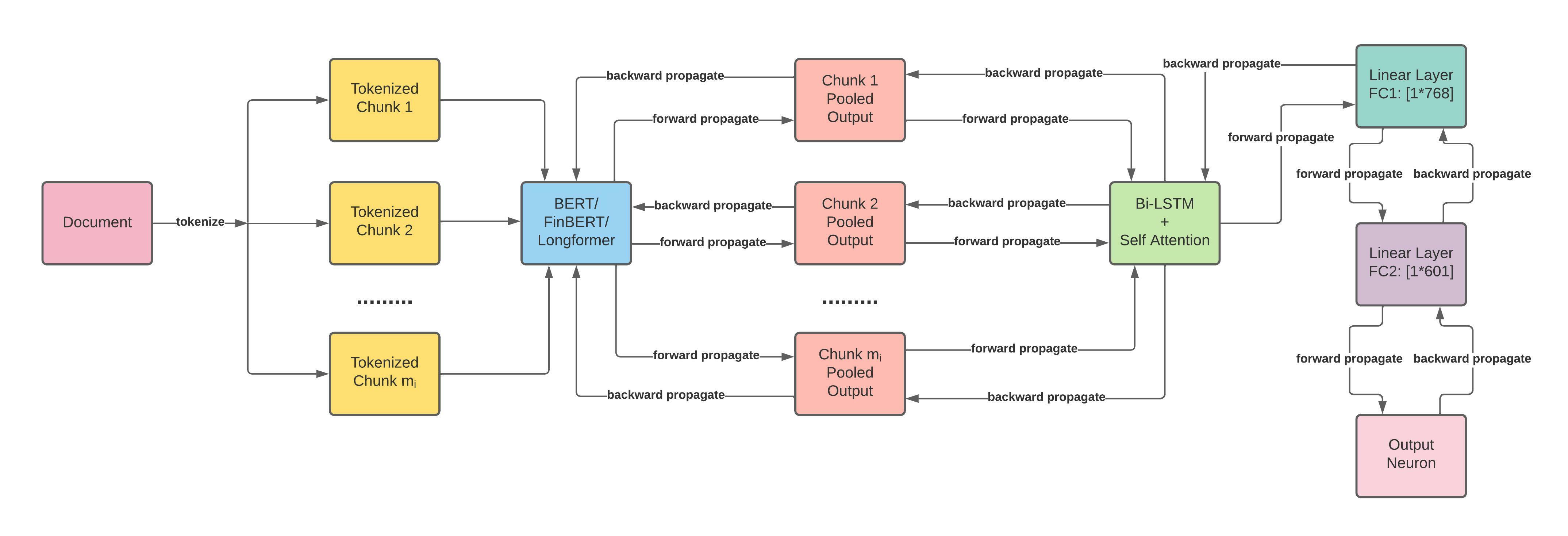
Figure 1: FETILDA: Overall Framework.

3 FETILDA: Long Document Representation

Figure 1 shows the complete FETILDA framework. FETILDA first splits a long document into smaller fragments or chunks, then processes each chunk using a language model, all of whose layers are fully unfrozen for fine-tuning, then pools the chunks together using a Bi-LSTM layer endowed with a self-attention mechanism into an aggregate vector representation of the entire document. The chunk representations are extracted from the underlying language model (BERT [6], FinBERT [15], Longformer [12], or Nystromformer [38]) using several different pooling strategies including using the default pooler output and combining the features from the last few layers. These chunk sequences are passed onto a Bi-LSTM model whose hidden context states and outputs are used to learn chunk-level attention scores to extract the final document embedding. Finally, the document embedding is passed through the linear layers to obtain the final target prediction. In addition, we perform task-specific fine-tuning on our entire model, including BERT, FinBERT, or Longformer, whose layers are fully unfrozen (or can be kept frozen if only pre-trained inputs are to be used), using MSE as the loss function. Overall, as shown in Figure 1, our methodology consists of four stages: (1) Chunk Generation, (2) Chunk-Level LM Pooling, (3) Document-Level Attention Pooling, and (4) Model Training and Fine-Tuning. We shall describe each of these next.

3.1 Chunk Generation

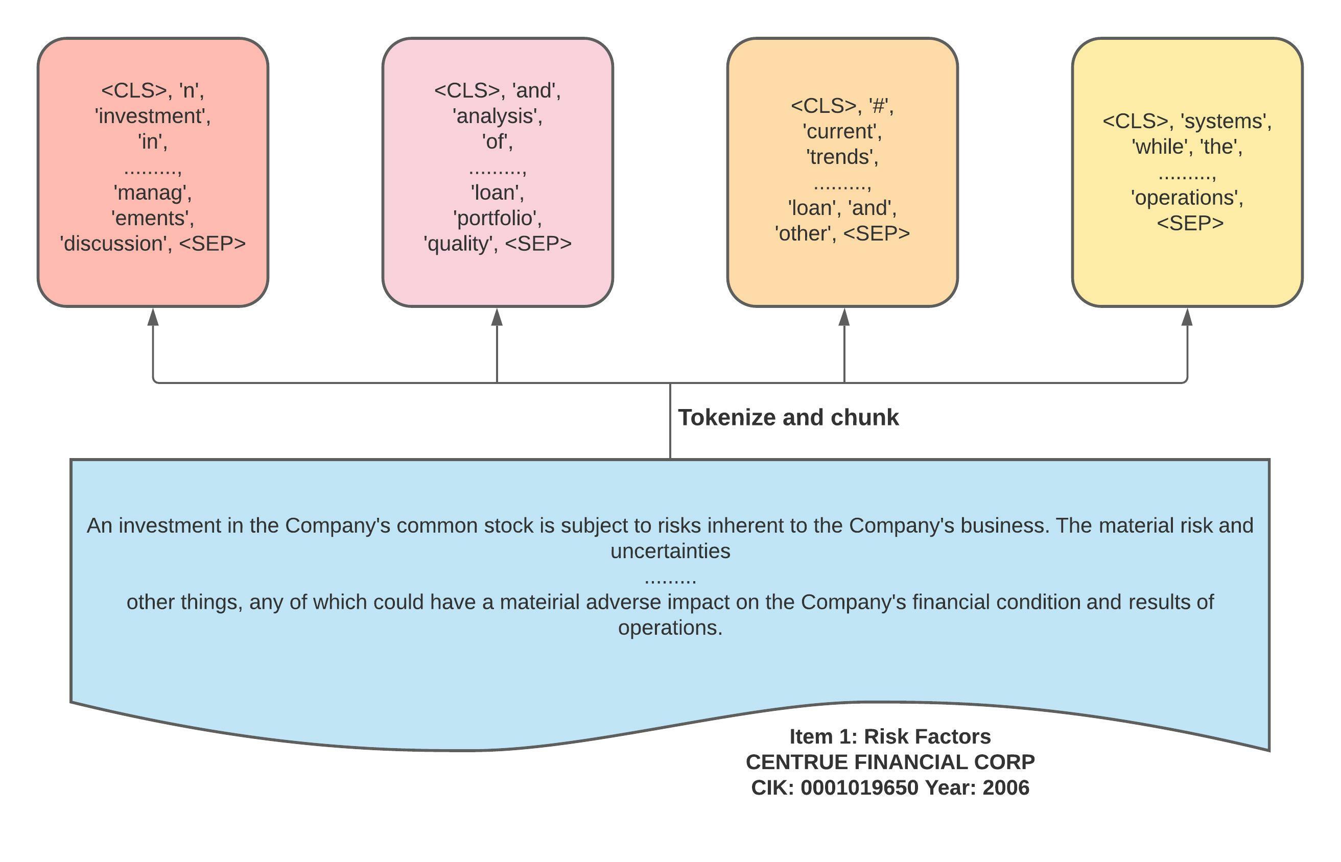
Figure 2: Chunk Generation

Let $L=\{d_{1},d_{2},\cdots,d_{N}\}$ denote a text corpus containing $N$ long documents, where $d_{i}$ denotes the $i$-th document in the corpus. We tokenize each document $d_{i}$ into a sequence of tokens $\{t_{1},t_{2},\cdots,t_{n_{i}}\}$, where $n_{i}$ is the number of tokens for document $d_{i}$. The document token sequence is divided into chunks of length $b$, where $b$ is the block or chunk size. Thus, each document $d_{i}$ can be represented as a sequence of chunks $\{c_{1},c_{2},\cdots,c_{m_{i}}\}$, with $m_{i}$ chunks of length $b$. We also prepend and append <CLS> and <SEP> tokens to each chunk, respectively, resulting in chunks of size $b+2$. The chunk size dictates a maximum of $b+2$ tokens for each chunk $c_{i}=\{t_{0},t_{1},\cdots,t_{b},t_{b+1}\}$, with $t_{0}=\texttt{<CLS>}$ and $t_{b+1}=\texttt{<SEP>}$. We experiment with $b+2=512$, $b+2=4096$ and $b+2=8192$, depending on the underlying language model used. For document where the last chunk has $k<b$ tokens, we pad the last chunk by appending the padding token (<PAD>) $(b-k)$ times to keep the chunk length intact. For each chunk, we also create an attention mask with [0] for padding tokens and [1] for non-padding tokens, which helps in attending only to the valid tokens and not the <PAD> tokens. Figure 2 shows an excerpt from Item 1 from a company’s 10-K report, and the tokenization and chunking process with four resulting chunks.

3.2 Chunk-Level Language Model Pooling

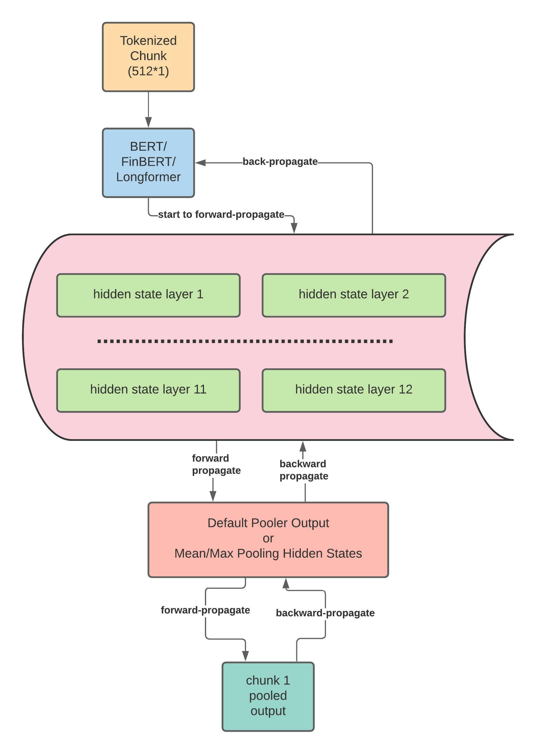
Figure 3: Chunk Level Language Model Pooling For Chunk Embeddings.

Given the sequence of chunks for a document, $\{c_{1},c_{2},\cdots,c_{m_{i}}\}$, we need to convert these into features vectors $\{\mathbf{c}_{1},\mathbf{c}_{2},\cdots,\mathbf{c}_{m_{i}}\}$, that represent the token sequence in each respective chunk as a whole. We use SOTA language models like BERT [6], Longformer [12], and FinBERT [15] to generate contextual token and chunk embeddings. We thus input each chunk into the underlying language model, which typically outputs 12 hidden state layers $\{l_{1},l_{2},\cdots,l_{12}\}$, where $l_{i}$ denotes layer $i$. The output of each of these layers contains $b+2$ hidden state vectors $\{\mathbf{z}_{0}^{l},\mathbf{z}_{1}^{l},\cdots,\mathbf{z}_{b+1}^{l}\}$, for $b+2$ tokens in the chunk, each of which has a size of 768, which is the dimensionality of the hidden states. The language model also yields a default pooler output, which is the embedding vector for the <CLS> token, the first token, of the last hidden state layer after processing and activation, denoted by $\mathbf{z}_{0}^{12}$. Figure 3 shows the schematic of how we use the underlying language model to generate the hidden state layers, as well as the default pooler output, which are then combined using various strategies outlined below to yield the chunk embedding vector $\mathbf{c}_{i}$ for each chunk $c_{i}$ within each document.

Creating contextual embeddings is challenging, since a word can have different meanings in different contexts. So it is important to first create contextual token embeddings and then experiment with different strategies to generate different chunk representations from these contextual embeddings. We therefore studied several approaches for creating the final chunk embedding vectors $\mathbf{c}_{i}$:

• Default pooler output: Since the <CLS> token embedding is an attention-weighted aggregation of all the tokens in a given chunk, each chunk $c_{i}$ can therefore be represented by the default pooling output vector $\mathbf{z}_{0}^{12}$ as the chunk embedding vector $\mathbf{c}_{i}$. The size of $\mathbf{c}_{i}$ is equal to the default hidden layer size of 768.

• Pooled hidden layers: The empirical evaluation conducted in BERT-as-a-Service [42] shows that using the last hidden layer gives the highest accuracy, but they also observed that it could also be more biased since it is the closest layer to the output layer. Hence, it is advisable to select the second-to-last hidden layer or a combination of different layers. In implementing this idea in practice, we take the set of all $b+2$ hidden state vectors from the penultimate layer, namely, $\{\mathbf{z}_{0}^{11},\mathbf{z}_{1}^{11},\cdots,\mathbf{z}_{b+1}^{11}\}$ and mean/max pool them into one vector of size 768, which, after some non-linear activation, can be used as the chunk embedding vector $\mathbf{c}_{i}$. In addition, we can also follow a similar approach by selecting the last four hidden layers, namely $\{\mathbf{z}_{0}^{9},\mathbf{z}_{1}^{9},\cdots,\mathbf{z}_{b+1}^{9}\}$, $\{\mathbf{z}_{0}^{10},\mathbf{z}_{1}^{10},\cdots,\mathbf{z}_{b+1}^{10}\}$, $\{\mathbf{z}_{0}^{11},\mathbf{z}_{1}^{11},\cdots,\mathbf{z}_{b+1}^{11}\}$, and $\{\mathbf{z}_{0}^{12},\mathbf{z}_{1}^{12},\cdots,\mathbf{z}_{b+1}^{12}\}$, and produce four mean/max pooled vectors in the same way. These four vectors and mean/max are pooled into one vector, which on activation can be used as the chunk embedding vector $\mathbf{c}_{i}$.

3.3 Document-Level Attention Pooling

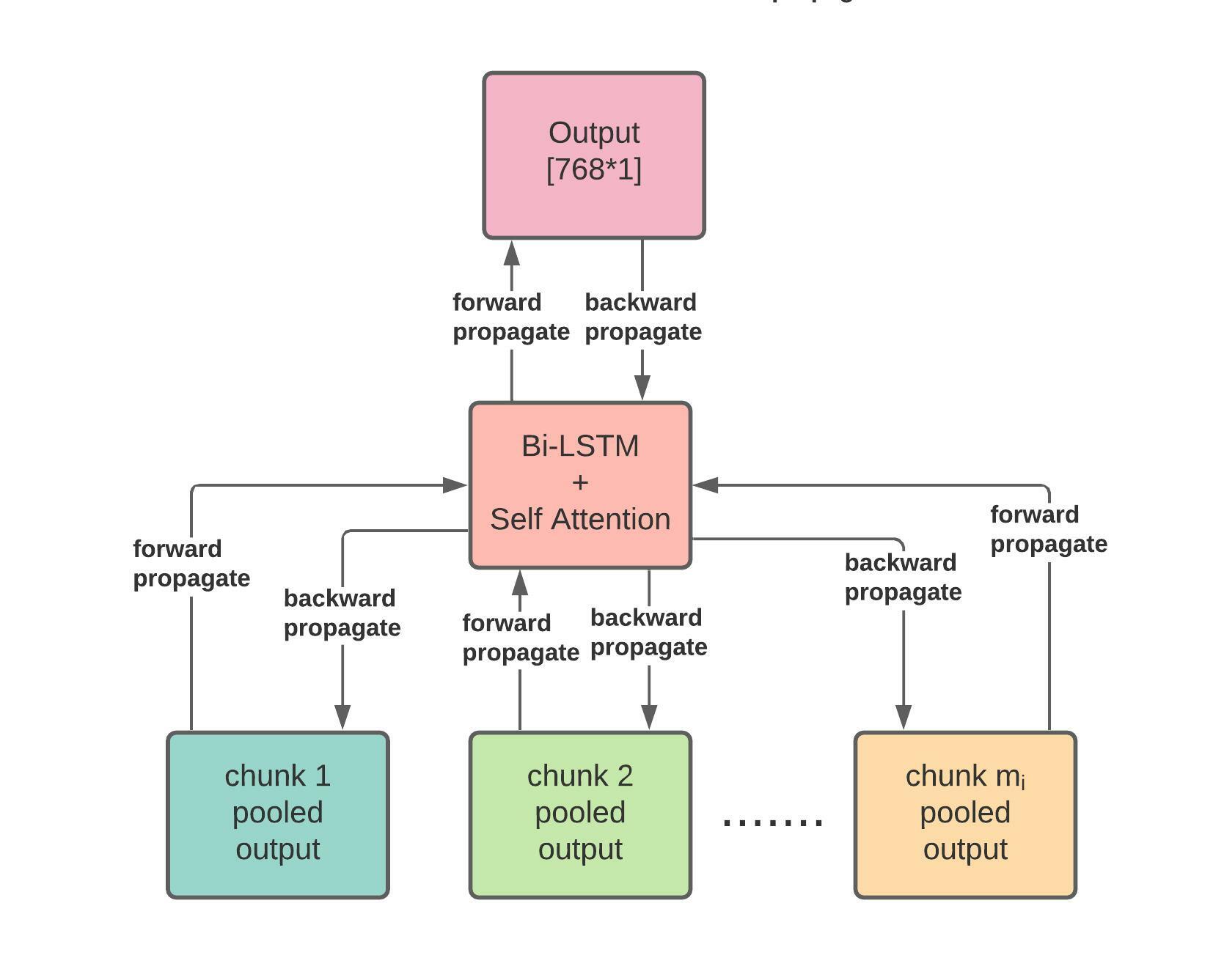
Figure 4: Attention Pooling via Bi-LSTM For Document Embeddings.

Given the chunk embedding vectors $\{\mathbf{c}_{1},\mathbf{c}_{2},\cdots,\mathbf{c}_{m_{i}}\}$, we need to aggregate them into an effective document vector $\mathbf{d}_{i}$ for document $d_{i}$. Since the chunks are sequential in nature, we can accomplish this using a recurrent Bi-LSTM model. However, not all chunks in a long document are equally important. It is crucial to score the chunks based on their importance in the document. For this, we introduce chunk-level attention within the Bi-LSTM model. Given a document, we input its chunk feature vectors $\{\mathbf{c}_{1},\mathbf{c}_{2},\cdots,\mathbf{c}_{m_{i}}\}$ into the Bi-LSTM model. The output and hidden state vectors of the Bi-LSTM for chunk $i$ are then obtained by concatenating the outputs and the hidden states in forward and backward pass, respectively. Formally,

$\mathbf{o}_{i}=\overrightarrow{\mathbf{o}_{i}}\oplus\overleftarrow{\mathbf{o}_{i}}\mathbf{h}_{i}=\overrightarrow{\mathbf{h}_{i}}\oplus\overleftarrow{\mathbf{h}_{i}}$ where $\oplus$ denotes concatenation, $\overrightarrow{}$ denotes forward and $\overleftarrow{}$ denotes backward models, and the $\mathbf{h}_{i}$ and $\mathbf{o}_{i}$ denote the hidden and output state vectors for chunk $c_{i}$, respectively ($i$ also denotes the $i$-th element of the chunk sequence). The attention score ${\alpha}_{i}$ for each chunk is calculated by taking softmax over the product of outputs with the hidden state context vector. The document feature vector $\mathbf{d}_{i}$ (of size 768) is obtained by taking the weighted sum of the chunks according to their attention scores, normalized by the number of chunks for that document. Formally,

${\alpha}_{i}=\texttt{softmax}\Bigl{(}\bigl{\{}\mathbf{o}_{1}^{T}\mathbf{h}_{i},\mathbf{o}_{2}^{T}\mathbf{h}_{i},\cdots,\mathbf{o}_{{m_{i}}}^{T}\mathbf{h}_{i}\bigr{\}}\Bigr{)}\\ \mathbf{d}_{i}=\frac{\sum_{j=1}^{{m}_{i}}{\alpha}_{j}\cdot\mathbf{c}_{j}}{{m}_{i}}$

Figure 4 shows an illustration of the document level attention pooling step. At the bottom are the chunk embedding vectors $\mathbf{c}_{i}$ as inputs, which are passed to the Bi-LSTM and attention modules to create the document embedding $\mathbf{d}_{i}$.

3.4 Model Training

In the final stage of training, we feed each 768-dimensional document feature vector $\mathbf{d}_{i}$ to two additional fully connected linear layers ${F\!C}_{1}$ and ${F\!C}_{2}$ (see Figure 1), with size 601 and 1, respectively, with a leaky ReLU activation and a dropout layer applied to ${F\!C}_{1}$. The last layer ${F\!C}_{2}$ represents the output neuron to predict a target numeric variable. In other words, we concatenate the historic score ${y}^{hist}$ (e.g., the previous year’s value for stock volatility or return on assets, etc.) with the document vector $\mathbf{d}_{i}$ so as to use both the numerical and textual features. Formally,

$$\mathbf{d}_{i}=\mathbf{o}_{{F\!C}_{1}}\oplus y\textsuperscript{\emph{hist}}$$ (1)

where $\mathbf{o}_{{F\!C}_{1}}$ denotes the output features vector from ${F\!C}_{1}$. Hence, ${F\!C}_{1}$ has 601 neurons, the first 600 of which are textual features, and the last one is the historical numeric value, all of which are input to ${F\!C}_{2}$ to predict the target numeric score $\hat{y}$. The loss function is MSE or mean squared error between the predicted and true target value.

4 FETILDA: Experiments

We now showcase the effectiveness of our FETILDA framework on text regression tasks on very long financial documents. All of our experiments were conducted on a machine with 2.5Ghz Intel Xeon Gold 6248 CPU, 768GB memory, and a NVIDIA Tesla V100 GPU with 32GB memory. The neural network models are implemented using PyTorch v1.10 (pytorch.org) and the HuggingFace library (huggingface.co) (for the BERT and Longformer language models). Our code and datasets are publicly available on github via https://github.com/Namir0806/FETILDA.

4.1 Data Description: 10-K Reports

A 10-K is a comprehensive report filed annually by a publicly traded company about its financial performance and is required by the U.S. Securities and Exchange Commission (SEC). [43] The SEC requires this report to keep investors aware of a company’s financial condition and to allow them to have enough information before they buy or sell shares in the corporation, or before investing in the firm’s corporate bonds. Generally, the 10-K includes five sections [43]:

• Business: This provides an overview of the company’s main operations, including its products and services (i.e., how it makes money).

• Risk factors: These outline any and all risks the company faces or may face in the future. The risks are typically listed in order of importance.

• Selected financial data: This section details specific financial information about the company over the last five years. This section presents more of a near-term view of the company’s recent performance.

• Management’s discussion and analysis of financial condition and results of operations: Also known as MD&A, this gives the company an opportunity to explain its business results from the previous fiscal year. This section is where the company can tell its story in its own words.

• Financial statements and supplementary data: This includes the company’s audited financial statements including the income statement, balance sheets, and statement of cash flows. A letter from the company’s independent auditor certifying the scope of their review is also included in this section.

The government requires companies to publish 10-K forms so investors have fundamental information about companies so they can make informed investment decisions. This form gives a clearer picture of everything a company does and what kinds of risks it faces [43]. However, the length of 10-K reports has generally increased dramatically in recent years. According to a Wall Street Journal article [44], the average 10-K report is getting longer, from about 30,000 words in 2000 to about 42,000 words in 2013. In the article, GE finance chief Jeffrey Bornstein is reported to have said that not a retail investor on planet earth could get through it, let alone understand it.

Therefore, our goal is to extract the soft information contained in the textual data of these extremely lengthy 10-K reports, in order to better our predictions of forward-looking KPIs. Fortunately, not all sections of the 10-K report are useful in predicting the future performance of banks and companies using the textual features they contain. The business section does not really give much information on expected future performance. Both the selected financial data section, and the financial statements and supplementary data section contain information about expected future performance of the company, but they mainly contain quantitative data in numeric form.

However, the risk factor section (Item 1/1A) and the management’s discussion and analysis (MD&A) section (Item 7) of the 10-K report, which are the sections we utilize in this paper, are worthy of notice, and can very well contain a treasure trove of soft information that humans are not able to understand in a quantifiable way. Item 1/1A contains the company’s view of the various risk factors that can impact the company in the future, and Item 7 contains the company’s view of how it has performed in the past year and how it expects to perform in the coming year. These two sections usually contain forward-looking statements, and the contexts of these two sections – the way things are said, how views are articulated – are also indicative of what the company thinks of itself internally. The experiments done by Tsai and Wang [11] have shown that using only the MD&A section (Item 7) produces equivalent results, compared to using the whole 10-K document, and for comparison, we replicate their experiment with our approach below 4.4. This is why we focus on these two sections of the 10-K report. Since the industry standard is to only use quantitative data to predict future KPIs, we want to add the qualitative data coming from text into the mix, in order to achieve better predictions.

4.2 Datasets and Target Metrics

4.2.1 US Banks Dataset

We collected the 10-K filings for all US banks for the period between 2006 and 2016 (from the SEC EDGAR website: www.sec.gov/edgar), as well as the corresponding quantitative target data from the WRDS Center for Research in Security Prices wrds-www.wharton.upenn.edu. For US banks our goal is to predict several KPI metrics using the 10-K reports. In particular, we focus on eight metrics that indicate either the performance or risk of a given bank: Return on Assets (ROA), Earnings per Share (EPS), Return on Equity (ROE), Tobin’s Q Ratio, Tier 1 Capital Ratio, Leverage Ratio, Z-Score, and Market-to-Book Ratio. The target metrics are defined below.

• Return on Assets (ROA): ROA is calculated by dividing a company’s net income by total assets:

  $$ROA=\frac{Net\,Income}{Total\,Assets}$$ (2)

  Higher ROA shows more asset efficiency and productivity. ROA varies and is highly dependent on the industry. Thus, it is best to compare ROA with a company’s previous ROA or with a similar company’s ROA. It has a limitation that it cannot be used across industries. For instance, companies in the technology industry and oil drillers industry will have different asset bases.

• Return on Equity (ROE): According to [45], ROE is a measure of financial performance calculated by dividing net income by shareholders’ equity:

  $$ROE=\frac{Net\,Income}{Total\,Equity}$$ (3)

  Since equity is simply the assets of a company minus the debt, ROE is basically the return on investment to the shareholders of a company. ROE is an indicator of a company’s profitability and efficiency in generating its profits.

• Earning per share (EPS): EPS is an indicator of a company’s profitability. It is calculated as a company’s profit divided by the outstanding shares of its common stock:

  $$EPS=\frac{Net\,Income-Preferred\,Dividends}{End\text{-of}\text{-Period}\,Common\,Shares\,Outstanding}$$ (4)

  The higher a company’s EPS, the more profitable per share it is.

• Tobin’s Q Ratio (TQR): TQR represents the ratio of the market value of a firm’s assets to the replacement cost of the firm’s assets:

  $$Tobin^{\prime}s\,Q\,Ratio=\frac{Equity\,Market\,Value+Liabilities\,Book\,Value}{Equity\,Book\,Value+Liabilities\,Book\,Value}$$ (5)

  This ratio indicates how the market views the managers’ prospects of using firm’s asset to generate future value for investors of the firm.

• Leverage Ratio (LR): The Leverage Ratio measures the extent of debt financing for a firm, therefore assesses the ability of a company to meet its financial obligations. The potential downside of debt financing is that more debt poses a threat to a firm’s viability if its earnings can’t support the dues on the debt. The leverage ratio measures the extent of debt financing used by a firm:

  $$Leverage\,Ratio=\frac{Average\,Total\,Assets}{Average\,Equity}$$ (6)

  A high ratio means the firm is using a large amount of debt to finance its assets and a low ratio means the opposite. The most leveraged institutions in the US include banks. There is a limit on a bank’s lending capacity. Three different regulatory bodies, the Federal Deposit Insurance Corporation (FDIC), the Federal Reserve, and the Comptroller of the Currency, review and restrict the leverage ratios for US banks. They restrict the bank’s lending compared to how much capital the bank assigns to its own assets. This is important because banks can “write down” the capital part of their assets if there is a drop in total asset value. As such, assets financed by debt cannot be written down since these funds are owed to the bank’s bondholders and depositors. The guidelines for bank holding companies created by the Federal Reserve are complicated and vary depending on the bank’s rating. These guidelines have become stricter since the Great Recession of 2007-2009 when banks that were “too big to fail” necessitated banks to be made more solvent. Such restrictions limit the bank’s lending because it is more difficult and expensive for a bank in raising capital than borrowing funds.

• Tier 1 Capital Ratio (T1CR): The Tier 1 Capital Ratio is a measure of a bank’s financial strength from a regulator’s point of view that was adopted as part of the Basel III Accord on bank regulation. The 2007-2009 crisis showed that many banks had insufficient capital to take in the losses or remain liquid, and were backed by too much debt and not enough equity. Thus the Basel III standard was enforced so as to increase bank’s capital buffers and make sure that they are able to withstand financial distress before becoming insolvent. Tier 1 capital is bank’s equity capital and disclosed reserves. The Tier 1 capital ratio is the ratio of a bank’s core Tier 1 capital to its total risk-weighted assets:

  $$Tier\,1\,Capital\,Ratio=\frac{Tier\,1\,Capital}{Total\,Risk-Weighted\,Assets}$$ (7)

  These risk-weighted assets include all assets that are systematically weighted for credit risk.

• Z-score (Z): The Z-score links a bank’s capitalization with its return ($ROA$) and risk (volatility of returns). Z-score is a popular indicator of bank risk and it was proposed in [47]. The basic idea of the Z-score is to relate a bank’s capital level to variability in its returns, in order to know how much variability in returns a bank can absorb without becoming insolvent. This variability in returns is typically measured by the standard deviation of Return on Assets ($ROA$). As per its definition, insolvency occurs when the firm’s losses exceed its equity $-L>E$, where $-L$ is loss and $E$ is equity. The Z-score looks at Return on Assets ($ROA$) and capital-to-assets ratio ($CAR=E/Assets$) to measure the overall bank risk:

  $$Z\text{-Score}=\frac{ROA+CAR}{\sigma(ROA)}$$ (8)

  where, $\sigma(ROA)$ is the standard deviation of $ROA$ for a specific time period.

• Market-to-Book Ratio (MBR): The Market-to-Book Ratio is used to evaluate a company’s current market value relative to its book value, and is calculated by dividing the current stock price of all outstanding shares (i.e., the price that the market believes the company is worth) by the book value:

  $$Market\text{-to}\text{-Book}\,Ratio=\frac{Market\,Capitalization}{Total\,Book\,Value}$$ (9)

  The Market-to-Book Ratio shows the financial valuation of a company’s stock, and is an indicator of how much equity investors value each share relative to their book value.

While the entire 10-K report is a very long disclosure document, as noted above, Items 1A and 7/7A are considered as important subsections in a 10-K report [48]. Item 1A (Risk Factors) includes information about the most significant risks for a company or its securities. The risk factors are typically reported in order of their importance. However, it focuses on the risks themselves, and not necessarily on how the company addresses those risks. Some risks apply to the entire economy, some only to the specific industry sector or region, and some are directly related to the company. Item 7 (MD&A) gives the company’s perspective on the business results of the past financial year. The MD&A subsection is meant for the management to relate in its own words the analysis of their financial condition. Finally, Item 7A (Quantitative and Qualitative Disclosures about Market Risk) provides information about the company’s exposure to market risk, such as interest rate risk, foreign currency exchange risk, commodity price risk or equity price risk. These subsections are themselves also quite long. The dataset statistics for the 10-K reports for all US Banks for the period of 2006-2016 are reported in Table 1.

Table 1: US bank dataset statistics.

	Item 1A	Item 7/7A
number of total documents	5321
after extracting items	3396
target data available	2479	2500
average document length	4435.69	12589.75

Figure 5: The average document length (number of words) increases with time for both Item 1A and Item 7/7A.

The 10-K reports for US Banks (2006-2016) total 5321 documents, but not all reports have both the Item 1A or 7/7A subsections. Out of the total, only 3396 10-K reports have both these important subsections. Furthermore, we found that not all banks have all the eight target KPI values that we need for regression. Out of the 3396 documents, we have 2479 Item 1A and 2500 Item 7/7A with their eight metrics in full as target data, which makes up the final document set used in our experiments. The average document length (in terms of the number of words) is 4436 for Item 1A and 12590 for Item 7/7A, as noted in Table 1. Furthermore, Figure 5 shows how the average document length increases in time. We sort the documents chronologically from 2006 to 2016, and choose the first 80% of the data for training, and the remaining 20% as validation and testing data, with a 50/50 split between the latter two. In terms of target data normalization, for each and every one of the eight target metrics, we performed min-max scaling to normalize the data for training.

4.2.2 FIN10K Dataset [18]

In addition to our dataset of 10-K reports filed by US banks, we also compare our FETILDA approach on the regression task outlined in Tsai and Wang [11] using the dataset in the FIN10K project [18], which contains Item 7 of 10-K reports of US companies from 1996 to 2013 and the stock return volatilities twelve months before and after each report. Table 2 shows the statistics for the part of the FIN10K dataset [18] used in our comparative experiments against the LOG1P+ approach taken in Tsai and Wang [11].

Table 2: FIN10K dataset [18] statistics.

	1996 - 2000	2001	2002	2003	2004	2005	2006
number of total documents	8703	1825	2023	2866	2861	2698	2564
average document length	5079.4	6245.6	8414.3	10324.7	11499.6	12528.1	12198.1

To replicate the regression results in [11], we follow the same experimental setup, and therefore use the reports from 1996 to 2000 as training and validation data, and reports for each year from 2001 to 2006 as separate testing data. In addition, we did not perform any target data normalization, in order to replicate the experiment completely. Further, we choose the first 80% of reports from 1996 to 2000 as training data, and the remaining 20% as validation data. As we can see, the number of documents in the training and validation data from 1996 to 2000 is more than three times as many as that of the US banks dataset, but the average document length is significantly smaller than that of Item 7/7A in the US banks dataset. In the testing data, from 2001 to 2006, the number of documents is generally increasing, as well as the average document length, as shown in Figure 6.

Figure 6: The average document length (number of words) increases with time for Item 7 of 10-K reports in FIN10K [18].

In terms of the regression task, Tsai and Wang [11] experimented on stock return volatilities twelve months before and after each report, and we use the same target values in our experiment. According to Tsai and Wang, volatility is a common risk metric defined as the standard deviation of a stock’s returns over a period of time. Historical volatilities are derived from time series of past stock market prices as a proxy for financial risk. Let $S_{t}$ be the price of a stock at time $t$. Holding the stock for one period from time $t-1$ to time $t$ results in a simple net return of $R_{t}=\frac{S_{t}}{S_{t-1}}-1$ [49]. Therefore, the volatility of returns for a stock from time $t-n$ to $t$ is defined as

$$v_{[t-n,t]}=\sqrt{\frac{\sum_{i=t-n}^{t}(R_{i}-\bar{R})^{2}}{n}}$$ (10)

where $\bar{R}=\sum_{i=t-n}^{t}R_{i}/(n+1)$.

4.3 Methods

We now outline the results of our framework on both the US banks and FIN10K datasets. Overall, we experiment with seven different methods, the first three being baseline methods with which we compare the last four to evaluate the performance of our approach. In order to effectively compare different methods, all results report the mean squared error (MSE). The methods are as follows:

• TF-IDF [2]: In this baseline method, we use the term frequency - inverse document frequency features, which help in scoring important words, concatenated with the historical score ${y}^{hist}$, and then apply regression on the features to predict the target values. There are three regression methods we experiment with: (1) Linear Regression, (2) Support Vector Regression and (3) Kernel Ridge Regression. We use validation data to choose the best regression method among the three, according to which one achieves the lowest validation loss.

• Linear Regression [50]: In this baseline method, we simply take the historical score ${y}^{hist}$ and run (bivariate) linear regression on it to predict the target variable. This method therefore utilizes only numerical data.

• LOG1P+ [11]: This is the method used in the volatility regression task proposed by Tsai and Wang [11]. The word features are formed using LOG1P, calculated as $LOG1P=log(1+TC(t,\mathbf{d}))$, where $TC(t,\mathbf{d})$ denotes the term count of a word $t$ in a given document $\mathbf{d}$. Furthermore, the logarithm of the stock return volatility twelve months before each report is used as an additional numeric feature, and together, the word features and numeric features are input into a Support Vector Regression model.

• FETILDA w/ BERT: In this method, we use our approach, detailed in section 3, with plain BERT [6] as the underlying language model, setting the chunk size to 512 tokens and using the default pooling method.

• FETILDA w/ FinBERT: Here we used our approach with FinBERT [15] as the LM, which was pre-trained on 10-K, 10-Q, and analyst reports, setting the chunk size to 512 tokens and using the default pooling method.

• FETILDA w/ Longformer: Now, to test the effectiveness of a bigger block size with a pretrained model, we use our approach with Longformer [12] as the underlying language model, setting the chunk size to 4096 tokens and using the default pooling method.

• FETILDA w/ Nystromformer: Finally, to test the effectiveness of an even bigger block size, but without a pretrained model (that is, training from scratch), we use our approach with Nystromformer [38] as the underlying language model, setting the chunk size to 8192 tokens, the number of layers to one, the number of attention heads to eight, and using the default pooling method.

With all four versions of FETILDA, namely using BERT, FinBERT, Longformer, and Nystromformer, we performed an extensive set of experiments, evaluating our approach in predicting all eight different KPI metrics for the US banks dataset, and stock return volatility for the FIN10K dataset [18]. For the US banks dataset, the historical scores are numeric values of each of the eight metrics in the previous year of the report, and for the FIN10K dataset, they are the stock return volatilities twelve months before each report. In addition to applying our approach as described in subsection 3.2 with fully unfrozen LM layers, enabling model fine-tuning, we also report the effect of freezing all the LM layers and freezing only the last layer in FETILDA when we apply it on the US banks dataset, with both Item 1A and Item 7/7A. This allows us to compare the effect of fine-tuning versus the default pretraining approach.

4.4 Comparative Performance Results

In all four versions of FETILDA, we train the model with eight varying learning rates from 0.0006 to 0.0013, and four different final layer options detailed in subsection 3.4, and pick the epoch and parameters with the best validation loss. Due to the memory constraint of 32 GB, for a given document, the GPU can only process up to around 20,480 tokens at a time, so we truncate the rest if a document goes beyond that length. However, this only happens for a minority of cases in our experiments, and we do not truncate at all in our experiments with fully frozen language models. As mentioned above, we use the default pooling strategy to extract chunk embedding vectors, and then use the Yang et al. FinBERT [15] model. We empirically show below that both these choices are in fact the best ones among the different pooling and FinBERT variants, respectively. Finally, for both FETILDA (w/BERT, w/FinBERT, w/LongFormer, and w/Nystromformer) and TF-IDF/LOG1P+ we select the best among the following regression models based on the validation data: (1) Linear Regression, (2) Support Vector Regression, using a RBF Kernel with $C=0.1$ and $\epsilon=0.0001$, and (3) Kernel Ridge Regression, using a RBF Kernel with $\alpha=0.1$ and $\gamma=0.1$. For FETILDA, we also include the variant based on the predicted output (from ${F\!C}_{2}$) with MSE loss.

Table 3: MSE results on Item 7/7A. Best results in bold per KPI.

Models\Metrics	ROA	ROE	EPS	TQR	T1CR	LR	Z	MBR
TF-IDF	0.000879	0.010422	0.001022	0.022000	0.000767	0.002594	0.028926	0.005765
LOG1P+	0.001112	0.025760	0.001887	0.026116	0.006582	0.005101	0.033905	0.020450
Linear Regression	0.001432	0.010096	0.001564	0.022587	0.000306	0.002441	0.030760	0.005757
FETILDA w/BERT (Fully Unfrozen)	0.000796	0.009227	0.000897	0.021409	0.000325	0.002502	0.029505	0.005651
FETILDA w/FinBERT (Fully Unfrozen)	0.000746	0.008901	0.000932	0.019150	0.000317	0.002535	0.029516	0.005657
FETILDA w/Longformer (Fully Unfrozen)	0.000813	0.008507	0.000858	0.017358	0.000296	0.002467	0.028697	0.005683
FETILDA w/BERT (Fully Frozen)	0.000890	0.010052	0.001109	0.022748	0.000328	0.002581	0.028966	0.005950
FETILDA w/FinBERT (Fully Frozen)	0.001093	0.009401	0.001906	0.021882	0.000447	0.002514	0.030094	0.005695
FETILDA w/Longformer (Fully Frozen)	0.000801	0.008501	0.000876	0.019053	0.000308	0.002436	0.028965	0.005957
FETILDA w/BERT (Last Layer Frozen)	0.000850	0.009903	0.000960	0.021728	0.000306	0.002469	0.029203	0.005798
FETILDA w/FinBERT (Last Layer Frozen)	0.000844	0.008543	0.000988	0.021425	0.000304	0.002445	0.029637	0.005678
FETILDA w/Longformer (Last Layer Frozen)	0.000849	0.008356	0.000851	0.016436	0.000291	0.002419	0.029011	0.005481
FETILDA w/Nystromformer	0.000815	0.008989	0.000869	0.017554	0.000264	0.002417	0.030462	0.004302

Item 7/7A (MD&A Section)

Table 3 shows the performance comparison between the four versions of our approach on Item 7/7A and baseline methods: TF-IDF and LOG1P+ for textual modeling with historic scores, and linear regression for numerical modeling. We can see that TF-IDF features always do better than LOG1P+. However, for all metrics, our method outperforms the baseline methods (TF-IDF, LOG1P+ and linear regression), with FETILDA w/Longformer [12] performing the best in a majority of cases and FETILDA w/Nystromformer coming as a close second. In addition, we also see a significant edge in the performance of FinBERT in the prediction of ROA target values. Overall, FETILDA w/BERT performs best or second best on three metrics, FETILDA w/FinBERT on four metrics, and FETILDA w/Longformer on six out of the eight metrics.

Table 3 also shows the effect of freezing either the last layer or all layers for all three underlying LMs. Freezing all the layers means that we use the pre-trained embeddings. On the other hand, the fully unfrozen language model layers comprise the fine-tuning based approach, since the entire model is fine-tuned for each of the KPIs during training. As we can see, the token embeddings from Longformer with the last layer frozen perform the best, and even outperform the fine-tuned Longformer model (with unfrozen layers) on six out of the eight metrics, but fully freezing Longformer is not as beneficial. On the other hand, BERT benefits from fine-tuning for five out of the eight metrics. This may be due to the much longer context blocks used in Longformer, which is able to capture more contextual information and does not need too much fine-tuning on the downstream tasks. FETILDA w/FinBERT benefits from fine-tuning in all of the eight metrics, either with all layers unfrozen or freezing only the last layer, which shows the effectiveness of taking a domain-specific pretrained language model and then fine-tuning it for a particular downstream task. Overall, FETILDA w/Longformer offers the best or close to best results in predicting seven out of the eight KPI targets for US Banks.

Figure 7: FETILDA Improvement on Item 7/7A over TF-IDF, LOG1P, and linear regression.

To characterize the improvement due to FETILDA with different language models, for every metric, we select the best performing version of FETILDA in terms of mean squared error and calculate its improvement against the text and numeric baseline methods using the formula:

$$(MSE_{baseline}-MSE_{FETILDA})/{MSE_{baseline}}$$

The results are shown in Figure 7. We observe large improvements for ROE, EPS, Leverage Ratio, and Tobin’s Q Ratio, using our approach over TF-IDF. For Tier 1 Capital ratio, our approach achieves the highest improvement over TF-IDF in percentage terms. Overall, our method outperforms TF-IDF, LOG1P+, and linear regression for all metrics.

Item 1A (Risk Factors Section)

Next, we report results on Item 1A. Table 4 shows the performance comparison between the four versions of our approach on Item 1A and the baseline methods, TF-IDF, LOG1P+ and linear regression. In six out of eight metrics, our method outperforms both TF-IDF and linear regression, with Longformer [12] performing the best in three cases and Nystromformer performing the best in two cases. Overall FETILDA is best or second best in all eight cases. The baseline TF-IDF method performs the best in two out of the eight tasks with Item 1A, but is never the best for Item 7/7A. This may be due to the difference in document lengths between Item 1A and Item 7/7A. Table 1 shows that Item 7/7A is typically three times the length of Item 1A. With a shorter document length, we posit that TF-IDF feature vectors can represent Item 1A reasonably well, whereas the more complex contextual language models such as BERT, FinBERT, or Longformer do not have too much room for improvement. Nevertheless, it is important to note that FETILDA w/Longformer is the best or second best in six out of the eight metrics.

Table 4: MSE results on Item 1A. Best results in bold per KPI.

Models\Metrics	ROA	ROE	EPS	TQR	T1CR	LR	Z	MBR
TF-IDF	0.000770	0.008785	0.000811	0.016984	0.000248	0.002627	0.030511	0.005165
LOG1P+	0.001239	0.024953	0.001896	0.026026	0.005150	0.005270	0.035720	0.021402
Linear Regression	0.001407	0.010174	0.001577	0.022500	0.000299	0.002534	0.032102	0.005802
FETILDA w/BERT (Fully Unfrozen)	0.000811	0.008520	0.000820	0.019151	0.001353	0.002559	0.029614	0.004944
FETILDA w/FinBERT (Fully Unfrozen)	0.000867	0.008671	0.001171	0.017383	0.000385	0.002560	0.030583	0.004937
FETILDA w/Longformer (Fully Unfrozen)	0.000790	0.007940	0.000826	0.015620	0.000937	0.002527	0.030130	0.004555
FETILDA w/BERT (Fully Frozen)	0.000856	0.008788	0.001076	0.018572	0.000315	0.010919	0.030225	0.004908
FETILDA w/FinBERT (Fully Frozen)	0.000976	0.008626	0.001274	0.018254	0.000428	0.002471	0.032155	0.004911
FETILDA w/Longformer (Fully Frozen)	0.000811	0.008053	0.000854	0.018429	0.000930	0.002619	0.034284	0.004955
FETILDA w/BERT (Last Layer Frozen)	0.000774	0.007803	0.000824	0.017883	0.000726	0.002751	0.029729	0.004943
FETILDA w/FinBERT (Last Layer Frozen)	0.000850	0.008814	0.000834	0.018282	0.000485	0.002612	0.030115	0.004967
FETILDA w/Longformer (Last Layer Frozen)	0.000795	0.007409	0.000821	0.018100	0.000242	0.002715	0.030415	0.004894
FETILDA w/Nystromformer	0.000780	0.007659	0.000925	0.016263	0.000226	0.002831	0.029426	0.005640

Freezing the layers of all three underlying LMs produces different results for different LMs. None of the frozen (pre-trained) embeddings from Longformer outperforms the fine-tuned Longformer with unfrozen layers or only the last layer frozen in all of eight metrics. The frozen (pre-trained) embeddings from BERT perform better than its fine-tuned counterpart in two out of eight metrics, and worse in the remaining six metrics, with more noticeable improvements in predicting Tier 1 Capital Ratio target values. The frozen (pre-trained) embeddings from FinBERT performs better than its fine-tuned counterpart in three out of eight metrics, and worse for the remaining five metrics, with a slightly significant improvement in predicting Leverage Ratio target values. Overall, with frozen layers, FETILDA is best or second best in five out of the eight metrics.

Figure 8: FETILDA Improvement on Item 1A over TF-IDF, LOG1P, and linear regression.

To see the percentage improvements, in Figure 8, for every metric, we select the best performing version of FETILDA with frozen layers in terms of mean squared error and calculate its improvement against the text and numeric baseline methods. We can observe that our approach outperforms LOG1P+ and linear regression on all of the metrics, and outperforms TF-IDF on six of the metrics, the exceptions being ROA and EPS, where TF-IDF has an extremely slight advantage.

Table 5: MSE Results on FIN10K. Best results in bold.

Model\Year	2001	2002	2003	2004	2005	2006	Average
BL (SVR)	0.174700	0.160020	0.187340	0.144210	0.136470	0.146380	0.150860
LOG1P+: ALL	0.180820	0.171750	0.171570	0.128790	0.130380	0.142870	0.154360
LOG1P+: SEN	0.185060	0.163670	0.157950	0.128220	0.130290	0.139980	0.150860
TF-IDF: ALL	0.123816	0.121450	0.218520	0.176087	0.148645	0.138113	0.154438
FETILDA w/BERT (Fully Unfrozen)	0.128406	0.111145	0.180670	0.111339	0.094401	0.091456	0.119569
FETILDA w/FinBERT (Fully Unfrozen)	0.090408	0.108134	0.172562	0.106124	0.090766	0.088401	0.109399
FETILDA w/Longformer (Fully Unfrozen)	0.124797	0.109595	0.183509	0.113019	0.094623	0.090408	0.119325
FETILDA w/BERT (Last Layer Frozen)	0.129132	0.111559	0.181691	0.110962	0.093300	0.089595	0.119373
FETILDA w/FinBERT (Last Layer Frozen)	0.125969	0.109420	0.176483	0.108349	0.092103	0.089228	0.116925
FETILDA w/Longformer (Last Layer Frozen)	0.135215	0.114627	0.193750	0.117404	0.096162	0.089970	0.124521
FETILDA w/BERT (Fully Frozen)	0.121354	0.108529	0.175446	0.108837	0.093004	0.090500	0.116278
FETILDA w/FinBERT (Fully Frozen)	0.118620	0.113750	0.159487	0.108527	0.097878	0.095545	0.115635
FETILDA w/Longformer (Fully Frozen)	0.126380	0.109627	0.169686	0.108116	0.091884	0.089902	0.115932
FETILDA w/Nystromformer	0.120945	0.108224	0.174019	0.109716	0.095050	0.093098	0.116842

FIN10K Dataset

Table 5 compares the performance of our method with the baseline method and the two versions of the LOG1P+ model used in Tsai and Wang [11], and TF-IDF. The baseline method BL is essentially support vector regression using the logarithm of the historic volatility for the prior twelve months, also from [11]. LOG1P+: ALL refers to the model trained on the entire original text using the LOG1P features. Finally, LOG1P+: SEN refers to the model trained on only the sentiment bearing words taken from the L&M dictionary [9]. We report the results for these methods directly from their paper [11]. We also include the results for the TF-IDF baseline. Among their methods, LOG1P+: SEN performs the best for all years, except 2001. For the average, LOG1P+:SEN also performs better than TF-IDF, even though TF-IDF performs better than LOG1P+:SEN for three out of the six years. However, as we can observe, with the exception of 2003, FETILDA outperforms LOG1P+:SEN by a large margin. Interestingly, on this much larger dataset, FETILDA w/FinBERT outperforms both BERT and Longformer on all the metrics. It is the best performing model over all the years, with the exception of 2003. Looking at the last column, which shows the average performance across the years 2001-2006, FETILDA w/FinBERT is the best; it outperforms Longformer by 8.3% (which is the second best method on average) and outperforms LOG1P+:SEN by 27%. It outperforms all previous baselines by a significant margin, establishing new SOTA results.

Figure 9: Best improvements of our approach compared with the LOG1P+ methods used in Tsai and Wang [11].

Figure 9 quantifies the percentage improvement of the best performing version of FETILDA, in terms of mean squared error for volatility prediction, versus the three approaches in Tsai and Wang [11], as well as against TF-IDF baseline. Our approach outperforms, BL, TF-IDF and LOG1P+:ALL/SEN by a significant margin, on average (last set of bars) over 27% across the years. These results clearly showcase the benefits of contextual modeling of long text documents compared to using simpler textual features based on term counts as done in LOG1P+.

Table 5 also shows what happens to the FETILDA variants if we freeze the layers of the language model and used only the pre-trained embeddings, compared to fine-tuning through unfreezing all the layers or only freezing the last layer. Interestingly, for the larger FIN10K dataset, fine-tuning results in a much better model for FinBERT, only losing to the fully frozen FinBERT in 2003, but not so much for BERT and Longformer. Furthermore, the domain-specific pre-training in FinBERT followed by fine-tuning results in the best overall model. On average, fine-tuned FinBERT outperforms the frozen FinBERT by 5.4%.

4.5 Algorithmic Choices

Having show the effectiveness of our FETILDA framework, we now present some results to justify some of the algorithmic choices, such as which chunk-level pooling strategy does the best and which FinBERT model performs the best.

Table 6: A comparison of three different models of FinBERT.

Results\Models	Araci[16]	DeSola et al.[17]	Yang et al.[15]
Validation loss	0.0011482	0.0010539	0.0010205
Testing error	0.0007781	0.0008682	0.0007458

FinBERT Variants

As discussed in related work, there are four different FinBERT approaches proposed recently. Out of these, the implementation for Liu et. al FinBERT [14] is not publicly available. We therefore compare the three FinBERT implementations that are available: Araci [16], DeSola [17], and Yang et al. [15]. Table 6 shows the MSE results when predicting ROA using both textual data from Item 7/7A and numeric historic data (using a learning rate of 0.001) for the US Banks dataset. The results show that Yang et al. implementation results in the best performance. We thus choose the Yang et. al FinBERT [15] as the underlying FinBERT model for FETILDA. Recall that this FinBERT model was pre-trained on a very huge financial corpus containing 10-K and 10-Q reports, earnings call transcripts, and analyst reports.

Table 7: A comparison of different pooling methods.

Results\Methods	Mean pooling		Max pooling		Default pooling
	Second-to-last layer	Last four layers	Second-to-last layer	Last four layers	Last layer
Validation MSE	0.0011465	0.0012064	0.0011102	0.0011188	0.0010205
Testing MSE	0.0008547	0.0008221	0.0007686	0.0008820	0.0007458

Chunk-level Pooling Strategy

Recall that in subsection 3.2 we outlined several chunk-level pooling strategies to create the final chunk embeddings. These include: (1) the default pooling method (default pooler output) using the hidden state of the first token of the last layer, (2) mean pooling method using the hidden states of the second-to-last layer, (3) mean pooling method using the hidden states of the last four layers, (4) max pooling method using the hidden states of the second-to-last layer, and (5) max pooling method using the hidden states of the last four layers. In Table 7, we present the comparative MSE results for these alternatives on Item 7/7A for predicting ROA. We observe that the default pooler output yields the best results for both validation and testing datasets. We thus chose the default pooling method using the hidden state of first token of the last layer, and this is used for the different versions of FETILDA in our experiments above.

5 Conclusion

In this paper, we presented our novel FETILDA framework to address the main challenge of creating effective document embeddings for very long financial text documents, such as 10-K public disclosures to the SEC, for which just one section, such as Item 7/7A, contains over 12000 words on average. Even the SOTA language models struggle to create informative document representations for downstream tasks. Our FETILDA framework divides the long documents into smaller chunks, and first learns chunk-level contextual embeddings using SOTA language models like BERT, Longformer, and Nystromformer, as well as domain-specific LMs like FinBERT. Next, we propose a Bi-LSTM layer with self-attention to pool together the chunk embeddings into the final document level embedding that weights different chunks based on the attention scores. We apply FETILDA to the task of predicting eight different KPIs for US Bank performance, as well as stock volatility prediction for US companies from FIN10K. Our approach is shown to outperform previous baselines, yielding SOTA results on the various regression tasks for the two datasets used. With the FIN10K dataset especially, we demonstrated quite evidently the significance of the improvement we get from taking a domain-specific LM such as FinBERT and fine-tuning it on our particular downstream task. We show this not only by how much FETILDA with fully unfrozen FinBERT outperforms the baseline methods, but also by how fine-tuning FinBERT through unfreezing all its layers during training yields better performance than using the frozen pretrained embeddings that the LM produces.

Our work opens avenues for follow-on research. For example, while the contextual models in FETILDA can learn more effective document representations compared to baselines like TF-IDF, there is still scope for more improvement. For instance, we found that the performance is better on longer documents, but the language models lose some edge on shorter documents (e.g., those from Item 1A). We plan to explore this in more detail on even larger 10-K datasets to confirm the trends. One could also consider learning even larger domain-specific pre-trained models for financial text, with larger blocks (e.g., using Longformer or Nystromformer instead of BERT for pre-training). Finally, we plan to explore alternative approaches to learn better document representations. For example, instead of using the entire text, we can focus on the most important words, phrases, and sentences (e.g., sentiment bearing elements within the text). We can derive better chunk-level and document-level embeddings in this manner. How to select these informative elements from text remains an open challenge.

References

- [1] Sanjiv Ranjan Das et al. Text and context: Language analytics in finance. Found. and Trends® in Finance, 8(3):145–261, Nov. 2014.
- [2] Dan Jurafsky and James H. Martin. Speech and Language Processing. 3 (draft) edition, 2021.
- [3] Tomás Mikolov, Kai Chen, Greg Corrado, and Jeffrey Dean. Efficient estimation of word representations in vector space. In Yoshua Bengio and Yann LeCun, editors, 1st International Conference on Learning Representations, ICLR 2013, Scottsdale, Arizona, USA, May 2-4, 2013, Workshop Track Proceedings, 2013.
- [4] Jeffrey Pennington, Richard Socher, and Christopher D Manning. Glove: Global vectors for word representation. In Proc. of the 2014 Conf. on Empirical Methods in Natural Lang. Process. (EMNLP), pages 1532–1543, Oct. 2014.
- [5] Alec Radford and Karthik Narasimhan. Improving language understanding by generative pre-training. OpenAI Blog (June 11), 2018.
- [6] Jacob Devlin, Ming-Wei Chang, Kenton Lee, and Kristina Toutanova. BERT: Pre-training of deep bidirectional transformers for language understanding. In Proceedings of the 2019 Conference of the North American Chapter of the Association for Computational Linguistics: Human Language Technologies, Volume 1 (Long and Short Papers), pages 4171–4186, Minneapolis, Minnesota, June 2019. Association for Computational Linguistics.
- [7] Ashish Vaswani, Noam Shazeer, Niki Parmar, Jakob Uszkoreit, Llion Jones, Aidan N Gomez, Łukasz Kaiser, and Illia Polosukhin. Attention is all you need. In Advances in Neural Inf. Process. Syst., pages 5998–6008, Jun. 2017.
- [8] Tim Loughran and Bill McDonald. Textual analysis in accounting and finance: A survey. J. of Accounting Res., 54(4):1187–1230, Sep. 2016.
- [9] Tim Loughran and Bill McDonald. When is a liability not a liability? textual analysis, dictionaries, and 10-ks. The J. of Finance, 66(1):35–65, Feb. 2011.
- [10] Shimon Kogan, Dimitry Levin, Bryan R Routledge, Jacob S Sagi, and Noah A Smith. Predicting risk from financial reports with regression. In Proc. of Human Lang. Technol.: The 2009 Annu. Conf. of the North Amer. Chapter of the Assoc. for Comput. Linguistics, pages 272–280, Jun. 2009.
- [11] Ming-Feng Tsai and Chuan-Ju Wang. On the risk prediction and analysis of soft information in finance reports. Eur. J. of Oper. Res., 257(1):243–250, Feb. 2017.
- [12] Iz Beltagy, Matthew E. Peters, and Arman Cohan. Longformer: The long-document transformer. arXiv:2004.05150, 2020.
- [13] Manzil Zaheer, Guru Guruganesh, Kumar Avinava Dubey, Joshua Ainslie, Chris Alberti, Santiago Ontanon, Philip Pham, Anirudh Ravula, Qifan Wang, Li Yang, and Amr Ahmed. Big bird: Transformers for longer sequences. In H. Larochelle, M. Ranzato, R. Hadsell, M. F. Balcan, and H. Lin, editors, Advances in Neural Information Processing Systems, volume 33, pages 17283–17297. Curran Associates, Inc., 2020.
- [14] Zhuang Liu, Degen Huang, Kaiyu Huang, Zhuang Li, and Jun Zhao. Finbert: A pre-trained financial language representation model for financial text mining. In Christian Bessiere, editor, Proceedings of the Twenty-Ninth International Joint Conference on Artificial Intelligence, IJCAI-20, pages 4513–4519. International Joint Conferences on Artificial Intelligence Organization, 7 2020. Special Track on AI in FinTech.
- [15] Yi Yang, Mark Christopher Siy UY, and Allen Huang. Finbert: A pretrained language model for financial communications. arXiv:2006.08097, 2020.
- [16] Dogu Araci. Finbert: Financial sentiment analysis with pre-trained language models. Master’s thesis, University of Amsterdam, 2019.
- [17] Vinicio Desola, Kevin Hanna, and Pri Nonis. Finbert: pre-trained model on sec filings for financial natural language tasks. ResearhGate, 2019.
- [18] Yu-Wen Liu, Liang-Chih Liu, Chuan-Ju Wang, and Ming-Feng Tsai. Fin10k: A web-based information system for financial report analysis and visualization. In Proceedings of the 25th ACM International on Conference on Information and Knowledge Management, CIKM ’16, page 2441–2444, New York, NY, USA, 2016. Association for Computing Machinery.
- [19] Sophie Emerson, Ruairí Kennedy, Luke O’Shea, and John O’Brien. Trends and applications of machine learning in quantitative finance. In 8th Int. Conf. on Econ. and Finance Res. (ICEFR 2019), May 2019.
- [20] Paraskevi Nousi, Avraam Tsantekidis, Nikolaos Passalis, Adamantios Ntakaris, Juho Kanniainen, Anastasios Tefas, Moncef Gabbouj, and Alexandros Iosifidis. Machine learning for forecasting mid-price movements using limit order book data. IEEE Access, 7:64722–64736, May 2019.
- [21] Luckyson Khaidem, Snehanshu Saha, and Sudeepa Roy Dey. Predicting the direction of stock market prices using random forest. arXiv:1605.00003, Apr. 2016.
- [22] Yan Wang and Xuelei Sherry Ni. A xgboost risk model via feature selection and bayesian hyper-parameter optimization. arXiv:1901.08433, Jan. 2019.
- [23] Marcelo Sardelich and Suresh Manandhar. Multimodal deep learning for short-term stock volatility prediction. arXiv:1812.10479, Dec. 2018.
- [24] Paul C Tetlock, Maytal Saar-Tsechansky, and Sofus Macskassy. More than words: Quantifying language to measure firms’ fundamentals. The J. of Finance, 63(3):1437–1467, Jun. 2008.
- [25] Ching Yun Chang, Yue Zhang, Zhiyang Teng, Zahn Bozanic, and Bin Ke. Measuring the information content of financial news. In Proc. of COLING 2016, the 26th Int. Conf. on Comput. Linguistics: Tech. Papers, pages 3216–3225, Dec. 2016.
- [26] Linyi Yang, Zheng Zhang, Su Xiong, Lirui Wei, James Ng, Lina Xu, and Ruihai Dong. Explainable text-driven neural network for stock prediction. In 2018 5th IEEE Int. Conf. on Cloud Comput. and Intell. Syst. (CCIS), pages 441–445, Nov. 2018.
- [27] Mustafa A Sakarwala and Anthony Tanaydin. Use advances in data science and computing power to invest in stock market. SMU Data Sci. Rev., 2(1):17, 2019.
- [28] Ming-Feng Tsai, Chuan-Ju Wang, and Po-Chuan Chien. Discovering finance keywords via continuous-space language models. ACM Trans. on Manage. Inf. Syst. (TMIS), 7(3):1–17, Aug. 2016.
- [29] Christoph Kilian Theil, Sanja Štajner, and Heiner Stuckenschmidt. Word embeddings-based uncertainty detection in financial disclosures. In Proc. of the 1st Workshop on Econ. and Natural Lang. Process., pages 32–37, Jul. 2018.
- [30] Christoph Kilian Theil, Sanja Štajner, and Heiner Stuckenschmidt. Explaining financial uncertainty through specialized word embeddings. ACM Trans. on Data Sci., 1(1):1–19, Mar. 2020.
- [31] Marina Sedinkina, Nikolas Breitkopf, and Hinrich Schütze. Automatic domain adaptation outperforms manual domain adaptation for predicting financial outcomes. In Proc. of the 57th Annu. Meeting of the Assoc. for Comput. Linguistics, pages 346–359, Jun. 2019.
- [32] Alec Radford, Jeff Wu, Rewon Child, David Luan, Dario Amodei, and Ilya Sutskever. Language models are unsupervised multitask learners. OpenAI Blog (Feb 14), 2019.
- [33] Tom Brown, Benjamin Mann, Nick Ryder, Melanie Subbiah, Jared D Kaplan, Prafulla Dhariwal, Arvind Neelakantan, Pranav Shyam, Girish Sastry, Amanda Askell, Sandhini Agarwal, Ariel Herbert-Voss, Gretchen Krueger, Tom Henighan, Rewon Child, Aditya Ramesh, Daniel Ziegler, Jeffrey Wu, Clemens Winter, Chris Hesse, Mark Chen, Eric Sigler, Mateusz Litwin, Scott Gray, Benjamin Chess, Jack Clark, Christopher Berner, Sam McCandlish, Alec Radford, Ilya Sutskever, and Dario Amodei. Language models are few-shot learners. In H. Larochelle, M. Ranzato, R. Hadsell, M. F. Balcan, and H. Lin, editors, Advances in Neural Information Processing Systems, volume 33, pages 1877–1901. Curran Associates, Inc., 2020.
- [34] Colin Raffel, Noam Shazeer, Adam Roberts, Katherine Lee, Sharan Narang, Michael Matena, Yanqi Zhou, Wei Li, and Peter J. Liu. Exploring the limits of transfer learning with a unified text-to-text transformer. Journal of Machine Learning Research, 21(140):1–67, 2020.
- [35] Kevin Clark, Minh-Thang Luong, Quoc V. Le, and Christopher D. Manning. ELECTRA: Pre-training text encoders as discriminators rather than generators. In ICLR, 2020.
- [36] Joshua Ainslie, Santiago Ontanon, Chris Alberti, Vaclav Cvicek, Zachary Fisher, Philip Pham, Anirudh Ravula, Sumit Sanghai, Qifan Wang, and Li Yang. ETC: Encoding long and structured inputs in transformers. In Proceedings of the 2020 Conference on Empirical Methods in Natural Language Processing (EMNLP), pages 268–284, Online, November 2020. Association for Computational Linguistics.
- [37] Nikita Kitaev, Łukasz Kaiser, and Anselm Levskaya. Reformer: The efficient transformer. arXiv:2001.04451, Jan. 2020.
- [38] Yunyang Xiong, Zhanpeng Zeng, Rudrasis Chakraborty, Mingxing Tan, Glenn Fung, Yin Li, and Vikas Singh. Nyströmformer: A nyström-based algorithm for approximating self-attention. In Proceedings of the AAAI Conference on Artificial Intelligence, 2021.
- [39] Liu Yang, Mingyang Zhang, Cheng Li, Michael Bendersky, and Marc Najork. Beyond 512 tokens: Siamese multi-depth transformer-based hierarchical encoder for long-form document matching. In Proceedings of the 29th ACM International Conference on Information & Knowledge Management, CIKM ’20, page 1725–1734, New York, NY, USA, 2020. Association for Computing Machinery.
- [40] Hongyu Gong, Yelong Shen, Dian Yu, Jianshu Chen, and Dong Yu. Recurrent chunking mechanisms for long-text machine reading comprehension. In Proceedings of the 58th Annual Meeting of the Association for Computational Linguistics, pages 6751–6761, Online, July 2020. Association for Computational Linguistics.
- [41] Quentin Grail, Julien Perez, and Eric Gaussier. Globalizing BERT-based transformer architectures for long document summarization. In Proceedings of the 16th Conference of the European Chapter of the Association for Computational Linguistics: Main Volume, pages 1792–1810, Online, April 2021. Association for Computational Linguistics.
- [42] Han Xiao. bert-as-service. https://github.com/hanxiao/bert-as-service (accessed Mar 03, 2020), 2018.
- [43] Will Kenton. What you should know about 10-ks, May 2021.
- [44] Vipal Monga and Emily Chasan. The 109,894-word annual report, Jun 2015.
- [45] Jason Fernando. How return on equity (roe) works, Dec 2021.
- [46] Edward I Altman. Financial ratios, discriminant analysis and the prediction of corporate bankruptcy. The J. of Finance, 23(4):589–609, Sep. 1968.
- [47] Andrew Donald Roy. Safety first and the holding of assets. Econometrica: J. of the Econometric Soc., 20(3):431–449, Jul. 1952.
- [48] Amir Amel-Zadeh and Jonathan Faasse. The information content of 10-K narratives: comparing MD&A and footnotes disclosures, Nov. 2016. Accessed: Nov, 02 2019. [Online]. Available: https://dx.doi.org/10.2139/ssrn.2807546.
- [49] Ruey S Tsay. Analysis of financial time series, volume 543. John wiley & sons, 2005.
- [50] Mohammed J Zaki and Wagner Meira Jr. Data Mining and Machine Learning: Fundamental Concepts and Algorithms. Cambridge University Press, 2 edition, 2020.