Simple realization of the polytropic process with a finite-sized reservoir

Abstract

In many textbooks of thermodynamics, the polytropic process is usually introduced by defining its process equation rather than analyzing its actual origin. We realize a polytropic process of an ideal gas system when it is thermally contact with a reservoir whose heat capacity is a constant. This model can deepen students’ understanding of typical thermodynamic processes, such as isothermal and adiabatic processes, in the teaching of thermodynamics. Moreover, it can inspire students to explore some interesting phenomena caused by the finiteness of the reservoir. The experimental implementation of the proposed model with realistic parameters is also discussed.

In conventional textbook of thermodynamics (Callen, 1960; Cengel et al., 2011), the polytropic process of the ideal gas is usually introduced as an direct generalization of the isothermal and adiabatic processes. From a teaching point of view, after studying the isothermal process equation $PV=\mathrm{const}$ and the adiabatic process equation $PV^{\gamma}=\mathrm{const}$, it seems easy for students to accept that there exists more practical processes with $PV^{\xi}=\mathrm{const}$. Here, $P$ and $V$ are the gas pressure and gas volume, respectively, $\gamma$ is the heat capacity ratio, and $\xi$ is called the polytropic exponent .

However, apart from the equation $PV^{\xi}=\mathrm{const}$ used to define the polytropic process, the students are provided with little or even no understanding of the specific characteristics, especially the actual origin of such a process. It is well known that an isothermal process can be achieved by quasi-statically expanding or compressing the ideal gas when it is contacting with a heat reservoir with constant temperature. In addition, when we quasi-statically compress or expand the ideal gas which is thermally isolated, the adiabatic process is achieved. It is therefore natural for one to ask what kind of realistic thermodynamic process can be described by the polytropic process equation? For a long time, the pursuit of such a question is hindered by the direct generalization from the specific cases (isothermal and adiabatic processes) to the polytropic process equation.

In this paper, we propose a simple model to realize the polytropic process of the ideal gas. Following from the first law of thermodynamics of energy conservation, the polytropic process equation is directly obtained. We also discuss the finite size effect of the thermal reservoir implied from this model.

Quasi-static energy transfer process in the gas-reservoir system.– As illustrated in Fig. 1, the whole system consists of an ideal gas system with temperature $T_{g}$ and a thermal reservoir with temperature $T_{r}$. The gas can be compressed or expanded through the piston. The thermal conductivity between the gas and the reservoir is very well, which ensures the gas is in thermal equilibrium with the reservoir all the times. In this case, we have $T_{g}=T_{r}=T$. When the gas is quasi-statically driven, the energy conservation of the gas in an infinitesimal process follows as

$$dU_{g}=-PdV+\delta Q_{g},$$ (1)

where $U_{g}$ is the internal energy of the gas, $Q_{g}$ is the heat absorbed by the gas from the reservoir. On the other hand, the change of internal energy $U_{r}$ of the reservoir is

$$dU_{r}=\delta Q_{r}=C_{r}dT.$$ (2)

Here, $C_{r}$ is the heat capacity at constant volume of the reservoir and we have assumed that no work is applied to the reservoir. In the following, we refer to the heat capacity at constant volume as the heat capacity.

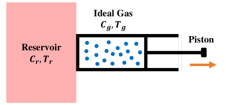
Figure 1: Schematic diagram of the gas-reservoir system. $T_{r}$ ($T_{g}$) and $C_{r}$ ($C_{g}$) are the temperature and heat capacity at constant volume of the reservoir (gas), respectively.

Noticing that the internal energy change of the ideal gas $dU_{g}=C_{g}dT$ with the heat capacity of the gas $C_{g}$, and $\delta Q_{g}=-\delta Q_{r}$, we can rewrite Eq. (1) as

$$\delta Q_{g}=C_{g}dT+PdV=-C_{r}dT.$$ (3)

By substituting the ideal gas equation into Eq. (3), we obtain the following differential equation

$$\left(C_{g}+C_{r}\right)dT=-PdV=-\frac{Nk_{B}T}{V}dV,$$ (4)

with the number of gas particle $N$ and the Boltzmann constant $k_{B}$. With the assumption that the reservoir has constant heat capacity, the solution of Eq. (4) is straightforward obtained as

$$TV^{\left(\frac{\gamma-1}{1+C_{r}/C_{g}}\right)}=\mathrm{const},$$ (5)

where $\gamma\equiv 1+Nk_{B}/C_{g}$ is the heat capacity ratio of the ideal gas. The above equation can be re-written in terms of $P$ and $V$ as

$$PV^{\xi}=\mathrm{const},\;\xi\equiv\frac{\gamma+C_{r}/C_{g}}{1+C_{r}/C_{g}}.$$ (6)

Arrive here, the polytropic process equation is derived from our simple model, and we see that the polytropic exponent $\xi$ is determined by the heat capacity ratio between the reservoir and gas. As an illustration, the $P-V$ diagram of the diatomic molecule gas ($\gamma=1.4$) with different $C_{r}/C_{g}$ is plotted in Fig. 2. In addition, from the perspective of potential application, if the heat capacity of the reservoir is unknown, with the polytropic exponent obtained by measuring the $P-V$ diagram of the gas, Eq. (6) indicates that the heat capacity of the reservoir can be estimated as $C_{r}=C_{g}(\gamma-\xi)/(\xi-1)$.

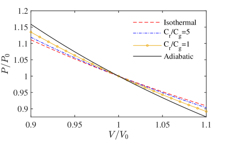
Figure 2: $P-V$ diagram of the gas with different $C_{r}/C_{g}$. The blue dash-dotted curve and yellow circled curve are plotted with $C_{r}/C_{g}=5$ and $C_{r}/C_{g}=1$, respectively. The red dashed curve represents the isothermal thermal process ($C_{r}\rightarrow\infty$) while the black solid curve represents the adiabatic process ($C_{r}\rightarrow 0$). $P_{0}$ ($V_{0}$) is the initial gas pressure (volume) for a given process. In this example, we use $\gamma=1.4$.

We further analyze the obtained polytropic process equation in different limits of $C_{r}$ with given $C_{g}$:

i) In the limit that the reservoir size tends to infinity with $C_{r}\rightarrow\infty$, one has $\xi\rightarrow 1$, and thus $T=\mathrm{const}$, which means the process becomes an isothermal process (red dashed curve in Fig. 2). This result is very intuitive, because when the heat capacity of the reservoir tends to infinity, its temperature change tends to 0 correspondingly, that is, the reservoir becomes a heat bath with constant temperature.

ii) In the limit of $C_{r}\rightarrow 0$, the reservoir can be considered as disappearing, such that the gas becomes an isolated system with $\xi\rightarrow\gamma$. In this case, Eq. (5) recovers the adiabatic equation of ideal gas $PV^{\gamma}=\mathrm{const}$, which is represented by the black solid curve in Fig. 2.

It is worth mentioning that, conventional materials generally have positive heat capacity ($C_{r}>0$), and thus $C_{r}/C_{g}\in(0,\infty)$. In this case, the polytropic exponent $\xi\in(1,\gamma)$, which result in Eq. (6) can not describe the isochoric process ($\xi\rightarrow\infty$) and the isobaric process ($\xi\rightarrow 0$). Interestingly, it is easy to check that the process equations of these two typical processes can be covered by Eq. (6) once the reservoir’s heat capacity can take negative values . The requirement that the reservoir has negative heat capacity can be achieved with unconventional materials (Schmidt et al., 2001; Ma, 2020) or by applying work on the reservoir , which will not be discussed in detail here.

Work and heat.– Considering the volume of the gas with initial temperature $T_{0}$ is tuned from $V_{0}$ to $V_{f}$ in the discussed process, it follows from Eq. (5) that the final temperature of the gas is

$$T_{f}=T_{0}\left(\frac{V_{0}}{V_{f}}\right)^{\xi-1}\equiv T_{0}\mathrm{e}^{-\lambda\kappa}$$ (7)

with $\lambda=\ln(V_{f}/V_{0})$ and $\kappa=\xi-1=(\gamma-1)/(1+C_{r}/C_{g})$. According to Eq. (4), the output work of the gas is,

$$W =\int_{V_{0}}^{V_{f}}PdV=-\left(C_{g}+C_{r}\right)\int_{T_{0}}^{T_{f}}dT$$ (8)

$$=\left(C_{g}+C_{r}\right)T_{0}\left(1-\mathrm{e}^{-\lambda\kappa}\right).$$ (9)

In addition, it follows from Eq. (3) that the heat absorbed of the gas

$$Q_{g}=-C_{r}\int_{T_{0}}^{T_{f}}dT=\frac{C_{r}}{C_{g}+C_{r}}W,$$ (10)

which is proportional to the output work. This is in consistent with a recent study on the polytropic process (Christians, 2012), where the authors defined the energy transfer ratio $\delta Q_{g}/\delta W\equiv K$ and introduced a basic assumption that $K$ is a constant.

When the heat capacity of the reservoir is much lager than that the gas, i.e., $C_{g}\ll C_{r}$, keeping to the first order of $\kappa$ or $C_{g}/C_{r}$, the output work in Eq. (9) is approximated as

$$W =\frac{Nk_{B}}{\kappa}T_{0}\left\{1-\left[1-\lambda\kappa+\frac{1}{2}\lambda^{2}\kappa^{2}+O\left(\kappa^{3}\right)\right]\right\}$$ (11)

$$\approx Nk_{B}T_{0}\left(\lambda-\frac{1}{2}\lambda^{2}\kappa\right)$$ (12)

$$\approx W_{\mathrm{iso}}\left(1-\frac{\gamma-1}{2C_{r}/C_{g}}\right),$$ (13)

where $W_{\mathrm{iso}}\equiv Nk_{B}T_{0}\ln(V_{f}/V_{0})$ is the output work of the gas in the isothermal process with temperature $T_{0}$. The second term in Eq. (13) is the correction due to the finiteness in size of the reservoir, which will reduce the amount of output work compared to $W_{\mathrm{iso}}$ in the case with infinite heat reservoir. This $1/C_{r}$ correction agrees well with some recent studies on finite-system thermodynamics and statistics (Reeb and Wolf, 2015; Richens et al., 2018; Timpanaro et al., 2020; Ma et al., 2021)

Conclusion and discussions.– The simple gas-reservoir model proposed in this paper can deepen students’ understanding of the polytropic process and can be directly extended to the van der Waals gas system (Malic, 1955).

In common sense, the thermal reservoir is generally considered as a thermal equilibrium system with infinite degrees of freedom, and the temperature is its only characteristic quantity. Correction related to the finiteness of the reservoirs in the energy conversion process will lead students to think about the novel thermodynamic effects off the thermodynamic limit (Ondrechen et al., 1981; Leff, 1987; Ma, 2020; Ma et al., 2021; Yuan et al., 2022). When the heat capacity of the thermal reservoir is temperature -dependent, the solution of Eq. (4) will no longer satisfy the polytropic process equation, the $P-V$ diagram of the gas in this case is worth further exploring. Moreover, without the quasi-static assumption, taking into account the non-equilibrium heat transfer, this model can also be utilized to study the irreversible thermodynamic behavior of the gas driven in finite time (Curzon and Ahlborn, 1975; Andresen, 1983; den Broeck, 2005; Ma et al., 2020, 2018).

As a final remark, it is feasible in principle to experimentally demonstrate our model at the undergraduate level. For example, when the ideal gas is specific as $10$L of air ($C_{g}\approx\mathrm{9.3J/K,\gamma\approx 1.4})$ around the zoom temperature, a) if the reservoir is 2L of air ($C_{r}\approx\mathrm{1.86J/K})$, according to Eq. (5), the polytropic exponent $\xi\approx 1.333$; b) if the reservoir is also$10$L of air, the polytropic exponent $\xi\approx 1.2$; c) if the reservoir is specific as a cup of water ($200$mL, $C_{r}\approx\mathrm{840J/K}$), the polytropic exponent $\xi\approx 1.004$, which means the designed process is very close to an isothermal process. The $P-V$ diagram of the air in the whole process can be obtained by directly measuring the volume and pressure of the air (Ma et al., 2020). Apart from exchanging heat with each other, isolating the gas and the reservoir from the outside environment to avoid extra heat dissipation is the main difficulty of this experiment.

Acknowledgments.– The author would like to thank Shi-Gang Ou, Shan-He Su, Tao Li and Hong Yuan for valuable comments on the manuscript. This work is supported by the National Natural Science Foundation of China (Grants No. 12088101, No. U1930402, and No. U1930403), and the China Postdoctoral Science Foundation (Grant No. BX2021030).

References

- Callen (1960) H. B. Callen, Thermodynamics and an Introduction to Thermostatistics (John Wiley & Sons, New York, 1960).
- Cengel et al. (2011) Y. A. Cengel, M. A. Boles, and M. Kanoğlu, Thermodynamics: an engineering approach, vol. 5 (McGraw-hill New York, 2011).
- Note (1) Note1, result in while is achieved with .
- Schmidt et al. (2001) M. Schmidt, R. Kusche, T. Hippler, J. Donges, W. Kronmüller, B. Von Issendorff, and H. Haberland, Phys. Rev. Lett. 86, 1191 (2001).
- Ma (2020) Y.-H. Ma, Entropy 22, 1002 (2020).
- Note (2) Note2, considering that the work is applied to the reservoir through a generalized force conjugated to the generalized displacement as , the law of energy conservation for the reservoir in this situation reads . The heat capacity of the reservoir follows as , which can be negative when .
- Christians (2012) J. Christians, International Journal of Mechanical Engineering Education 40, 53 (2012).
- Reeb and Wolf (2015) D. Reeb and M. M. Wolf, IEEE Transactions on Information Theory 61, 1458 (2015).
- Richens et al. (2018) J. G. Richens, Á. M. Alhambra, and L. Masanes, Phys. Rev. E 97, 062132 (2018).
- Timpanaro et al. (2020) A. M. Timpanaro, J. P. Santos, and G. T. Landi, Phys. Rev. Lett. 124, 240601 (2020).
- Ma et al. (2021) Y.-H. Ma, C. L. Liu, and C. P. Sun, arXiv:2110.04550 (2021).
- Malic (1955) D. Malic, Journal of the Franklin Institute 259, 235 (1955).
- Ondrechen et al. (1981) M. J. Ondrechen, B. Andresen, M. Mozurkewich, and R. S. Berry, Am. J. Phys. 49, 681 (1981).
- Leff (1987) H. S. Leff, Am. J. Phys. 55, 701 (1987).
- Yuan et al. (2022) H. Yuan, Y.-H. Ma, and C. Sun, Phys. Rev. E 105, L022101 (2022).
- Curzon and Ahlborn (1975) F. L. Curzon and B. Ahlborn, Am. J. Phys. 43, 22 (1975).
- Andresen (1983) B. Andresen, Finite-time thermodynamics (University of Copenhagen Copenhagen, 1983).
- den Broeck (2005) C. V. den Broeck, Phys. Rev. Lett. 95, 190602 (2005).
- Ma et al. (2020) Y.-H. Ma, R.-X. Zhai, J. Chen, H. Dong, and C. P. Sun, Phys. Rev. Lett. 125, 210601 (2020).
- Ma et al. (2018) Y.-H. Ma, D. Xu, H. Dong, and C.-P. Sun, Phys. Rev. E 98, 042112 (2018).