Structural aspects of FRG in quantum tunnelling computations

Abstract

ABSTRACT

We probe both the unidimensional quartic harmonic oscillator and the double well potential through a numerical analysis of the Functional Renormalization Group flow equations truncated at first order in the derivative expansion. The two partial differential equations for the potential $V_{k}(\varphi)$ and the wave function renormalization $Z_{k}(\varphi)$, as obtained in different schemes and with distinct regulators, are studied down to $k=0$, and the energy gap between lowest and first excited state is computed, in order to test the reliability of the approach in a strongly non-perturbative regime. Our findings point out at least three ranges of the quartic coupling $\lambda$, one with higher $\lambda$ where the lowest order approximation is already accurate, the intermediate one where the inclusion of the first correction produces a good agreement with the exact results and, finally, the one with smallest $\lambda$ where presumably the higher order correction of the flow is needed. Some details of the specifics of the infrared regulator are also discussed.

I Introduction

In spite of the enormous success of functional renormalization group (FRG) approach in statistical mechanics and quantum field theory (see Dupuis et al. (2021) for a recent review), its applicability to strongly non-perturbative problems is not obvious. In particular, the calculation of the energy gap $\Delta E$ between the first excited state and the ground state for the anharmonic oscillator is an important test to study the effectiveness of the FRG approach to capture genuine topological effects. This model is based on the one particle Hamiltonian with potential (here $\varphi$ indicates the coordinate of the particle) :

$$V(\varphi)=\frac{M^{2}}{2}\;\varphi^{2}+\lambda\varphi^{4}$$ (1)

which corresponds to the anharmonic oscillator with quartic corrections if $M^{2}>0$, or to the double well potential if $M^{2}<0$. In the following, we express all dimensionful quantities in terms of the square mass scale $|M^{2}|$, which is equivalent to choose either $M^{2}=1$ or $M^{2}=-1$.

In the former case, a quartic term is added to the exactly solvable harmonic oscillator Hamiltonian, and therefore a perturbative treatment of the problem is suitable as long as the quartic coupling does not grow too large. In the latter case, the quadratic part is unstable and the stabilizing quartic term produces a double well that becomes deeper and deeper when $\lambda\to 0$. This means that the effect of the tunnelling of the wave function becomes more important for $\lambda\to 0$, and therefore in this limit any perturbative approach fails to produce reasonable results.

A reliable approach to confront the $M^{2}=-1$, $\lambda\to 0$ problem is the dilute instanton gas calculation Coleman (1985); Zinn-Justin (2002) that produces the well known, non-analytic exponential expression of the energy gap $\Delta E$ between first excited and ground state

$$\Delta E_{inst}=2\;\Biggl{(}\frac{2\sqrt{2}}{\pi\lambda}\Biggr{)}^{1/2}\;{\rm e}^{-\,{\left(3\lambda\sqrt{2}\right)^{-1}}}$$ (2)

Clearly, the quantum mechanical problem, either with $M^{2}=1$ or $M^{2}=-1$, can be solved through the numerical determination of the eigenvalues of the associated Scröedinger equation which then provides the exact reference values of $\Delta E_{exact}$ at each value of $\lambda$.

Consequently, the calculation of $\Delta E$ represents an important challenge for the FRG approach, in particular for low values of $\lambda$. Moreover, this analysis can be regarded as an essential step toward the application of the FRG to more complex problems regarding the estimate of false vacuum decay rates in quantum field theoryDevoto et al. (2022) and, more specifically, concerning the stability of the electroweak vacuum, related to the Ultraviolet (UV) completion of the Standard Model, and the study of inflationary models in cosmology Bezrukov and Shaposhnikov (2008), because in these contexts the typical approach adopted mainly relies on instanton calculation (see e.g. Bentivegna et al. (2017); Branchina et al. (2019)).

Early works started the investigation of this problem by means of a sharp cut-off FRG in the local potential approximation (LPA), either within a polynomial truncation of the resulting flow equation for the potential Horikoshi et al. (1998); Aoki et al. (2002), or by direct numerical resolution of the local potential flow equation Kapoyannis and Tetradis (2000). The inclusion of a field dependent wave-function renormalization $Z(\phi)$ first appeared in Zappala (2001) by means of a Schwinger’s proper-time cutoff in the FRG equation. In that work a numerical integration of the combined system of non-linear parabolic Partial Differential Equations (PDE) for the local potential $V(\phi)$ and $Z(\phi)$ was employed.

In fact, polynomial truncations of the FRG generate a system of differential equations which is singular in the $k\rightarrow 0$ limit in the broken phase. On the contrary, the full set of PDE correctly reproduces the discontinuity in the correlation length below the critical temperature Parola et al. (1993) but the numerical integration is not straightforward, as one has to resort to implicit methods for a class of coupled non-linear parabolic evolution equation Bonanno and Lacagnina (2004); Caillol (2012). In $d=1$ dimensions the evolution of flow in the infrared is less severe and one can hope that already with the familiar method of the lines (MoL) Ames et al. (1977), it is possible to reach values of $\lambda$ small enough to render the comparison with standard dilute instanton gas approach meaningful. In Weyrauch (2006), FRG with smooth and sharp cut-off have been solved with both polynomial truncation and MoL but some discrepancies between the findings of Weyrauch (2006) and Zappala (2001) for very small $\lambda$ have emerged. Further applications of FRG to supersymmetric quantum mechanics have appeared in Synatschke et al. (2009). An attempt to apply the Principle of Minimal Sensitivity in this context has recently been discussed in Kovacs et al. (2015).

Beyond LPA a number of structural aspects in the formulation of FRG arise. In the case of the so called spectrally adjusted (SA) flow the coarse-graining procedure is built in terms of the eigenvalues of the spectrum of $\Gamma_{k}^{(2)}$ evaluated at the background field Gies (2002), where $\Gamma_{k}$ is the effective average action at the scale $k$. The spectrum is therefore not fixed but computed at the running cutoff $k$. If we visualize the averaging procedure in real space, the use of a running cutoff built with a running blocked field can be thought as the analogous of a ”lagrangian” description of the dynamic of the fluid made by a co-moving observer. On the contrary the ”eulerian” coarse-grainined flow is produced if, in lowering the cutoff from $k$ to $k-\Delta k$, a fixed spectrum of the Laplacian operator $\Box$ is employed at each $k$. Clearly both ”lagrangian” and ”eulerian” schemes lead to very similar results near criticality when the anomalous dimension is small, but it is not clear which scheme is to be expected to work better in general.

From this point of view we would like to stress that, strictly speaking, only FRG with not spectrally adjusted (NSA) regulators are ”exact” flow in the sense of Wetterich (1993); Morris (1994), while SA regulators, albeit widely used in the FRG literature, are not in general exact unless they are derived from a much more involved and non-linear flow equation which we will not consider in this paper Litim and Pawlowski (2002a).

The aim of this work is twofold. First, we would like to address the computation of $\Delta E$ in the small $\lambda$ regime, by means of distinct formulations, namely the Exact Renormalization Group (ERG) flow equations characterized by the theta-function regulator proposed in Litim (2000) and the Schwinger’s Proper Time (PT) flow equations introduced in Bonanno and Zappala (2001); Bonanno and Reuter (2005); de Alwis (2018), in order to get an inclusive prediction of $\Delta E$ from the FRG. This point is essential both to test the reliability of this approach in the deep non-perturbative regime ($\lambda<<1$), especially in comparison with the instanton gas calculation, and, at the same time, to produce a countercheck on the mentioned discrepancy with the analysis of Weyrauch (2006). Second, we intend to study the impact of SA vs. NSA cutoff in the low $\lambda$ region for these type of FRG. In particular, in the case of the PT flow, we further discuss the dependence of the various cutoff schemes introduced in Bonanno et al. (2020).

The structure of the paper is the following. In Sect. II we review the structure of the flow equations that are subsequently integrated and, more specifically, Sect. II.1 is devoted to the ERG flow, while in Sect. II.2 the PT equations are discussed. Then, in Sect. III the results of our numerical analysis are presented, first considering the LPA approximation in III.2, and by including the wave function renormalization in III.3. Our conclusions are reported in Sect. IV.

II Flow equations

II.1 ERG flow

We shall first consider the implementation of the ERG flow Dupuis et al. (2021) (we define the RG ’time’as $t=\log(k/\Lambda)$, where $k$ is the running energy scale and $\Lambda$ is a fixed UV cutoff)

$$\partial_{t}\Gamma_{k}[\varphi]=\frac{1}{2}{\rm Tr}\Bigl{[}\partial_{t}{R}_{k}(q^{2})\;G_{k}(q^{2},\varphi)\Bigr{]}$$ (3)

and the regularized propagator $G_{k}(q^{2},\varphi)$ is

$$G_{k}(q^{2},\varphi)=\frac{1}{\Gamma^{(2)}_{k}(q^{2},\varphi)+R_{k}(q^{2})}=\frac{1}{Z_{k}(\varphi)\,q^{2}+V^{\prime\prime}_{k}(\varphi)+R_{k}(q^{2})}\;.$$ (4)

$R_{k}(q^{2})$ is the regulator of the infrared modes which will be specified below. $\Gamma^{(2)}_{k}(q^{2},\varphi)$ indicates the second functional derivative of $\Gamma_{k}[\varphi]$ with respect to the field $\varphi$. Here and below, prime, double prime, etc. indicate one, two, etc. derivatives with respect to the argument.

The explicit form adopted for the running effective action $\Gamma_{k}[\varphi]$ comes from the first non trivial order of its derivative expansion:

$$\Gamma_{k}[\varphi]=\int{\rm d}^{d}x\left[V_{k}(\varphi)+\frac{1}{2}Z_{k}(\varphi)(\partial\varphi)^{2}\right]+O(\partial^{4})$$ (5)

and we focus on the flows of $V_{k}$ and $Z_{k}$, which are derived from the flow of the two-point function

$$\partial_{t}\Gamma_{k}^{(2)}(p^{2})\;\;=\;\;\partial_{t}Z_{k}\,p^{2}+\partial_{t}V^{\prime\prime}_{k}\;\;=$$

$$\int_{q}\left[\Gamma_{k}^{(3)}(q,p,-q-p)\right]^{2}G_{k}\big{(}(q+p)^{2}\big{)}G_{k}^{2}(q^{2})\partial_{t}{R}_{k}(q^{2})-\frac{1}{2}\int_{q}\Gamma_{k}^{(4)}(q,p,-p,-q)G_{k}^{2}(q^{2})\partial_{t}{R}_{k}(q^{2})=$$

$$\int_{q}\left[Z^{\prime}_{k}\left(q^{2}+q\cdot p+p^{2}\right)+V^{\prime\prime\prime}_{k}\right]^{2}G_{k}\big{(}(q+p)^{2}\big{)}G_{k}^{2}(q^{2})\partial_{t}{R}_{k}(q^{2})$$

$$-\frac{1}{2}\int_{q}\left[Z^{\prime\prime}_{k}\left(q^{2}+p^{2}\right)+V^{\prime\prime\prime\prime}_{k}\right]G_{k}^{2}(q^{2})\partial_{t}{R}_{k}(q^{2})$$ (6)

by respectively extracting the $O(p^{0})$ and $O(p^{2})$ coefficients in the expansion of the left hand side (lhs) of Eq. (6) in powers of momentum $p$. Incidentally, we notice that in Eq. (6) the symmetry $\Gamma_{k}^{(3)}(q,p,-q-p)=\Gamma_{k}^{(3)}(q+p,-p,-q)$ is used to simplify the first contribution (diagram).

Therefore, we need to expand the propagator $G_{k}\big{(}{\tiny(q+p)^{2}}\big{)}$ in Eq. (6), in powers of $p$

$$G_{k}\big{(}{\tiny(q+p)^{2}}\big{)}=G_{k}(q^{2})+2xq\,G^{\prime}_{k}(q^{2})p+\bigl{[}G^{\prime}_{k}(q^{2})+2x^{2}q^{2}G^{\prime\prime}_{k}(q^{2})\bigr{]}p^{2}+O(p^{3}))\,.$$ (7)

where we recall that primes indicate derivative with respect to the argument and we labelled the cosine of the angle between the four-vectors $p$ and $q$, as $x$.

Then, by definition, the derivatives of the regularized propagator are

$$G^{\prime}_{k}=-G^{2}_{k}(Z_{k}+R^{\prime}_{k})\qquad\qquad G^{\prime\prime}_{k}=2G^{3}_{k}(Z_{k}+R^{\prime}_{k})^{2}-G^{2}_{k}R^{\prime\prime}_{k}$$ (8)

and we can insert Eqs. (7), (8) into Eq. (6), to obtain the flow equations for $V_{k}$ and $Z_{k}$

$$\partial_{t}V_{k}=\mathcal{B}_{V}^{d}\!\left(V_{k}^{\prime\prime},Z_{k}\right)\qquad\qquad\partial_{t}Z_{k}=\mathcal{B}_{Z}^{d}\!\left(V_{k}^{\prime\prime},V_{k}^{\prime\prime\prime},Z_{k},Z_{k}^{\prime},Z_{k}^{\prime\prime}\right)$$ (9)

where the explicit expressions for the right hand side (rhs) are

$$(4\pi)^{\frac{d}{2}}\,\mathcal{B}_{V}^{d}=\frac{1}{2}Q_{\frac{d}{2}}\!\left[G_{k}\partial_{t}R_{k}\right]$$ (10)

and

$$(4\pi)^{\frac{d}{2}}\,\mathcal{B}_{Z}^{d}\;\;\;\;= \left(V_{k}^{\prime\prime\prime}\right)^{2} \left\{Q_{\frac{d}{2}}\left[G_{k}^{2}G_{k}^{\prime}\partial_{t}R_{k}\right]+Q_{\frac{d}{2}+1}\left[G_{k}^{2}G_{k}^{\prime\prime}\partial_{t}R_{k}\right]\right\}$$ (11)

$$+Z_{k}^{\prime}V_{k}^{\prime\prime\prime} \left\{2Q_{\frac{d}{2}}\left[G_{k}^{3}\partial_{t}R_{k}\right]+(d+2)Q_{\frac{d}{2}+1}\left[G_{k}^{2}G_{k}^{\prime}\partial_{t}R_{k}\right]\right.$$

$$\;\;\left.+(d+2)Q_{\frac{d}{2}+2}\left[G_{k}^{2}G_{k}^{\prime\prime}\partial_{t}R_{k}\right]\right\}$$

$$+\left(Z_{k}^{\prime}\right)^{2} \left\{\frac{2d+1}{2}Q_{\frac{d}{2}+1}\left[G_{k}^{3}\partial_{t}R_{k}\right]+\frac{(d+2)(d+4)}{4}Q_{\frac{d}{2}+2}\left[G_{k}^{2}G_{k}^{\prime}\partial_{t}R_{k}\right]\right.$$

$$\;\;\left.+\frac{(d+2)(d+4)}{4}Q_{\frac{d}{2}+3}\left[G_{k}^{2}G_{k}^{\prime\prime}\partial_{t}R_{k}\right]\right\}$$

$$+\;Z_{k}^{\prime\prime} \left\{-\frac{1}{2}Q_{\frac{d}{2}}\left[G_{k}^{2}\partial_{t}R_{k}\right]\right\}$$

and the $Q$–functionals of variable $z=q^{2}$ are defined as:

$$Q_{n}[f]\equiv\frac{1}{\Gamma[n]}\int_{0}^{\infty}\,dz\,z^{n-1}f(z)$$ (12)

So far, all relations are valid for an arbitrary cutoff function and in any dimension. Now, we specify the function $R_{k}(z)$ by taking Litim’s regulator Litim (2000), in two different forms, namely in the plain NSA version

$$R^{NSA}_{k}(z)=(k^{2}-z)\,\theta(k^{2}-z)$$ (13)

and in the SA form that includes a field dependent wave-function renormalization prefactor

$$R^{SA}_{k}(z)=Z_{k}(\varphi)\,(k^{2}-z)\,\theta(k^{2}-z)\,,$$ (14)

and $\theta(x)$ is the Heaviside function.

In the NSA case, only a partial cancellation of the square momentum $z$ dependence of $G_{k}(z)$ is realized, with the residual dependence weighted by the deviation of the factor $Z_{k}(\varphi)$ from 1 :

$$G_{k}(z)=\frac{1}{Z_{k}\,z+(k^{2}-z)\theta(k^{2}-z)+V^{\prime\prime}_{k}}$$ (15)

and the replacement of Eqs. (13), (15) into Eqs. (12), (10) and (11) leads us to a coupled pair of flow equations for $V_{k}$ and $Z_{k}$, where the integration over the variable $z$ in Eq. (12) produces a long and involved sum of Hypergeometric functions, due to the not full momentum simplification in Eq. (15). Still, in this case, it is possible to recover an explicit, analytic form, suitable for numerical integration (which is discussed in the next Section), of the partial differential equations (PDE) governing the flow of $V_{k}$ and $Z_{k}$, that, for the sake of simplicity, we do not display here.

The SA regulator displayed in (14) instead produces a much simpler structure of the flow equations, thanks to the presence of $Z_{k}(\varphi)$ in $R^{SA}_{k}(z)$. In fact, in this case the propagator reduces to the square momentum $z$ independent quantity ${H_{k}}^{-1}(\varphi)$ :

$$G_{k}(z)=\frac{1}{Z_{k}z+Z_{k}(k^{2}-z)\theta(k^{2}-z)+V^{\prime\prime}_{k}}\;\to\;\frac{1}{Z_{k}k^{2}+V^{\prime\prime}_{k}}\;\equiv\;\frac{1}{H_{k}}$$ (16)

and the corresponding $Q$–functionals entering $\mathcal{B}_{V}^{d}$ and $\mathcal{B}_{Z}^{d}$, have the following simple form:

$$Q_{n}[G_{k}^{m}\partial_{t}R_{k}]=\frac{k^{2(n-m+1)}}{\Gamma(n)}\frac{Z_{k}}{(Z_{k}+\omega_{k})^{m}}\left\{\frac{2-\eta_{k}}{n}+\frac{\eta_{k}}{n+1}\right\}$$ (17)

$$Q_{n}[G_{k}^{m}G^{\prime}_{k}\partial_{t}R_{k}]=0$$ (18)

$$Q_{n}[G_{k}^{m}G_{k}^{\prime\prime}\partial_{t}R_{k}] = -\frac{k^{2(n-m-2)}}{\Gamma(n)}\frac{Z_{k}^{2}}{(Z_{k}+\omega_{k})^{m+2}}$$ (19)

where we used the specific value of Heaviside function at the origin, $\theta(0)=1/2$, and we defined $\omega_{k}\equiv V^{\prime\prime}_{k}/k^{2}$ and the field and scale dependent $\eta_{k}(\varphi)$ (recall $t=\log(k/\Lambda)$) as

$$\eta_{k}(\varphi)\equiv-\partial_{t}\log Z_{k}(\varphi)\;,$$ (20)

that must not be mistaken for the field anomalous dimension at criticality. Then for the SA case, Eqs. (14), (17), (18), (19), and (16) yield the following $\mathcal{B}$-functions in $d=1$, to be inserted in Eq. (10)

$$\mathcal{B}_{V}^{d=1}=\frac{Z_{k}k^{3}}{\pi\,H_{k}}\;\left(1-\eta_{k}/3\right)$$ (21)

$$\mathcal{B}_{Z}^{d=1}=\;\frac{Z_{k}k^{3}}{\pi\,H_{k}} \cdot \Bigg{\{}\left(-\frac{Z^{\prime\prime}_{k}}{H_{k}}\,+\,\frac{4\,Z^{\prime}_{k}V^{\prime\prime\prime}_{k}}{H_{k}^{2}}\,\right)\left(1-\frac{\eta_{k}}{3}\right)\,+\,\frac{2\,(Z^{\prime}_{k})^{2}\,k^{2}}{H_{k}^{2}}\,\left(1-\frac{\eta_{k}}{5}\right)$$

$$- \,\frac{Z_{k}(V^{\prime\prime\prime}_{k})^{2}}{H_{k}^{3}}\,-\,\frac{2k^{2}\,Z_{k}Z^{\prime}_{k}V^{\prime\prime\prime}_{k}}{H_{k}^{3}}\,-\,\frac{Z_{k}\,(Z^{\prime}_{k})^{2}\,k^{4}}{H_{k}^{3}}\Bigg{\}}$$ (22)

Despite the compact form of the flow equations displayed in Eqs. (21) and (II.1), we notice that terms proportional to $\eta_{k}$ introduce nonlinear effects related to the ’time’ derivative of $Z_{k}$, which are harmless as long as $Z_{k}\simeq 1$, but become very difficult to handle in the numerical integration when $Z_{k}$ becomes substantially different from 1, which occurs in the region of very small coupling $\lambda$ in Eq. (1). Due to this complication, together with the full flow of $V_{k}$ and $Z_{k}$ in Eqs. (21) and (II.1), we shall analyze its reduced version obtained by simply setting $\eta_{k}=0$, thus making the flow equations linear both in $\partial_{t}V_{k}$ and $\partial_{t}Z_{k}$, and therefore much easier to integrate numerically.

II.2 Proper Time flow

Now, we turn to a different kind of flow, namely the Proper Time (PT) flow, whose equations for $V_{k}$ and $Z_{k}$ can be cast in the form of PDE, suitable for numerical investigation. This kind of flow is to be regarded as a particular case of background field flow Litim and Pawlowski (2002b), although recently it was reconsidered as a type of Wilsonian action flow de Alwis (2018); Bonanno et al. (2020), and the corresponding flow equations of $V_{k}$ and $Z_{k}$ are discussed in detail in Bonanno et al. (2020). Here, we do not focus on the nature of the PT flow, as we are rather interested in its application to the spectrum of the double well potential and we refer to Bonanno et al. (2020) for a detailed discussion on the structure of the regulator and on the consequent derivation of the flow equations, both in the NSA and in the SA case.

Here, we just mention that the NSA regulator, which carries no dependence on the renormalization factor $Z_{k}$, produces the following flow equation (named ”A-scheme” in Bonanno et al. (2020))

$$\partial_{t}\Gamma_{k}[\varphi]=-{\rm Tr}\left(\frac{mk^{2}}{\Gamma^{(2)}_{k}[\varphi]+mk^{2}}\right)^{m}.$$ (23)

where $m>d/2$ is a free parameter that roughly specifies the sharpness of the regulator, and it is usually taken as integer. Eq. (23) in $d=1$ and with the same formal parameterization of the action adopted in Eq. (5), reduces to the following NSA coupled flow

$$\partial_{t}V_{k}=-\;\frac{\Gamma(m-1/2)}{2\;\sqrt{\pi}\;\Gamma(m)}\;\,\sqrt{\frac{m\,k^{2}}{Z_{k}}}\;\;\left(\frac{\;m\;k^{2}\;}{\;\;h^{{}^{NSA}}_{k,\,m}\;\;}\right)^{m-1/2}$$ (24)

$$\partial_{t}Z_{k} = \;\frac{\Gamma(m+1/2)}{2\;\sqrt{\pi}\;\Gamma(m)}\;\,\sqrt{\frac{m\,k^{2}}{Z_{k}}}\;\;\left(\frac{\;m\;k^{2}\;}{\;\;h^{{}^{NSA}}_{k,\,m}\;\;}\right)^{m-1/2}\cdot$$ (25)

$$\left[\;\frac{Z^{\prime\prime}_{k}}{h^{{}^{NSA}}_{k,\,m}}+\frac{Z_{k}(V^{\prime\prime\prime}_{k})^{2}(m+1/2)(m+3/2)}{6\left(h^{{}^{NSA}}_{k,\,m}\right)^{3}}-\frac{3\,Z^{\prime}_{k}V^{\prime\prime\prime}_{k}(m+1/2)}{2\left(h^{{}^{NSA}}_{k,\,m}\right)^{2}}\,-\,\frac{21}{24}\,\frac{(Z^{\prime}_{k})^{2}}{Z_{k}\,h^{{}^{NSA}}_{k,\,m}}\right]$$

where $\Gamma(x)$ is the Gamma-function and $h^{{}^{NSA}}_{k,m}$ is

$$h^{{}^{NSA}}_{k,\,m}=m\,k^{2}+V_{k}^{\prime\prime}$$ (26)

On the other hand, the SA flow requires the replacement of the scale $k^{2}$ with the corrected scale $Z_{k}(\varphi)\;k^{2}$ in the regulator and this produces flow equations indicated in Bonanno et al. (2020) as the ’B-scheme’, or as the ’simplified type-C scheme’ if the derivatives of the factors $Z_{k}(\varphi)$ that appear in the regulator are neglected. We refer to Bonanno et al. (2020) for the explicit involved form of the flow equations of $V_{k}$ and $Z_{k}$ in the ’B-scheme’, while the ’simplified type-C scheme’ equations are simply obtained from Eqs. (24) and (25) by replacing everywhere $m\;k^{2}\;\to\;Z_{k}(\varphi)\,m\;k^{2}$, i.e. we find

$$\partial_{t}V_{k}=\,-\;\frac{\Gamma(m-1/2)}{2\;\sqrt{\pi}\;\Gamma(m)}\;\,\sqrt{m\,k^{2}}\;\;\left(\frac{Z_{k}\;m\;k^{2}\;}{\;\;h^{{}^{SA}}_{k,\,m}\;\;}\right)^{m-1/2}$$ (27)

$$\partial_{t}Z_{k} = \;\frac{\Gamma(m+1/2)}{2\;\sqrt{\pi}\;\Gamma(m)}\;\,\sqrt{m\,k^{2}}\;\;\left(\frac{Z_{k}\;m\;k^{2}\;}{\;\;h^{{}^{SA}}_{k,\,m}\;\;}\right)^{m-1/2}\cdot$$ (28)

$$\left[\;\frac{Z^{\prime\prime}_{k}}{h^{{}^{SA}}_{k,\,m}}+\frac{Z_{k}(V^{\prime\prime\prime}_{k})^{2}(m+1/2)(m+3/2)}{6\left(h^{{}^{SA}}_{k,\,m}\right)^{3}}-\frac{3\,Z^{\prime}_{k}V^{\prime\prime\prime}_{k}(m+1/2)}{2\left(h^{{}^{SA}}_{k,\,m}\right)^{2}}\,-\,\frac{21}{24}\,\frac{(Z^{\prime}_{k})^{2}}{Z_{k}\,h^{{}^{SA}}_{k,\,m}}\right]$$

with the definition

$$h^{{}^{SA}}_{k,\,m}\equiv Z_{k}\;m\,k^{2}+V_{k}^{\prime\prime}\;.$$ (29)

We notice that the ’simplified type-C scheme’ flow equations (27) and (28) are equal to the pair of equations analyzed in Zappala (2001) (and previously introduced in Bonanno and Zappala (2001)), provided that the scale $\hat{k}$ and the parameter $\hat{m}$, used in Zappala (2001), are replaced with our $k$ and $m$, according to $\hat{m}+1=m$ and $\hat{k}=k\,m/\hat{m}$. Clearly, observables calculated in the limit $k\to 0$ are insensible to the difference between $k$ and $\hat{k}$, and one can compare the results derived from the two flows for equivalent values of $m$ and $\hat{m}$.

Computations in Zappala (2001) were performed with a particular exponential form of the flow obtained in the limit $\hat{m}\to\infty$. In fact, the same exponential flow equations are recovered from Eqs. (27) and (28) in the limit $m\to\infty$; however we shall not repeat here the computation of $\Delta E$ in this case, but rather look at the PT flow at the reasonably large value $m=10$, to produce predictions close to those of the exponential flow.

In addition, we notice that the SA version of the PT flow in Eqs. (27) and (28) at the particular value $m=3/2$, resembles the ERG displayed in Eqs. (21) and (II.1), at $\eta_{k}=0$. Actually, for $m=3/2$, the flow equations for $V_{k}$ (27) and (21) coincide, while in the equations for $Z_{k}$, only some terms are identical. From the numerical analysis, it will be evident that the differences between the two are subleading and the ERG computation of $\Delta E$ falls between the values of $\Delta E$ determined with the PT flow at $m=1$ and $m=2$.

To summarize, in the next Section we integrate both NSA and SA version of the PT flow, respectively in Eqs. (24) and (25) and in Eqs. (27) and (28) at small values of $m$, namely at $m=1,2,3,4$, at which the convergence of the differential equations is more accurate, and also at $m=10$ which, as already noticed, should produce results that are close to those obtained with the exponential PT flow Zappala (2001).

III Numerical Results

III.1 Preliminary details

$M^{2}=1$
$\;\;\;\lambda\;\;\;\;$	$\;\;\;\Delta E_{exact}\;\;\;$	$-$	$\;\;\;\Delta E_{WH}\;\;\;$
1	1.9341	$-$	1.928(2)
0.02	1.0540	$-$	1.053(2)
$M^{2}=-1$
$\;\;\;\lambda\;\;\;\;$	$\;\;\Delta E_{exact}\;\;$	$\;\;\Delta E_{inst}\;\;$	$\;\;\Delta E_{WH}\;\;$
0.4	0.9667	1.6645	0.965(2)
0.3	0.8166	1.5792	0.817(2)
0.2	0.6159	1.3058	0.621(2)
0.1	0.2969	0.5683	0.329(2)
0.05	0.0562	0.0761	0.157(2)
0.04	0.0210	0.0262	0.125(2)
0.03	0.0036	0.0042	0.094(1)
0.02	0.93 $10^{-4}$	1.02 $10^{-4}$	0.063(1)
0.01	1.05 $10^{-9}$	1.10 $10^{-9}$	0.032(1)

Table 1: $\Delta E$ for various couplings $\lambda$ and for $M^{2}=1$ or $M^{2}=-1$, as obtained from the Schroedinger equation ($\Delta E_{exact}$), the instaton calculation ($\Delta E_{inst}$), and from the Wegner-Houghton flow equation ($\Delta E_{WH}$).

As discussed previously, the most accurate determination of the energy gap $\Delta E$ comes from the resolution of the eigenvalue problem for the associated Schroedinger equation. In the following, we indicate with $\Delta E_{exact}$ the gap computed in this way and display in Table 1 some determinations both for $M^{2}=1$ and $M^{2}=-1$. In the former case, only the two values $\lambda=1$ and $\lambda=0.02$ are selected to test the predictions of the RG flow either in a strongly or in a weakly coupled regime. Conversely in the case $M^{2}=-1$, where the non-perturbative effect of the tunnelling becomes important, we select more values of the quartic coupling in the range $\lambda=0.4$ to $\lambda=0.01$, to have a clear understanding of the RG flow predictions in different regimes.

In Table 1, for the double well potential case $M^{2}=-1$ we include the data of the gap as obtained from the instanton calculation reported in Eq. (2). It is immediately evident that for $\lambda=0.04$ or larger, $\Delta E_{inst}$ are very far form $\Delta E_{exact}$, and even at $\lambda=0.03$ we find an error of about $30\%$. Conversely, the data reported at $\lambda=0.02,\,0.01$ show respectively an error of $10\%$ and $5\%$. Only for lower values of $\lambda$ the instanton calculation becomes really precise.

Now, we are interested in obtaining a further determination of $\Delta E$ from the numerical resolution of the flow equations for $V_{k}$ and $Z_{k}$ down to $k=0$. In fact, $(\Delta E)^{2}$ is related to the renormalized curvature of the effective potential at the origin $({V_{k=0}(\varphi)^{\prime\prime}}/{Z_{k=0}(\varphi)})\;\big{|}_{\varphi=0}$. However, the resolution of the flow equations when the initial condition (set at a large UV scale $k=\Lambda$) is given by the potential in (1) with $M^{2}=-1$ (which is concave downward around $\phi=0$), usually presents a stiff behavior related to the appearance of a spinodal line. This line is defined by the vanishing of the inverse propagator entering the flow equations: i.e. in our case it is defined by the vanishing of $G_{k}(z)^{-1}$ in Eq. (15) or of $H_{k}$, $h^{NSA}_{k}$, $h^{SA}_{k}$, respectively defined in Eqs. (16), (26), (29).

This problem is well known since long time. A systematic way of circumventing was proposed in Parola et al. (1993), and further developed in Bonanno and Lacagnina (2004) and Caillol (2012). Essentially, it consists in computing the flow of a novel variable, defined as a particular function of the inverse propagator chosen in accordance to the structure of the original flow equations; so, for instance, the form of Eq. (23) suggests the introduction of the new variable $(h^{NSA}_{k})^{1/2-m}$ and the replacement of the flow equation of $V_{k}$ with the one for this new variable.

Typically, the flow equation for this new variable, coupled with the one for $Z_{k}$, has a stabler behavior in proximity of the spinodal line. Then, it is convenient to take advantage of this alternative approach and therefore we checked the consistency of all our determinations, by comparing the output of the flow of the original variables and of the new ones.

Concerning the numerical methods adopted, we compared different approaches for each single determination of $\Delta E$. Specifically, in one case we integrated the system of PDE by performing the spatial discretisation with a Chebyshev collocation method, and employing the method of lines to reduce the PDE to a system of ordinary differential equations. The resulting system is solved using a backward differentiation formula method, as encoded in the numerical libraries NAG NAG .

As an alternative method, we have followed the approach of Parola et al. (1993); Bonanno and Lacagnina (2004) and we have used the MoL on a set of transformed equations for the threshold functions Caillol (2012). For actual calculations in this case we have employed the MoL as in Mathematica Inc. (2020) with AccuracyGoal=10 and PrecisionGoal=10.

The first attempt to determine $\Delta E$ from the RG flow was obtained by solving the Wegner-Houghton equation Horikoshi et al. (1998); Aoki et al. (2002); Kapoyannis and Tetradis (2000)

$$\partial_{t}V_{k}=\;\frac{k}{2\;\pi}\;{\rm log}\,\Bigl{(}1+\frac{V_{k}(\varphi)^{\prime\prime}}{k^{2}}\Bigr{)}\;.$$ (30)

It is a single equation for the running potential $V_{k}$, and its generalization to include a renormalization factor $Z_{k}$ is usually not taken into account as it contains some ambiguities Bonanno and Zappala (1998); Bonanno et al. (1999). Then, by integrating Eq. (30), one finds a convex potential at $k=0$, which is already a remarkable feature, because it is an exact property, Symanzik (1970), that can be recovered only within non-perturbative approaches (see, e.g., Callaway and Maloof (1983); Callaway (1983); Branchina et al. (1990)) and, in addition, the gap is directly read from the value of the second derivative of the potential at the origin $\Delta E_{WH}=\sqrt{V_{k=0}(\varphi)^{\prime\prime}}|_{\varphi=0}$.

As a first exercise, we integrate Eq. (30) and the output is reported in the last column of Table 1. As a consequence of the functional form of Eq. (30), the results are not extremely accurate and $\Delta E_{WH}$ in Table 1 are typically affected by an error of one or two units on the last displayed digit. We notice that when $M^{2}=1$, $\Delta E_{WH}$ differs from $\Delta E_{exact}$ of about $0.3\%$ for $\lambda=1$ and $0.1\%$ for $\lambda=0.02$ which shows the high accuracy of these findings in both regimes. The trend of $\Delta E_{WH}$ when $M^{2}=-1$, will be discussed in Sect. III.2, in comparison with other estimates.

III.2 Local Potential Approximation

$M^{2}=1$
$\;\;\;\lambda\;\;\;\;$	$\;\;\Delta E_{exact}\;\;$	$\;\;\Delta E_{erg}\;\;$	$\;\;\Delta E_{pt1}\;\;$	$\;\;\Delta E_{pt2}\;\;$	$\;\;\Delta E_{pt3}\;\;$	$\;\;\Delta E_{pt4}\;\;$	$\;\;\Delta E_{pt10}\;\;$
1	1.9341	1.9391	1.9361	1.9409	1.9428	1.9438	1.9458
0.02	1.0540	1.0542	1.0541	1.0542	1.0543	1.0543	1.0544
$M^{2}=-1$
$\;\;\;\lambda\;\;\;\;$	$\;\;\Delta E_{exact}\;\;$	$\;\;\Delta E_{erg}\;\;$	$\;\;\Delta E_{pt1}\;\;$	$\;\;\Delta E_{pt2}\;\;$	$\;\;\Delta E_{pt3}\;\;$	$\;\;\Delta E_{pt4}\;\;$	$\;\;\Delta E_{pt10}\;\;$
0.4	0.9667	0.9785	0.9743	0.9810	0.9837	0.9852	0.9879
0.3	0.8166	0.8295	0.8254	0.8319	0.8345	0.8359	0.8386
0.2	0.6159	0.6314	0.6277	0.6336	0.6360	0.6373	0.6399
0.1	0.2969	0.3243	0.3241	0.3248	0.3256	0.3261	0.3272
0.05	0.0562	0.1120	0.1252	0.1049	0.0973	0.0932	0.0856
0.04	0.0210	0.0796	0.0939	0.0717	0.0635	0.0595	0.0532
0.03	0.0036	0.0545	0.0668	0.0481	0.0422	0.0395	0.0353
0.02	0.93 $10^{-4}$	0.0341	0.0427	0.0299	0.0262	0.0246	0.0219
0.01	1.05 $10^{-9}$	0.0161	0.0206	0.0141	0.0124	0.0116	0.0104

Table 2: $\Delta E$ for various couplings $\lambda$ and for $M^{2}=1$ or $M^{2}=-1$, as obtained from the Schroedinger equation ($\Delta E_{exact}$), the LPA ERG flow ($\Delta E_{erg}$) and from the LPA PT flow with parameter $m=1,2,3,4,10$ ($\Delta E_{pt1-pt10}$).

In Table 2 we report the numerical results obtained in the LPA, i.e. by keeping the renormalization fixed to $Z_{k}=1$ along the flow, in the various cases corresponding to the ERG flow in Eqs. (9), (21) and to the PT flow in Eq. (24) for $m=1,2,3,4,10$. With no correction due to the normalization factor $Z_{k}$, the gap in these computations is obtained as

$$\Delta E=\sqrt{V_{k=0}(\varphi)^{\prime\prime}}|_{\varphi=0}\;\;.$$ (31)

To facilitate the comparison, $\Delta E_{exact}$, already shown in Table 1, is again reported in in Table 2. We notice that, as expected, $\Delta E_{erg}$ always sits between the corresponding $\Delta E_{pt1}$ and $\Delta E_{pt2}$.

Then, the content of Tables 1 and 2 is plotted in Fig. 1, and the points corresponding to various columns of these Tables are plotted with different colours and symbols, according to the legend reported in the Figure caption (note that, to avoid a redundant superposition of curves, in all figures we omit the data corresponding to $\Delta E_{pt3}$). Fig. 2 shows three details of Fig. 1 for $\lambda=0.4$, $\lambda=0.2$ and $\lambda=0.1$, while Fig. 3 is the enlargement of Fig. 1 in the region of smaller $\lambda$.

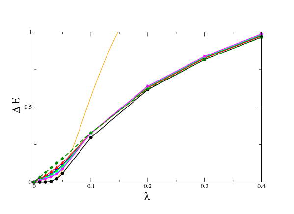
Figure 1: Data reported in Tables 1, 2 for $\Delta E$ as obtained in LPA, plotted as a function of the coupling $\lambda$. Lines joining the single points are included for convenience. $\Delta E_{exact}$ and $\Delta E_{WH}$ from Table 1 are respectively displayed as black circles with a continuous black line and green diamonds with a dashed green line. Then data from Table 2 are : blue squares, $\Delta E_{erg}$; red pointing up triangles, $\Delta E_{pt1}$; light green pointing left triangles, $\Delta E_{pt2}$; turquoise pointing down triangles, $\Delta E_{pt4}$; pink pointing right triangles, $\Delta E_{pt10}$, all joined by continuous lines of the respective colour. The continuous orange line joins the instanton data of Table 1.

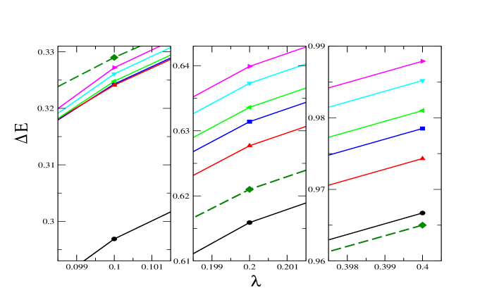
Figure 2: Details of Fig.1 at three values of the coupling, $\lambda=0.1,\,0.2$ and $0.4$. Coding is given in Fig.1.

From Fig. 1 it is evident that all computations in the LPA produce accurate results only above $\lambda=0.1$. In fact from the data in Table 2 we see that for $\lambda\geq 0.2$ the maximum distance of the various determinations from $\Delta E_{exact}$ is below $4\%$ but it reaches $10\%$ at $\lambda=0.1$.

In Fig. 2 it is shown that at $\lambda=0.4$ and $\lambda=0.2$, $\Delta E_{WH}$ is the closest estimate to $\Delta E_{exact}$, while at $\lambda=0.1$ it becomes the farthest. At the same time, the distance from $\Delta E_{exact}$ of the PT estimates at various $m$ grows with $m$, when $\lambda\geq 0.1$.

A totally different picture appears in Fig. 3 for $\lambda\leq 0.05$. In fact we observe that $\Delta E_{WH}$ approaches zero linearly with $\lambda$, then totally missing the exponential behavior of $\Delta E_{exact}$. On the other hand, the LPA PT determinations invert their order and in this region the determinations with lager $m$ show better agreement with $\Delta E_{exact}$. In addition they also show a slight change of concavity that improves for larger $m$.

In summary, while our findings show that the LPA calculations are altogether satisfactorily accurate for $\lambda\geq 0.1$, on the contrary they are quantitatively inadequate to reproduce $\Delta E_{exact}$ when $\lambda\leq 0.05$. In this case, some improvement is necessary.

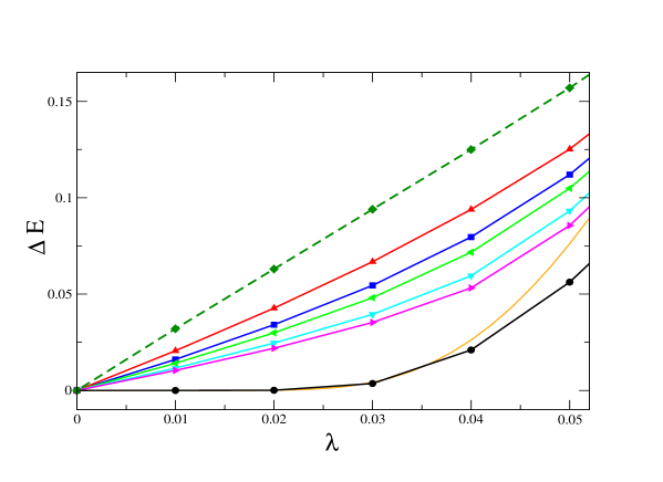
Figure 3: Details of Fig.1 at small values of the coupling $\lambda$. Coding is given in Fig.1.

III.3 Inclusion of the renormalization $Z_{k}$

In this section we finally present the gap $\Delta E$, corrected by the renormalization factor $Z_{k}$, i.e.

$$\Delta E=\sqrt{\frac{V_{k=0}(\varphi)^{\prime\prime}}{Z_{k=0}(\varphi)}}\;\;\Bigg{|}_{\varphi=0}$$ (32)

as obtained from the coupled flow equations for $V_{k}$ and $Z_{k}$. Table 3 contains the results of the NSA ERG flow and of the NSA PT flow for $m=1,2,3,4,10$, together with the corresponding value of the correction $Z_{k=0}(\varphi=0)$ displayed in parenthesis below. Again, the column with $\Delta E_{exact}$ is inserted for comparison.

$M^{2}=1$
$\;\;\lambda\;\;$	$\;\;\Delta E_{exact}\;\;$	$\;\;\Delta E_{erg}\;\;$	$\;\;\Delta E_{pt1}\;\;$	$\;\;\Delta E_{pt2}\;\;$	$\;\;\Delta E_{pt3}\;\;$	$\;\;\Delta E_{pt4}\;\;$	$\;\;\Delta E_{pt10}\;\;$
1	1.9341	1.9351	1.9344	1.9365	1.9384	1.9395	1.9417
		(1.0073)	(1.010)	(1.007)	(1.007)	(1.007)	(1.006)
0.02	1.0540	1.5043	1.0542	1.0542	1.0543	1.0543	1.0543
		(0.9993)	(1.0003)	(1.0003)	(1.0002)	(1.0002)	(1.0002)
$M^{2}=-1$
$\;\;\lambda\;\;$	$\;\;\Delta E_{exact}\;\;$	$\;\;\Delta E_{erg}\;\;$	$\;\;\Delta E_{pt1}\;\;$	$\;\;\Delta E_{pt2}\;\;$	$\;\;\Delta E_{pt3}\;\;$	$\;\;\Delta E_{pt4}\;\;$	$\;\;\Delta E_{pt10}\;\;$
0.4	0.9667	0.9764	0.9632	0.9688	0.9723	0.9743	0.9782
		(1.037)	(1.043)	(1.033)	(1.029)	(1.027)	(1.023)
0.3	0.8166	0.8276	0.8120	0.8182	0.8219	0.8239	0.8280
		(1.047)	(1.055)	(1.042)	(1.037)	(1.034)	(1.029)
0.2	0.6159	0.6300	0.6083	0.6162	0.6203	0.6227	0.6271
		(1.074)	(1.088)	(1.065)	(1.056)	(1.052)	(1.044)
0.1	0.2969	0.3158	0.2702	0.2888	0.2950	0.2980	0.3037
		(1.264)	(1.356)	(1.225)	(1.188)	(1.170)	(1.140)
0.05	0.0562	X	X	0.0168	0.0262	0.0293	0.0333
				(7.503)	(4.318)	(3.648)	(2.852)

Table 3: $\Delta E$ for various couplings $\lambda$ and for $M^{2}=1$ or $M^{2}=-1$, as obtained from the Schroedinger equation ($\Delta E_{exact}$) and from the coupled flow equation for $V_{k}$ and $Z_{k}$, respectively in the NSA ERG case ($\Delta E_{erg}$), and the NSA PT case with $m=1,2,3,4,10$ ($\Delta E_{pt1-pt10}$). The correction $Z_{k}(\varphi=0)$ is reported in parenthesis.

The NSA PT determinations of $\Delta E$ when $M^{2}=1$ strongly improve the agreement obtained with the LPA calculation. In fact, from Table 3 we observe that at $\lambda=1$ the error for the worse determination ($\Delta E_{pt10}$) is about $0.4\%$, but decreases to $0.02\%$ for $\Delta E_{pt1}$; at $\lambda=0.02$ the error is always around $0.03\%$. In addition, for both values of $\lambda$, we find $\Delta E_{pt1}\leq\Delta E_{erg}\leq\Delta E_{pt3}$ as in the LPA case. In all determinations, the correction factor $Z_{k=0}$ is extremely small.

By switching to the case $M^{2}=-1$, for the PT case we find $\Delta E_{pt1}<\Delta E_{exact}<\Delta E_{pt10}$ for $\lambda>0.1$, with an interval $(\Delta E_{pt10}-\Delta E_{pt1})/\Delta E_{pt10}$ of order $2\%\div 3\%$ if $\lambda>0.2$, and around $10\%$ at $\lambda=0.1$. Instead, at $\lambda=0.05$, we observe a rather different picture, because in the $m=1$ case an imaginary component of the potential is generated and no clear convergence is observed whereas, at larger $m$, a definite value of $\Delta E$ together with very large $Z_{k=0}>>1$ is obtained but these estimates substantially differ from $\Delta E_{exact}$.

For the NSA ERG data, we observe an unusual picture: in fact $\Delta E_{erg}$ is no longer similar to $\Delta E_{pt1}$ but it is rather closer to $\Delta E_{pt10}$ and, below $\lambda=0.3$, it becomes even bigger: $\Delta E_{erg}>\Delta E_{pt10}$. At $\lambda=0.05$, we do not find convergence to a definite value for $\Delta E_{erg}$, much in the same way as it is observed for $\Delta E_{pt1}$.

Finally, at smaller $\lambda$, no convergence is found, neither for the NSA PT case at any $m$, nor for the NSA ERG and we conclude that if $M^{2}=1$ the NSA determinations of the gap improve the LPA results, but if $M^{2}=-1$, this is true only in the perturbative region ($\lambda>0.1$ and $Z_{k=0}\sim 1$). At smaller $\lambda$ when the non-perturbative tunnelling effects become relevant, computations become impracticable.

Now we turn to the SA flow and show the output obtained in the ERG case, i.e. from the flow equations (21), (II.1), that include non-linear effects in the ’time’ derivatives, due to the presence of $\eta_{k}$. Unfortunately, these non-linear terms substantially affect the numerical convergence of the PDE, and we can trust the results of this scheme only for $\lambda\geq 0.08$. In order to get some insight, we report in Fig. 4 the relative error on the determinations $\delta=(\Delta E_{erg}-\Delta E_{exact})/\Delta E_{exact}$ as a function of the coupling $\lambda\geq 0.08$, for the SA ERG (blue upper positive curve).

The determination of $\delta$ for the NSA ERG (green negative curve) is also included for comparison. We observe that the relative error becomes larger for smaller values of the coupling in both cases, but $\delta$ of the SA ERG is about twice the one of the NSA ERG at $\lambda=0.08$. We also performed the analysis of the SA PT flow corresponding to the ’B-scheme’ of Bonanno et al. (2020) but we do not report the corresponding curve, as it essentially produces even worse results than those of the SA ERG scheme, shown by the blue curve in Fig. 4.

Instead, the computation of the simplified SA ERG flow, where the nonlinear effects in Eqs. (21) and (II.1) are discarded by taking $\eta_{k}=0$, turns out to be much stabler than the full SA (ERG and PT) flows. This is evident from the plot of the corresponding $\delta$ (red lower positive curve) in Fig. 4, which is of the same size (although opposite in sign) of the NSA ERG relative error.

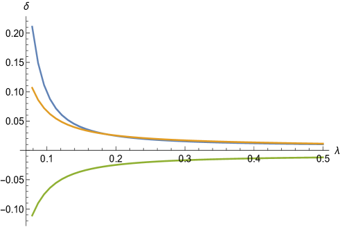
Figure 4: Relative error $\delta=(\Delta E_{erg}-\Delta E_{exact})/\Delta E_{exact}$ for the SA ERG (blue upper positive curve), and for the simplified SA ERG with $\eta_{k}=0$ (orange lower positive curve), and for the NSA ERG (green negative curve), vs. the coupling $\lambda$.

On the PT side, the flow that can consistently be compared with the SA ERG flow with $\eta_{k}=0$, corresponds to the ’simplified type-C scheme’ of Bonanno et al. (2020), reported in Eqs. (27), (28). In fact, we integrated these two SA simplified flows and, in addition to a small relative error, we also found in both cases convergence at smaller values of the coupling, so that our analysis could be pushed down to $\lambda=0.03$. Therefore, below, we discuss in more detail the output of these two sets of PDE, namely Eqs. (21), (II.1) and (27), (28), as representative respectively of the ERG SA and PT SA flow, and the relative data are reported in Table 4 and also collectively shown in Fig.5.

$M^{2}=1$
$\;\;\lambda\;\;$	$\;\;\Delta E_{exact}\;\;$	$\;\;\Delta E_{erg}\;\;$	$\;\;\Delta E_{pt1}\;\;$	$\;\;\Delta E_{pt2}\;\;$	$\;\;\Delta E_{pt3}\;\;$	$\;\;\Delta E_{pt4}\;\;$	$\;\;\Delta E_{pt10}\;\;$
1	1.9341	1.9249	1.9197	1.9279	1.9311	1.9329	1.9362
		(1.009)	(1.010)	(1.008)	(1.007)	(1.007)	(1.006)
0.02	1.0540	1.0539	1.0538	1.0540	1.0541	1.0543	1.0542
		(1.003)	(1.0003)	(1.0003)	(1.0002)	(1.0002)	(1.0002)
$M^{2}=-1$
$\;\;\lambda\;\;$	$\;\;\Delta E_{exact}\;\;$	$\;\;\Delta E_{erg}\;\;$	$\;\;\Delta E_{pt1}\;\;$	$\;\;\Delta E_{pt2}\;\;$	$\;\;\Delta E_{pt3}\;\;$	$\;\;\Delta E_{pt4}\;\;$	$\;\;\Delta E_{pt10}\;\;$
0.4	0.9667	0.9514	0.9427	0.9564	0.9617	0.9645	0.9699
		(1.040)	(1.048)	(1.035)	(1.031)	(1.029)	(1.024)
0.3	0.8166	0.8011	0.7922	0.8062	0.8116	0.8144	0.8200
		(1.051)	(1.062)	(1.045)	(1.039)	(1.036)	(1.031)
0.2	0.6159	0.5994	0.5899	0.6049	0.6105	0.6136	0.6192
		(1.082)	(1.101)	(1.071)	(1.061)	(1.056)	(1.047)
0.1	0.2969	0.2769	0.2660	0.2844	0.2905	0.2935	0.2994
		(1.308)	(1.400)	(1.245)	(1.204)	(1.185)	(1.151)
0.05	0.0562	0.0334	0.0306	0.0483	0.0516	0.0527	0.0539
		(5.872)	(7.328)	(3.291)	(2.763)	(2.559)	(2.255)
0.04	0.0210	0.0013	0.0027	0.0141	0.0167	0.0178	0.0224
		(138.2)	(80.51)	(8.649)	(6.252)	(5.397)	(3.162)
0.03	0.0036	X	0.0016	0.0015	0.0036	0.0059	0.0099
			(90.71)	(14.67)	(11.27)	(6.51)	(3.85)

Table 4: Same as in Table 3, but with $\Delta E$ derived from the SA ERG flow in Eqs. (21), (II.1) and SA PT flow in Eqs. (27), (28).

A comparison of Fig.5 and Fig.1 clearly indicates that the agreement of the SA data with $\Delta E_{exact}$ is improved with respect to the LPA data in the region of small $\lambda$. In addition, from Table 4 we find $\Delta E_{pt1}<\Delta E_{erg}<\Delta E_{pt2}$, with the exception of the smallest values of the coupling $\lambda=0.04$ and $\lambda=0.03$, which we shall comment on later. In both rows with $M^{2}=1$ in Table 4, we find $\Delta E_{pt1}<\Delta E_{exact}<\Delta E_{pt10}$, but it must be remarked that the difference $\Delta E_{pt10}-\Delta E_{pt1}$, although smaller than $1\%$ in the two cases, is twice the corresponding difference for the NSA case.

Turning to the $M^{2}=-1$ problem, a picture of the data obtained at $\lambda=0.4,\,0.2,\,0.1$ is given in the three panels of Fig.6 where, together with $\Delta E_{exact}$ (black circles), the SA determination of $\Delta E_{pt1}$ (red triangles pointing up) and of $\Delta E_{pt10}$ (pink triangles pointing right) and, in addition, also the NSA determination of $\Delta E_{pt1}$ (red stars) and of $\Delta E_{pt10}$ (pink crosses) are displayed. In all panels the point $\Delta E_{exact}$ is always between the $\Delta E_{pt10}$ and $\Delta E_{pt1}$ and the distance between these two determinations is smaller for the NSA case at $\lambda=0.4$ but it becomes practically equal to the one for the SA case at $\lambda=0.1$ At smaller coupling $\lambda$, as already seen, the NSA flow fails to converge and only the SA determinations are available at very low $\lambda$.

Finally, the region of $\lambda\leq 0.05$ is displayed in Fig.7 where the SA determinations are plotted together with $\Delta E_{exact}$ and $\Delta E_{inst}$. Fig.7 clearly shows the importance of the inclusion of $Z_{k=0}$ (which has now values of order 10 or in some cases even 100) : points that in the LPA approximation are very far from $\Delta E_{exact}$, now have substantially reduced their distance.

In particular, even the worst determination ($\Delta E_{pt1}$) at $\lambda=0.05$ shows an agreement( about $35\%$) very similar to that of the instanton calculation. At $\lambda=0.04$, while $\Delta E_{pt1}$ and $\Delta E_{erg}$ become very small, calculations at larger $m$ (e.g. $m=10$) are reasonably accurate, with error below $10\%$.

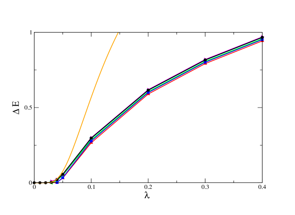
Figure 5: Data reported in Table 4 for $\Delta E$, as obtained by including the correction $Z_{k}$ in the simplified SA scheme, plotted vs. $\lambda$. Again, for convenience, lines joining the points are included. Also the same coding as in Fig. 1 is adopted, with the exception of $\Delta E_{WH}$ data, not included here as no $Z_{k}$ correction is available.

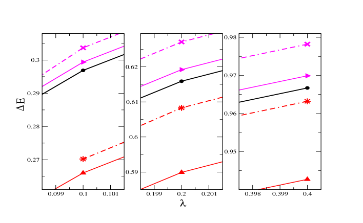
Figure 6: Details of $\Delta E$, including the correction $Z_{k}$, at three values of the coupling $\lambda=0.1,\,0.2\,0.4$. In addition to $\Delta E_{exact}$ data from Table 1 (black circles with a continuous black line), we plot $\Delta E_{pt1}$ and $\Delta E_{pt10}$ from Table 3 for the NSA case, respectively with red stars and pink crosses, both with dot-dashed lines of the respective colour attached. Moreover, $\Delta E_{pt1}$ and $\Delta E_{pt10}$ from Table 4 for the SA case, are plotted with the same coding as in Figs.1 and 5, i.e. the former with red triangles pointing up and the latter with pink triangles pointing right. Both have continuous lines of the respective colour attached.

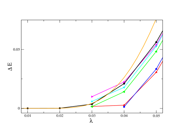
Figure 7: Details at small values of $\lambda$ of Fig.5. $\Delta E$, including the correction $Z_{k}$, is plotted vs. $\lambda$. Coding is the same as in Figs.1, 5 and 6.

At $\lambda=0.03$, $\Delta E_{inst}$ still differs from $\Delta E_{exact}$ of about $30\%$, while the PT determinations at $m=1$ and $m=2$ are off of $45\%$. The case with $m=3$ (not reported in Fig.7 - see Table 4) practically reproduces $\Delta E_{exact}$, and $m=10$ yields too large values of the gap. Instead, the ERG flow fails to converge at $\lambda=0.03$, and this is probably due to an increasing $Z_{k}$ as $k\to 0$ (already at $\lambda=0.04$ we find $Z_{k=0}=138$) that reduces the gap to such a small value to be comparable with the numerical precision.

The same kind of problem is observed at $\lambda=0.02$ not only for the ERG flow, but also for the PT flow with $m=1$ and $m=2$. Yet, at $m=3,4,10$ we find convergence, respectively to $3\;10^{-4}$, $9\;10^{-4}$, $3.4\;10^{-3}$ which, at least for $m=3$, is of the same order of magnitude of $\Delta E_{exact}$; however we prefer not to report these values in Table 4 because, especially for the first two cases, they are comparable with the numerical precision of our computation.

Therefore, we conclude that, when including the correction $Z_{k=0}$, our computation qualitatively reproduces the exponential trend induced by the tunnelling in the region $\lambda=0.03-0.05$.

IV Conclusions

The computation of the energy gap in the quanto-mechanical double well potential by means of the derivative expansion of the Functional Renormalization Group flow equations performed in this paper, essentially aims at understanding to which extent this approach can quantitatively keep under control the simplest one-dimensional non-perturbative effect, associated to the tunneling between the two vacua. Therefore, we mainly focus on the comparison of the average estimates of various formulations of the flow equations with the accurate results coming from the Schroedinger equation resolution of the problem.

The improvement associated to the inclusion of higher terms of the derivative expansion is evident even in the case of the anharmonic oscillator with $M^{2}=1$, as shown in Tables 2, 3, 4. In this case, the agreement of our estimates is always excellent (with a relative error that never exceeds $1\%$), but the improvement when going from the LPA in Table 2 to the the NSA approximation in Table 3 and simplified SA in Table 4, is evident especially in the large coupling case $\lambda=1$.

Turning to the double well case with $M^{2}=-1$, we can clearly distinguish different regimes associated to the explored range $\lambda$. Fig. 1 shows that the estimates obtained in LPA for $\lambda\geq 0.2$ are globally accurate; then , for lower $\lambda$ the agreement diminishes and for $\lambda\geq 0.05$, this approximation hardly reproduces the exponential approach to zero of $\Delta E$. As shown in Fig. 3, the WH approach has an inaccurate linear behavior, while for instance the PT potential with $m=10$ shows a qualitative agreement with the exact values.

Then, the inclusion of $Z_{k}$ in the simplified SA version of the flow equations, clearly brings a strong improvement in the region $0.1\leq\lambda\leq 0.03$ as seen in Figs. 5 and 7. Even at $\lambda=0.04$, some estimates turn out to be more accurate than the instanton determination of $\Delta E$, which is then no longer valid at $\lambda=0.03$ where $\Delta E_{inst}$ becomes the most precise estimate displayed. However, it must be remarked that already at $\lambda=0.04$, and more evidently at smaller $\lambda$, not all formulations of the flow equations show clear convergence within our numerical precision. This drawback becomes too strong at $\lambda=0.02$ and we do not trust our findings at this value of the coupling.

To summarize, the inclusion of the first correction to the LPA represents a strong improvement in the range $0.1\leq\lambda\leq 0.03$, indicating that the derivative expansion of the RG flow does actually reproduce the non-perturbative exponential decay of $\Delta E$. It is conceivable to expect that the next step in the derivative expansion, corresponding to to inclusion of four derivatives in the original action, could further enhance the convergence of the PDE for $\lambda\leq 0.03$.

A final comment is dedicated to the different approaches adopted in our analysis. We found that, both NSA and SA (in either full or simplified version) are equally accurate as long as the wave function renormalization $Z_{k}\sim 1$, as shown in Fig. 4. But, as soon as $Z_{k}$ grows up to non perturbative values, the NSA and the full SA schemes become not trustable or do not converge, the former because of the incomplete cancellation of the term $Z_{k}p^{2}$ in the propagators, and the latter because of the presence of non-linear terms in the ’time’ derivative of $Z_{k}$, included in $\eta_{k}$. In both cases the growth of $Z_{k}$ has these undesired effects. Still, in the simplified SA approach, where these problems are circumvented, PDE are integrated at much lower values of $\lambda$ and, at least in the PT flow with $m$ suitably optimized, providing precise estimates of $\Delta E$.