Conservative Hamiltonian Monte Carlo

Abstract

We introduce a new class of Hamiltonian Monte Carlo (HMC) algorithm called Conservative Hamiltonian Monte Carlo (CHMC), where energy-preserving integrators, derived from the Discrete Multiplier Method, are used instead of symplectic integrators. Due to the volume being no longer preserved under such a proposal map, a correction involving the determinant of the Jacobian of the proposal map is introduced within the acceptance probability of HMC. For a $p$-th order accurate energy-preserving integrator using a time step size $\tau$, we show that CHMC satisfies stationarity without detailed balance. Moreover, we show that CHMC satisfies approximate stationarity with an error of $\mathcal{O}(\tau^{(m+1)p})$ if the determinant of the Jacobian is truncated to its first $m+1$ terms of its Taylor polynomial in $\tau^{p}$. We also establish a lower bound on the acceptance probability of CHMC which depends only on the desired tolerance $\delta$ for the energy error and approximate determinant. In particular, a cost-effective and gradient-free version of CHMC is obtained by approximating the determinant of the Jacobian as unity, leading to an $\mathcal{O}(\tau^{p})$ error to the stationary distribution and a lower bound on the acceptance probability depending only on $\delta$. Furthermore, numerical experiments show increased performance in acceptance probability and convergence to the stationary distribution for the Gradient-free CHMC over HMC in high dimensional problems.

60J22, 65C05, 65C40, 65P10

1 Introduction

Since its inception in the mid-twentieth century, Markov chain Monte Carlo (MCMC) algorithms have been widely used in statistical physics to estimate various physical observable quantities [31, 22, 14]. Moreover, in the past few decades, MCMC methods have gained wide spread adoption in parameter estimation and Bayesian statistics [16, 38, 17]. More recently, MCMC algorithms have also found applications in machine learning, such as in Bayesian Learning and Bayesian Neural Networks [33, 1, 12, 27].

In essence, MCMC algorithms enables the generation of a sequence of samples drawn from complex distributions. Such samples are drawn in a computational feasible way relying only on information from previous successive samples in the sequence, satisfying the Markov property. Under appropriate conditions, this sequence converges to some limiting distribution that corresponds to a distribution of interest, usually called the target distribution. To obtain statistical information on the target distribution, a sufficiently large finite set of samples is drawn in order to overcome correlation between successive samples. With such a finite set of samples, various statistical quantity of interest can then be estimated via Monte Carlo integration.

More precisely, for a given target distribution $\pi:\mathbb{R}^{d}\rightarrow\mathbb{R}$, Markov Chain Monte Carlo algorithms (MCMC) generate a sequence of samples drawn identically from a Harris ergodic Markov chain $X=\{X_{i}\}_{i=0}^{\infty}$ in $\mathbb{R}^{d}$ with a stationary distribution $\pi$ [26]. For a statistical quantity of interest $f:\mathbb{R}^{d}\rightarrow\mathbb{R}$ with a finite variance on the random variable $f(X)$, the Markov Chain central limit theorem [26] guarantees that

(1) $$\frac{\sqrt{N}}{\sigma}\left(\frac{1}{N}\sum\limits_{i=1}^{N}f(X_{i})-\int\limits_{\mathbb{R}^{d}}\pi(x)f(x)\text{d}x\right)\xrightarrow{\mathcal{D}}\mathcal{N}(0,1),$$

where convergence is in distribution and $\displaystyle\sigma^{2}=\text{var}(f(X_{0}))+2\sum_{i=1}^{\infty}\text{cov}(f(X_{0}),f(X_{i})).$ In other words, with a probability close to 1, the empirical average $\displaystyle\frac{1}{N}\sum\limits_{i=1}^{N}f(X_{i})$ converges to $\displaystyle\int\limits_{\mathbb{R}^{d}}\pi(x)f(x)\text{d}x$ at a rate $\mathcal{O}(N^{-\frac{1}{2}})$. Due to the Markovian nature of the successive samples, the initial samples are highly correlated and are discarded in practice after a warm-up period has set in. Various diagnostics and metrics are used to determine this warm-up period and access convergence of the Markov chain in practice [8, 17].

MCMC algorithms draw each sample of the Markov Chain through a proposal process followed by an acceptance criteria. MCMC methods, such as Metropolis-Hastings (MH) [31, 22], Gibbs sampling [18, 10], Metropolis-Adjusted Langevin Algorithm (MALA) [37, 36], Hybrid Monte Carlo or Hamiltonian Monte Carlo (HMC) [14, 32, 34, 5, 7], have their own proposal processes and acceptance criteria designed to ensure that $\pi$ is the stationary distribution of the resulting Markov Chain $\{X_{i}\}_{i=0}^{N}$. With stationarity established, expectations of the target distribution $\pi$ can be estimated by empirical average in (1) with high probability.

One of the most widely used MCMC algorithms is the MH algorithm, also known as random walk MCMC. In MH, a new proposed sample is obtained by drawing from a normal distribution, or another distribution which can be efficiently sampled from, centred about a previous sample drawn from the Markov Chain. The acceptance probability is chosen to favor samples towards high density regions of the target distribution $\pi$, while ensuring $\pi$ remains as the stationary distribution of the Markov Chain. While MH has a simple implementation, it suffers from low acceptance probability in high dimensions [5]. Furthermore, accepted proposals are generally drawn near the previous sample, slowing the exploration of the high density regions of $\pi$. Thus, more sophisticated MCMC methods, such as MALA and HMC, were introduced to improve the sampling of high density regions, especially in high dimensions. In this paper, we further improve upon HMC’s sampling efficacy by utilizing energy-preserving methods, leading to a new MCMC algorithm called Conservative Hamiltonian Monte Carlo (CHMC).

This paper is organized as follows. In Section 1.1, we give a brief review of HMC and relevant details to CHMC. In Section 1.2, we give an overview of various conservative integrators known in the geometric numerical integration literature and motivate why we employed the Discrete Multiplier Method. In Section 2, we introduce the CHMC algorithm and show various lemmas leading to our main result of Theorem 2.5 and its Corollary 2.7 on error estimates for the stationarity of CHMC using approximate determinants. In Section 3, we discuss practical considerations of CHMC, leading to the Gradient-free CHMC method. Section 4.1 showcases numerical results comparing the different variants of CHMC versus HMC, as well as improvement on acceptance probability and in convergence with Gradient-free CHMC over HMC for high dimensional problems. Finally, we give some concluding remarks in Section 5.

1.1 Brief overview on HMC

Before we introduce CHMC, we give a brief overview of HMC and emphasize the aspects related to CHMC. We also introduce some common notations that will be used throughout this paper. This section can be skipped for readers who are already familiar with HMC. For a more thorough introduction of HMC, we recommend [34, 5, 7].

As detailed in [5], traditional random walk MCMC is less effective at estimating from a high dimensional target distribution $\pi$ because proposals are drawn randomly, without incorporating explicit information about the high density regions of $\pi$. As the dimension of $\pi$ increases, such proposed samples are less likely to be drawn in directions leading toward these high density regions. In contrast, HMC adds directional information by extending the sample space to include momentum variables, leading to proposed samples which favour more towards, and stay near, high density regions of $\pi$. Additionally, HMC can maintain a higher acceptance probability than MH for proposed samples separated in large distances, by leveraging key characteristics of Hamiltonian dynamical systems.

More precisely, for a target distribution $\pi:\mathbb{R}^{d}\rightarrow\mathbb{R}$ with variables ${\boldsymbol{q}}\in\mathbb{R}^{d}$, the standard HMC algorithm extends the sample space of $\pi$ to $\mathbb{R}^{2d}$ by introducing momentum variables ${\boldsymbol{p}}\in\mathbb{R}^{d}$ with a normal distribution $\mathcal{N}({\boldsymbol{0}},M)$, where $M$ is a constant $d\times d$ positive definite symmetric matrix. The resulting joint distribution of the extended sample space satisfies

(2) $$\pi({\boldsymbol{q}},{\boldsymbol{p}}) \propto e^{-H({\boldsymbol{q}},{\boldsymbol{p}})},~{}~{}\text{where}$$

(3) $$H({\boldsymbol{q}},{\boldsymbol{p}}) =U({\boldsymbol{q}})+K({\boldsymbol{p}}),$$

is the Hamiltonian function, with $U({\boldsymbol{q}})=-\log\pi({\boldsymbol{q}})$ as the potential energy function and $K({\boldsymbol{p}})=\frac{1}{2}{\boldsymbol{p}}^{T}M^{-1}{\boldsymbol{p}}$ as the kinetic energy function.

The HMC algorithm begins by randomly drawing ${\boldsymbol{q}}^{0}$ and ${\boldsymbol{p}}^{0}\sim\mathcal{N}({\boldsymbol{0}},M)$, then a proposal for a new sample $({\boldsymbol{q}}^{*},{\boldsymbol{p}}^{*})$ is obtained by numerically solving the Hamiltonian equations starting at $({\boldsymbol{q}}^{0},{\boldsymbol{p}}^{0})$,

(4) $$\begin{split}\frac{d}{dt}{\boldsymbol{q}}(t)&=\frac{\partial}{\partial{\boldsymbol{p}}}H({\boldsymbol{q}}(t),{\boldsymbol{p}}(t))=M^{-1}{\boldsymbol{p}}(t),\\ \frac{d}{dt}{\boldsymbol{p}}(t)&=-\frac{\partial}{\partial{\boldsymbol{q}}}H({\boldsymbol{q}}(t),{\boldsymbol{p}}(t))=-\frac{\partial U}{\partial{\boldsymbol{q}}}({\boldsymbol{q}}(t)),\end{split}$$

for some prescribed length of time, $T$.

There are two main properties of the Hamiltonian system (4) that HMC relies on. By differentiating $H({\boldsymbol{q}}(t),{\boldsymbol{p}}(t))$ with respect to time, the Hamiltonian function $H$ is conserved on any solution $({\boldsymbol{q}}(t),{\boldsymbol{p}}(t))$ of (4). That is, for any choice of $T$, $H({\boldsymbol{q}}(t+T),{\boldsymbol{p}}(t+T))=H({\boldsymbol{q}}(t),{\boldsymbol{p}}(t))$. This first property enables HMC to obtain samples that are separated by large distances, as discussed below. Moreover, viewing the solution of (4) as the map $\varphi_{T}:\mathbb{R}^{2d}\rightarrow\mathbb{R}^{2d}$ defined by $\varphi_{T}({\boldsymbol{q}}^{0},{\boldsymbol{p}}^{0})=({\boldsymbol{q}}(T),{\boldsymbol{p}}(T))$, it can be shown that $\varphi_{T}$ is a volume-preserving map, which means the determinant of the Jacobian of $\varphi_{T}$ with respect to $({\boldsymbol{q}}^{0},{\boldsymbol{p}}^{0})$ satisfies $\det J_{\varphi_{T}}=1$. This second property enables the acceptance probability of HMC to be simplified, as we shall see shortly.

Starting from an initial sample ${\boldsymbol{q}}^{0}={\boldsymbol{\theta}}^{0}$, a sample of the momentum variable ${\boldsymbol{p}}^{0}$ is drawn from a normal distribution $\mathcal{N}({\boldsymbol{0}},M)$ and a new sample $({\boldsymbol{q}}^{*},{\boldsymbol{p}}^{*})$ is proposed by numerically solving the Hamiltonian system (4) using a symplectic method, denoted by the proposal map $\Psi_{SYM}$. A symplectic method preserves the symplectic structure of the map $\Psi_{SYM}$ and is thus volume preserving [21]. Using the same acceptance probability $\alpha$ as the symmetric proposal of the MH algorithm, the following HMC algorithm generates a sequence $\{{\boldsymbol{\theta}}^{i}\}_{i=0}^{\infty}$ that satisfies stationarity [34] using detailed balance.

1 Pick ${\boldsymbol{\theta}}^{0}$

2 for $i=0,1,2,\dots$ do

3       ${\boldsymbol{q}}^{0}\leftarrow{\boldsymbol{\theta}}^{i}$

4       Draw ${\boldsymbol{p}}^{0}\sim\mathcal{N}({\boldsymbol{0}},M)$

5       $({\boldsymbol{q}}^{*},{\boldsymbol{p}}^{*})\leftarrow\Psi_{SYM}({\boldsymbol{q}}^{0},{\boldsymbol{p}}^{0};H,\tau,N)$

6       $\alpha\leftarrow\min\left\{1,\exp\left(-\left[H({\boldsymbol{q}}^{*},{\boldsymbol{p}}^{*})-H({\boldsymbol{q}}^{0},{\boldsymbol{p}}^{0})\right]\right)\right\}$

7       ${\boldsymbol{\theta}}^{i+1}\leftarrow\begin{cases}&{\boldsymbol{q}}^{*}\text{ with probability }\alpha\\ &{\boldsymbol{\theta}}^{i},\text{ with probability }1-\alpha\end{cases}$

Pseudocode 1 HMC Algorithm

To solve (4) numerically, the Leapfrog scheme or Velocity Verlet method is typically used. The Leapfrog scheme is a second-order explicit symplectic method [21] and other higher-order explicit symplectic methods have also been introduced for HMC in [6]. More explicitly, for a fixed number of time steps $N$, and time step size $\tau=\frac{T}{N}$, the Leapfrog scheme yields the numerical solution $({\boldsymbol{q}}^{i+1},{\boldsymbol{p}}^{i+1})$, which denotes the numerical solution at the $(i+1)$-st time step, using the explicit update formula

(5) $$\begin{split}{\boldsymbol{p}}^{i+\frac{1}{2}}&={\boldsymbol{p}}^{i}-\frac{\tau}{2}\frac{\partial U}{\partial{\boldsymbol{q}}}({\boldsymbol{q}}^{i}),\\ {\boldsymbol{q}}^{i+1}&={\boldsymbol{q}}^{i}+\tau M^{-1}{\boldsymbol{p}}^{i+\frac{1}{2}},\\ {\boldsymbol{p}}^{i+1}&={\boldsymbol{p}}^{i+\frac{1}{2}}-\frac{\tau}{2}\frac{\partial U}{\partial{\boldsymbol{q}}}({\boldsymbol{q}}^{i+1}).\end{split}$$

Similar to the map $\varphi_{T}$, we can view taking one time step of the Leapfrog scheme as the map $\Psi_{LF}:\mathbb{R}^{2d}\rightarrow\mathbb{R}^{2d}$ defined by $\Psi_{LF}({\boldsymbol{q}}^{i},{\boldsymbol{p}}^{i})=({\boldsymbol{q}}^{i+1},{\boldsymbol{p}}^{i+1})$ using (5). Moreover, the map $\Psi_{LF}$ is symplectic and so volume-preserving [21], which implies the determinant of the Jacobian of $\Psi_{LF}$ with respect to $({\boldsymbol{q}}^{i},{\boldsymbol{p}}^{i})$ satisfies $\det J_{\Psi_{LF}}=1$. Thus, after taking $N$ time steps using the Leapfrog scheme starting from $({\boldsymbol{q}}^{0},{\boldsymbol{p}}^{0})$, $({\boldsymbol{q}}^{N},{\boldsymbol{p}}^{N})$ approximates $({\boldsymbol{q}}(T),{\boldsymbol{p}}(T))$. Hence, the proposal map in Algorithm 1 is $\Psi_{SYM}=\Psi^{N}_{LF}$, which denotes the $N$-times composition of the Leapfrog scheme (5).

As discussed previously, HMC is able to maintain a high acceptance probability for proposals which may be a great distance from their initial point, $({\boldsymbol{q}}^{0},{\boldsymbol{p}}^{0})$. Specifically, using a backward error analysis of the Leapfrog method, it can be shown that [21, 4]

(6) $$H({\boldsymbol{q}}^{N},{\boldsymbol{p}}^{N})-H({\boldsymbol{q}}^{0},{\boldsymbol{p}}^{0})=\mathcal{O}(\tau^{2}),$$

leading to a high acceptance probability $\alpha$ for HMC for small enough $\tau$. Furthermore, improvements can be made to Algorithm 1 to tune the other parameters $\tau,T$ and the mass matrix $M$, such as No-U-Turn sampling [24], tuning step size [4] and generalizing $M$ to depend on ${\boldsymbol{q}}$ in Riemannian HMC [19, 5].

Despite the many advantages of HMC, there remains aspects of the algorithm which may still be improved. By (6), the Leapfrog scheme (5) does not conserve the Hamiltonian exactly. As the acceptance probability of HMC depends on the error in the Hamiltonian, this can lead to a decrease in accepted proposals as the dimension $d$ increases. Indeed, as shown in [4] with suitable regularity assumptions on $U$, the time step size $\tau$ must scale as $\mathcal{O}(d^{-\frac{1}{4}})$ in order to maintain a constant acceptance probability as $d$ increases. Another aspect of HMC which can limit its applicability is the requirement of computing gradients of the target distribution $\pi$ through the term $\dfrac{\partial U}{\partial{\boldsymbol{q}}}$ introduced in (5). As discussed in [13], requiring gradients of $\pi$ may prohibit HMC from certain applications due to steep computational costs in high dimensional setting. Furthermore, in Bayesian applications, such as Pseudo-Marginal MCMC [2] and Approximate Bayesian Computation MCMC [29], the target posterior distribution does not have analytical expressions and can only be estimated, making HMC not directly applicable in these cases. These potential areas for improvement of HMC motivated us to pursue our present work on CHMC.

The main goal of CHMC is to leverage recent advance in exactly energy-preserving numerical scheme, in place of the Leapfrog scheme or other symplectic schemes, to improve on acceptance probability as the dimensionality of the target distribution increases. There are several types of energy-preserving schemes, such as average vector field method [35], projection method [21], discrete gradient method [25, 30] and Discrete Multiplier Method (DMM) [39]. We will use a specific DMM scheme to numerically solve the Hamiltonian system (4) while preserving the Hamiltonian up to machine precision. One main advantage of DMM over the other conservative methods above is that DMM inherently leads to gradient-free schemes that satisfy several key properties to be discussed. It is important to note that such energy-preserving schemes are generally not volume-preserving. Thus, in order for stationarity to hold for the resulting Markov chain, an additional term involving the determinant of the Jacobian of the proposal map must be included in the acceptance probability $\alpha$ of the CHMC algorithm. Thus, the main goal of this work is to investigate the potential advantages obtained by employing a gradient-free, energy-preserving DMM scheme in place of the volume-preserving symplectic schemes typically utilized in HMC. Before we begin our discussion of CHMC, we present a brief overview of energy-preserving schemes and the Discrete Multiplier Method.

1.2 Motivation on Discrete Multiplier Method

In general, a dynamical system is a first-order system of ordinary differential equations, like the Hamiltonian system (4), that can have multiple conserved quantities, which are functions that remain constant as the system evolves. Typically, such quantities include energy and momentum but nontrivial time-dependent conserved quantities can exist also for dissipative systems [39]. Conservative numerical schemes approximate the solutions of dynamical systems while preserving the conserved quantities across each time step and they are well-studied in the field of geometric numerical integration. In general, similar to symplectic methods, conservative numerical methods can have favorable long-term stability properties [41] over traditional numerical methods.

Specific to Hamiltonian systems and HMC, conservative numerical schemes that preserve the Hamiltonian are energy-preserving (EP) schemes. There are several classes of EP schemes known within the literature of geometric numerical integration. We discuss briefly several prominent schemes and reasons why we did not utilized them over DMM for CHMC. First, specialized Runge-Kutta methods in [11] have been constructed to preserve Hamiltonian of a polynomial form. However, for general Hamiltonians and hence general target distributions, no Runge-Kutta method can preserve all polynomials due to a barrier theorem by [28]. On the other hand, the average vector field method (AVF) [35] is an energy-preserving scheme that applies to general Hamiltonian functions. However, deriving an AVF scheme involves analytical integration or numerical quadrature of gradients of the Hamiltonian, making this approach potentially expensive for high dimensional applications of HMC. Another general class of conservative schemes is the projection method, where a traditional integrator is employed first, then the numerical solution is subsequently projected onto the level set of the Hamiltonian function. However, projection methods can suffer from instability when there are bounded components of the level set nearby unbounded ones [41]. Moreover, projection methods do not satisfy the reversibility criteria needed for stationary of HMC. Finally, another general class of conservative schemes is the discrete gradient method [30] which can preserve multiple conserved quantities using a skew-symmetric tensor representation of the right hand side of the dynamical system. Specific to Hamiltonian systems, the Itoh–Abe discrete gradient method [25] bears similarities to the DMM scheme that we will employ for CHMC. In particular, we utilize a symmetrized version of the Itoh–Abe discrete gradient scheme in order to satisfy reversibility for HMC.

The Discrete Multiplier Method was introduced in [39] as a class of general conservative integrators for dynamical systems that can preserve multiple conserved quantities of arbitrary forms up to machine precision. The main idea is to discretize the so-called conservation law multipliers associated with conserved quantities so that discrete chain rules and other compatibility conditions are satisfied. Such conservative integrators have since been applied to a wide-variety of problems within the mathematical sciences, including many-body systems [40], vortex-blob models [20] and piecewise smooth systems [23]. For the purpose of deriving energy-preserving schemes for CHMC, we employ a symmetrized version of DMM scheme introduced in the next section.

2 Theoretical results of Conservative Hamiltonian Monte Carlo

In this section, we propose an extension of HMC to obtain samples from the joint density $\displaystyle\pi({\boldsymbol{q}},{\boldsymbol{p}})=e^{-H({\boldsymbol{q}},{\boldsymbol{p}})}$, where $H({\boldsymbol{q}},{\boldsymbol{p}})$ is defined in (3), with ${\boldsymbol{q}},{\boldsymbol{p}}\in\mathbb{R}^{d}$. CHMC utilizes a similar algorithm as HMC, except that an energy-preserving scheme is employed instead of the Leapfrog scheme, and an additional term is present in the acceptance probability. Before introducing the conservative scheme using DMM, we first present the general CHMC algorithm using an energy-preserving scheme.

1 Pick ${\boldsymbol{\theta}}^{0}$

2 for $i=1,2,\dots$ do

3       ${\boldsymbol{q}}^{0}\leftarrow{\boldsymbol{\theta}}^{i}$

4       Draw ${\boldsymbol{p}}^{0}\sim\mathcal{N}({\boldsymbol{0}},M)$

5       $({\boldsymbol{q}}^{*},{\boldsymbol{p}}^{*})\leftarrow\Psi_{EP}({\boldsymbol{q}}^{0},{\boldsymbol{p}}^{0};H,\tau,N)$

6       $\alpha\leftarrow\min\left\{1,\exp\left(-\left[H({\boldsymbol{q}}^{*},{\boldsymbol{p}}^{*})-H({\boldsymbol{q}}^{0},{\boldsymbol{p}}^{0})\right]\right)J^{N}_{m}\right\}$

7       ${\boldsymbol{\theta}}^{i+1}\leftarrow\begin{cases}&{\boldsymbol{q}}^{*}\text{ with probability }\alpha\\ &{\boldsymbol{\theta}}^{i},\text{ with probability }1-\alpha\end{cases}$

Pseudocode 2 CHMC Algorithm

We again emphasize that Algorithm 2 has the same structure as the HMC algorithm, Algorithm 1, however there are two major differences. First, we see the energy-preserving proposal map $\Psi_{EP}$, introduced below using DMM, is used to obtain the new proposals, instead of using the Leapfrog scheme. Second, we note the inclusion of $J_{m}^{N}$ within the acceptance probability $\alpha$, where $J_{m}$ represents an approximation of the determinant of the Jacobian for a single step of the energy-preserving map. As $J_{m}^{N}>0$ for sufficiently small $\tau$, the acceptance probability $\alpha$ is well defined between $[0,1]$. We will see shortly in Theorem 2.5 why this term is required for stationarity to hold. Next, we begin our discussion of CHMC with a specific energy-preserving proposal map $\Psi_{EP}=\Psi_{D}^{N}$, where $\Psi_{D}$ denotes the one-step energy-preserving map using the following DMM scheme.

2.1 An $R$-Reversible symmetric DMM scheme for CHMC

A symmetric version of DMM is used to approximate (4) yielding a solution $(q_{i}^{n},p_{i}^{n})$, which denotes the $i^{th}$ component of the numerical solution $({\boldsymbol{q}},{\boldsymbol{p}})$ at the $n^{th}$ time step. For clarity and conciseness, we omit the superscripts in time and denote $(Q_{i},P_{i})=(q_{i}^{n+1},p_{i}^{n+1})$ and $(q_{i},p_{i})=(q_{i}^{n},p_{i}^{n})$ throughout this paper. Due to the particularity of our symmetric DMM scheme, it will be convenient to introduce the notations $\hat{{\boldsymbol{Q}}}^{i},\hat{{\boldsymbol{P}}}^{i}$ and $\hat{{\boldsymbol{q}}}^{i},\hat{{\boldsymbol{p}}}^{i}$ for $i=1,\dots,d-1$:

(7) $$\begin{split}\hat{{\boldsymbol{Q}}}^{i}&=(Q_{1},Q_{2},\dots,Q_{i},q_{i+1},q_{i+2},\dots,q_{d})\in\mathbb{R}^{d}\\ \hat{{\boldsymbol{q}}}^{i}&=(q_{1},q_{2},\dots,q_{i},Q_{i+1},Q_{i+2},\dots,Q_{d})\in\mathbb{R}^{d}\\ \hat{{\boldsymbol{P}}}^{i}&=(P_{1},P_{2},\dots,P_{i},p_{i+1},p_{i+2},\dots,p_{d})\in\mathbb{R}^{d}\\ \hat{{\boldsymbol{p}}}^{i}&=(p_{1},p_{2},\dots,p_{i},P_{i+1},P_{i+2},\dots,P_{d})\in\mathbb{R}^{d}.\end{split}$$

For convenience, we define $\hat{{\boldsymbol{Q}}}^{0}={\boldsymbol{q}},\hat{{\boldsymbol{Q}}}^{d}={\boldsymbol{Q}}$ and similary for $\hat{{\boldsymbol{q}}}^{0},\hat{{\boldsymbol{q}}}^{d}$, $\hat{{\boldsymbol{P}}}^{0},\hat{{\boldsymbol{P}}}^{d}$ and $\hat{{\boldsymbol{p}}}^{0},\hat{{\boldsymbol{p}}}^{d}$. With these notations established, we now introduce the symmetrized DMM scheme for (4),

(8) $$\begin{split}Q_{i}&=q_{i}+\frac{\tau}{2}\left({\boldsymbol{P}}+{\boldsymbol{p}}\right)^{T}M^{-1}{\boldsymbol{e}}_{i},\\ P_{i}&=p_{i}-\frac{\tau}{2}\left(\frac{U(\hat{{\boldsymbol{Q}}}^{i})-U(\hat{{\boldsymbol{Q}}}^{i-1})}{Q_{i}-q_{i}}+\frac{U(\hat{{\boldsymbol{q}}}^{i-1})-U(\hat{{\boldsymbol{q}}}^{i})}{Q_{i}-q_{i}}\right).\end{split}$$

For a detailed derivation, see Section A.1. By a similar argument as in the proof for LABEL:{Rrev}, the one-step scheme (8) can be shown to be symmetric and hence is of at least second order accurate [21]. Moreover, we note that (8) is an implicit scheme, which requires an iterative method to solve the nonlinear equations at each time step. In Section 3, we elaborate more on implementation details for solving (8), while preserving the Hamiltonian function (3) up to a desired tolerance $\delta$.

We emphasize that the simplified DMM scheme (8) does not require knowledge of the gradients of $U$, in contrast to the Leapfrog scheme. This leads to the potential for a gradient-free version of CHMC, which we will elaborate on further in LABEL:{sec:prac_cons}. Moreover, conservative properties of the DMM scheme (8) follows automatically from the general theory of DMM [39], specifically that $H({\boldsymbol{q}},{\boldsymbol{p}})=H({\boldsymbol{Q}},{\boldsymbol{P}})$ for solutions of (8). However, in the particular case of preserving the energy of Hamiltonian systems, such properties can be shown more directly in a short proof in Section A.2.

Lemma 2.1 (Energy Preservation of DMM scheme).

Any solution of the numerical scheme (8) satisfies $H({\boldsymbol{Q}},{\boldsymbol{P}})=H({\boldsymbol{q}},{\boldsymbol{p}})$, where $H({\boldsymbol{q}},{\boldsymbol{p}})=U({\boldsymbol{q}})+\frac{1}{2}{\boldsymbol{p}}^{T}M^{-1}{\boldsymbol{p}}$.

In order to prove stationarity of CHMC, we also require certain properties of the DMM map, $\Psi_{D}({\boldsymbol{q}},{\boldsymbol{p}}):=({\boldsymbol{Q}},{\boldsymbol{P}})$, given implicitly by equation (8). The following lemma, proved in Section A.3, reveals that this mapping satisfies the so-called $R$-Reversibility condition, $R\circ\Psi_{D}\circ R\circ\Psi_{D}=I$, where $R({\boldsymbol{q}},{\boldsymbol{p}})=({\boldsymbol{q}},-{\boldsymbol{p}})$ denotes the negation of the momentum term, and $I$ denotes the identity map.

Lemma 2.2 (R-Reversibility of DMM Scheme).

Denoting $R({\boldsymbol{q}},{\boldsymbol{p}})=({\boldsymbol{q}},-{\boldsymbol{p}})$ and $\Psi_{D}({\boldsymbol{q}},{\boldsymbol{p}})=({\boldsymbol{Q}},{\boldsymbol{P}})$ as given implicitly by (8), then $R\circ\Psi_{D}\circ R\circ\Psi_{D}=I$.

Since the proposal map $\Psi_{EP}$ in Algorithm 2 is the $N$-times composition of the map $\Psi_{D}$, we also need the $R$-Reversibility property to hold for the map $\Psi_{D}^{N}$, which is summarized in the corollary below, with an elementary proof in Section A.4. This result can also be found in Proposition 2.5 of [7].

Corollary 2.3 (Composition of R-Reversible Maps).

Suppose $\Psi$ is an invertible R-Reversible map, satisfying $R\circ\Psi\circ R\circ\Psi=I$ with $R\circ R=I$. Then for any $k=0,1,2,\dots$, the map $\Psi^{k}$, $k$-times composition with itself, is also R-Reversible.

2.2 Determinant of the Jacobian of the DMM map

Lastly, we state a formula for the determinant of the Jacobian of the single step DMM map $\Psi_{D}$ of (8). For simplicity of the calculations, we introduce the notation for $i=1,\dots,d$,

(9) $${\boldsymbol{F}}_{i}({\boldsymbol{Q}},{\boldsymbol{q}})=\frac{U(\hat{{\boldsymbol{Q}}}^{i})-U(\hat{{\boldsymbol{Q}}}^{i-1})}{Q_{i}-q_{i}}+\frac{U(\hat{{\boldsymbol{q}}}^{i-1})-U(\hat{{\boldsymbol{q}}}^{i})}{Q_{i}-q_{i}}.$$

For brevity, the proof for the following lemma appears in Section A.5.

Lemma 2.4 (Determinant of the Jacobian of $\Psi_{D}$ and its expansion in $\tau$).

The determinant of the Jacobian matrix associated with the map $\Psi_{D}$ of (8) is

(10) $$\det J_{\Psi_{D}} =\frac{\det\left(1+\frac{\tau^{2}}{4}M^{-1}D_{{\boldsymbol{q}}}{\boldsymbol{F}}\right)}{\det\left(1+\frac{\tau^{2}}{4}M^{-1}D_{{\boldsymbol{Q}}}{\boldsymbol{F}}\right)},$$

(11) $$=1+\frac{\tau^{2}}{4}Tr\left(M^{-1}(D_{{\boldsymbol{q}}}{\boldsymbol{F}}-D_{{\boldsymbol{Q}}}{\boldsymbol{F}})\right)+\frac{\tau^{4}}{32}\left(Tr\left(M^{-1}(D_{{\boldsymbol{Q}}}{\boldsymbol{F}}-D_{{\boldsymbol{q}}}{\boldsymbol{F}})\right)\right)^{2}$$

$$\hskip 11.38109pt+\frac{\tau^{4}}{32}\left(Tr((M^{-1}D_{{\boldsymbol{q}}}{\boldsymbol{F}})^{2}-(M^{-1}D_{{\boldsymbol{Q}}}{\boldsymbol{F}})^{2})\right)+O(\tau^{6}).$$

where $D_{{\boldsymbol{q}}}{\boldsymbol{F}}$ and $D_{{\boldsymbol{Q}}}{\boldsymbol{F}}$ are the Jacobian matrices of ${\boldsymbol{F}}$ with respect to the vectors ${\boldsymbol{q}}$ and ${\boldsymbol{Q}}$ respectively, and $Tr$ denotes the trace of a matrix.

In general, we do not expect the matrices $D_{{\boldsymbol{q}}}{\boldsymbol{F}}$ and $D_{{\boldsymbol{Q}}}{\boldsymbol{F}}$ to be equal. Therefore, the symmetrized DMM scheme (8) is not volume-preserving for general choices of $U$ or target distribution $\pi$. As a result, the probability of accepting a proposal given by $\Psi_{D}^{N}$ requires the inclusion of $\det J_{\Psi_{D}}$ as given by (10). Computing the full determinant at every iteration is prohibitively expensive, especially in high dimensions. Instead, we employ an approximation of the determinant expression of (10) in the acceptance probability for Algorithm 2. We will see in the next section on how this approximation of the determinant affects the error with respect to stationarity of the CHMC method.

2.3 Error bound on stationarity of CHMC using approximate determinant

In the following theorem, we show that using an approximate determinant $J_{m}$ by truncating (11) after the first $m+1$ terms results in approximate stationarity of the CHMC algorithm. The following proof is inspired by arguments presented in [15], where stationarity of compressible Hamiltonian Monte Carlo was proved without the use of detailed balance. While this approximation entails that CHMC does not necessarily satisfy stationarity exactly, we show that the pointwise error from stationarity can be bounded by $\mathcal{O}(\tau^{2(m+1)})$, provided some mild regularity assumptions are satisfied.

Theorem 2.5 (Error bound on stationarity of CHMC with approximate determinant).

Denote ${\boldsymbol{z}}:=({\boldsymbol{q}},{\boldsymbol{p}})\in\mathbb{R}^{2d}$ and let the proposal map $\Psi$ be R-reversible with respect to the bijection $R({\boldsymbol{q}},{\boldsymbol{p}})=({\boldsymbol{q}},-{\boldsymbol{p}})$. Furthermore, suppose the Jacobian of the proposal map $\Psi$ is of the form

$$\det J_{\Psi}({{\boldsymbol{z}}})=\underbrace{1+c_{1}({{\boldsymbol{z}}})\tau^{p}+c_{2}({{\boldsymbol{z}}})\tau^{2p}+...+c_{m}({{\boldsymbol{z}}})\tau^{mp}}_{=:J_{m}({{\boldsymbol{z}}})}+\epsilon_{m}({{\boldsymbol{z}}})\tau^{(m+1)p},$$

for some $p\in\mathbb{N}$ where each $c_{i}\in L^{\infty}(\mathbb{R}^{d})$, $\epsilon_{m}\in L^{\infty}(\mathbb{R}^{d})$ and $\Psi\in C^{1}(\mathbb{R}^{d})$ with the matrix entries $[J_{\Psi}]_{ij}\in L^{\infty}(\mathbb{R}^{d})$. Let $\pi\in L^{1}(\mathbb{R}^{d})\cap L^{\infty}(\mathbb{R}^{d})$ be a target density satisfying $\pi\circ R=\pi$ and the acceptance probability be

$$\alpha({{\boldsymbol{z}}})=\min\left(1,\frac{\pi\left(\Psi({{\boldsymbol{z}}})\right)}{\pi({{\boldsymbol{z}}})}J_{m}({{\boldsymbol{z}}})\right),$$

and the transition kernel density be

$$\rho({{\boldsymbol{z}}},{{\boldsymbol{z}}}^{\prime})=\alpha({{\boldsymbol{z}}})\delta({{\boldsymbol{z}}}^{\prime}-\Psi({{\boldsymbol{z}}}))+(1-\alpha({{\boldsymbol{z}}}))\delta({{\boldsymbol{z}}}^{\prime}-R({{\boldsymbol{z}}}))$$

as described in [15, 7], where $\delta(\cdot)$ denotes the Dirac distribution in $\mathbb{R}^{2d}$. Then,

(12) $$\biggr{|}\int\limits_{\mathbb{R}^{2d}}\rho({{\boldsymbol{z}}},{{\boldsymbol{z}}}^{\prime})\pi({{\boldsymbol{z}}})\text{d}{{\boldsymbol{z}}}-\pi({{\boldsymbol{z}}}^{\prime})\biggr{|}\leq C({\boldsymbol{z}}^{\prime})\mathcal{O}(\tau^{(m+1)p}),$$

where $C({\boldsymbol{z}}^{\prime})=\left(\frac{}{}2\pi({\boldsymbol{z}}^{\prime})+\pi(\Psi(R({\bf z}^{\prime})))+\pi({{\boldsymbol{z}}}^{\prime})\left|\det J_{\Psi}(R({\bf z}^{\prime}))\right|\right)\max\limits_{{\boldsymbol{z}}\in\mathbb{R}^{2d}}|\epsilon_{m}({{\boldsymbol{z}}})|$.

Proof 2.6.

Using the defined transition kernel density, integrating $\rho({{\boldsymbol{z}}},{{\boldsymbol{z}}}^{\prime})\pi({{\boldsymbol{z}}})$ over $\mathbb{R}^{2d}$ with respect to ${\boldsymbol{z}}$ yields

(13) $$\int\limits_{\mathbb{R}^{2d}}\rho({{\boldsymbol{z}}},{{\boldsymbol{z}}}^{\prime})\pi({{\boldsymbol{z}}})\text{d}{{\boldsymbol{z}}}=\int\limits_{\mathbb{R}^{2d}}\alpha({{\boldsymbol{z}}})\pi({{\boldsymbol{z}}})\delta({{\boldsymbol{z}}}^{\prime}-\Psi({{\boldsymbol{z}}}))\text{d}{{\boldsymbol{z}}}+\int\limits_{\mathbb{R}^{2d}}(1-\alpha({{\boldsymbol{z}}}))\pi({{\boldsymbol{z}}})\delta({{\boldsymbol{z}}}^{\prime}-R({{\boldsymbol{z}}}))\text{d}{{\boldsymbol{z}}}.$$

We first observe that $\displaystyle\int_{\mathbb{R}^{2d}}\pi({{\boldsymbol{z}}})\delta({{\boldsymbol{z}}}^{\prime}-R({{\boldsymbol{z}}}))\text{d}{{\boldsymbol{z}}}=\pi(R({\boldsymbol{z}}^{\prime}))=\pi({\boldsymbol{z}}^{\prime})$. Therefore, our goal is to show that

(14) $$\hskip-2.84526pt\int\limits_{\mathbb{R}^{2d}}\rho({{\boldsymbol{z}}},{{\boldsymbol{z}}}^{\prime})\pi({{\boldsymbol{z}}})\text{d}{{\boldsymbol{z}}}-\pi({{\boldsymbol{z}}}^{\prime})=\hskip-2.84526pt\underbrace{\int\limits_{\mathbb{R}^{2d}}\alpha({{\boldsymbol{z}}})\pi({{\boldsymbol{z}}})\delta({{\boldsymbol{z}}}^{\prime}-\Psi({{\boldsymbol{z}}}))\text{d}{{\boldsymbol{z}}}}_{=:I_{1}}-\hskip-2.84526pt\underbrace{\int\limits_{\mathbb{R}^{2d}}\alpha({{\boldsymbol{z}}})\pi({{\boldsymbol{z}}})\delta({{\boldsymbol{z}}}^{\prime}-R({{\boldsymbol{z}}}))\text{d}{{\boldsymbol{z}}}}_{=:I_{2}}$$

can be made small. Focusing first on the integral $I_{1}$, we recall the definition of $\alpha({{\boldsymbol{z}}})$ and multiply through in $I_{1}$ by $\pi({{\boldsymbol{z}}})$ to obtain

(15) $$I_{1} =\int\limits_{\mathbb{R}^{2d}}\min\left(\pi({{\boldsymbol{z}}}),\pi\left(\Psi({{\boldsymbol{z}}})\right)J_{m}({{\boldsymbol{z}}})\right)\delta({{\boldsymbol{z}}}^{\prime}-\Psi({{\boldsymbol{z}}}))\text{d}{{\boldsymbol{z}}}$$

$$=\int\limits_{\mathbb{R}^{2d}}\min\left(\pi({{\boldsymbol{z}}}),\pi\left(\Psi({{\boldsymbol{z}}})\right)(\det(J_{\Psi}({{\boldsymbol{z}}}))-\epsilon_{m}({{\boldsymbol{z}}})\tau^{(m+1)p})\right)\delta({{\boldsymbol{z}}}^{\prime}-\Psi({{\boldsymbol{z}}}))\text{d}{{\boldsymbol{z}}},$$

where the last step follows from $J_{m}({{\boldsymbol{z}}})=\det(J_{\Psi}({{\boldsymbol{z}}}))-\epsilon_{m}({{\boldsymbol{z}}})\tau^{(m+1)p}$.

Applying the substitution ${{\boldsymbol{z}}}=R\circ\Psi({{\boldsymbol{v}}})$, and using the properties $\Psi\circ R\circ\Psi=R$ and $\pi(R(\Psi({{\boldsymbol{z}}})))=\pi(\Psi({{\boldsymbol{z}}}))$, equation (15) becomes

(16) $$I_{1}=\int\limits_{\mathbb{R}^{2d}}\min\left(\pi(\Psi({{\boldsymbol{v}}})),\pi({{\boldsymbol{v}}})(\det(J_{\Psi}(R\circ\Psi({{\boldsymbol{v}}})))-\epsilon_{m}(R\circ\Psi({{\boldsymbol{v}}}))\tau^{(m+1)p})\right)\times$$

$$|\det(J_{R\circ\Psi}({{\boldsymbol{v}}}))|\delta({{\boldsymbol{z}}}^{\prime}-R({{\boldsymbol{v}}}))\text{d}{{\boldsymbol{v}}}$$

Since $\det(J_{R}({{\boldsymbol{v}}}))=1$, we have $\det(J_{R\circ\Psi}({{\boldsymbol{v}}}))=\det(J_{R}({{\boldsymbol{v}}}))\det(J_{\Psi}({{\boldsymbol{v}}}))=\det(J_{\Psi}({{\boldsymbol{v}}}))$. Using again reversibility, $\Psi\circ R\circ\Psi=R$, then the chain rule implies

(17) $$1=\det\left(J_{R}({\boldsymbol{v}})\right)=\det\left(J_{\Psi\circ R\circ\Psi}({{\boldsymbol{v}}})\right)=\det(J_{\Psi}(R\circ\Psi({{\boldsymbol{v}}})))\det(J_{R\circ\Psi}({{\boldsymbol{v}}})).$$

Applying this to (16) yields

(18) $$I_{1} =\int\limits_{\mathbb{R}^{2d}}\min\bigg{(}\pi(\Psi({{\boldsymbol{v}}}))\det(J_{\Psi}({{\boldsymbol{v}}})),$$

$$\hskip 54.06023pt\pi({{\boldsymbol{v}}})(\pm 1-\epsilon_{m}(R\circ\Psi({{\boldsymbol{v}}}))\tau^{(m+1)p}|\det(J_{\Psi}({{\boldsymbol{v}}}))|)\bigg{)}\delta({{\boldsymbol{z}}}^{\prime}-R({{\boldsymbol{v}}}))\text{d}{{\boldsymbol{v}}}.$$

Evaluating the integral in (18) using the property of Dirac distribution, we obtain

(19) $$I_{1}=\min \left(\frac{}{}\pi(\Psi\circ R({{\boldsymbol{z}}}^{\prime}))\det(J_{\Psi}(R({{\boldsymbol{z}}}^{\prime}))),\right.$$

$$\left.~{}~{}\pi({{\boldsymbol{z}}}^{\prime})(\pm 1-\epsilon_{m}(R\circ\Psi\circ R({{\boldsymbol{z}}}^{\prime}))\tau^{(m+1)p}|\det(J_{\Psi}(R({{\boldsymbol{z}}}^{\prime})))|)\right).$$

We now turn our attention to the second integral $I_{2}$ in equation (15). Similarly, multiplying through by $\pi({{\boldsymbol{z}}})$ and evaluating the integral, we obtain

(20) $$I_{2}=\min\left(\pi({{\boldsymbol{z}}}^{\prime}),\pi(\Psi\circ R({{\boldsymbol{z}}}^{\prime}))(\det J_{\Psi}(R({{\boldsymbol{z}}}^{\prime}))-\epsilon_{m}(R({{\boldsymbol{z}}}^{\prime}))\tau^{(m+1)p})\right).$$

In order to simplify further, we denote, for clarity, $a:=\det J_{\Psi}(R({{\boldsymbol{z}}}^{\prime}))$, $b_{1}:=\epsilon_{m}(R\circ\Psi\circ R({{\boldsymbol{z}}}^{\prime})),b_{2}:=\epsilon_{m}(R({{\boldsymbol{z}}}^{\prime}))\tau^{(m+1)p}$, $x:=\pi({{\boldsymbol{z}}}^{\prime})$ and $y:=\pi(\Psi\circ R({{\boldsymbol{z}}}^{\prime}))$. Hence, from (14), $I_{1}-I_{2}$ is equivalent to the expression

(21) $$I_{1}-I_{2}=\min\left(ay,x(\pm 1-|a|b_{1}))-\min(x,ay-yb_{2})\right).$$

Using the identity $\min(u,v)=\frac{1}{2}\left(u+v-|u-v|\right)$, equation (21) can be written as

$$I_{1}-I_{2} =\frac{1}{2}\left((a(y\mp xb_{1})\pm x)-(ay+x-yb_{2})+|a(y\pm xb_{1})-\mp x|-|ay-x+yb_{2}|\right)$$

(22) $$=\frac{1}{2}\left(yb_{2}\mp axb_{1}\pm x-x+|a(y\pm xb_{1})\mp x|-|ay-x+yb_{2}|\right)$$

To proceed we require the following elementary inequality:
For any constants $\alpha,\beta,\gamma,\delta\in\mathbb{R}$, it holds that $|\alpha s+\beta|-|\gamma s+\delta|\leq|\alpha-\gamma||s|+|\beta-\delta|$. Thus, applying this inequality for $s=a$, $\alpha=(y\pm xb_{1})$, $\beta=\mp x-x$,$\gamma=y$, $\delta=yb_{2}-x$ yields

(23) $$|a(y\pm xb_{1})\mp x|-|ay-x+yb_{2}| \leq\left(|xb_{1}||a|+|yb_{2}\mp x+x|\right)$$

Thus, applying (23) to (22) and substituting in the original variables yields

$\begin{aligned} &\biggr{|}\int\limits_{\mathbb{R}^{2d}}\rho({{\boldsymbol{z}}},{{\boldsymbol{z}}}^{\prime})\pi({{\boldsymbol{z}}})\text{d}{{\boldsymbol{z}}}-\pi({{\boldsymbol{z}}}^{\prime})\biggr{|}\\ &\leq\frac{1}{2}\biggr{|}\left(\pi(\Psi(R({\bf z}^{\prime})))\epsilon_{m}(R({\bf z}^{\prime}))\tau^{(m+1)p}\mp\pi({{\boldsymbol{z}}}^{\prime})\det J_{\Psi}(R({\bf z}^{\prime}))\epsilon_{m}(R\circ\Psi(R({\bf z}^{\prime})))\tau^{(m+1)p}\pm\pi({{\boldsymbol{z}}}^{\prime})-\pi({{\boldsymbol{z}}}^{\prime})\right)\\ &\hskip 11.38109pt+|\pi({{\boldsymbol{z}}}^{\prime})\epsilon_{m}(R\circ\Psi(R({\bf z}^{\prime})))\tau^{(m+1)p}||\det J_{\Psi}(R({\bf z}^{\prime}))|+|\pi(\Psi(R({\bf z}^{\prime})))\epsilon_{m}(R({\bf z}^{\prime}))\tau^{(m+1)p}\mp\pi({{\boldsymbol{z}}}^{\prime})+\pi({{\boldsymbol{z}}}^{\prime})|\biggr{|}\\ &\leq\frac{1}{2}\max\limits_{{\boldsymbol{z}}\in\mathbb{R}^{2d}}|\epsilon_{m}({{\boldsymbol{z}}})\tau^{(m+1)p}|\biggr{|}4\pi({{\boldsymbol{z}}}^{\prime})+2\pi(\Psi(R({\bf z}^{\prime})))+2\pi({{\boldsymbol{z}}}^{\prime})\left(|\det J_{\Psi}(R({\bf z}^{\prime}))|\right)\biggr{|}\\ &\leq\max\limits_{{\boldsymbol{z}}\in\mathbb{R}^{2d}}|\epsilon_{m}({{\boldsymbol{z}}})|\tau^{(m+1)p}\left(\frac{}{}2\pi({{\boldsymbol{z}}}^{\prime})+\pi(\Psi(R({\bf z}^{\prime})))+\pi({{\boldsymbol{z}}}^{\prime})\left|\det J_{\Psi}(R({\bf z}^{\prime}))\right|\right).\end{aligned}$

 

Corollary 2.7 (Stationarity of CHMC using DMM scheme).

With transition kernel density $\rho$ as defined in Theorem 2.5 and acceptance probability

$$\alpha({{\boldsymbol{z}}})=\min\left(1,\frac{\pi\left(\Psi_{D}^{N}({{\boldsymbol{z}}})\right)}{\pi({{\boldsymbol{z}}})}J^{N}_{m}({{\boldsymbol{z}}})\right),$$

where $\Psi^{N}_{D}$ is the N-times composition of the DMM map (8), and $J^{N}_{m}$ is the first $m$-terms of the Taylor expansion in $\tau$ of $\det J_{\Psi^{N}_{D}}$, then Algorithm 2 satisfies the approximate stationarity result of Theorem 2.5. Furthermore, due to the energy-preserving properties of the map $\Psi_{D}$, we have a lower bound on the acceptance probability $\alpha({{\boldsymbol{z}}})\geq\min\left(1,e^{-N\delta}J_{m}^{N}\right)$, where $\delta$ is the chosen energy tolerance as described in Section 1.2.

Proof 2.8.

First, by Corollary 2.3, the composition map $\Psi^{N}_{D}$ satisfies R-Reversibility. By Lemma 2.4, and its corresponding expansion in (11), the Jacobian determinant of the proposal map $\Psi_{EP}=\Psi^{N}_{D}$ is a product of $N$ expansions of the form

$$\det J_{\Psi^{N}_{D}}({{\boldsymbol{z}}})=\underbrace{1+b_{1}({{\boldsymbol{z}}})\tau^{2}+b_{2}({{\boldsymbol{z}}})\tau^{4}+...+b_{m}({{\boldsymbol{z}}})\tau^{2m}}_{=:J^{N}_{m}({{\boldsymbol{z}}})}+\epsilon_{m,N}({{\boldsymbol{z}}})\tau^{2(m+1)}.$$

Therefore, with the conditions of Theorem 2.5 satisfied, Algorithm 2 satisfies the inequality (12), with $\Psi=\Psi^{N}_{D}$ and $p=2$.

To obtain a lower bound on the acceptance probability $\alpha({{\boldsymbol{z}}})$, we note the one-step energy-preserving map $\Psi_{D}$ satisfies $H(\Psi_{D}({{\boldsymbol{z}}}))-H({{\boldsymbol{z}}})\leq|H(\Psi_{D}({{\boldsymbol{z}}}))-H({{\boldsymbol{z}}})|\leq\delta.$ By triangle inequality, we also have $H(\Psi_{D}^{N}({{\boldsymbol{z}}}))-H({{\boldsymbol{z}}})\leq|H(\Psi^{N}_{D}({{\boldsymbol{z}}}))-H({{\boldsymbol{z}}})|\leq N\delta$. Thus, we have the following lower bound for the acceptance probability of CHMC,

$$\alpha({{\boldsymbol{z}}})=\min\left(1,e^{-(H(\Psi^{N}_{D}({{\boldsymbol{z}}}))-H({{\boldsymbol{z}}}))}J_{m}^{N}\right)\geq\min\left(1,e^{-N\delta}J_{m}^{N}\right),$$

where the last inequality follows from $e^{-s}$ being a decreasing function in $s$.

Corollary 2.7 shows that CHMC attains approximate stationarity, with the error bound determined by the number of terms kept in the approximate Jacobian expansion of $J_{m}$. Furthermore, the acceptance probability $\alpha$ is in part controlled by the prescribed tolerance $\delta$ of the energy error. Therefore, as the dimension of the problem increases, the main source of acceptance probability degradation comes from the $J_{m}$ term. However, as shown in the numerical results of Section 4.1, this has little to no impact on convergence.

Before presenting numerical results, we first discuss details related to CHMC, such as implementation and optimal choices for $J_{m}$.

3 Practical considerations of CHMC

By Theorem 2.5, if the full determinant expression is used in computing the acceptance probability $\alpha$ of Algorithm 2, then exact stationarity is achieved, as $\epsilon_{m}=0$, which agrees with the more general stationarity results presented in [15]. In the forthcoming numerical results, we show that using the full determinant, which we denote as $J_{\infty}$, yields little to no advantage versus other $J_{m}\neq J_{\infty}$, and therefore investing computation time into computing $\det J$ exactly may be unnecessary in most applications. Before showcasing our numerical results using different variants of CHMC, we discuss implementation details for CHMC and then introduce a special case which arises when taking $J_{m}=J_{0}=1$ in Algorithm 2, which we refer to as Gradient-free CHMC.

3.1 Implementation of CHMC

As discussed in Section 2, the CHMC Algorithm 2 has the same structure as HMC, with the only differences occurring in the evaluation of the map $\Psi_{EP}=\Psi_{D}^{N}$ and inclusion of the Jacobian term, $J^{N}_{m}$. We begin by focusing on the first aspect to CHMC, the initialization and computation of the DMM map $\Psi_{D}$.

We first recall that the scheme $\Psi_{D}$, given in (8), is implicit, which in general implies a nonlinear system of equations must be solved to obtain $({\boldsymbol{q}}^{n+1},{\boldsymbol{p}}^{n+1})=({\boldsymbol{Q}},{\boldsymbol{P}})$ from the previous point $({\boldsymbol{q}}^{n},{\boldsymbol{p}}^{n})=({\boldsymbol{q}},{\boldsymbol{p}})$. Typically, this is solved by constructing a sequence of iterates $({\boldsymbol{Q}}^{(j)},{\boldsymbol{P}}^{(j)})$ which converge to the solution $({\boldsymbol{Q}},{\boldsymbol{P}})$. In the context of energy-preserving schemes such as DMM, this process will continue until $|H({\boldsymbol{Q}}^{(j)},{\boldsymbol{P}}^{(j)})-H({\boldsymbol{q}},{\boldsymbol{p}})|\leq\delta$ for some chosen tolerance $\delta$. There are several approaches which can be employed to achieve this, such as BFGS or quasi-Newton methods, but the simplest approach is fixed point iteration. Specifically, for a given initial point $({\boldsymbol{q}},{\boldsymbol{p}})$, and $j$-th iteration $({\boldsymbol{Q}}^{(j)},{\boldsymbol{P}}^{(j)})\in\mathbb{R}^{2d}$, the system (8) can be solved using fixed point iteration with the recursive formula

(24) $$\begin{split}{\boldsymbol{Q}}^{(j+1)}&={\boldsymbol{q}}+\frac{\tau}{2}M^{-1}({\boldsymbol{P}}^{(j)}+{\boldsymbol{p}}),\\ {\boldsymbol{P}}^{(j+1)}&={\boldsymbol{p}}-\frac{\tau}{2}{\boldsymbol{F}}({\boldsymbol{Q}}^{(j)},{\boldsymbol{q}}),\end{split}$$

where ${\boldsymbol{F}}$ is defined as in equation (9). By the Banach Fixed Point Theorem [3], provided $\tau$ is chosen small enough in relation to the Lipschitz constant in the first components of ${\boldsymbol{F}}$ and the norm of $M^{-1}$, we have that the $j$-th iteration $({\boldsymbol{Q}}^{(j)},{\boldsymbol{P}}^{(j)})$ converges linearly to $({\boldsymbol{Q}},{\boldsymbol{P}})$. We note that the Lipschitz constant of ${\boldsymbol{F}}$ and the norm of $M^{-1}$ do not need to be computed a priori, instead, if necessary, the step size $\tau$ can be tweaked at each iteration until adequate contraction is observed. Finally, to initialize the fixed point iteration (24), a suitable choice of $({\boldsymbol{Q}}^{(0)},{\boldsymbol{P}}^{(0)})$ is required. Due to the presence of divided difference expressions within (9), choosing $({\boldsymbol{Q}}^{(0)},{\boldsymbol{P}}^{(0)})=({\boldsymbol{q}},{\boldsymbol{p}})$ would result in ill-defined expressions for ${\boldsymbol{F}}({\boldsymbol{Q}}^{(0)},{\boldsymbol{q}})$. Instead, a suitable choice of $({\boldsymbol{Q}}^{(0)},{\boldsymbol{P}}^{(0)})$ can be obtained by using a low-cost explicit numerical scheme to solve the Hamiltonian system (4).

The second part of Algorithm 2 which distinguishes CHMC from HMC is the inclusion of the approximate Jacobian determinant, $J_{m}$. In the numerical results, we focus on three choices for $J_{m}$, the first natural choice being the full determinant, $\det J_{\Psi_{D}}=J_{\infty}$. Another choice is the $J_{1}$ case, where $|\det J_{\Psi_{D}}-J_{1}|=\mathcal{O}(\tau^{4})$. Specifically, equation (11) yields $J_{1}=1+\frac{\tau^{2}}{4}Tr\left(M^{-1}(D_{{\boldsymbol{q}}}{\boldsymbol{F}}-D_{{\boldsymbol{Q}}}{\boldsymbol{F}})\right)$. The final variant is the $J_{0}=1$ case. Out of these three choices, using $J_{\infty}$ is by far the most computationally expensive, since computing the determinant generally takes $\mathcal{O}(d^{3})$ floating point operations. With efficient programming, $J_{1}$ can be computed in $\mathcal{O}(d)$ floating point operations and of course, $J_{0}=1$ has a cheapest cost. The relative difference in cost between these choices of $J_{m}$ is somewhat reduced if the cost of evaluating $U({\boldsymbol{q}})$ is $\mathcal{O}(d^{2})$ itself, as reflected in the second column of the summary Table 1.

Recall from Theorem 2.5, the choice of $J_{m}$ controls the error in stationarity, as summarized in the fourth column of Table 1 below. Therefore, if high precision of the stationary distribution is required, and an extremely large number of iterations will be computed, then choosing the more computationally expensive variants of $J_{1}$ or $J_{\infty}$ may be suitable. However, as seen in the numeric results section, we observe little to no difference in the error between these variants of CHMC, unless an exceptionally large number of iterations is performed. Thus, this leads us to favor $J_{0}$, due to its relative simplicity and low computational cost. Moreover, the $J_{0}=1$ variant can be combined with a gradient-free initialization of $\eqref{FPI}$ yielding the Gradient-free CHMC, as we elaborate on below.

Overall, combining the initialization step to compute $({\boldsymbol{Q}}^{(0)},{\boldsymbol{P}}^{(0)})$ using an explicit numerical scheme, solving the fixed point iteration (24) and choosing different determinant $J_{m}$ yields the key components of Algorithm 2.

3.2 Gradient-free CHMC

Recall that unlike the Leapfrog scheme, the DMM scheme (8) does not utilize partial derivatives of the Hamiltonian $H({\boldsymbol{q}},{\boldsymbol{p}})$, or in particular, the gradient of $U({\boldsymbol{q}})$. Therefore, the initialization step of the fixed point iteration (24) and the approximate determinant $J_{m}$ are the only places in Algorithm 2 where derivatives of $U({\boldsymbol{q}})$ may be required. Thus, utilizing $J_{0}=1$ as the approximate determinant, and choosing $({\boldsymbol{Q}}^{(0)},{\boldsymbol{P}}^{(0)})$ in a manner that doesn’t require derivatives of $U$, results in a CHMC Algorithm which is free from derivative computation, or “Gradient-free”.

There are several ways to obtain the initialization vector $({\boldsymbol{Q}}^{(0)},{\boldsymbol{P}}^{(0)})$ without computing gradients of $U$, for example, we can choose compute ${\boldsymbol{Q}}^{(0)}$ using a forward Euler step, then compute explicitly ${\boldsymbol{P}}^{(0)}={\boldsymbol{p}}-\frac{\tau}{2}{\boldsymbol{F}}({\boldsymbol{Q}}^{(0)},{\boldsymbol{q}})$. Alternatively, a randomly chosen $({\boldsymbol{Q}}^{(0)},{\boldsymbol{P}}^{(0)})$ near, but not equal to $({\boldsymbol{q}},{\boldsymbol{p}})$ is another gradient-free possibility.

Overall, Gradient-free CHMC alleviates the potential burden of symbolic computation or derivative approximation, which may be too costly or impractical to obtain in complicated high-dimensional examples. Furthermore, since $J_{0}=1$, the acceptance probability $\alpha$ in Algorithm 2 is entirely based on the error tolerance $\delta$ chosen in the fixed point iteration (24). Thus, the lower bound on $\alpha$ introduced in Corollary 2.7 can be simplified to $\alpha\geq\min(1,e^{-N\delta})$ in the Gradient-free case. This result and bounds on the acceptance probabilities for the other CHMC variants are shown below in Table 1 alongside other related information. For example, the second column of Table 1 shows the cost per iteration for HMC with Leapfrog and our proposed CHMC methods. Here, $k$ denotes the number of fixed point iterations required to reach the error tolerance $\delta$, and $\mathcal{O}(d^{l})$ denotes the cost of evaluating $U$ in $d$-dimensions with coupling order $l$. By coupling order, we mean for example, a multivariate uncoupled distribution would have $l=1$, and a multivariate Gaussian with full nontrivial covariance matrix would have $l=2$, and so on. The final column of Table 1 indicates the stationarity error as given in Theorem 2.5 for the various CHMC methods.

HMC Methods	Cost per	Acceptance	Error in
	Iteration	Probability $\alpha$	Stationarity
HMC with Leapfrog	$C_{LF}(d)=\mathcal{O}(d^{l})$	$\min(1,\exp(-\Delta H))$	N/A
Gradient-free CHMC	$C_{J_{0}}(d)=\mathcal{O}(kd^{l})$	$\geq\min(1,\exp(-\delta))$	$\mathcal{O}(\tau^{2})$
CHMC with $J_{1}$	$C_{J_{1}}(d)=\mathcal{O}(kd^{l})$	$\geq\min(1,\exp(-\delta)J_{1})$	$\mathcal{O}(\tau^{4})$
CHMC with $J_{\infty}$	$C_{J_{\infty}}(d)=\mathcal{O}(kd^{\max(3,l)})$	$\geq\min(1,\exp(-\delta)\det(J))$	N/A

Table 1: $\mathcal{O}(d^{l})$ is the asymptotic cost of evaluating $U$, where $l=1,2,\dots,d$ is the coupling order of the ${\boldsymbol{q}}$ variables within $U$.

4 Numerical Results

We now present numerical results showcasing each of the CHMC variants and comparing their results to HMC using the Leapfrog scheme.

4.1 Generalized Gaussian Distribution

In this example, we look at the generalized Gaussian Distribution in $\mathbb{R}^{d}$ with mean ${\boldsymbol{\mu}}={\boldsymbol{0}}$, scale parameter $\alpha=1$, shape parameter $\beta=4$, leading to $U({\boldsymbol{q}})\propto\|{\boldsymbol{q}}\|^{4}$. For simplicity, we have chosen $M=I$, $\Sigma=I$. For each the following tests, we choose $\tau=0.1$ and $T=4$.

Since $U({\boldsymbol{q}})=\sum\limits_{i=1}^{d}q_{i}^{4}$, the CHMC scheme (8) can be simplified in this case to

$$\frac{U(\hat{{\boldsymbol{Q}}}^{i})-U(\hat{{\boldsymbol{Q}}}^{i-1})}{Q_{i}-q_{i}}+\frac{U(\hat{{\boldsymbol{q}}}^{i-1})-U(\hat{{\boldsymbol{q}}}^{i})}{Q_{i}-q_{i}} =\frac{Q_{i}^{4}-q_{i}^{4}}{Q_{i}-q_{i}}+\frac{Q_{i}^{4}-q_{i}^{4}}{Q_{i}-q_{i}}=2(Q_{i}^{2}+q_{i}^{2})(Q_{i}+q_{i}).$$

Therefore, the CHMC scheme for the generalized Gaussian Distribution with $\mu={\boldsymbol{0}}$, $\alpha=1$ and $\beta=4$ is simply

(25) $$\begin{split}Q_{i}&=q_{i}+\frac{\tau}{2}\left(P_{i}+p_{i}\right),\\ P_{i}&=p_{i}-\tau(Q_{i}^{2}+q_{i}^{2})(Q_{i}+q_{i}),\end{split}$$

for $i=1,\dots,d$. With the numerical scheme for this example established, we present the first set of numerical results.

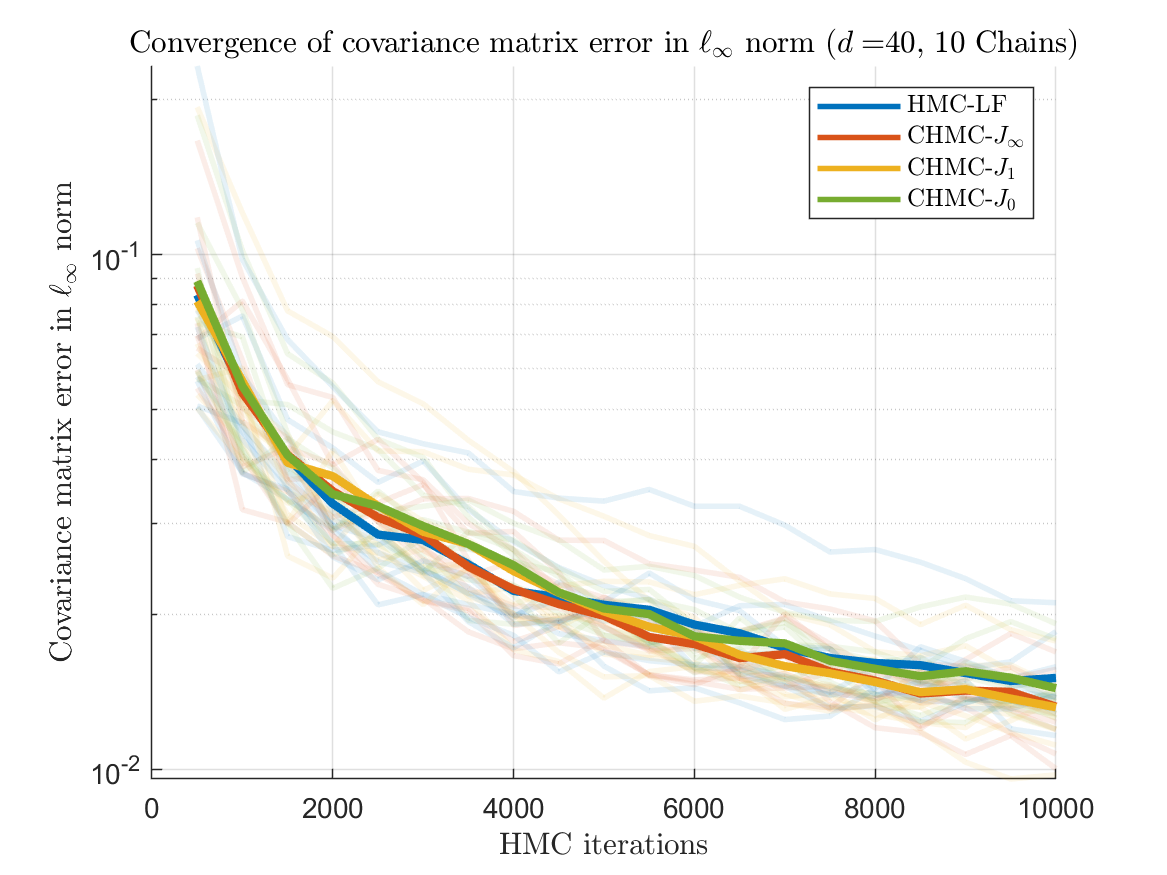
(a) $d=40$

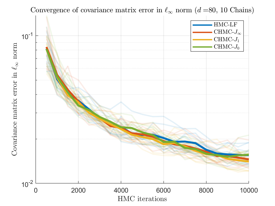
(b) $d=80$

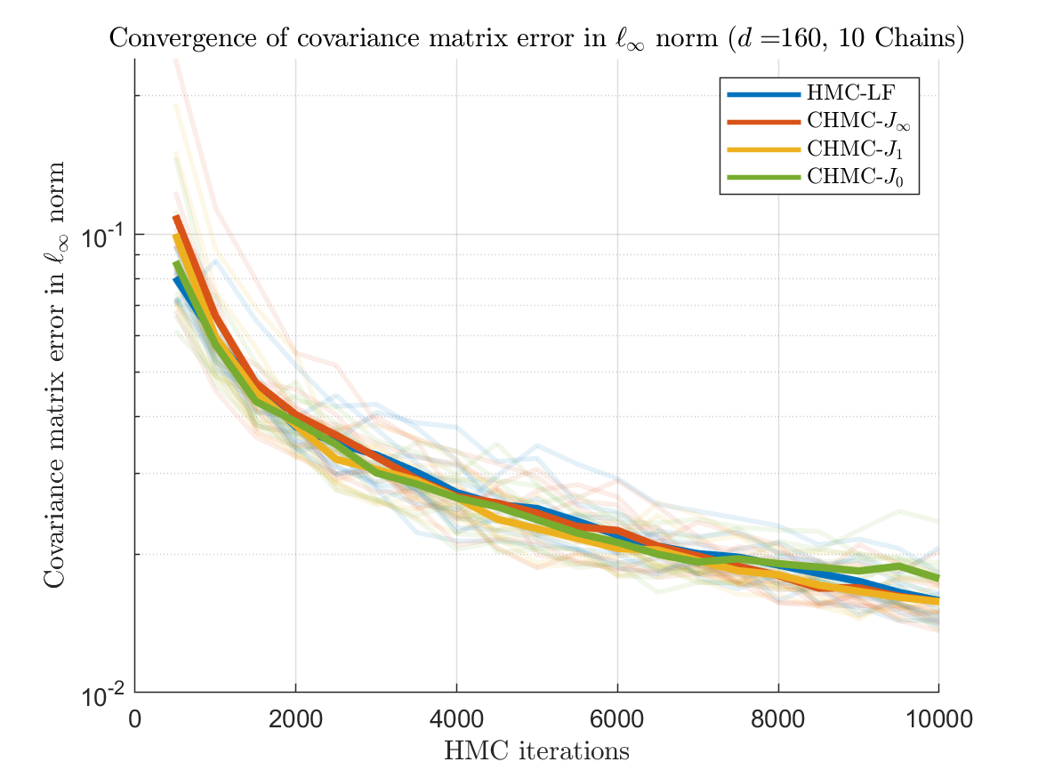
(c) $d=160$

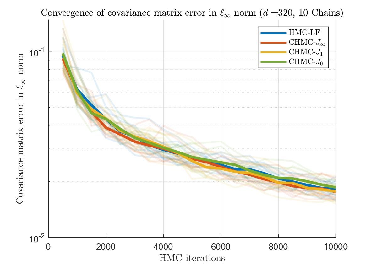
(d) $d=320$

Figure 1: Convergence in covariance matrix in logarithm scale is shown for the Generalized Gaussian distribution for $d=40,80,160$ and $320$ using HMC-Leapfrog, CHMC-$J_{0}$, CHMC-$J_{1}$ and CHMC-$J_{\infty}$. Each plot shows 10 chains and their corresponding average values, which are highlighted as solid lines for each method.

In Fig. 1, we see plots showing convergence of the sample covariance for HMC-Leapfrog and CHMC using $J_{0},J_{1}$ and $J_{\infty}$. A total of 10 chains was computed, with their corresponding averages shown as solid lines in each plot. The main takeaway from these results is that there is little to no difference between any of these methods in the convergence rate or asymptotic value after 10000 iterations.

	$d$	HMC-LF	CHMC-$J_{0}$	CHMC-$J_{1}$	CHMC-$J_{\infty}$
Mean Accept. Prob.	40	97.72	100.00	98.80	98.87
	80	96.80	100.00	98.34	98.48
	160	95.60	100.00	97.56	97.83
	320	94.184	100.00	96.425	96.92
Mean Energy Error	40	$4.82\times{10}^{-2}$	$4.62\times{10}^{-9}$	$4.57\times{10}^{-9}$	$4.58\times{10}^{-9}$
	80	$6.84\times{10}^{-2}$	$4.63\times{10}^{-9}$	$4.57\times{10}^{-9}$	$4.57\times{10}^{-9}$
	160	$9.839\times{10}^{-2}$	$3.86\times{10}^{-7}$	$3.86\times{10}^{-7}$	$3.86\times{10}^{-7}$
	320	$1.37\times{10}^{-1}$	$4.59\times{10}^{-9}$	$4.42\times{10}^{-9}$	$4.45\times{10}^{-9}$
Mean Force Eval.	40	2.000	7.124	7.121	7.121
	80	2.000	7.411	7.408	7.410
	160	2.000	7.678	7.676	7.675
	320	2.000	7.926	7.923	7.923
Running Time (s)	40	0.234	0.964	11.327	21.636
	80	0.288	1.157	38.252	80.882
	160	0.437	2.010	148.846	389.697
	320	0.583	2.902	471.230	1100.096

Table 2: Comparison of HMC-LF versus the three CHMC variants across various $d$ for mean acceptance probability, mean energy error, mean force evaluations and running time. The fixed point iteration of CHMC used an energy tolerance $\delta=1\times{10}^{-8}$ with a maximum of 10 fixed point iterations.

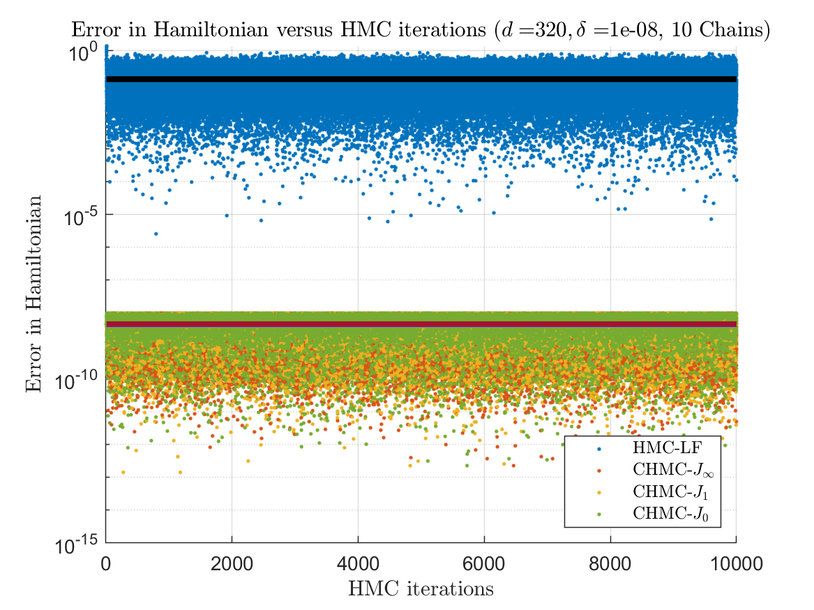
Figure 2: Error in the Hamiltonian associated with the Generalized Gaussian distribution across 10 chains in 320 dimensions during numerical integration using HMC-LF, CHMC-$J_{0}$, CHMC-$J_{1}$ and CHMC-$J_{\infty}$. The solid line indicates the average error across all chains.

Referencing Table 2 however, we begin to see significant differences in performance between the different CHMC methods. In particular we see significant increases in computation times for CHMC-$J_{1}$ and CHMC-$J_{\infty}$ and a slight reduction in acceptance rates as dimension increases. In contrast, the Gradient-free CHMC, denoted as CHMC-$J_{0}$, has comparable computation time to HMC-LF and maintains essentially a $100\%$ acceptance rate for all values of the dimension $d$.

Plots illustrating the error in the Hamiltonian and acceptance probabilities during numerical integration are illustrated in Fig. 2 and Fig. 3 respectively. The results presented thus far indicate that CHMC-$J_{0}$ is significantly more effective than our other proposed CHMC variants. Therefore for further results, we compare HMC-LF only with CHMC-$J_{0}$.

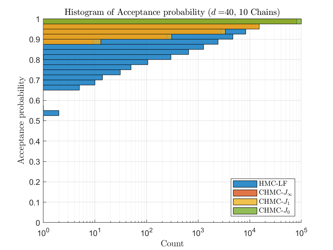
(a) $d=40$

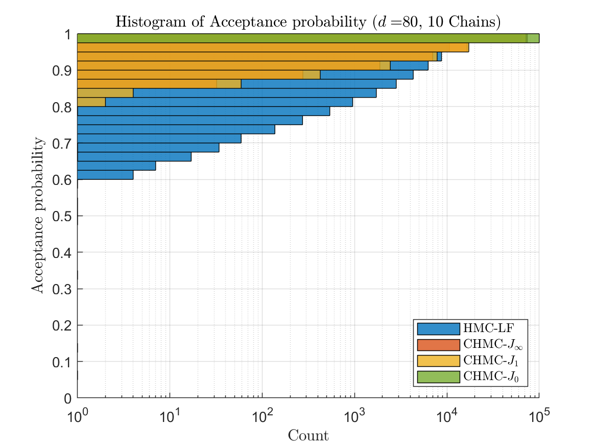
(b) $d=80$

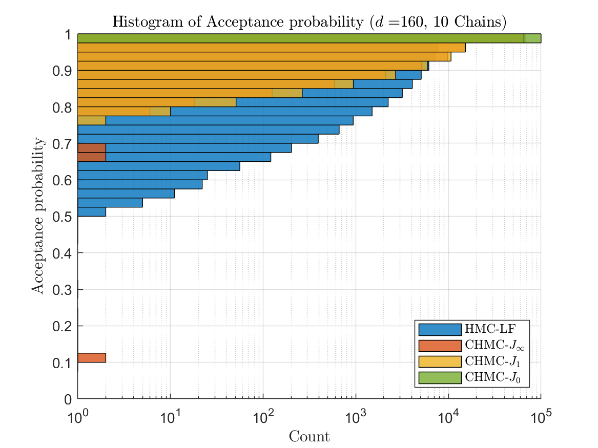
(c) $d=160$

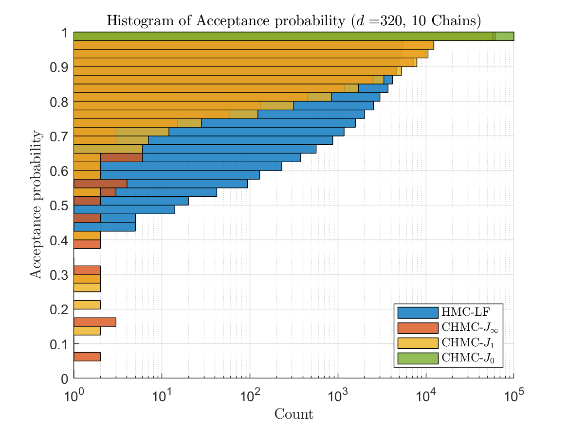
(d) $d=320$

Figure 3: Acceptance rate histograms for the Generalized Gaussian distribution across 10 chains for $d=40,80,160$ and $320$ using HMC-LF, CHMC-$J_{0}$, CHMC-$J_{1}$ and CHMC-$J_{\infty}$.

In the next set of results, we compare the sampling efficacy of CHMC-$J_{0}$ and HMC-LF using the same Generalized Gaussian distribution as above, for $d$ between 640 and 40960. To keep the computation times relatively close, we solve (25) using a maximum of 5 fixed point iterations instead of allowing iterations to continue until the tolerance $\delta$ is reached. Convergence of the error in the covariance matrix for $d=640,2560,$ $10240$ and $40960$ across 10 chains is shown in Fig. 4.

The results in Fig. 4 indicate that, for a fixed time step $\tau=0.1$, CHMC-$J_{0}$ achieves a significantly improved rate of convergence towards the stationary distribution over HMC-LF in high dimensional problems. One explanation for the distinct separation between the two methods is the dramatic decline in acceptance rate of the HMC-Leapfrog method.

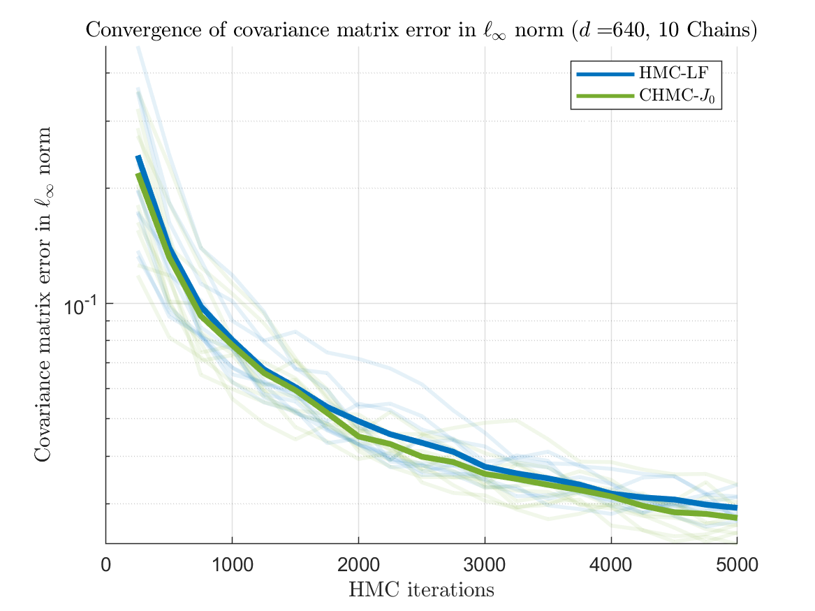
(a) $d=640$

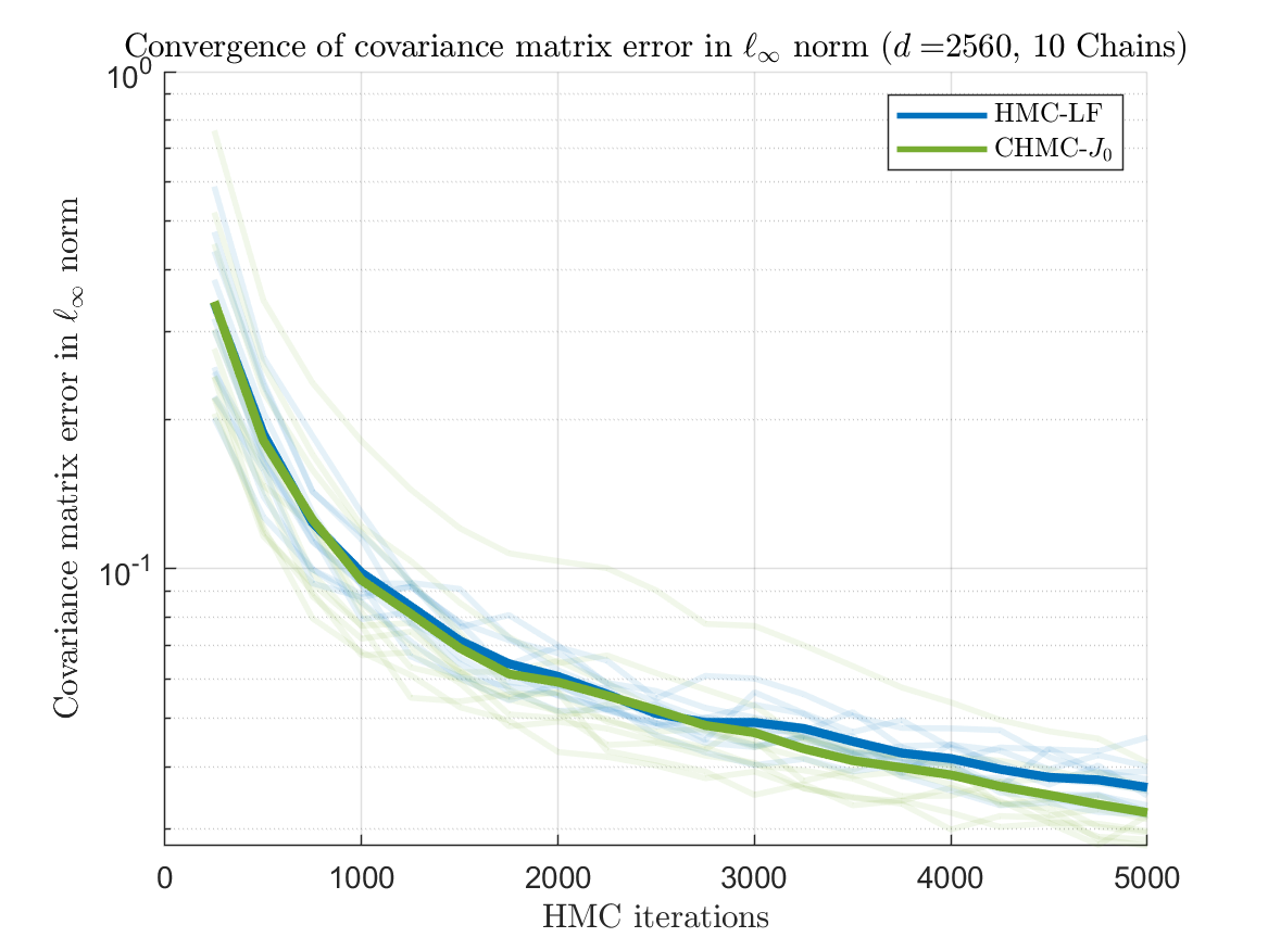
(b) $d=2560$

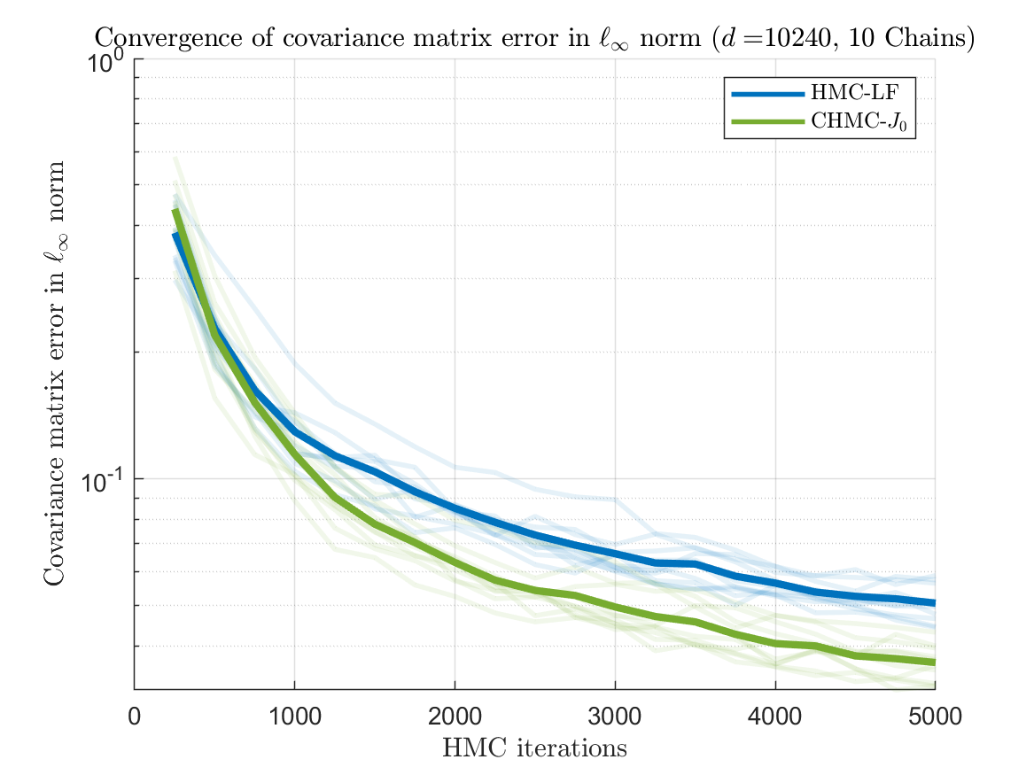
(c) $d=10240$

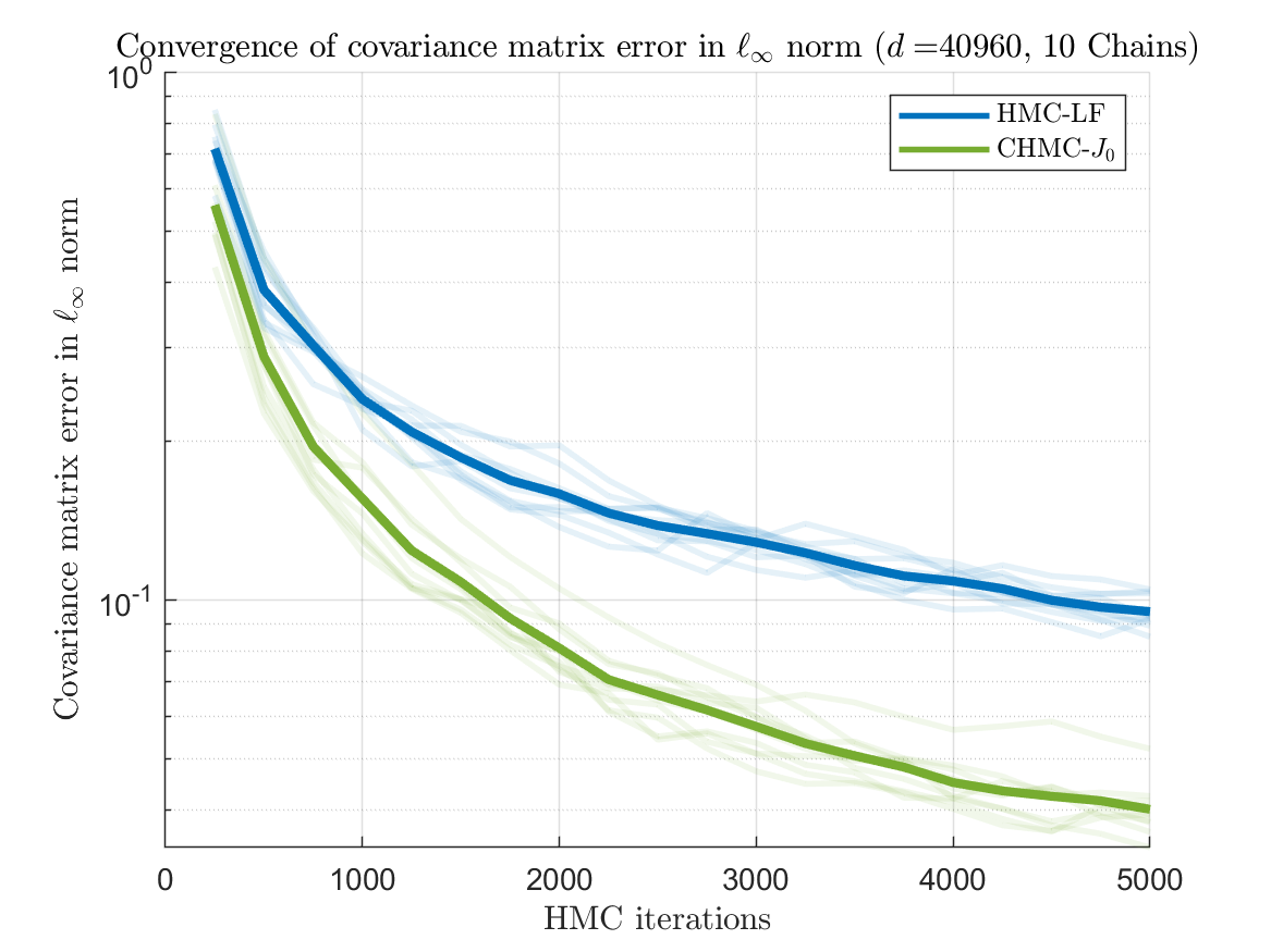
(d) $d=40960$

Figure 4: Convergence of covariance matrix in $\ell_{\infty}$ norm is shown on logarithmic scale for the Generalized Gaussian distribution for $d=640,2560,10240$ and $40960$. Plots of the corresponding average error over 10 chains are shown in solid.

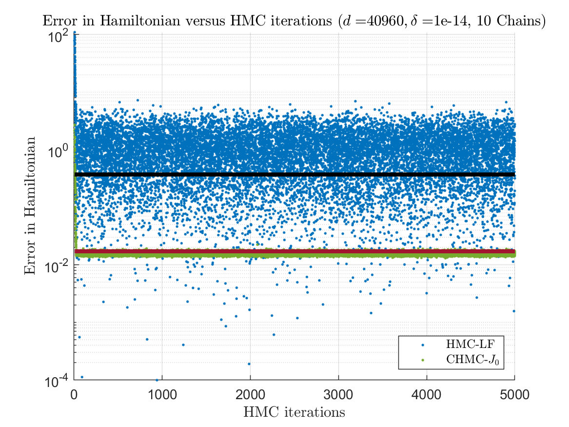
Figure 5: Error in the Hamiltonian associated with the Generalized Gaussian distribution across 10 chains in 40960 dimensions during numerical integration using HMC-LF and CHMC-$J_{0}$. The solid line indicates the average error across all chains.

Figure 5 shows the error in the Hamiltonian and Fig. 6 illustrates the decline of the acceptance probability as a set of histograms, highlighting the difference in the two methods as dimension increases.

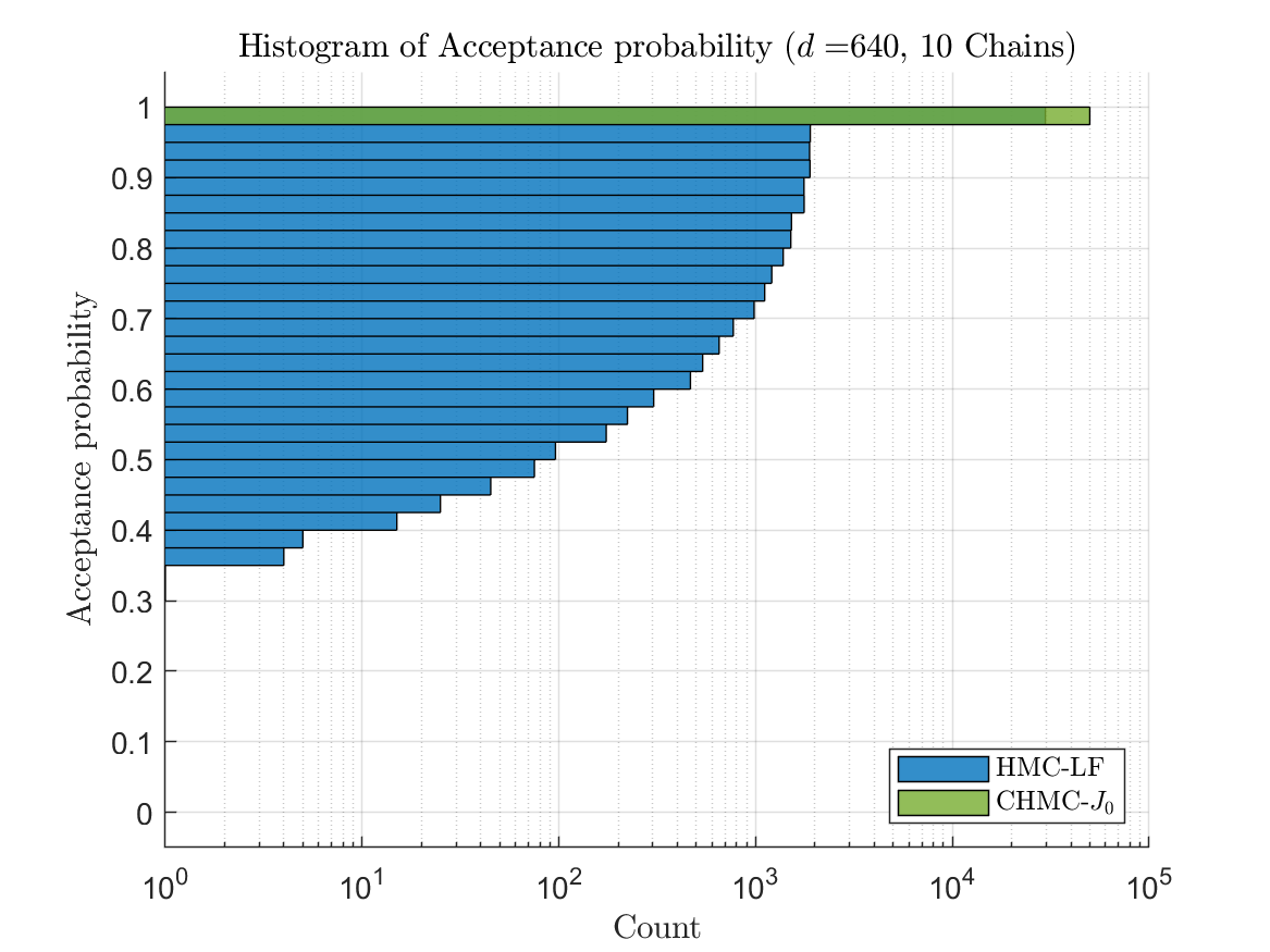
(a) $d=640$

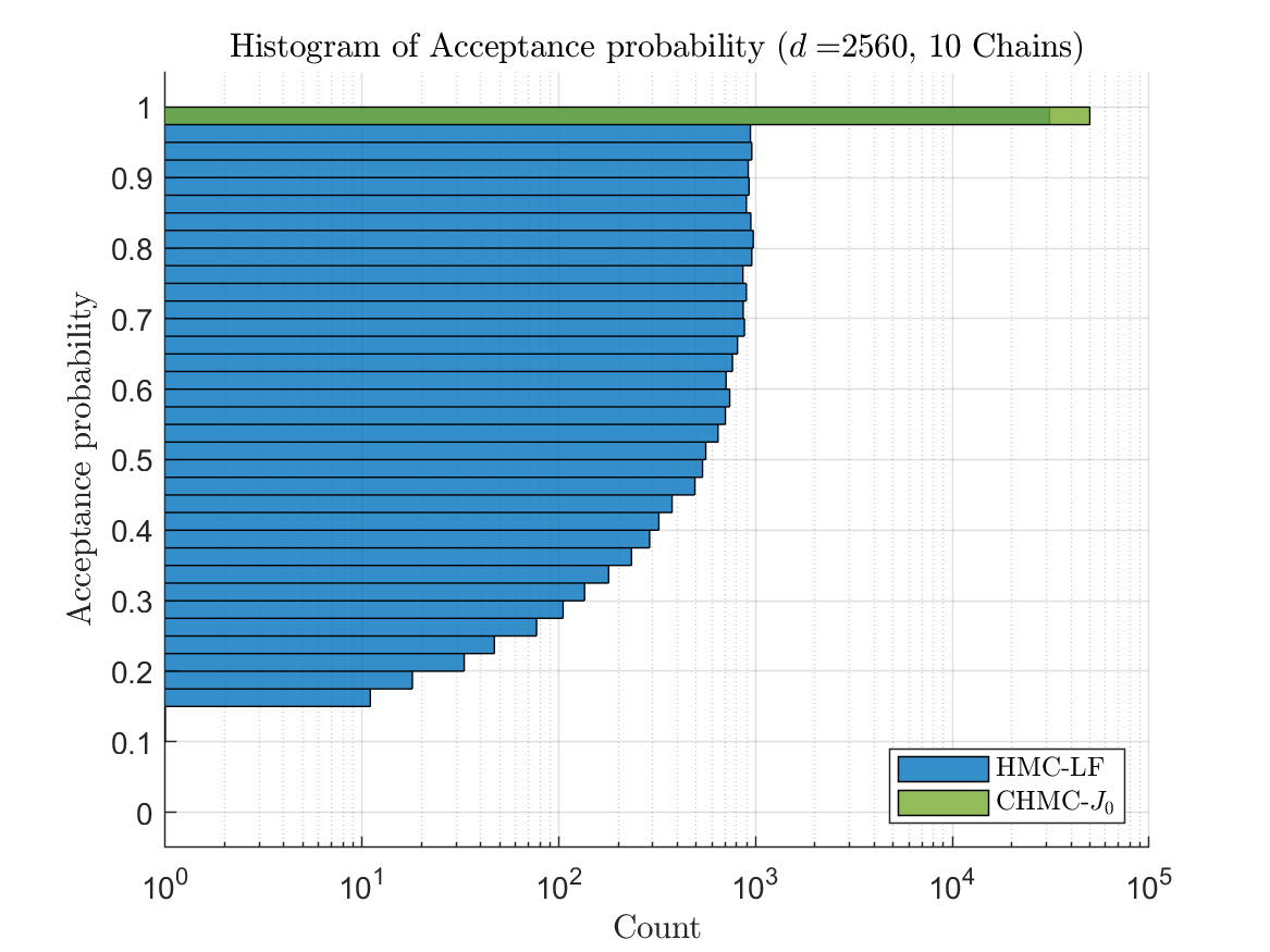
(b) $d=2560$

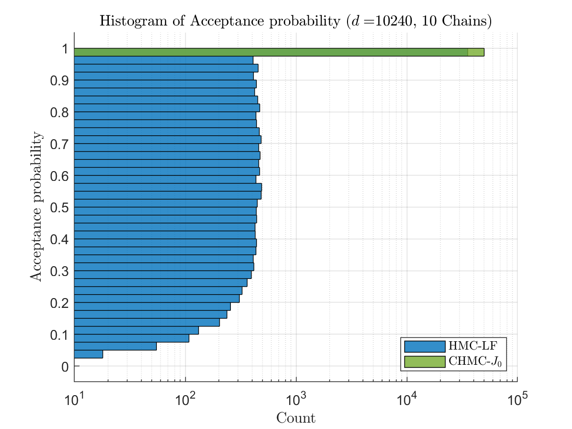
(c) $d=10240$

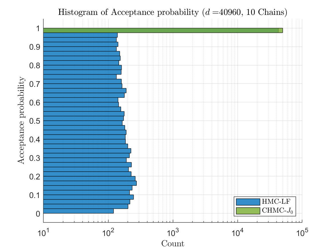
(d) $d=40960$

Figure 6: Acceptance rate histograms for the Generalized Gaussian distribution across 10 chains for $d=640,2560,10240$ and $40960$ using HMC-LF and CHMC-$J_{0}$.

4.2 Discussion of numerical results

In Section 4.1 we presented a detailed comparison of CHMC methods and HMC with Leapfrog. Taking the target distribution to be the generalized Gaussian distribution, we presented results showcasing the efficacy of the Gradient-free CHMC method with dramatic improvements in acceptance probability and convergence for high-dimensional problems. We note that while Leapfrog continues to be computationally more efficient, the higher rate of rejection allows the more expensive CHMC-$J_{0}$ to make up for its additional computational cost as the dimension increases. Furthermore, we have not incorporated the potential cost of computing the gradients required to employ Leapfrog to begin with. In practice, derivatives of $U$ can be expensive to compute in high dimensional problems, which may give the Gradient-free CHMC method a significant advantage over HMC with leapfrog in those cases.

5 Conclusion

In this paper, we have extended HMC to include the usage of energy-preserving schemes, leading to the introduction of the CHMC method. In doing so, an additional term involving the Jacobian matrix of the DMM scheme was needed in the acceptance probability of HMC to establish stationarity. However, through practical concerns and numerical experimentation, we observed that the Gradient-free CHMC yielded better acceptance probability and convergence properties than HMC with Leapfrog in high dimensional problems. Additionally, the gradient-free property of the Gradient-free CHMC method extends the applicability of HMC to a larger class of problems where gradient computation may be expensive or inaccessible in practice.

With the CHMC method established, we look forward to exploring future work on CHMC. An open problem we wish to understand is why the numerical results of the Gradient-free CHMC method does not appear to be impacted by its error in stationarity in practice. In a similar manner as tuning parameters of HMC, we wish to study and optimize the role of tuning the energy error tolerance $\delta$, step size $\tau$, and integration time $T$, in a similar manner as how $\tau\propto\mathcal{O}(d^{-\frac{1}{4}})$ in HMC and No-U-Turn sampling of HMC. Futhermore, another open problem is to incorporate a ${\boldsymbol{q}}$ dependant mass matrix $M({\boldsymbol{q}})$ for CHMC, leading to the possibility of Riemannian CHMC in a similar manner to Riemannian HMC. Moreover, we wish to test the efficacy of the Gradient-free CHMC method in practice, specifically for high dimensional applications in parameter estimation and machine learning, such as Bayesian statistics and Bayesian neural networks. Moreover, to facilitate the use of CHMC for a wide range of problems, it would be advantageous to implement CHMC in established statistics packages, such as Stan [9].

Appendix A Appendix

A.1 Calculation of the symmetrized DMM Scheme

Proof A.1.

For a separable Hamiltonian of the form $H({\boldsymbol{q}},{\boldsymbol{p}})=K({\boldsymbol{p}})+U({\boldsymbol{q}})$, a symmetric DMM scheme [39] using divided differences is

$$Q_{i} =q_{i}+\frac{\tau}{2}\left(\frac{K(\hat{{\boldsymbol{P}}}^{i})-K(\hat{{\boldsymbol{P}}}^{i-1})}{P_{i}-p_{i}}+\frac{K(\hat{{\boldsymbol{p}}}^{i-1})-K(\hat{{\boldsymbol{p}}}^{i})}{P_{i}-p_{i}}\right),$$

$$P_{i} =p_{i}-\frac{\tau}{2}\left(\frac{U(\hat{{\boldsymbol{Q}}}^{i})-U(\hat{{\boldsymbol{Q}}}^{i-1})}{Q_{i}-q_{i}}+\frac{U(\hat{{\boldsymbol{q}}}^{i-1})-U(\hat{{\boldsymbol{q}}}^{i})}{Q_{i}-q_{i}}\right).$$

Therefore, taking $K({\boldsymbol{p}})=\frac{1}{2}{\boldsymbol{p}}^{T}M^{-1}{\boldsymbol{p}}$ we obtain

(26)

To simplify the $Q_{i}$ equations, we use the identity ${\boldsymbol{x}}^{T}A{\boldsymbol{x}}-{\boldsymbol{y}}^{T}A{\boldsymbol{y}}=({\boldsymbol{x}}+{\boldsymbol{y}})^{T}A({\boldsymbol{x}}-{\boldsymbol{y}})$ for any ${\boldsymbol{x}},{\boldsymbol{y}}\in\mathbb{R}^{d}$ and real symmetric matrix $A$. Then, using $\hat{{\boldsymbol{P}}}^{i}-\hat{{\boldsymbol{P}}}^{i-1}=(P_{i}-p_{i}){\boldsymbol{e}}_{i}$, and similarly $\hat{{\boldsymbol{p}}}^{i-1}-\hat{{\boldsymbol{p}}}^{i}=(P_{i}-p_{i}){\boldsymbol{e}}_{i}$, where ${\boldsymbol{e}}_{i}$ denotes the $i$-th standard basis vector, the $Q_{i}$ equations become

$$\begin{split}Q_{i}&=q_{i}+\frac{\tau}{4}\left(\left(\hat{{\boldsymbol{P}}}^{i}+\hat{{\boldsymbol{P}}}^{i-1}\right)^{T}M^{-1}{\boldsymbol{e}}_{i}+\left(\hat{{\boldsymbol{p}}}^{i-1}+\hat{{\boldsymbol{p}}}^{i}\right)^{T}M^{-1}{\boldsymbol{e}}_{i}\right)\\ &=q_{i}+\frac{\tau}{4}\left(\left(\hat{{\boldsymbol{P}}}^{i}+\hat{{\boldsymbol{P}}}^{i-1}+\hat{{\boldsymbol{p}}}^{i-1}+\hat{{\boldsymbol{p}}}^{i}\right)^{T}M^{-1}{\boldsymbol{e}}_{i}\right).\end{split}$$

Finally, using that $\hat{{\boldsymbol{P}}}^{i}+\hat{{\boldsymbol{P}}}^{i-1}+\hat{{\boldsymbol{P}}}^{i-1}+\hat{{\boldsymbol{P}}}^{i}=2\left({\boldsymbol{P}}+{\boldsymbol{p}}\right)$, the DMM scheme (26) for the Hamiltonian system (4) can be simplified to (8).

A.2 Proof of Lemma 2.1

Proof A.2.

Rewriting the $P_{i}$ equation from (8), we obtain

$$2\frac{(Q_{i}-q_{i})(P_{i}-p_{i})}{\tau}=-U(\hat{{\boldsymbol{Q}}}^{i})+U(\hat{{\boldsymbol{Q}}}^{i-1})-U(\hat{{\boldsymbol{q}}}^{i-1})+U(\hat{{\boldsymbol{q}}}^{i}).$$

Substituting $Q_{i}-q_{i}$ using equation (26), and denoting $K({\boldsymbol{p}})=\frac{1}{2}{{\boldsymbol{p}}}^{T}M^{-1}{\boldsymbol{p}}$ as the kinetic energy, we obtain

$$K(\hat{{\boldsymbol{P}}}^{i})-K(\hat{{\boldsymbol{P}}}^{i-1})+K(\hat{{\boldsymbol{p}}}^{i-1})-K(\hat{{\boldsymbol{p}}}^{i})=U(\hat{{\boldsymbol{Q}}}^{i-1})-U(\hat{{\boldsymbol{Q}}}^{i})+U(\hat{{\boldsymbol{q}}}^{i})-U(\hat{{\boldsymbol{q}}}^{i-1}).$$

Summing this equation from $i=1$ to $i=d$, and noting the telescoping sum on both sides of the equation yields

$$K(\hat{{\boldsymbol{P}}}^{d})-K(\hat{{\boldsymbol{P}}}^{0})+K(\hat{{\boldsymbol{p}}}^{0})-K(\hat{{\boldsymbol{p}}}^{d})=U(\hat{{\boldsymbol{Q}}}^{0})-U(\hat{{\boldsymbol{Q}}}^{d})+U(\hat{{\boldsymbol{q}}}^{d})-U(\hat{{\boldsymbol{q}}}^{0}).$$

Finally, recalling that $\hat{{\boldsymbol{P}}}^{d}={\boldsymbol{P}},\hat{{\boldsymbol{P}}}^{0}={\boldsymbol{p}},\hat{{\boldsymbol{p}}}^{d}={\boldsymbol{p}},\hat{{\boldsymbol{p}}}^{0}={\boldsymbol{P}}$, the corresponding identities for $\hat{{\boldsymbol{Q}}}^{i}$, and that $H({\boldsymbol{q}},{\boldsymbol{p}})=U({\boldsymbol{q}})+K({\boldsymbol{p}})$ we obtain the desired result that $H({\boldsymbol{Q}},{\boldsymbol{P}})-H({\boldsymbol{q}},{\boldsymbol{p}})=0$.

A.3 Proof of Lemma 2.2

Proof A.3.

We begin by computing $\Psi_{D}^{-1}$, which exists by the implicit function theorem. Referring to the formulas (7) and the DMM scheme (8), we obtain

$$\Psi_{D}^{-1}({\boldsymbol{q}},{\boldsymbol{p}}):\quad\left\{\!\begin{aligned} q_{i}&=Q_{i}+\frac{\tau}{2}\left({\boldsymbol{p}}+{\boldsymbol{P}}\right)^{T}M^{-1}{\boldsymbol{e}}_{i}\\ p_{i}&=P_{i}-\frac{\tau}{2}\left(\frac{U(\hat{{\boldsymbol{q}}}^{i})-U(\hat{{\boldsymbol{q}}}^{i-1})}{q_{i}-Q_{i}}+\frac{U(\hat{{\boldsymbol{Q}}}^{i-1})-U(\hat{{\boldsymbol{Q}}}^{i})}{q_{i}-Q_{i}}\right).\end{aligned}\right.$$

Rearranging the equations, we obtain

(27) $$\Psi_{D}^{-1}({\boldsymbol{q}},{\boldsymbol{p}}):\quad\left\{\!\begin{aligned} Q_{i}&=q_{i}-\frac{\tau}{2}\left({\boldsymbol{P}}+{\boldsymbol{p}}\right)^{T}M^{-1}{\boldsymbol{e}}_{i}\\ P_{i}&=p_{i}+\frac{\tau}{2}\left(\frac{U(\hat{{\boldsymbol{Q}}}^{i})-U(\hat{{\boldsymbol{Q}}}^{i-1})}{Q_{i}-q_{i}}+\frac{U(\hat{{\boldsymbol{q}}}^{i-1})-U(\hat{{\boldsymbol{q}}}^{i})}{Q_{i}-q_{i}}\right).\end{aligned}\right.$$

Next we show that $R\circ\Psi_{D}\circ R=\Psi_{D}^{-1}$. Computing $R\circ\Psi_{D}\circ R$, we obtain

(28) $$R\circ\Psi_{D}\circ R({\boldsymbol{q}},{\boldsymbol{p}}):\quad\left\{\!\begin{aligned} Q_{i}&=q_{i}+\frac{\tau}{2}\left(-{\boldsymbol{P}}-{\boldsymbol{p}}\right)^{T}M^{-1}{\boldsymbol{e}}_{i}\\ -P_{i}&=-p_{i}-\frac{\tau}{2}\left(\frac{U(\hat{{\boldsymbol{Q}}}^{i})-U(\hat{{\boldsymbol{Q}}}^{i-1})}{Q_{i}-q_{i}}+\frac{U(\hat{{\boldsymbol{q}}}^{i-1})-U(\hat{{\boldsymbol{q}}}^{i})}{Q_{i}-q_{i}}\right).\end{aligned}\right.$$

Multiplying the $P_{i}$ equations by $-1$, we obtain the same mapping as $\Psi_{D}^{-1}({\boldsymbol{q}},{\boldsymbol{p}})$. Thus, we have shown $R\circ\Psi_{D}\circ R\circ\Psi_{D}=I$ as desired.

A.4 Proof of Corollary 2.3

Proof A.4.

Since $R\circ R=I$ and $R\circ\Psi\circ R=\Psi^{-1}$,

$$R\circ\Psi^{k}\circ R=R\circ(\Psi\circ R\circ R)^{k}\circ R=R\circ\overbrace{(\Psi\circ R\circ R)\circ\cdots\circ(\Psi\circ R\circ R)}^{k~{}\text{times}}\circ R$$

$$=\underbrace{(R\circ\Psi\circ R)\circ\cdots\circ(R\circ\Psi\circ R)}_{k~{}\text{times}}\circ R\circ R=(R\circ\Psi\circ R)^{k}\circ I=(\Psi^{-1})^{k}=(\Psi^{k})^{-1}$$

A.5 Proof of Lemma 2.4

Proof A.5.

We first prove (10). In vector form, the map $\Psi_{D}$ can be written as

(29) $$\begin{split}{\boldsymbol{Q}}&={\boldsymbol{q}}+\frac{\tau}{2}M^{-1}({\boldsymbol{P}}+{\boldsymbol{p}})\\ {\boldsymbol{P}}&={\boldsymbol{p}}-\frac{\tau}{2}{\boldsymbol{F}}({\boldsymbol{Q}},{\boldsymbol{q}}),\end{split}$$

where the components of ${\boldsymbol{F}}$ are given by (9).

Plugging the equation for ${\boldsymbol{P}}$ into ${\boldsymbol{Q}}$ of (29), we obtain the system

$$\begin{split}{\boldsymbol{Q}}&={\boldsymbol{q}}+\frac{\tau}{2}(2{\boldsymbol{p}}-\frac{\tau}{2}M^{-1}{\boldsymbol{F}}({\boldsymbol{Q}},{\boldsymbol{q}})),\\ {\boldsymbol{P}}&={\boldsymbol{p}}-\frac{\tau}{2}{\boldsymbol{F}}({\boldsymbol{Q}},{\boldsymbol{q}}),\end{split}$$

which allows straight-forward computations of the partial derivatives $\dfrac{\partial{\boldsymbol{Q}}}{\partial{\boldsymbol{q}}}$ and $\dfrac{\partial{\boldsymbol{Q}}}{\partial{\boldsymbol{p}}}$, given by

(30) $$\begin{split}\left(I+\frac{\tau^{2}}{4}M^{-1}D_{{\boldsymbol{Q}}}{\boldsymbol{F}}\right)\frac{\partial{\boldsymbol{Q}}}{\partial{\boldsymbol{q}}}&=I-\frac{\tau^{2}}{4}M^{-1}D_{{\boldsymbol{q}}}{\boldsymbol{F}},\\ \left(I+\frac{\tau^{2}}{4}M^{-1}D_{{\boldsymbol{Q}}}{\boldsymbol{F}}\right)\frac{\partial{\boldsymbol{Q}}}{\partial{\boldsymbol{p}}}&=\tau M^{-1}.\end{split}$$

Computing $\dfrac{\partial{\boldsymbol{P}}}{\partial{\boldsymbol{q}}}$ and $\dfrac{\partial{\boldsymbol{P}}}{\partial{\boldsymbol{p}}}$ using equation (29), and plugging in $\dfrac{\partial{\boldsymbol{Q}}}{\partial{\boldsymbol{q}}}$ and $\dfrac{\partial{\boldsymbol{Q}}}{\partial{\boldsymbol{p}}}$ obtained from differentiating the ${\boldsymbol{Q}}$ equation from (29) directly, we obtain

(31) $$\begin{split}\left(I+\frac{\tau^{2}}{4}M^{-1}D_{{\boldsymbol{Q}}}{\boldsymbol{F}}\right)\frac{\partial{\boldsymbol{P}}}{\partial{\boldsymbol{q}}}&=-\frac{\tau}{2}(D_{{\boldsymbol{Q}}}{\boldsymbol{F}}+D_{{\boldsymbol{q}}}{\boldsymbol{F}}),\\ \left(I+\frac{\tau^{2}}{4}M^{-1}D_{{\boldsymbol{Q}}}{\boldsymbol{F}}\right)\frac{\partial{\boldsymbol{P}}}{\partial{\boldsymbol{p}}}&=I-\frac{\tau^{2}}{4}M^{-1}D_{{\boldsymbol{Q}}}{\boldsymbol{F}}.\end{split}$$

Using (30) and (31), we obtain an expression for $J=\begin{pmatrix}\frac{\partial{\boldsymbol{Q}}}{\partial{\boldsymbol{q}}}&\frac{\partial{\boldsymbol{Q}}}{\partial{\boldsymbol{p}}}\\ \frac{\partial{\boldsymbol{P}}}{\partial{\boldsymbol{q}}}&\frac{\partial{\boldsymbol{P}}}{\partial{\boldsymbol{p}}}\end{pmatrix}$, given by $\begin{pmatrix}I+\frac{\tau^{2}}{4}M^{-1}D_{{\boldsymbol{Q}}}{\boldsymbol{F}}&{\boldsymbol{0}}\\ {\boldsymbol{0}}&I+\frac{\tau^{2}}{4}M^{-1}D_{{\boldsymbol{Q}}}{\boldsymbol{F}}\end{pmatrix}^{-1}\begin{pmatrix}I-\frac{\tau^{2}}{4}M^{-1}D_{{\boldsymbol{q}}}{\boldsymbol{F}}&\tau M^{-1}\\ -\frac{\tau}{2}\left(D_{{\boldsymbol{Q}}}{\boldsymbol{F}}+D_{{\boldsymbol{q}}}{\boldsymbol{F}}\right)&I-\frac{\tau^{2}}{4}M^{-1}D_{{\boldsymbol{Q}}}{\boldsymbol{F}}\end{pmatrix}.$
Therefore, we obtain the equation for the determinant of $J$ given by

(32) $$\det J=\frac{\det\begin{pmatrix}I-\frac{\tau^{2}}{4}M^{-1}D_{{\boldsymbol{q}}}{\boldsymbol{F}}&\tau M^{-1}\\ -\frac{\tau}{2}\left(D_{{\boldsymbol{Q}}}{\boldsymbol{F}}+D_{{\boldsymbol{q}}}{\boldsymbol{F}}\right)&I-\frac{\tau^{2}}{4}M^{-1}D_{{\boldsymbol{Q}}}{\boldsymbol{F}}\end{pmatrix}}{\det\left(I+\frac{\tau^{2}}{4}M^{-1}D_{{\boldsymbol{Q}}}{\boldsymbol{F}}\right)^{2}}.$$

To compute the determinant of the numerator, we rewrite the matrix as the product

(33) $$\begin{pmatrix}M^{-1}&0\\ 0&I\end{pmatrix}.\begin{pmatrix}M-\frac{\tau^{2}}{4}D_{{\boldsymbol{q}}}{\boldsymbol{F}}&\tau I\\ -\frac{\tau}{2}\left(D_{{\boldsymbol{Q}}}{\boldsymbol{F}}+D_{{\boldsymbol{q}}}{\boldsymbol{F}}\right)&I-\frac{\tau^{2}}{4}M^{-1}D_{{\boldsymbol{Q}}}{\boldsymbol{F}}\end{pmatrix}$$

Recalling a well-known result for block matrices, $\det\begin{pmatrix}A&B\\ C&D\end{pmatrix}=\det(AD-BC)$ provided $BC=CB$, we observe that $\tau I$ commutes with $-\frac{\tau}{2}\left(D_{{\boldsymbol{Q}}}{\boldsymbol{F}}+D_{{\boldsymbol{q}}}{\boldsymbol{F}}\right)$, and thus

(34) $$\det\begin{pmatrix}M-\frac{\tau^{2}}{4}D_{{\boldsymbol{q}}}{\boldsymbol{F}}&\tau I\\ -\frac{\tau}{2}\left(D_{{\boldsymbol{Q}}}{\boldsymbol{F}}+D_{{\boldsymbol{q}}}{\boldsymbol{F}}\right)&I-\frac{\tau^{2}}{4}M^{-1}D_{{\boldsymbol{Q}}}{\boldsymbol{F}}\end{pmatrix}$$

$$=\det\left(\left(M-\frac{\tau^{2}}{4}D_{{\boldsymbol{q}}}{\boldsymbol{F}}\right)\left(I-\frac{\tau^{2}}{4}M^{-1}D_{{\boldsymbol{Q}}}{\boldsymbol{F}}\right)+\frac{\tau^{2}}{2}\left(D_{{\boldsymbol{Q}}}{\boldsymbol{F}}+D_{{\boldsymbol{q}}}{\boldsymbol{F}}\right)\right)$$

$$=\det\left(M\left(I+\frac{\tau^{2}}{4}M^{-1}D_{{\boldsymbol{q}}}{\boldsymbol{F}}\right)\left(I+\frac{\tau^{2}}{4}M^{-1}D_{{\boldsymbol{Q}}}{\boldsymbol{F}}\right)\right).$$

Combining (32), (33) and (34) gives the desired first result of this Lemma,

$$\det J =\frac{\det\left(I+\frac{\tau^{2}}{4}M^{-1}D_{{\boldsymbol{q}}}{\boldsymbol{F}}\right)\left(I+\frac{\tau^{2}}{4}M^{-1}D_{{\boldsymbol{Q}}}{\boldsymbol{F}}\right)}{\det\left(I+\frac{\tau^{2}}{4}M^{-1}D_{{\boldsymbol{Q}}}{\boldsymbol{F}}\right)^{2}}=\frac{\det\left(1+\frac{\tau^{2}}{4}M^{-1}D_{{\boldsymbol{q}}}{\boldsymbol{F}}\right)}{\det\left(1+\frac{\tau^{2}}{4}M^{-1}D_{{\boldsymbol{Q}}}{\boldsymbol{F}}\right)}.$$

Next, we prove the expansion of the above determinant given by (11). Using well-known Newton’s identities, we have for $s\in\mathbb{R}$ and any $d\times d$ matrices $A,B$,

$$\det(I+sA)=I+sTr(A)+\frac{s^{2}}{2}\left(Tr(A)^{2}-Tr(A^{2})\right)+O(s^{3}),$$

which yields for (10) upon division by analytic functions and simplifications,

$$\frac{\det(I+sA)}{\det(I+sB)}= 1+s(Tr(A)-Tr(B))+\frac{s^{2}}{2}\left((Tr(A)^{2}-Tr(B)^{2})+Tr(B^{2}-A^{2})\right)$$

$$\hskip 5.69054pt-s^{2}\left(Tr(B)(Tr(A)-Tr(B))\right)+O(s^{3})$$

$$= 1+sTr(A-B)+\frac{s^{2}}{2}\left((Tr(B-A))^{2}+Tr(B^{2}-A^{2})\right)+O(s^{3}).$$

Applying this to (10) with $s=\frac{1}{4}\tau^{2},A=M^{-1}D_{{\boldsymbol{q}}}{\boldsymbol{F}}$ and $B=M^{-1}D_{{\boldsymbol{Q}}}{\boldsymbol{F}}$ yields

$$\det J=1 +\frac{\tau^{2}}{4}Tr\left(M^{-1}(D_{{\boldsymbol{q}}}{\boldsymbol{F}}-D_{{\boldsymbol{Q}}}{\boldsymbol{F}})\right)+\frac{\tau^{4}}{32}\left(Tr\left(M^{-1}(D_{{\boldsymbol{Q}}}{\boldsymbol{F}}-D_{{\boldsymbol{q}}}{\boldsymbol{F}})\right)\right)^{2}$$

$$+\frac{\tau^{4}}{32}\left(Tr((M^{-1}D_{{\boldsymbol{q}}}{\boldsymbol{F}})^{2}-(M^{-1}D_{{\boldsymbol{Q}}}{\boldsymbol{F}})^{2})\right)+O(\tau^{6}).$$

References

• [1] C. Andrieu, N. de Freitas, A. Doucet, and M. I. Jordan, An Introduction to MCMC for Machine Learning, Machine Learning, 50 (2003), pp. 5–43.
• [2] C. Andrieu and G. O. Roberts, The pseudo-marginal approach for efficient Monte Carlo computations, The Annals of Statistics, 37 (2009), pp. 697 – 725.
• [3] S. Banach, Sur les opérations dans les ensembles abstraits et leur application aux équations intégrales, Fund. math, 3 (1922), pp. 133–181.
• [4] A. Beskos, N. Pillai, G. Roberts, J.-M. Sanz-Serna, and A. Stuart, Optimal tuning of the hybrid Monte Carlo algorithm, Bernoulli, 19 (2013), pp. 1501–1534.
• [5] M. Betancourt, A conceptual introduction to Hamiltonian Monte Carlo, arXiv preprint arXiv:1701.02434, (2017).
• [6] S. Blanes, F. Casas, and J. M. Sanz-Serna, Numerical integrators for the Hybrid Monte Carlo method, SIAM Journal on Scientific Computing, 36 (2014), pp. A1556–A1580.
• [7] N. Bou-Rabee and J. M. Sanz-Serna, Geometric integrators and the Hamiltonian Monte Carlo method, Acta Numerica, 27 (2018), pp. 113–206.
• [8] S. P. Brooks and A. Gelman, General Methods for Monitoring Convergence of Iterative Simulations, Journal of Computational and Graphical Statistics, 7 (1998), pp. 434–455.
• [9] B. Carpenter, A. Gelman, M. D. Hoffman, D. Lee, B. Goodrich, M. Betancourt, M. Brubaker, J. Guo, P. Li, A. Riddell, et al., Stan: A probabilistic programming language, Journal of Statistical Software, 76 (2017).
• [10] C. K. Carter and R. Kohn, On Gibbs sampling for state space models, Biometrika, 81 (1994), pp. 541–553.
• [11] Celledoni, Elena, McLachlan, Robert I., McLaren, David I., Owren, Brynjulf, Reinout W. Quispel, G., and Wright, William M., Energy-preserving runge-kutta methods, ESAIM: M2AN, 43 (2009), pp. 645–649.
• [12] A. D. Cobb and B. Jalaian, Scaling Hamiltonian Monte Carlo Inference for Bayesian Neural Networks with Symmetric Splitting, arXiv preprint arXiv:2010.06772, (2020).
• [13] K.-D. Dang, M. Quiroz, R. Kohn, T. Minh-Ngoc, and M. Villani, Hamiltonian Monte Carlo with energy conserving subsampling, Journal of machine learning research, 20 (2019).
• [14] S. Duane, A. D. Kennedy, B. J. Pendleton, and D. Roweth, Hybrid Monte Carlo, Physics letters B, 195 (1987), pp. 216–222.
• [15] Y. Fang, J.-M. Sanz-Serna, and R. D. Skeel, Compressible Generalized Hybrid Monte Carlo, The Journal of chemical physics, 140 (2014), p. 174108.
• [16] A. E. Gelfand and A. F. M. Smith, Sampling-Based Approaches to Calculating Marginal Densities, Journal of the American Statistical Association, 85 (1990), pp. 398–409.
• [17] A. Gelman, J. B. Carlin, H. S. Stern, D. B. Rubin, D. Dunson, and A. Vehtari, Bayesian Data Analysis, Chapman and Hall/CRC, 3rd ed., 1995-2020.
• [18] E. I. George and R. E. McCulloch, Variable selection via Gibbs sampling, Journal of the American Statistical Association, 88 (1993), pp. 881–889.
• [19] M. Girolami and B. Calderhead, Riemann manifold Langevin and Hamiltonian Monte Carlo methods, Journal of the Royal Statistical Society: Series B (Statistical Methodology), 73 (2011), pp. 123–214.
• [20] C. Gormezano, J.-C. Nave, and A. T. S. Wan, Conservative Integrators for Vortex Blob Methods on the Plane, To appear in Journal of Computational Physics, arXiv preprint arXiv:2111.01233, (2021).
• [21] E. Hairer, C. Lubich, and G. Wanner, Geometric numerical integration: structure-preserving algorithms for ordinary differential equations, Springer, Berlin, 2006.
• [22] W. K. Hastings, Monte Carlo sampling methods using Markov chains and their applications, (1970).
• [23] A. Hirani, A. T. S. Wan, and W. Nikolas, Conservative Integrators for Piecewise Smooth Systems, arXiv preprint arXiv:2106.07484, (2021).
• [24] M. D. Hoffman, A. Gelman, et al., The No-U-Turn sampler: adaptively setting path lengths in Hamiltonian Monte Carlo., J. Mach. Learn. Res., 15 (2014), pp. 1593–1623.
• [25] T. Itoh and K. Abe, Hamiltonian-conserving discrete canonical equations based on variational difference quotients, Journal of Computational Physics, 76 (1988), pp. 85–102.
• [26] G. L. Jones, On the Markov chain central limit theorem, Probability Surveys, 1 (2004), pp. 299–320.
• [27] L. V. Jospin, W. L. Buntine, F. Boussaïd, H. Laga, and M. Bennamoun, Hands-on Bayesian Neural Networks - a Tutorial for Deep Learning Users, arXiv preprint arXiv:2007.06823, abs/ (2020).
• [28] F. Kang and S. Zai-jiu, Volume-preserving algorithms for source-free dynamical systems, Numerische Mathematik, 71 (1995), pp. 451–463.
• [29] P. Marjoram, J. Molitor, V. Plagnol, and S. Tavaré, Markov chain Monte Carlo without likelihoods, Proceedings of the National Academy of Sciences, 100 (2003), pp. 15324–15328.
• [30] R. I. McLachlan, G. R. W. Quispel, and N. Robidoux, Geometric integration using discrete gradients, Philosophical Transactions: Mathematical, Physical and Engineering Sciences, 357 (1999), pp. 1021–1045.
• [31] N. Metropolis, A. W. Rosenbluth, M. N. Rosenbluth, A. H. Teller, and E. Teller, Equation of state calculations by fast computing machines, The journal of chemical physics, 21 (1953), pp. 1087–1092.
• [32] R. M. Neal, An improved acceptance procedure for the hybrid Monte Carlo algorithm, Journal of Computational Physics, 111 (1994), pp. 194–203.
• [33] R. M. Neal, Bayesian Learning for Neural Networks, Springer-Verlag, Berlin, Heidelberg, 1996.
• [34] R. M. Neal et al., MCMC using Hamiltonian dynamics, Handbook of markov chain monte carlo, 2 (2011), p. 2.
• [35] G. R. W. Quispel and D. I. McLaren, A new class of energy-preserving numerical integration methods, J. Phys. A: Math. Theor., 41 (2008), p. 045206.
• [36] G. O. Roberts and J. S. Rosenthal, Optimal scaling of discrete approximations to Langevin diffusions, Journal of the Royal Statistical Society: Series B (Statistical Methodology), 60 (1998), pp. 255–268.
• [37] G. O. Roberts and R. L. Tweedie, Exponential convergence of Langevin distributions and their discrete approximations, Bernoulli, (1996), pp. 341–363.
• [38] L. Tierney, Markov Chains for Exploring Posterior Distributions, The Annals of Statistics, 22 (1994), pp. 1701 – 1728.
• [39] A. T. S. Wan, A. Bihlo, and J.-C. Nave, Conservative methods for dynamical systems, SIAM J. Numer. Anal., 55 (2017), pp. 2255–2285.
• [40] A. T. S. Wan, A. Bihlo, and J.-C. Nave, Conservative Integrators for Many-body Problems, arXiv preprint arXiv:2106.06641, (2021).
• [41] A. T. S. Wan and J.-C. Nave, On the arbitrarily long-term stability of conservative methods, SIAM J. Numer. Anal., 56 (2018), p. 2751–2775.