PaleoJump: A database for abrupt transitions in past climates

Abstract

Tipping points (TPs) in the Earth system have been studied with growing interest and concern in recent years due to the potential risk of anthropogenic forcing causing abrupt, and possibly irreversible, climate transitions. Paleoclimate records are essential for identifying TPs in Earth’s past and for properly understanding the climate system’s underlying nonlinearities and bifurcation mechanisms. Due to the variations in quality, resolution, and dating methods, it is crucial to select the records that give the best representation of past climates. Furthermore, as paleoclimate time series vary in their origin, time spans, and periodicities, an objective, automated methodology is crucial for identifying and comparing TPs. To reach this goal, we present here the PaleoJump database of carefully selected, high-resolution records originating in ice cores, marine sediments, speleothems, terrestrial records, and lake sediments. These records describe climate variability on centennial, millennial, or longer time scales and cover all the continents and ocean basins. We provide an overview of their spatial distribution and discuss the gaps in coverage. Our statistical methodology includes an augmented Kolmogorov-Smirnov test and Recurrence Quantification Analysis; it is applied here to selected records to automatically detect abrupt transitions therein and to investigate the presence of potential tipping elements. These transitions are shown in the PaleoJump database together with other essential information, including location, temporal scale and resolution, along with temporal plots. This database represents, therefore, a valuable resource for researchers investigating TPs in past climates.

Introduction and Motivation

Ever since Dansgaard–Oeschger events were discovered in ice cores from Greenland [1, 2, 3], climate research has aimed to identify other examples of centennial-to-millennial climate variability, including in marine and terrestrial paleoclimate records [4, 5], and to gain insight into their mechanisms. Many such records have been found to exhibit abrupt transitions, raising the question of whether similar drastic changes may occur in the nearby future, as anthropogenic global warming is pushing the climate system away from the relatively stable state that has persisted throughout the Holocene. Many of Earth’s subsystems exhibit intrinsic variability and respond nonlinearly to various forcings, both natural and anthropogenic [6, 7]. Hence, any of these subsystems could abruptly shift into a new state once particular key thresholds, known as tipping points (TPs), are crossed [8, 9, 10].

Identifying potential TPs in the climate system requires theoretical and modelling work, including comparison with observations. Proxy records of past climates play a crucial role, by enabling the reconstruction of Earth’s climatic history. Numerous well dated high-resolution records include abrupt transitions and may thus give insights into TPs in the Earth system’s past. As the number of available paleoproxy datasets is in the tens of thousands, finding and selecting the records that are most relevant for studying TPs is a daunting task. These proxy datasets originate from different geologic structures, contain different variables, and span a wide range of age intervals with different resolutions.

Thus, a comprehensive database of paleoclimate records that contain abrupt transitions can provide valuable information for identifying critical TPs in current and future climate evolution. Furthermore, as tipping elements — i.e., the subsystems that may be subject to tipping — are interconnected, a potential for domino effects exists [11]. To identify and describe such effects from past records, one needs coverage from different types of archives with a comprehensive geospatial distribution.

The purpose of this paper is to address these challenges by presenting the PaleoJump database [12], https://paleojump.github.io, which compiles globally sourced high-resolution paleoclimate records originating in ice, marine sediments, speleothems, terrestrial deposits, and lake sediments. The database is designed as a website, allowing easy access and navigation. It includes a map of the paleoclimate records, as well as tables that list supplementary information for each record.

Since paleoclimate records vary in their origin, time spans, and periodicities, an objective, automated methodology is key for identifying and comparing TPs. Here, we apply a recently developed method to detect abrupt transitions based on an augmented Kolmogorov-Smirnov (KS) test [13] to selected records within the database. The KS results are compared with recurrence quantification analysis (RQA) [14, 15].

Database sources

The PaleoJump database currently includes records from 123 sites, grouped by their geological type: 49 marine-sediment cores, 29 speleothems, 18 lake sediment cores, 16 terrestrial records, and 11 ice cores. The main sources for this database are the PANGAEA and NCEI/NOAA open-access data repositories, while some records are, unfortunately, available only as supplementary files of the articles describing the records; in the latter case, links to the corresponding articles are provided. The paleorecords have been selected for their ability to represent different aspects of past climate variability and are characterized by high temporal resolution, multi-millennial time scales, and a comprehensive spatial coverage. This selection simplifies the search for records that are most helpful in the investigation of critical transitions and of the behavior of tipping elements.

While many of the paleosites included in PaleoJump include multiple proxy types, we have focused on proxies that can be directly compared with climate models: oxygen isotopes reflecting changes in past temperatures, sea level, and precipitation; carbon isotopes containing information on past vegetation and the carbon cycle; aeolian deposits that include signatures of past precipitation, mineral aerosols, and atmospheric transport patterns; as well as other proxy-based estimates of past temperatures. We have mainly focused on the Last Climate Cycle, due to the well-established evidence of past abrupt transitions — such as Dansgaard-Oeschger (DO) and Heinrich events — with most records also covering Holocene deglaciation. Other records extend further back in time, including DO-like events during earlier glacial cycles of the Quaternary, and earlier climatic events of the Cenozoic era, such as the Eocene–Oligocene Transition at 34 Ma or the Paleocene-Eocene Thermal Maximum (PTEM) at 56 Ma. While PaleoJump provides global coverage with records from all continents and ocean basins, its spatial coverage is biased towards the North Atlantic region due to greater availability and a strong impact of the DO events.

Five tables show the information for each record in the PaleoJump database and are included in the SM [16, 17, 18, 19, 20, 21, 22, 23, 24, 25, 26, 27, 28, 29, 30, 31, 32, 33, 34, 35, 36, 37, 38, 39, 40, 41, 42, 43, 44, 45, 46, 47, 48, 49, 50, 51, 52, 53, 54, 55, 56, 57, 58, 59, 60, 61, 62, 63, 4, 64, 65, 66, 67, 68, 69, 70, 71, 72, 73, 74, 75, 76, 77, 78, 79, 80, 81, 82, 83, 84, 85, 86, 87, 88, 89, 90, 91, 92, 93, 94, 95, 96, 97, 98, 99, 100, 101, 102, 103, 5, 104, 105, 106, 107, 108, 109, 110, 111, 112, 113, 114, 115, 116, 117, 118, 119, 120, 121, 122, 123, 124, 125, 126, 127, 128, 129, 130, 131, 132, 133, 134, 135, 136, 137, 138, 139, 140, 141, 142, 143, 144, 145, 146, 147, 148, 149, 150, 151].

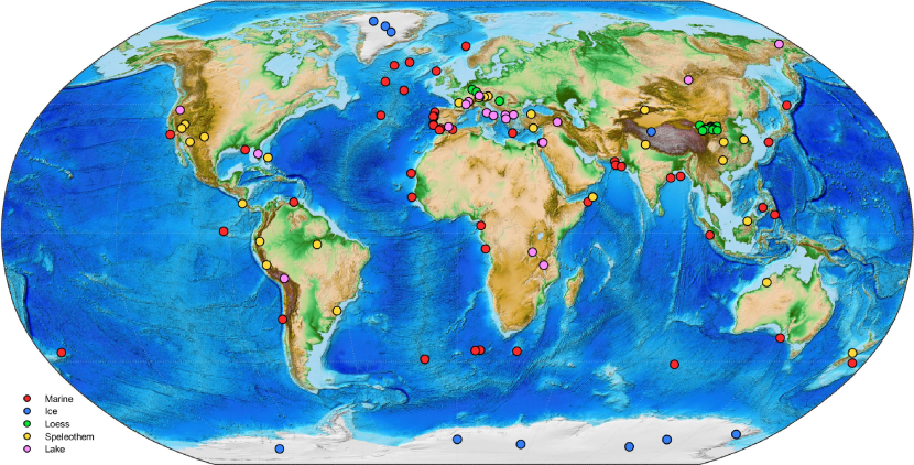
Figure 1: Map of records listed in the Supplementary Material (SM) and included in the PaleoJump database. The five record sources — marine sediments, ice cores, terrestrial deposits, speleothems, and lake sediments — are identified in the legend by color.

Applying the KS test and RQA to TP identification

Given the diversity of paleoclimate records, an objective, automated methodology is crucial for identifying and comparing TPs. Bagniewski et al. [13] have formulated an augmented KS test and applied it successfully to the robust detection and identification of abrupt transitions for the last glacial cycle. Their results were compared with RQA, showing the complementarity of the two methods, with KS more useful at detecting individual jumps and finding their precise dates, while RQA can help establish important transitions in a record’s characteristic time scale. Here we apply these two methods to selected records of the PaleoJump database and demonstrate the ability of the KS test to accurately identify transitions for different types of paleoclimate records.

Kolmogorov-Smirnov (KS) test.

The augmented KS methodology [13] is based on the nonparametric KS test [152]. A two-sample KS test is applied to two neighboring samples drawn from a proxy time series within a sliding window of length $w$. The commonality of the two samples is quantified by the the KS statistic $D_{\rm{KS}}$ [152, 153]. A “jump” in the time series is identified at any point in time at which $D_{\rm{KS}}$ is greater than a cut-off threshold $D_{\rm c}$. As the KS test can give very different results depending on the window length $w$ being used, $D_{\rm{KS}}$ is calculated for different $w$’s, varying between $w_{\rm{min}}$ and $w_{\rm{max}}$. The values of the latter two parameters bracket the desired time scale at which a given paleorecord is to be investigated. Furthermore, smaller jumps in the time series may be the result of an error in the observed data or small-scale variability that occurs over time intervals shorter than the sampling resolution of the proxy record and they should be discarded. Thus, for a transition to be considered significant, the change in magnitude between the two samples $(i,j)$ should exceed a threshold $\sigma_{\rm c}$ in their standard deviations $(\sigma_{i},\sigma_{j})$. Finally, as the KS test requires a large enough sample size to be significant, its results are rejected if either of the two samples has a size $n$ smaller than $n_{\rm c}$.

At a time step at which all three conditions based on the parameters $D_{\rm c}$, $\sigma_{\rm c}$, and $n_{\rm c}$ are satisfied, an abrupt transition is identified. As the dates of such transitions often occur in clusters, the precise date for a transition within such a cluster is determined by the maximum $D_{\rm{KS}}$ value found within the corresponding time interval. When the maximum $D_{\rm{KS}}$ over a given interval is shared by several time steps, the one corresponding to the maximum change in absolute magnitude is used; moreover, if there are several jumps of equal amplitude, then the one with the earliest date is used.

As the same transition may be found at slightly different dates depending on the window length that is used, we first identify the transitions detected with the longest window, which, given the larger sample size it accomodates, is the most statistically significant one. These transitions are then supplemented by those detected for the next-longest window and eventually for all other window lengths. For window $w_{i}$, we discard transitions identified at time $t$ if the interval $\{t-w_{i}\leq t\leq t+w_{i}\}$ contains transitions that were previously identified with a greater window length. Finally, long-term trends in maxima and minima are used to establish the main transitions, such as Stadial-Interstadial (GS – GI) boundaries.

The parameters $D_{\rm c}$ and $\sigma_{\rm c}$ are initially optimized following receiver operating characteristic analysis [154, 155], and abrupt transitions so identified for the NGRIP ice core $\delta^{18}$O record are further compared with the change points identified using visual inspection by Rasmussen et al. [88].

Recurrence Quantification Analysis (RQA).

The KS test results are next compared with RQA results [14, 15, 156]. Here, the Recurrence Plot (RP) for a time series $\{x_{k}:k=1,\ldots,K\}$ is given by a square pattern in which both axes represent time. A dot is entered into a position $(i,j)$ of the matrix $\mathbf{R}$ when $|x_{i}-x_{j}|<\varepsilon$, with $\varepsilon$ being the recurrence threshold. Thus, the RP appears as a square matrix $\mathbf{R}$ of dots. For details on how $\varepsilon$ is determined, see Marwan et al. [15] and Bagniewski et al. [13].

Eckmann et al. [14] showed that purely visual RP typologies provide useful information about a time series. However, RQA allows for a more objective way of inferring recurrence [15, 156], by quantifying selected recurrence characteristics. One of the simplest RQA criteria is the recurrence rate (RR), namely the density of dots within the recurrence plot: RR describes the probability of states of the system recurring within a particular time interval. By evaluating RQA measures such as RR in a sliding window, it is possible to identify changes in the time series. Low RR values correspond to an unstable behavior of the system, and hence abrupt transitions in a time series may be identified by local RR minima.

An important advantage of the recurrence method is that it does apply to dynamical systems that are not autonomous, i.e., that may be subject to time-dependent forcing [14]. The latter is certainly the case for the climate system in general [157, 158, 159, 160] and, in particular, on the time scales of 10–100 kyr and longer, which are affected strongly by orbital forcing [161].

For a more comprehensive description of both the augmented KS test and RQA, see Bagniewski et al. [13].

Examples of usage

Here we show the results of the augmented KS test methodology [13], as applied to records of different timescales, resolutions, and periodicities. Plots of the detected transitions, along with spreadsheets listing their dates are available on the PaleoJump database for other records as well.

Methodology.

To demonstrate the applicability of the PaleoJump database to the study of climate TPs, we tested herein the ability of the augmented KS test to detect abrupt transitions in different types of paleoproxy records. Specifically, we analyze six records, given in Table LABEL:tab:tableshort, from each of the proxy types listed in Supplementary Tables 1 – 5. In addition to these six records, we include the results obtained for the NGRIP ice core, which have been published in Bagniewski et al. [13], and compare the latter with the three records of the last climate cycle in the table, to wit MD03-2621, Paraiso Cave, and ODP893A.

Table 1: Records analyzed using the augmented KS test [13], ordered by geological type and temporal scale; the nature of the records is indicated by the abbreviations ben = benthic, pla = planktonic, and TIC = Total Inorganic Carbon in the last column.

Type	Site name	Location	Depth/elevation	Age	Res.	Proxy
Marine	ODP893A [37, 36]	34.28, -120.03	576 m	65 - 0 ka	41 y	pla $\delta^{18}$O
Marine	MD03-2621 [26]	10.678, -64.972	847 m	109 - 6 ka	0.1 y	reflectance
Marine	U1308 [44]	49.878, -24.238	3871 m	3143 - 0 ka	118 y	ben $\delta^{18}$O
Marine	CENOGRID [72]	N/A	N/A	67.1 - 0 Ma	2000 y	ben $\delta^{18}$O
Terrestrial	Paraiso (PAR07) [117]	-4.067, -55.45	60 m	45 - 18 ka	21 y	$\delta^{18}$O
Terrestrial	Lake Ohrid [146]	41.049, 20.715	693 m	1.36 - 0 Ma	208 y	TIC
Ice	NGRIP [88]	75.1, -42.32	2925 m	122 - 0 ka	20 y	$\delta^{18}$O

The KS test parameters vary depending on a record’s time resolution and on the length of its age interval. For the records covering the last climate cycle (MD03-2621, Paraiso Cave, and ODP893A), we use the same parameter values as used for the NGRIP record in Bagniewski et al. [13], i.e., $D_{\rm c}=0.77$, $\sigma_{\rm c}=1.9$, $n_{\rm c}=3$, $w_{\rm{min}}=0.1$ kyr, and $w_{\rm{max}}=2.5$ kyr. For the records spanning longer time intervals with a lower temporal resolution, we use longer window lengths $w_{\rm{min}}$ and $w_{\rm{max}}$, thus shifting the focus of our analysis to longer time scales. For the U1308 benthic $\delta^{18}$O and Lake Ohrid TIC records, we use a $w$-range of 2 kyr to 20 kyr. This allows us to focus on the glacial-cycle variability, as the record’s resolution is too low to properly identify DO events, particularly for data older than 1.5 Ma BP, when the U1308 record’s resolution is lower than for more recent data. For the CENOGRID record, we perform two separate analyses, one with a $w$-range of 1 Myr to 4 Myr to determine the Quaternary’s major climatic shifts, and one with a $w$-range of 0.02 Myr to 2.5 Myr, which covers the orbital time scale.

Results for Individual records.

We chose the MD03-2621 reflectance record from the Cariaco Basin in the Caribbean for having a very high resolution and for its importance in studying the effect of DO events on the migrations of the intertropical convergence zone (ITCZ). The record is shown in Fig. 2 and it has been used previously to assess teleconnections between the North Atlantic basin and the Arabian Sea [26]. When the ITCZ migrates southward during stadials, northeasterly Trade winds lead to upwelling of cool, nutrient-rich waters in the Caribbean; as the ITCZ migrates northward during interstadials, heavy convective rainfall leads to increased runoff from South America’s north coast, delivering detrital material to the Cariaco Basin [26, 162]. As a result, the color reflectance in the core alternates between light-colored sediments, rich in foraminiferal carbonate and silica, and darker sediments abundant in detrital organic carbon. These changes in the marine sediments are proxies for the prevailing atmospheric circulation regime, and the meridional position of the ITCZ in the region, which are both linked to the glacial-interglacial variability.

For the KS analysis, a 20-year moving average of the MD03-2621 record is calculated in order to align its resolution with that of the NGRIP record. Our analysis does identify the “classical” DO events, as seen in the NGRIP record [88, 13]. There is, however, no direct relationship in the identified longer-scale warm (grey bars) and cool intervals: For instance, some events appear to be merged in Fig. 2, e.g., GI 3 and 4, GI 9 and 10, GI 13 and 14, GI 15 and 16, and GI 22 and 23, while some events detected here, between 66 and 68 ka BP, are not identified in NGRIP, and GI 2 is much longer than in NGRIP.

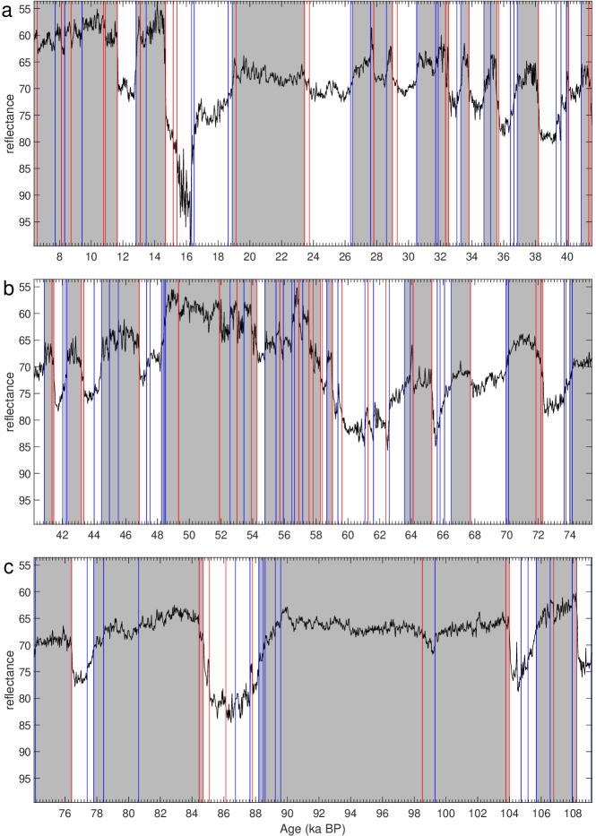
Figure 2: MD03-2621 marine sediment core. The black solid line is the core reflectance [26], with the vertical axis reversed. Vertical lines represent transitions detected by the KS test of Bagniewski et al. [13], with red lines for warming transitions, i.e., DO events, and blue lines for cooling ones. Grey bars represent warm episodes. Note that all time axes in this paper follow the geological custom of pointing into the past.

The RQA analysis [15, 156], shown in Fig. 3, does identify the major transitions in the MD03-2621 reflectance record, including the relative significance of each. It does not, however, resolve smaller transitions that occur at the centennial time scale. Please see Bagniewski et al. [13] for the explanation of the recurrence rate used to identify the transitions in the figure’s panel (c).

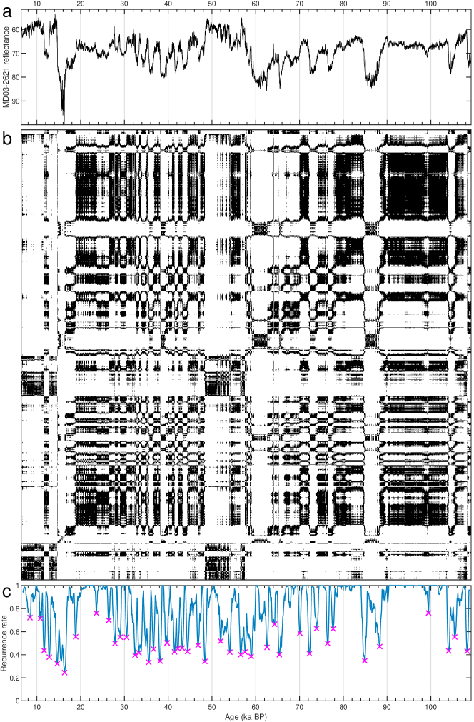
Figure 3: Recurrence Quantification Analysis (RQA)[15, 156] for the MD03-2621 reflectance record [26]. (a) Time series with vertical axis as in Fig. 2; (b) recurrence plot (RP); and (c) recurrence rate. Magenta crosses in panel (c) represent the transitions identified by the RQA.

The CENOGRID stack of benthic $\delta^{18}$O [72] shown here in Fig. 4 is a highly resolved 67 Myr composite from 14 marine records. Westerhold et al. [72] distinguished four climate states — Hothouse, Warmhouse, Coolhouse, and Icehouse — in this record, largely following changes in the polar ice volume. The composite in the figure [72] reconstructs in detail Earth’s climate during the Cenozoic era, at a higher time resolution than the earlier compilation of Zachos and colleagues [163].

Our KS analysis in Fig. 4a uses a window width $x\leq w\leq y$ and it identifies four major transitions towards higher $\delta^{18}$O values and two towards lower ones. The oldest threshold, at 58 Ma BP, characterizes the transition between the moderately warm climate prevailing at the beginning of the Cenozoic to the hot conditions marked by the Early Eocene Climate Optimum between 54 Ma and 49-48 Ma BP. The second transition corresponds to the short but intense warm event known as the PTEM, the Cenozoic’s hottest one. The third transition marks the end of this hot interval and the return to the milder and relatively stable conditions that prevailed between 67 Ma and 58 Ma BP.

The fourth threshold at 34 Ma is the Eocene–Oligocene Transition, the sharp boundary between the warm and the hot climatic conditions in the earlier Cenozoic and the Coolhouse and then Icehouse conditions prevailing later on[164]. This transition is an intriguing candidate for TP status in Earth’s climate history [165]. The fifth transition, at 14 Ma BP, ends a rather stable climate interval between 34 Ma and 14 Ma, characterized by the build up of the East Antarctic ice sheet[166, 167]. This transition also marks the start of an increasing trend in benthic $\delta^{18}$O values [168, 169]. The final transition marks the start of the Icehouse world and it is characterized by the emergence and development of the Northern Hemisphere ice sheets, with their further expansion occurring during the past 400 kyr; compare U1308 results in Fig. 7 below.

Using a reduced window length on the last 26 Myr of the CENOGRID benthic record, many more abrupt transitions are detected in Fig. 4b. In particular, higher variability in the $\delta^{18}$O signal and much more frequent transitions are found during two intervals, namely 71 transitions over the last 3.5 Myr and 77 transitions between 13 Ma BP and 20 Ma BP. In contrast, the intervals 3.5–13 Ma BP and 20–67 Ma BP are characterized by a lower frequency of detected transitions, with 13 and 112 transitions, respectively. The former one of the two intervals with many jumps includes the Quaternary Period, which started 2.6 Myr ago and is well known for its high climate variability, due to the presence of large ice masses in the system [170, 6].

The interval 13–20 Ma BP, on the other hand, coincides with the exclusive use of the U1337 and U1338 records in constructing the CENOGRID stack, both of which are located in the eastern tropical Pacific. Higher sedimentation rates in these two cores might contribute to the higher variability $\delta^{18}$O observed in the stack record over this interval. For transitions detected with the shorter window for the entire CENOGRID stack, please see Fig. S1 in the Supplementary Material.

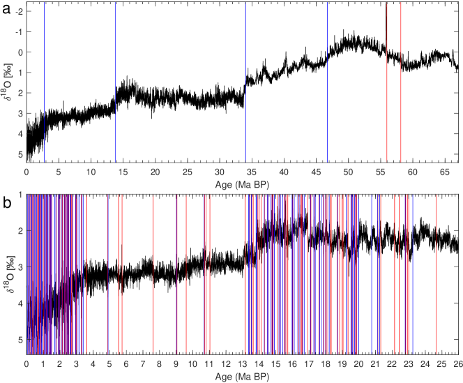
Figure 4: CENOGRID stack of benthic $\delta^{18}$O [72]. Vertical lines represent transitions detected by the KS test [13], with red lines for warming transitions and blue lines for cooling ones, while grey bars represent warm episodes. (a) Transitions detected for the entire record using a fixed window length of $w=5$ Myr, and (b) transitions detected for the interval 0–26 Ma BP using $0.01\leq w\leq 1.25$ Myr; see also the earlier subsection on “Methodology.” The vertical axes are reversed.

The $\delta^{18}$O record from the Paraiso Cave, located in the Amazon rainforest, shows moisture patterns that undergo abrupt shifts during DO events; see Fig. 5. It is likely that the Amazonian climate subsystem exhibits bistability, thus making it a potential tipping element, as changes in precipitation accelerate dieback of the forest[171]. The Paraiso Cave record indicates that rainfall over the Amazon basin corresponds to global temperature changes, with dryer conditions during the last glacial period. This record exhibits negative correlation with the Chinese speleothem records [100], suggesting that rainfall in these two regions is in phase opposition.

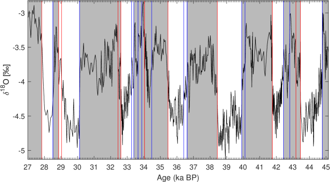
Figure 5: Paraiso Cave (PAR07) $\delta^{18}$O [117]. Vertical lines represent transitions detected by the KS algorithm [13], with red lines for a decrease in $\delta^{18}$O and blue lines for an increase in $\delta^{18}$O, while grey bars correspond to warm events.

Results for core intercomparisons.

In Fig. 6, we compare four paleorecords of different types and from distinct locations: NGRIP $\delta^{18}$O, MD03-2621 reflectance, Paraiso Cave $\delta^{18}$O, and ODP893A planktic $\delta^{18}$O from the Santa Barbara Basin. Overall, the abrupt transitions in the four records appear to be fairly synchronous, with the main Greenland DO events from NGRIP also observed for the two marine records and the one speleothem record. The transitions that correspond to Greenland interstadials (GIs) GI-3 to GI-12 [88] are identified in all four records, with only a few exceptions: GI-3 is not identified for the ODP893A record, due to an insufficient number of data points; and GI-5.1 is not identified in any record, except as a cooling event in MD03-2621 and in Paraiso cave. Also, GI-9 and GI-10 appear as a single interstadial in the Paraiso cave and ODP893A records, which is probably due to a decreased time resolution observed in both records during this time interval.

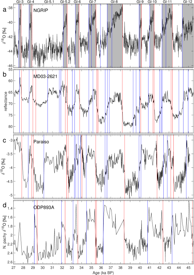
Figure 6: Comparison of four paleorecords over the 27 – 45.5 ka BP interval: (a) NGRIP ice core $\delta^{18}$O [88]; (b) MD03-2621 marine sediment reflectance [26]; (c) Paraiso Cave (PAR07) $\delta^{18}$O [117]; and (d) ODP893A marine sediment N. pachyderma $\delta^{18}$O [37, 36]. Vertical lines represent detected transitions, with red lines for warming transitions and blue lines for cooling ones. Grey bars in panel (a) represent interstadials identified for the NGRIP $\delta^{18}$O record, with top labels showing the Greenland Interstadials identified by Rasmussen et al. [88].

Finally, Fig. 7 shows the comparison between the U1308 benthic $\delta^{18}$O record and the Lake Ohrid Total Inorganic Carbon (TIC) record over a 1.4 Myr time interval that includes multiple glacial-interglacial transitions.

The U1308 benthic $\delta^{18}$O record in panel (a) of the figure is a 3.1 Myr record located within the ice-rafted detritus belt of the North Atlantic [172]. This record is a proxy for deep-water temperature and global ice volume, and it has enabled a detailed reconstruction of the history of orbital and millennial-scale climate variability during the Quaternary; it documents the changes in Northern Hemisphere ice sheets that follow the glacial–interglacial cycles [44, 173], as well as mode transitions identified at 2.55 Ma, 1.5 Ma, 1.25 Ma, 0.65 Ma and 0.35 Ma BP.

The 1.25–0.65 Ma BP interval in the figure corresponds to the Mid-Pleistocene Transition (MPT) interval with 1.25 Ma being followed by an increase in the amplitude of the glacial–interglacial fluctuations and a transition from a dominant periodicity near 40 kyr to one near 100 kyr; see Reichers et al. [161] and references therein. The most recent abrupt transition, at 0.35 Ma, leads to the strongest interglacial of the record, which corresponds to the marine isotope stage (MIS) 9. Here, our KS analysis agrees with the well established marine isotope stratigraphy of Lisiecki and Raymo [174] by detecting rapid warmings that correspond to the classical terminations leading to interglacials, as well as rapid coolings that initiate glacial stages.

The Lake Ohrid TIC record in Fig. 7b shows glacial–interglacial variability in biomass over the past 1.4 Myr. Here, our KS analysis shows numerous abrupt transitions towards high TIC intervals that correspond to interglacial episodes, as well as matching ones of opposite sign. The interglacial ones are associated with forested environmental conditions that are consistent with odd-numbered MISs, as was the case for the U1308 record in the figure’s panel (a). The glacial episodes, to the contrary, correspond to forestless conditions, that, according to the available timescale, are consistent with even-numbered MISs.

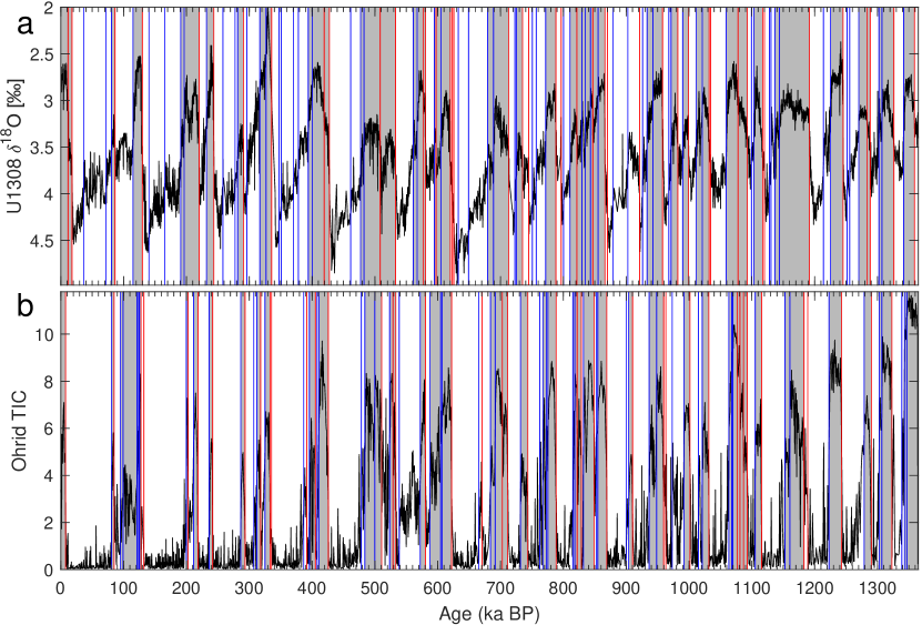
Figure 7: Comparison of the benthic Cibicidoides sp. $\delta^{18}$O record in (a) the U1308 marine-sediment core [44] and (b) Lake Ohrid TIC [146]. Vertical lines represent transitions detected by our KS methodology [13], with red lines for warming transitions and blue lines for cooling ones, while grey bars correspond to interglacials (odd-numbered MISs) and white bars correspond to glacials (even-numbered MISs).

Discussion

The two methods.

The augmented KS test of Bagniewski et al. [13] has detected abrupt transitions on different time scales in a variety of paleorecords. These include the NGRIP ice core, the Paraiso Cave speleothem, and the MD03-2621 and ODP893A marine sediment cores for the last climate cycle; the U1308 marine sediment core and Lake Ohrid TIC for the Middle and Late Pleistocene; and the CENOGRID marine sediment stack for the Cenozoic Era. While possible mechanisms giving rise to the observed variability in these records have been discussed in previous studies, the objective, precise and robust dating of the main transitions using the augmented KS test may allow a more detailed and definitive analysis and modelling.

The transitions identified with the RQA methodology [14, 15, 156] do correspond to a subset of those found with the KS test, but several smaller-scale transitions identified by the latter have not been found with the former method. The RQA approach, though, does allow one to quantify the magnitude of each transition, and it may thus be useful for identifying key transitions.

Interpretation of findings.

The high-resolution MD03-2621 reflectance record from the Cariaco Basin [26] in Fig. 2 shows abrupt transitions that are largely in agreement with those detected by our KS test for the NGRIP record. Desplazes et al. [26] have argued that these transitions are driven by the ITCZ displacements that occurred primarily in response to Northern Hemisphere temperature variations. These authors indicated that the ITCZ migrated seasonally during mild stadials, but was permanently displaced south of the Cariaco Basin during the colder stadial conditions. The very high resolution of the MD03-2621 record allows a detailed comparison with the transitions identified for the NGRIP record. The fact that several small-scale NGRIP transitions are not identified by our KS test in the MD03-2621 record suggests that a TP linked to ITCZ migration was not crossed during these events. Furthermore, the KS test does reveal transitions that have not been recognized previously in either record [88], e.g., at 86.15 ka BP, which we find in both the NGRIP and MD03-2621 records.

In the 67-Myr CENOGRID stack (Fig. 4) of benthic $\delta^{18}$O [72, 163], we identified four major cooling transitions that culminate with the start of the Pleistocene, as well as two warming transitions, including the Paleocene-Eocene Thermal Maximum. These major jumps agree with those identified in Westerhold et al. [72]. However, using a shorter window length, many more transitions were detected during the Pleistocene, well known for its higher climate variability [170, 6], as well as during the early Miocene, i.e., between the mid-Miocene transition at 14 Ma BP [167] and the Oligocene-Miocene transition at 23 Ma BP [175, 176, 177]. A possible reason is the fact that the 13–20 Ma BP interval in the stack has been constructed using records from the eastern Tropical Pacific. This region has been characterized by high upwelling rates and sedimentation rates in the past [178]. While the CENOGRID composite has a uniform resolution, higher sedimentation rates could affect the resolution of the original records and, therewith, even the variability seen in lower-resolution sampling. The fact that the source region of the data has a large effect on the frequency of detected transitions implies that caution is needed when using individual records as proxies for global climate.

The Paraiso Cave record [117] from the eastern Amazon lowlands in Fig. 5 shows dryer conditions during the last glacial period, with abrupt transitions matching those that correspond to the DO events identified in the NGRIP ice core record. The Amazon record is also in fairly good agreement with the nearby MD03-2621 marine sediment record. Notably, several of NGRIP’s DO events appear combined in both records, namely GI-5.1 and GI-5.2, as well as GI-9 and GI-10, which might indicate that a climate change event over Greenland did not trigger a tipping event in the Amazon basin. Alternatively, the first merging may question the separation of the classical GI-5 event [179] into two distinct events, 5.1 and 5.2.

The comparison of four records on the same time scale in Fig. 6 demonstrates that a signal of abrupt climate change is detected when using the KS method with similar accuracy for different types of paleodata. The differences in the dates of the transitions may be largely explained by the use of different age models in each of the records, with MD03-2621 fine-tuned to the NGRIP chronology, and ODP893A fine-tuned to the GISP2 chronology, while the NGRIP and Paraiso Cave records were independently dated. Notably, ODP893A data prior to GI-8 appear misaligned with the other three records. The chronology of jumps in ODP893A indicates that the warm interval between 40.8 ka BP and 42.4 ka BP may correspond to an event spanning GI-9 and GI-10, while the warm interval between 43.3 ka BP and 45.3 ka BP may correspond to GI-11.

In addition to the classical GI transitions, several additional jumps are identified in each of the marine and cave records. These jumps may be the representative of local climate changes or, in some cases, be artifacts of sampling resolution or measurement error. Stronger evidence for a local or regional event may be obtained when comparing two nearby records, like the Paraiso Cave in the Amazon and the MD03-2621 marine record from the Cariaco Basin. In both records, the start of GI-5.2 is represented as two warming transitions, in contrast with the NGRIP and ODP893A records, where only one sharp transition is present. Likewise, the end of GI-9 in the two tropical, South American records appears as two successive cooling events. These results point to the potential of using the KS method to improve fine-tuning the synchroneity of two or more records, when an independent dating method is not available.

The comparison in Fig. 7 of KS-detected transitions in marine core U1308 [44] and in Lake Ohrid TIC [146] identifies the transitions between individual glacials and interglacials. In the two records, the transitions are well identified, despite the resolution of the two being different, and they offer a precise dating for the chronology of the past glacial cycles. The transitions are overall in good agreement between the two records. Still, the warm events in Lake Ohrid are essentially atmospheric and thus have often a shorter duration than in the marine record, while cooling transitions precede those in the deep ocean by several thousand years. This could indicate that a significant time lag is present, either in ice sheet growth in response to atmospheric cooling, or in the propagation of the cooling signal into the deep North Atlantic.

Furthermore, there are atmospheric interglacial episodes missing in the oceanic U1308 record. This mismatch between the lake record [146] and the marine one [44] could be attributed to the fact that the KS test does sometimes find more transitions in one record than in another one, even for the same type of proxy and within the same region. Such occurrences may be due to the local environment, the sampling method, or some aspect of the KS method itself. When this is the case, it is important — although not always feasible — to find one or more additional records covering a similar time interval with a similar resolution, in order to shed further light on the mismatch between the two original records.

Concluding remarks

The carefully selected, high-quality paleoproxy records in the PaleoJump database [12], https://paleojump.github.io, have different temporal scales and a global spatial coverage; see again Fig. 1. These records provide an easily accessible resource for research on potential tipping elements in Earth’s climate. Still, major gaps in the marine sediment records exist in the Southern Hemisphere, especially in the Indian and Pacific Oceans. Only sparse terrestrial data are available from the high latitudes in both hemispheres, due to the recent glaciation. The only data from the African continent come from two East African lake sediment records. Even though much information is at hand from the more than 100 sites listed in this paper, more records are needed to fill geographical and temporal gaps, especially in the Southern Hemisphere.

The examples given in the paper on abrupt-transition identification demonstrate the usefulness of the records included in PaleoJump for learning about potential tipping events in Earth’s history and for comparing such events across different locations around the world. The accessibility of such high-quality records is an invaluable resource for the climate modelling community that requires comparing their results across a hierarchy of models [160, 180] with observations.

We also demonstrated the usefulness of the KS test [13] for establishing precisely the chronology of Earth’s main climatic events. The newly developed tool for automatic detection of abrupt transitions may be applied to different types of paleorecords, allowing to objectively and robustly characterize the tipping phenomenon for climate subsystems already suspected of being subject to tipping [9], but also to identify previously unrecognized tipping elements in past climates. The observational descriptions of tipping that can be obtained from PaleoJump using our KS methodology, combined with the application of Earth System Models, can help improve the understanding of the bifurcation mechanisms of global and regional climate and identify possible TPs for future climates.

Our results also indicate that paleorecord interpretations may vary, since the abrupt transitions identified in them will depend on the time scale and type of variability that is investigated. For example, the KS method’s parameters [13] may be changed when studying different proxy record resolutions, affecting the frequency and exact timing of the TPs that are identified.

The agreement in timing and pattern between jumps in distinct records can confirm the correctness of each record separately, as well as of the inferences on climate variability drawn from these jumps. Specifically, the ability of the KS method to identify matching small-scale transitions in different high-resolution records may be used to validate these transitions as being the result of genuine global or regional climatic events, as opposed to just sampling errors. Furthermore, significant differences in records that are, overall, in good agreement with each other may help decode the chronology of tipping events or an approximate range for a tipping threshold. A fortiori, the differences in timing and pattern between jumps in distinct records that we also found emphasize the importance of a consistent dating methodology.

The broad spatial coverage of the PaleoJump database [12], https://paleojump.github.io, with its records that vary in their nature — ice, marine and land — as well as in their length and resolution, will facilitate research on tipping elements in Earth’s climate, including the polar ice sheets, the Atlantic Meridional Overturning Circulation, and the tropical rainforests and monsoon systems. Furthermore, it will support establishing improved criteria on where and how to collect data for reliable early warning signals of impending TPs.

Author contributions statement

W.B., M.G. and D.D.R. outlined the manuscript, W.B. carried out the computations and drew the plots, and W.B., M.G. and D.D.R. analyzed the results. W.B. drafted the manuscript and all authors reviewed and finalized it.

Competing interests

The authors declare no competing interests.

References

- [1] Dansgaard, W. et al. A new Greenland deep ice core. Science 218, 1273–1277 (1982).
- [2] Johnsen, S. et al. Irregular glacial interstadials recorded in a new Greenland ice core. Nature 359, 311–313 (1992).
- [3] Grootes, P. M., Stuiver, M., White, J., Johnsen, S. & Jouzel, J. Comparison of oxygen isotope records from the GISP2 and GRIP Greenland ice cores. Nature 366, 552–554 (1993).
- [4] Shackleton, N. J., Hall, M. A. & Vincent, E. Phase relationships between millennial-scale events 64,000–24,000 years ago. Paleoceanography 15, 565–569 (2000).
- [5] Genty, D. et al. Precise dating of Dansgaard–Oeschger climate oscillations in western Europe from stalagmite data. Nature 421, 833–837 (2003).
- [6] Ghil, M. & Childress, S. Topics in Geophysical Fluid Dynamics: Atmospheric Dynamics, Dynamo Theory, and Climate Dynamics (Springer Science+Business Media, Berlin/Heidelberg, 1987). Reissued as an eBook in 2012.
- [7] Ghil, M. & Lucarini, V. The physics of climate variability and climate change. Reviews of Modern Physics 92, 035002 (2020).
- [8] Pearce, F. With Speed and Violence: Why Scientists Fear Tipping Points in Climate Change (Beacon Press, 2007).
- [9] Lenton, T. M. et al. Tipping elements in the Earth’s climate system. Proceedings of the national Academy of Sciences 105, 1786–1793 (2008).
- [10] Scheffer, M. et al. Early-warning signals for critical transitions. Nature 461, 53–59 (2009).
- [11] Wunderling, N., Donges, J. F., Kurths, J. & Winkelmann, R. Interacting tipping elements increase risk of climate domino effects under global warming. Earth System Dynamics 12, 601–619 (2021).
- [12] Bagniewski, W., Rousseau, D.-D. & Ghil, M. Paleojump (2022). URL https://doi.org/10.5281/zenodo.6534031.
- [13] Bagniewski, W., Ghil, M. & Rousseau, D.-D. Automatic detection of abrupt transitions in paleoclimate records. Chaos 31, 113129 (2021).
- [14] Eckmann, J.-P., Kamphorst, S. O. & Ruelle, D. Recurrence plots of dynamical systems. Europhysics Letters 4, 973–977 (1987).
- [15] Marwan, N., Romano, M. C., Thiel, M. & Kurths, J. Recurrence plots for the analysis of complex systems. Physics reports 438, 237–329 (2007).
- [16] Bahr, A. et al. Oceanic heat pulses fueling moisture transport towards continental Europe across the mid-Pleistocene transition. Quaternary Science Reviews 179, 48–58 (2018).
- [17] Barker, S. & Diz, P. Timing of the descent into the last Ice Age determined by the bipolar seesaw. Paleoceanography 29, 489–507 (2014).
- [18] Barker, S. et al. Early interglacial legacy of deglacial climate instability. Paleoceanography and Paleoclimatology 34, 1455–1475 (2019).
- [19] Beuscher, S. et al. End-member modelling as a tool for climate reconstruction—an Eastern Mediterranean case study. Plos one 12, e0185136 (2017).
- [20] Bolton, C. T. et al. North Atlantic midlatitude surface-circulation changes through the Plio-Pleistocene intensification of Northern Hemisphere glaciation. Paleoceanography and Paleoclimatology 33, 1186–1205 (2018).
- [21] Clemens, S. et al. Precession-band variance missing from East Asian monsoon runoff. Nature communications 9, 1–12 (2018).
- [22] Clemens, S. C. et al. Remote and local drivers of Pleistocene South Asian summer monsoon precipitation: A test for future predictions. Science Advances 7, eabg3848 (2021).
- [23] Davtian, N., Bard, E., Darfeuil, S., Ménot, G. & Rostek, F. The Novel Hydroxylated Tetraether Index RI-OH’ as a Sea Surface Temperature Proxy for the 160-45 ka BP Period Off the Iberian Margin. Paleoceanography and Paleoclimatology 36, e2020PA004077 (2021).
- [24] de Abreu, L., Shackleton, N. J., Schönfeld, J., Hall, M. & Chapman, M. Millennial-scale oceanic climate variability off the Western Iberian margin during the last two glacial periods. Marine Geology 196, 1–20 (2003).
- [25] De Deckker, P. et al. Climatic evolution in the Australian region over the last 94 ka-spanning human occupancy-, and unveiling the Last Glacial Maximum. Quaternary Science Reviews 249, 106593 (2020).
- [26] Deplazes, G. et al. Links between tropical rainfall and North Atlantic climate during the last glacial period. Nature Geoscience 6, 213–217 (2013).
- [27] Deplazes, G. et al. Weakening and strengthening of the Indian monsoon during Heinrich events and Dansgaard-Oeschger oscillations. Paleoceanography 29, 99–114 (2014).
- [28] De Pol-Holz, R. et al. Late Quaternary variability of sedimentary nitrogen isotopes in the eastern South Pacific Ocean. Paleoceanography 22 (2007).
- [29] Dickson, A. J., Austin, W. E., Hall, I. R., Maslin, M. A. & Kucera, M. Centennial-scale evolution of Dansgaard-Oeschger events in the northeast Atlantic Ocean between 39.5 and 56.5 ka BP. Paleoceanography 23 (2008).
- [30] Dokken, T. M. & Jansen, E. Rapid changes in the mechanism of ocean convection during the last glacial period. Nature 401, 458–461 (1999).
- [31] Ehrmann, W. & Schmiedl, G. Nature and dynamics of North African humid and dry periods during the last 200,000 years documented in the clay fraction of Eastern Mediterranean deep-sea sediments. Quaternary Science Reviews 260, 106925 (2021).
- [32] Elderfield, H. et al. Evolution of ocean temperature and ice volume through the mid-Pleistocene climate transition. Science 337, 704–709 (2012).
- [33] Eynaud, F. et al. Position of the Polar Front along the western Iberian margin during key cold episodes of the last 45 ka. Geochemistry, Geophysics, Geosystems 10 (2009).
- [34] Gottschalk, J., Skinner, L. C. & Waelbroeck, C. Contribution of seasonal sub-Antarctic surface water variability to millennial-scale changes in atmospheric CO2 over the last deglaciation and Marine Isotope Stage 3. Earth and planetary science letters 411, 87–99 (2015).
- [35] Harada, N. et al. Rapid fluctuation of alkenone temperature in the southwestern Okhotsk Sea during the past 120 ky. Global and Planetary Change 53, 29–46 (2006).
- [36] Hendy, I. L. & Kennett, J. P. Latest Quaternary North Pacific surface-water responses imply atmosphere-driven climate instability. Geology 27, 291–294 (1999).
- [37] Hendy, I. L., Kennett, J. P., Roark, E. & Ingram, B. L. Apparent synchroneity of submillennial scale climate events between Greenland and Santa Barbara Basin, California from 30–10 ka. Quaternary Science Reviews 21, 1167–1184 (2002).
- [38] Hendy, I. L. & Kennett, J. P. Tropical forcing of North Pacific intermediate water distribution during Late Quaternary rapid climate change? Quaternary Science Reviews 22, 673–689 (2003).
- [39] Hodell, D. A., Venz, K. A., Charles, C. D. & Ninnemann, U. S. Pleistocene vertical carbon isotope and carbonate gradients in the South Atlantic sector of the Southern Ocean. Geochemistry, Geophysics, Geosystems 4, 1–19 (2003).
- [40] Hodell, D. A., Channell, J. E., Curtis, J. H., Romero, O. E. & Röhl, U. Onset of “Hudson Strait” Heinrich events in the eastern North Atlantic at the end of the middle Pleistocene transition ( 640 ka)? Paleoceanography 23 (2008).
- [41] Hodell, D. A., Evans, H. F., Channell, J. E. & Curtis, J. H. Phase relationships of North Atlantic ice-rafted debris and surface-deep climate proxies during the last glacial period. Quaternary Science Reviews 29, 3875–3886 (2010).
- [42] Hodell, D. et al. Response of Iberian Margin sediments to orbital and suborbital forcing over the past 420 ka. Paleoceanography 28, 185–199 (2013).
- [43] Hodell, D. et al. A reference time scale for Site U1385 (Shackleton Site) on the SW Iberian Margin. Global and Planetary Change 133, 49–64 (2015).
- [44] Hodell, D. A. & Channell, J. E. Mode transitions in Northern Hemisphere glaciation: co-evolution of millennial and orbital variability in Quaternary climate. Climate of the Past 12, 1805–1828 (2016).
- [45] Jung, S. J., Kroon, D., Ganssen, G., Peeters, F. & Ganeshram, R. Enhanced Arabian Sea intermediate water flow during glacial North Atlantic cold phases. Earth and Planetary Science Letters 280, 220–228 (2009).
- [46] Lauterbach, S. et al. An ~130 kyr record of surface water temperature and 18O from the northern Bay of Bengal: Investigating the linkage between Heinrich events and Weak Monsoon Intervals in Asia. Paleoceanography and Paleoclimatology 35, e2019PA003646 (2020).
- [47] Lea, D. W. et al. Paleoclimate history of Galápagos surface waters over the last 135,000 yr. Quaternary Science Reviews 25, 1152–1167 (2006).
- [48] Martrat, B. et al. Four climate cycles of recurring deep and surface water destabilizations on the Iberian margin. Science 317, 502–507 (2007).
- [49] Mohtadi, M. et al. North Atlantic forcing of tropical Indian Ocean climate. Nature 509, 76–80 (2014).
- [50] Naafs, B., Hefter, J. & Stein, R. Millennial-scale ice rafting events and Hudson Strait Heinrich (-like) Events during the late Pliocene and Pleistocene: a review. Quaternary Science Reviews 80, 1–28 (2013).
- [51] Naafs, B. D. A., Voelker, A., Karas, C., Andersen, N. & Sierro, F. Repeated near-collapse of the Pliocene sea surface temperature gradient in the North Atlantic. Paleoceanography and Paleoclimatology 35, e2020PA003905 (2020).
- [52] Naughton, F. et al. Wet to dry climatic trend in north-western Iberia within Heinrich events. Earth and Planetary Science Letters 284, 329–342 (2009).
- [53] Nürnberg, D., Ziegler, M., Karas, C., Tiedemann, R. & Schmidt, M. W. Interacting Loop Current variability and Mississippi River discharge over the past 400 kyr. Earth and Planetary Science Letters 272, 278–289 (2008).
- [54] Pahnke, K., Zahn, R., Elderfield, H. & Schulz, M. 340,000-year centennial-scale marine record of Southern Hemisphere climatic oscillation. Science 301, 948–952 (2003).
- [55] Pichevin, L., Bard, E., Martinez, P. & Billy, I. Evidence of ventilation changes in the Arabian Sea during the late Quaternary: Implication for denitrification and nitrous oxide emission. Global Biogeochemical Cycles 21 (2007).
- [56] Rampen, S. W. et al. Long chain 1, 13-and 1, 15-diols as a potential proxy for palaeotemperature reconstruction. Geochimica et Cosmochimica Acta 84, 204–216 (2012).
- [57] Rickaby, R. E. M. & Elderfield, H. Planktonic foraminiferal Cd/Ca: paleonutrients or paleotemperature? Paleoceanography 14, 293–303 (1999).
- [58] Riveiros, N. V. et al. Response of South Atlantic deep waters to deglacial warming during Terminations V and I. Earth and Planetary Science Letters 298, 323–333 (2010).
- [59] Rosenthal, Y., Oppo, D. W. & Linsley, B. K. The amplitude and phasing of climate change during the last deglaciation in the Sulu Sea, western equatorial Pacific. Geophysical Research Letters 30 (2003).
- [60] Saikku, R., Stott, L. & Thunell, R. A bi-polar signal recorded in the western tropical Pacific: Northern and Southern Hemisphere climate records from the Pacific warm pool during the last Ice Age. Quaternary Science Reviews 28, 2374–2385 (2009).
- [61] Salgueiro, E. et al. Past circulation along the western Iberian margin: a time slice vision from the Last Glacial to the Holocene. Quaternary Science Reviews 106, 316–329 (2014).
- [62] Sánchez Goñi, M. F. et al. The ACER pollen and charcoal database: a global resource to document vegetation and fire response to abrupt climate changes during the last glacial period. Earth System Science Data 9, 679–695 (2017).
- [63] Schulz, H., von Rad, U. & Erlenkeuser, H. Correlation between Arabian Sea and Greenland climate oscillations of the past 110,000 years. Nature 393, 54–57 (1998).
- [64] Stott, L., Poulsen, C., Lund, S. & Thunell, R. Super ENSO and global climate oscillations at millennial time scales. science 297, 222–226 (2002).
- [65] Van Kreveld, S. et al. Potential links between surging ice sheets, circulation changes, and the Dansgaard-Oeschger cycles in the Irminger Sea, 60–18 kyr. Paleoceanography 15, 425–442 (2000).
- [66] Voelker, A. H. et al. Mediterranean outflow strengthening during northern hemisphere coolings: a salt source for the glacial Atlantic? Earth and Planetary Science Letters 245, 39–55 (2006).
- [67] Voelker, A. H. & Abreu, L. d. A review of abrupt climate change events in the Northeastern Atlantic Ocean (Iberian Margin): latitudinal, longitudinal and vertical gradients. AGU Geophysical Monograph (2010).
- [68] Waelbroeck, C. et al. Consistently dated Atlantic sediment cores over the last 40 thousand years. Scientific data 6, 1–12 (2019).
- [69] Weijers, J. W., Schouten, S., Schefuß, E., Schneider, R. R. & Damste, J. S. S. Disentangling marine, soil and plant organic carbon contributions to continental margin sediments: a multi-proxy approach in a 20,000 year sediment record from the Congo deep-sea fan. Geochimica et Cosmochimica Acta 73, 119–132 (2009).
- [70] Weldeab, S., Emeis, K.-C., Hemleben, C., Schmiedl, G. & Schulz, H. Spatial productivity variations during formation of sapropels S5 and S6 in the Mediterranean Sea: evidence from Ba contents. Palaeogeography, Palaeoclimatology, Palaeoecology 191, 169–190 (2003).
- [71] Weldeab, S., Lea, D. W., Schneider, R. R. & Andersen, N. 155,000 years of West African monsoon and ocean thermal evolution. science 316, 1303–1307 (2007).
- [72] Westerhold, T. et al. An astronomically dated record of Earth’s climate and its predictability over the last 66 million years. Science 369, 1383–1387 (2020).
- [73] Zarriess, M. & Mackensen, A. The tropical rainbelt and productivity changes off northwest Africa: A 31,000-year high-resolution record. Marine Micropaleontology 76, 76–91 (2010).
- [74] Zhao, M., Beveridge, N., Shackleton, N., Sarnthein, M. & Eglinton, G. Molecular stratigraphy of cores off northwest Africa: Sea surface temperature history over the last 80 ka. Paleoceanography 10, 661–675 (1995).
- [75] Ziegler, M., Diz, P., Hall, I. R. & Zahn, R. Millennial-scale changes in atmospheric CO 2 levels linked to the Southern Ocean carbon isotope gradient and dust flux. Nature Geoscience 6, 457–461 (2013).
- [76] Barbante, C. et al. One-to-one coupling of glacial climate variability in Greenland and Antarctica. Nature 444, 195–198 (2006).
- [77] Barker, S. et al. 800,000 years of abrupt climate variability. science 334, 347–351 (2011).
- [78] Baumgartner, M. et al. NGRIP CH 4 concentration from 120 to 10 kyr before present and its relation to a 15 N temperature reconstruction from the same ice core. Climate of the Past 10, 903–920 (2014).
- [79] Bazin, L. et al. An optimized multi-proxy, multi-site Antarctic ice and gas orbital chronology (AICC2012): 120–800 ka. Climate of the Past 9, 1715–1731 (2013).
- [80] Extier, T. et al. On the use of 18Oatm for ice core dating. Quaternary science reviews 185, 244–257 (2018).
- [81] Jouzel, J. et al. Orbital and millennial Antarctic climate variability over the past 800,000 years. science 317, 793–796 (2007).
- [82] Lambert, F. et al. Dust-climate couplings over the past 800,000 years from the EPICA Dome C ice core. Nature 452, 616–619 (2008).
- [83] Lambert, F., Bigler, M., Steffensen, J. P., Hutterli, M. & Fischer, H. Centennial mineral dust variability in high-resolution ice core data from Dome C, Antarctica. Climate of the Past 8, 609–623 (2012).
- [84] Loulergue, L. et al. Orbital and millennial-scale features of atmospheric CH4 over the past 800,000 years. Nature 453, 383–386 (2008).
- [85] Lüthi, D. et al. High-resolution carbon dioxide concentration record 650,000–800,000 years before present. Nature 453, 379–382 (2008).
- [86] Petit, J.-R. et al. Climate and atmospheric history of the past 420,000 years from the Vostok ice core, Antarctica. Nature 399, 429–436 (1999).
- [87] Rasmussen, S. O. et al. A first chronology for the North Greenland Eemian Ice Drilling (NEEM) ice core. Climate of the Past 9, 2713–2730 (2013).
- [88] Rasmussen, S. O. et al. A stratigraphic framework for abrupt climatic changes during the Last Glacial period based on three synchronized Greenland ice-core records: refining and extending the INTIMATE event stratigraphy. Quaternary Science Reviews 106, 14–28 (2014).
- [89] Thompson, L. G. et al. Tropical climate instability: The last glacial cycle from a Qinghai-Tibetan ice core. science 276, 1821–1825 (1997).
- [90] Vallelonga, P. et al. Iron fluxes to Talos Dome, Antarctica, over the past 200 kyr. Climate of the Past 9, 597–604 (2013).
- [91] Uemura, R. et al. Asynchrony between Antarctic temperature and CO2 associated with obliquity over the past 720,000 years. Nature communications 9, 1–11 (2018).
- [92] WAIS Divide Project Members. Precise interpolar phasing of abrupt climate change during the last ice age. Nature 520, 661–665 (2015).
- [93] Arienzo, M. M. et al. Bahamian speleothem reveals temperature decrease associated with Heinrich stadials. Earth and Planetary Science Letters 430, 377–386 (2015).
- [94] Asmerom, Y., Polyak, V. J. & Burns, S. J. Variable winter moisture in the southwestern United States linked to rapid glacial climate shifts. Nature Geoscience 3, 114–117 (2010).
- [95] Bar-Matthews, M., Ayalon, A., Gilmour, M., Matthews, A. & Hawkesworth, C. J. Sea–land oxygen isotopic relationships from planktonic foraminifera and speleothems in the Eastern Mediterranean region and their implication for paleorainfall during interglacial intervals. Geochimica et Cosmochimica Acta 67, 3181–3199 (2003).
- [96] Boch, R. et al. NALPS: a precisely dated European climate record 120–60 ka. Climate of the Past 7, 1247–1259 (2011).
- [97] Burns, S. J., Fleitmann, D., Matter, A., Kramers, J. & Al-Subbary, A. A. Indian Ocean climate and an absolute chronology over Dansgaard/Oeschger events 9 to 13. Science 301, 1365–1367 (2003).
- [98] Carolin, S. A. et al. Varied response of western Pacific hydrology to climate forcings over the last glacial period. Science 340, 1564–1566 (2013).
- [99] Cheng, H. et al. The climatic cyclicity in semiarid-arid central Asia over the past 500,000 years. Geophysical Research Letters 39 (2012).
- [100] Cheng, H. et al. The Asian monsoon over the past 640,000 years and ice age terminations. Nature 534, 640–646 (2016).
- [101] Cruz, F. W. et al. Insolation-driven changes in atmospheric circulation over the past 116,000 years in subtropical Brazil. Nature 434, 63–66 (2005).
- [102] Denniston, R. F. et al. North Atlantic forcing of millennial-scale Indo-Australian monsoon dynamics during the Last Glacial period. Quaternary Science Reviews 72, 159–168 (2013).
- [103] Fleitmann, D. et al. Timing and climatic impact of Greenland interstadials recorded in stalagmites from northern Turkey. Geophysical Research Letters 36 (2009).
- [104] Genty, D. et al. Isotopic characterization of rapid climatic events during OIS3 and OIS4 in Villars Cave stalagmites (SW-France) and correlation with Atlantic and Mediterranean pollen records. Quaternary Science Reviews 29, 2799–2820 (2010).
- [105] Kanner, L. C., Burns, S. J., Cheng, H. & Edwards, R. L. High-latitude forcing of the South American summer monsoon during the last glacial. Science 335, 570–573 (2012).
- [106] Kathayat, G. et al. Indian monsoon variability on millennial-orbital timescales. Scientific Reports 6, 1–7 (2016).
- [107] Kelly, M. J. et al. High resolution characterization of the Asian Monsoon between 146,000 and 99,000 years BP from Dongge Cave, China and global correlation of events surrounding Termination II. Palaeogeography, Palaeoclimatology, Palaeoecology 236, 20–38 (2006).
- [108] Lachniet, M. S. et al. Late Quaternary moisture export across Central America and to Greenland: evidence for tropical rainfall variability from Costa Rican stalagmites. Quaternary Science Reviews 28, 3348–3360 (2009).
- [109] Lachniet, M. S., Denniston, R. F., Asmerom, Y. & Polyak, V. J. Orbital control of western North America atmospheric circulation and climate over two glacial cycles. Nature communications 5, 1–8 (2014).
- [110] Mosblech, N. A. et al. North Atlantic forcing of Amazonian precipitation during the last ice age. Nature Geoscience 5, 817–820 (2012).
- [111] Moseley, G. E. et al. Reconciliation of the Devils Hole climate record with orbital forcing. Science 351, 165–168 (2016).
- [112] Moseley, G. E. et al. NALPS19: sub-orbital-scale climate variability recorded in northern Alpine speleothems during the last glacial period. Climate of the Past 16, 29–50 (2020).
- [113] Ünal-İmer, E. et al. An 80 kyr-long continuous speleothem record from Dim Cave, SW Turkey with paleoclimatic implications for the Eastern Mediterranean. Scientific reports 5, 1–11 (2015).
- [114] Wagner, J. D. et al. Moisture variability in the southwestern United States linked to abrupt glacial climate change. Nature Geoscience 3, 110–113 (2010).
- [115] Wang, Y.-J. et al. A high-resolution absolute-dated late Pleistocene monsoon record from Hulu Cave, China. Science 294, 2345–2348 (2001).
- [116] Wang, Y. et al. Millennial-and orbital-scale changes in the East Asian monsoon over the past 224,000 years. Nature 451, 1090–1093 (2008).
- [117] Wang, X. et al. Hydroclimate changes across the Amazon lowlands over the past 45,000 years. Nature 541, 204–207 (2017).
- [118] Whittaker, T. E., Hendy, C. H. & Hellstrom, J. C. Abrupt millennial-scale changes in intensity of Southern Hemisphere westerly winds during marine isotope stages 2–4. Geology 39, 455–458 (2011).
- [119] Hao, Q. et al. Delayed build-up of Arctic ice sheets during 400,000-year minima in insolation variability. Nature 490, 393–396 (2012).
- [120] Moine, O. et al. The impact of Last Glacial climate variability in west-European loess revealed by radiocarbon dating of fossil earthworm granules. Proceedings of the National Academy of Sciences 114, 6209–6214 (2017).
- [121] Seelos, K., Sirocko, F. & Dietrich, S. A continuous high-resolution dust record for the reconstruction of wind systems in central Europe (Eifel, Western Germany) over the past 133 ka. Geophysical Research Letters 36 (2009).
- [122] Sun, Y., Wang, X., Liu, Q. & Clemens, S. C. Impacts of post-depositional processes on rapid monsoon signals recorded by the last glacial loess deposits of northern China. Earth and Planetary Science Letters 289, 171–179 (2010).
- [123] Sun, Y. et al. Influence of Atlantic meridional overturning circulation on the East Asian winter monsoon. Nature Geoscience 5, 46–49 (2012).
- [124] Rousseau, D.-D. et al. (MIS3 & 2) millennial oscillations in Greenland dust and Eurasian aeolian records–A paleosol perspective. Quaternary Science Reviews 169, 99–113 (2017).
- [125] Újvári, G. et al. AMS 14C and OSL/IRSL dating of the Dunaszekcső loess sequence (Hungary): chronology for 20 to 150 ka and implications for establishing reliable age–depth models for the last 40 ka. Quaternary Science Reviews 106, 140–154 (2014).
- [126] Yang, S. & Ding, Z. A 249 kyr stack of eight loess grain size records from northern China documenting millennial-scale climate variability. Geochemistry, Geophysics, Geosystems 15, 798–814 (2014).
- [127] Allen, J. R. et al. Rapid environmental changes in southern Europe during the last glacial period. Nature 400, 740–743 (1999).
- [128] Allen, J. R., Watts, W. A. & Huntley, B. Weichselian palynostratigraphy, palaeovegetation and palaeoenvironment; the record from Lago Grande di Monticchio, southern Italy. Quaternary International 73, 91–110 (2000).
- [129] Ampel, L., Wohlfarth, B., Risberg, J. & Veres, D. Paleolimnological response to millennial and centennial scale climate variability during MIS 3 and 2 as suggested by the diatom record in Les Echets, France. Quaternary Science Reviews 27, 1493–1504 (2008).
- [130] Benson, L., Lund, S., Negrini, R., Linsley, B. & Zic, M. Response of north American Great basin lakes to Dansgaard–Oeschger oscillations. Quaternary Science Reviews 22, 2239–2251 (2003).
- [131] Camuera, J. et al. Orbital-scale environmental and climatic changes recorded in a new 200,000-year-long multiproxy sedimentary record from Padul, southern Iberian Peninsula. Quaternary Science Reviews 198, 91–114 (2018).
- [132] Donders, T. et al. 1.36 million years of Mediterranean forest refugium dynamics in response to glacial–interglacial cycle strength. Proceedings of the National Academy of Sciences 118 (2021).
- [133] Follieri, M., Magri, D. & Sadori, L. Pollen stratigraphical synthesis from Valle di Castiglione (Roma). Quaternary International 3, 81–84 (1989).
- [134] Fritz, S. C. et al. Quaternary glaciation and hydrologic variation in the South American tropics as reconstructed from the Lake Titicaca drilling project. Quaternary Research 68, 410–420 (2007).
- [135] Fritz, S. C., Baker, P., Ekdahl, E., Seltzer, G. & Stevens, L. Millennial-scale climate variability during the Last Glacial period in the tropical Andes. Quaternary Science Reviews 29, 1017–1024 (2010).
- [136] Grimm, E. C. et al. Evidence for warm wet Heinrich events in Florida. Quaternary Science Reviews 25, 2197–2211 (2006).
- [137] Huntley, B., Watts, W., Allen, J. & Zolitschka, B. Palaeoclimate, chronology and vegetation history of the Weichselian Lateglacial: comparative analysis of data from three cores at Lago Grande di Monticchio, southern Italy. Quaternary Science Reviews 18, 945–960 (1999).
- [138] Johnson, T. C. et al. A progressively wetter climate in southern East Africa over the past 1.3 million years. Nature 537, 220–224 (2016).
- [139] Melles, M. et al. 2.8 million years of Arctic climate change from Lake El’gygytgyn, NE Russia. Science 337, 315–320 (2012).
- [140] Meyer-Jacob, C. et al. Biogeochemical variability during the past 3.6 million years recorded by FTIR spectroscopy in the sediment record of Lake El’gygytgyn, Far East Russian Arctic. Climate of the Past 10, 209–220 (2014).
- [141] Miebach, A., Stolzenberger, S., Wacker, L., Hense, A. & Litt, T. A new Dead Sea pollen record reveals the last glacial paleoenvironment of the southern Levant. Quaternary Science Reviews 214, 98–116 (2019).
- [142] Müller, U. C., Pross, J. & Bibus, E. Vegetation response to rapid climate change in Central Europe during the past 140,000 yr based on evidence from the Füramoos pollen record. Quaternary Research 59, 235–245 (2003).
- [143] Pickarski, N. & Litt, T. A new high-resolution pollen sequence at Lake Van, Turkey: insights into penultimate interglacial–glacial climate change on vegetation history. Climate of the Past 13, 689–710 (2017).
- [144] Prokopenko, A. A., Hinnov, L. A., Williams, D. F. & Kuzmin, M. I. Orbital forcing of continental climate during the Pleistocene: a complete astronomically tuned climatic record from Lake Baikal, SE Siberia. Quaternary Science Reviews 25, 3431–3457 (2006).
- [145] Reille, M. & De Beaulieu, J. Pollen analysis of a long upper Pleistocene continental sequence in a Velay maar (Massif Central, France). Palaeogeography, Palaeoclimatology, Palaeoecology 80, 35–48 (1990).
- [146] Sadori, L. et al. Pollen-based paleoenvironmental and paleoclimatic change at Lake Ohrid (south-eastern Europe) during the past 500 ka. Biogeosciences 13, 1423–1437 (2016).
- [147] Tierney, J. E. et al. Northern hemisphere controls on tropical southeast African climate during the past 60,000 years. Science 322, 252–255 (2008).
- [148] Tzedakis, P. et al. Ecological thresholds and patterns of millennial-scale climate variability: The response of vegetation in Greece during the last glacial period. Geology 32, 109–112 (2004).
- [149] Tzedakis, P., Hooghiemstra, H. & Pälike, H. The last 1.35 million years at Tenaghi Philippon: revised chronostratigraphy and long-term vegetation trends. Quaternary Science Reviews 25, 3416–3430 (2006).
- [150] Veres, D. et al. Climate-driven changes in lake conditions during late MIS 3 and MIS 2: a high-resolution geochemical record from Les Echets, France. Boreas 38, 230–243 (2009).
- [151] Wagner, B. et al. Mediterranean winter rainfall in phase with African monsoons during the past 1.36 million years. Nature 573, 256–260 (2019).
- [152] Massey Jr, F. J. The Kolmogorov-Smirnov test for goodness of fit. Journal of the American Statistical Association 46, 68–78 (1951).
- [153] Conover, W. J. Practical Nonparametric Statistics (John Wiley & Sons, 1999).
- [154] Fawcett, T. An introduction to ROC analysis. Pattern Recognition Letters 27, 861–874 (2006).
- [155] Hastie, T., Tibshirani, R. & Friedman, J. The Elements of Statistical Learning: Data Mining, Inference, and Prediction (Springer Science & Business Media, 2009).
- [156] Marwan, N., Schinkel, S. & Kurths, J. Recurrence plots 25 years later—Gaining confidence in dynamical transitions. EPL (Europhysics Letters) 101, 20007 (2013).
- [157] Ghil, M., Chekroun, M. D. & Simonnet, E. Climate dynamics and fluid mechanics: natural variability and related uncertainties. Physica D: Nonlinear Phenomena 237, 2111–2126 (2008).
- [158] Chekroun, M. D., Simonnet, E. & Ghil, M. Stochastic climate dynamics: random attractors and time-dependent invariant measures. Physica D: Nonlinear Phenomena 240, 1685–1700 (2011).
- [159] Bódai, T. & Tél, T. Annual variability in a conceptual climate model: Snapshot attractors, hysteresis in extreme events, and climate sensitivity. Chaos: An Interdisciplinary Journal of Nonlinear Science 22, 023110 (2012).
- [160] Ghil, M. A century of nonlinearity in the geosciences. Earth and Space Science 6, 1007–1042 (2019).
- [161] Riechers, K., Mitsui, T., Boers, N. & Ghil, M. Orbital insolation variations, intrinsic climate variability, and Quaternary glaciations. Climate of the Past 18, 863–893 (2022).
- [162] Bradley, R. S. & Diaz, H. F. Late Quaternary Abrupt Climate Change in the Tropics and Sub-Tropics: The Continental Signal of Tropical Hydroclimatic Events (THEs). Reviews of Geophysics 59, e2020RG000732 (2021).
- [163] Zachos, J., Pagani, M., Sloan, L., Thomas, E. & Billups, K. Trends, rhythms, and aberrations in global climate 65 Ma to present. science 292, 686–693 (2001).
- [164] Coxall, H. K., Wilson, P. A., Pälike, H., Lear, C. H. & Backman, J. Rapid stepwise onset of Antarctic glaciation and deeper calcite compensation in the Pacific Ocean. Nature 433, 53–57 (2005).
- [165] Rousseau, D.-D., Lucarini, V., Bagniewski, W. & Ghil, M. Cascade of abrupt transitions in past climates. In EGU General Assembly, U22–2396 (Vienna, Austria, 2022).
- [166] Miller, K. G., Fairbanks, R. G. & Mountain, G. S. Tertiary oxygen isotope synthesis, sea level history, and continental margin erosion. Paleoceanography 2, 1–19 (1987).
- [167] Flower, B. P. & Kennett, J. P. The middle Miocene climatic transition: East Antarctic ice sheet development, deep ocean circulation and global carbon cycling. Palaeogeography, Palaeoclimatology, Palaeoecology 108, 537–555 (1994).
- [168] Miller, K. et al. Cenozoic sea-level and cryospheric evolution from deep-sea geochemical and continental margin records. Sci. Adv 6, 1346 (2020).
- [169] Rohling, E. et al. Sea level and deepsea temperature reconstructions suggest quasi-stable states and critical transitions over the past 40 million years. Sci. Adv. 7, 5326 (2021).
- [170] Emiliani, C. & Geiss, J. On glaciations and their causes. Geologische Rundschau 46, 576–601 (1959).
- [171] Boers, N., Marwan, N., Barbosa, H. M. J. & Kurths, J. A deforestation-induced tipping point for the South American monsoon system. Scientific Reports 7 (2017).
- [172] Ruddiman, W. F. North Atlantic ice-rafting: a major change at 75,000 years before the present. Science 196, 1208–1211 (1977).
- [173] Rousseau, D.-D., Bagniewski, W. & Ghil, M. Abrupt climate changes and the astronomical theory: are they related? Climate of the Past 18, 249–271 (2022).
- [174] Lisiecki, L. E. & Raymo, M. E. A Pliocene-Pleistocene stack of 57 globally distributed benthic 18O records. Paleoceanography 20 (2005).
- [175] Miller, K. G., Wright, J. D. & Fairbanks, R. G. Unlocking the ice house: Oligocene-Miocene oxygen isotopes, eustasy, and margin erosion. Journal of Geophysical Research: Solid Earth 96, 6829–6848 (1991).
- [176] Boulila, S. et al. On the origin of Cenozoic and Mesozoic “third-order” eustatic sequences. Earth-Science Reviews 109, 94–112 (2011).
- [177] Shackleton, N. J., Hall, M. A., Raffi, I., Tauxe, L. & Zachos, J. Astronomical calibration age for the Oligocene-Miocene boundary. Geology 28, 447–450 (2000).
- [178] Pinero, E., Marquardt, M., Hensen, C., Haeckel, M. & Wallmann, K. Estimation of the global inventory of methane hydrates in marine sediments using transfer functions. Biogeosciences 10, 959–975 (2013).
- [179] Dansgaard, W. et al. Evidence for general instability of past climate from a 250-kyr ice-core record. Nature 364, 218–220 (1993).
- [180] Schneider, S. H. & Dickinson, R. E. Climate modeling. Reviews of Geophysics 12, 447–493 (1974).
Acknowledgements
This paper is Tipping Points in the Earth System (TiPES) contribution #XX. This study has been funded by the European Union’s Horizon 2020 research and innovation programme (grant agreement No. 820970). This is LDEO contribution.