Abstract

Disruptions are a serious problem in tokamaks, in which thermal and magnetic energy confinement is lost. This paper uses data from the DIII-D experiment, theory, and simulations to demonstrate that resistive wall tearing modes (RWTM) produce the thermal quench (TQ) in a typical locked mode shot. Analysis of the linear RWTM dispersion relation shows the parameter dependence of the growth rate, particularly on the resistive wall time. Linear simulations of the locked mode equilibrium show that it is unstable with a resistive wall, and stable with an ideally conducting wall. Nonlinear simulations demonstrate that the RWTM grows to sufficient amplitude to cause a complete thermal quench. The RWTM growth time is proportional to the thermal quench time. The nonlinearly saturated RWTM magnetic perturbation amplitude agrees with experimental measurements. The onset condition is that the $q=2$ rational surface is sufficiently close to the resistive wall. Collectively, this identifies the RWTM as the cause of the TQ. In ITER, RWTMs will produce long TQ times compared to present-day experiments. ITER disruptions may be significantly more benign than previously predicted.

1 Introduction

Disruptions are a serious problem in tokamaks, in which thermal and magnetic energy confinement is lost. This is thought to be a severe problem in large tokamaks such as ITER. It was not known what instability causes the thermal quench (TQ) in disruptions, and how to avoid it. Recent work identified the thermal quench in JET locked mode disruptions with a resistive wall tearing mode (RWTM) [1]. The RWTM was also predicted in ITER disruptions [2]. This paper uses data from the DIII-D experiment, theory, and simulations to demonstrate that resistive wall tearing modes cause the thermal quench in a typical locked mode shot.

There can be many sequences of events leading to a disruption [3], which generally culminate in a locked mode. In locked mode shots, the plasma is at first toroidally rotating and relatively quiescent. The rotation slows, and the plasma becomes unstable to tearing modes. Locked modes are the main precursor of JET disruptions, but they are not the instability causing the thermal quench. Rather, the locked mode indicates an “unhealthy” plasma which may disrupt [4]. It was conjectured that at a critical amplitude, tearing modes would overlap and cause a disruption [5], although in many cases, such as in Fig. 1, the mode amplitude does not increase before the TQ occurs. Prior to and during the locked mode, the plasma can develop low current and temperature outside the $q=2$ surface. This can be caused by tearing mode island overlap [6] and impurity radiation [7]. After the TQ, a current quench (CQ) occurs, as in Fig. 1, caused by high plasma resistivity.

In the following we discuss experimental data of a locked mode disruption in DIII-D, linear theory of resistive wall tearing modes, linear and nonlinear simulations, and the onset conditions of the RWTM. The experimental data shows that the TQ occurs in about half a resistive wall time. Linear theory presented in Sec. 2 shows the connection of tearing modes and resistive wall tearing modes. The scaling with resistive wall time is found. Linear simulations show that the mode is stable for an ideal wall, and unstable with a resistive wall. Nonlinear simulations in Sec. 3 show that the mode grows to large amplitude, sufficient to cause a complete thermal quench. The thermal quench time is proportional to the reciprocal of the mode growth rate. The mechanism of the thermal quench is shown to be parallel thermal transport. The peak amplitude of the magnetic perturbations agrees with experimental measurement. The mode onset occurs when the radius of the $q=2$ resonant surface is sufficiently close to the plasma edge as shown in Sec. 4, consistent with a database of DIII-D disruptions [9].

A summary and the implications for ITER are given in Sec. 5. It is not known whether ITER will rotate and lock, but it can have RWTMs [2]. The long timescale of the TQ implies that the mitigation requirements of ITER disruptions [10] could be greatly relaxed.

Fig. 1 shows data from DIII-D shot 154576 [8]. A locked mode persists until the thermal quench. The TQ occurs in the time range $27.5-30ms,$ marked with vertical lines. The upper frame shows the temperature $T_{e}$ on a core flux surface. Also shown is the toroidal current $I_{p}$, which spikes after the TQ, and then quenches on a slower timescale. The lower frame shows magnetic probe signals, dominated by the $n=1$ toroidal harmonic. The harmonics of the magnetic field are mapped to their respective rational surface [8] . The TQ time is $\tau_{TQ}\approx 2.5ms\approx.5\tau_{wall}$ where the resistive wall penetration time is $\tau_{wall}=5ms$. The TQ time is proportional to the experimental growth time of the $n=1$ magnetic perturbations. Before the TQ occurs, there is a locked mode, which consists of low amplitude precursors, identified as tearing modes (TM) [8].

This is similar to JET shot 81540 [1], with TQ time $\tau_{TQ}=.3\tau_{wall}=1.5ms.$and $\tau_{wall}=5ms$. The growth time of the mode is proportional to the TQ time, indicating the mode growth causes the TQ. These results suggest that a resistive wall mode (RWM) or resistive wall tearing mode (RWTM) causes the TQ.

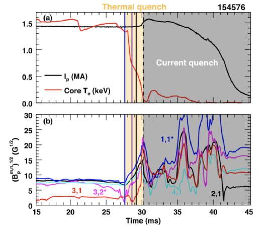
Figure 1: DIII-D shot 154576 [8], where $T_{e}$ in the upper frame is the temperature on a core magnetic surface, and $I_{p}$ is the toroidal current. The lower frame shows magnetic probe signals, dominated by $n=1$ toroidal harmonics. The TQ time is $\tau_{TQ}=.5\tau_{wall}=2.5ms,$ and $\tau_{wall}=5ms$. Reprinted from [8] with IAEA permission.

2 Linear stability

The RWTM dispersion relation generalizes the standard tearing mode by taking into account diffusion of the magnetic perturbation across the resistive wall. This can be expressed for a thin wall as $\gamma\psi=(\eta_{w}/\delta_{w})(\psi^{\prime}_{vac}-\psi^{\prime})$ where $\psi$ is the magnetic potential at the wall, $\psi^{\prime}$ is its radial derivative on the plasma side of the wall, $\gamma$ is the growth rate, $\eta_{w},\delta_{w}$ are the wall resistivity and thickness, and $\psi^{\prime}_{vac}=-(m/r_{w})\psi$ is the radial derivative of $\psi$ on the vacuum side of the wall, where $r_{w}$ is the wall radius and $m$ is the polodal mode number. This can be expressed

$$\left(1+\frac{\gamma\tau_{wall}}{m}\right)\psi=-\frac{r_{w}}{m}\psi^{\prime},$$ (1)

giving a logarithmic derivative boundary condition for $\psi$ at a resistive wall, instead of $\psi=0$ at an ideal wall. The resistive wall penetration time is $\tau_{wall}=r_{w}\delta_{w}/\eta_{w}.$ The RWTM dispersion relation is derived like that of a tearing mode, using the boundary condition (1).

The dispersion relation [1, 11] is

$$\hat{\gamma}^{5/4}{S}^{3/4}=\Delta_{i}+\frac{\Delta_{x}}{\hat{\gamma}{S}_{w}+1}$$ (2)

where $\hat{\gamma}=\gamma\tau_{A},$ $S$ is the Lundquist number, $\tau_{A}=R/v_{A}$ is the Alfvén time, $R$ is the major radius, $v_{A}$ is the Alfvén speed, $S_{w}=S_{wall}(1-x_{s}^{2m})/(2m),$ $S_{wall}=\tau_{wall}/\tau_{A},$ ideal wall stability parameter $\Delta_{i}=r_{s}\Delta_{ideal}^{\prime}/m,$ external stability parameter $\Delta_{x}=2x_{s}^{2m}/(1-x_{s}^{2m})$, $x_{s}=(r_{s}/r_{w}),$ with rational surface radius $r_{s}$.

Ideal wall tearing modes are obtained from (2) in the limit $S_{w}\rightarrow\infty,$ while modes with a highly resistive wall are obtained in the limit $S_{w}\rightarrow 0,$

$$\hat{\gamma}=[(\Delta_{i}+\Delta_{x})]^{4/5}S^{-3/5}.$$ (3)

Resistive wall tearing modes have $\Delta_{i}\leq 0,$ and require finite $S_{w}.$ The RWTM growth rate scalings can be approximated from (2). If $\Delta_{i}=0,$ then assuming $\hat{\gamma}{S}_{w}\gg 1$ [1],

$$\hat{\gamma}=\Delta_{x}^{4/9}S^{-1/3}S_{w}^{-4/9}.$$ (4)

If $\Delta_{i}<0$ and $\Delta_{x}+\Delta_{i}>0$, then neglecting the left side of (2) gives a kind of RWM with rational surface in the plasma,

$$\hat{\gamma}=-\left(1+\frac{\Delta_{x}}{\Delta_{i}}\right)S_{w}^{-1}.$$ (5)

If $\Delta_{i}+\Delta_{x}<0$ there are no unstable solutions of (2). Intermediate asymptotic scalings of $\hat{\gamma}$ are possible depending on the ratio $\Delta_{i}/\Delta_{x},$ as in Fig. 2(a).

The dispersion relation can include a generalized Ohm’s law in the tearing layer, including diamagnetic drifts. These effects are expected to be small, particularly in the limit (5) which does not contain the resistivity. Toroidal rotation is known to stabilize these modes [12, 13, 14]. The required rotation frequency is comparable to the TM linear growth rate. After mode locking, the residual rotation is not enough to stabilize the mode.

We now turn to numerical solutions of the equilibrium reconstruction of DIII-D shot 154576. Linear stability was studied using the M3D-C1 [15] code, with a resistive wall [16]. The reconstruction had on axis safety factor $q_{0}>1$ to prevent the $(1,1)$ mode from dominating the simulations. It represents the equilibrium just before the TQ. The equilibrium is axisymmetric and does not include magnetic islands. Fig. 2(a) shows the growth rate, as a function of $S_{wall}.$ The curve labelled $-1/5$ has $\Delta_{x}=1,$ $\Delta_{i}=-1/5$, which asymptotes to $\gamma\propto S_{wall}^{-2/3}$. The $S_{wall}=0$ limit is a tearing mode with highly resistive wall. The numerical solution is intermediate between the scalings (4) and (5).

Fig. 2(b) shows the perturbed magnetic flux $\psi,$ showing a $(2,1)$ structure. When the wall is ideally conducting, the mode is stable. This shows that the mode is not an ideal wall TM. It must necessarily have $\Delta_{i}\leq 0.$

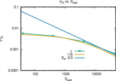
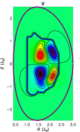
(a) (b)

Figure 2: (a) $\gamma\tau_{A}$ in DIIID shot 154576 as a function of $S_{wall}$ from M3D-C1 linear simulations. The fit is to a RWTM with $\Delta_{x}=1,$ $\Delta_{i}=-1/5,$ from the linear dispersion relation, which asymptotes to $S_{wall}^{-2/3}.$ (b) perturbed $\psi$ in (a). The mode is $(2,1)$, and penetrates the resistive wall.

3 Nonlinear simulations

The linear simulations establish that the equilibrium reconstruction is unstable to a RWTM, and stable to an ideal wall TM. Nonlinear simulations show that the mode grows to large amplitude, sufficient to cause a thermal quench. The simulations were performed with M3D [17] with a thin resistive wall [18]. The simulations used the same parameters as [1, 2], in particular $S=10^{6}$, parallel thermal conductivity $\chi_{\parallel}=10R^{2}/\tau_{A},$ perpendicular thermal conduction and viscosity $\chi_{\perp}=\mu=10^{-4}a^{2}/\tau_{A},$ where $a$ is the minor radius. The simulations used $16$ poloidal planes, adequate to resolve low toroidal mode numbers. The simulations and the experimental data were dominated by $n=1$ modes.

Fig. 3 shows a simulation with M3D [17] with a resistive wall [18], of the same equilibrium reconstruction of DIII-D 154576. The simulation had $S_{wall}=10^{4}.$ Experimentally, $S_{wall}=1.2\times 10^{4}.$ The initial magnetic flux $\psi$ is shown in Fig. 3(a), and the perturbed $\psi$ is in Fig. 3(b), at a time late in the simulation, when the TQ is almost complete. The nonlinear perturbed $\psi$ is predominantly $(2,1)$, similar to the linear structure of Fig. 2(b). The pressure, shown at the same time in Fig. 3(c) has a large perturbation that causes the TQ. The pressure is shown when the total volume integral of the pressure $P$ is about 20% of its initial value.

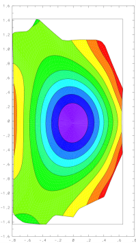
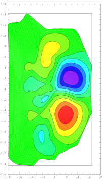
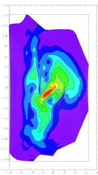
(a) (b) (c)

Figure 3: (a) initial $\psi$ of DIII-D 154576. (b) perturbed $\psi$ at $t=5690\tau_{A},$ $S_{wall}=10^{4}.$ (c) $p$ at $t=5690\tau_{A}.$ when $P$ is about 20% of its initial value.

Fig. 4 shows several M3D simulations with different values of $S_{wall}$. Fig. 4(a) shows time histories of $P$ and $b_{n},$ where $b_{n}$ is the perturbed normal $\delta B/B$ at the wall. The curves are labelled by the value of $S_{wall}.$ All mode numbers $n>0$ are included in $b_{n}.$ Fig. 4(b) shows the TQ time $\tau_{TQ}$ measured from the time histories of $P$. Also shown is $\tau_{\parallel},$ the parallel transport time, given by [1, 2]

$$\tau_{\parallel}=\frac{a^{2}}{\chi_{\parallel}b_{n}^{2}}$$ (6)

using the maximum value of $b_{n}$ for each $S_{wall}$ in Fig. 4(a). The fits are to $3.4/\gamma_{s},$ where the growth rate $\gamma_{s}$ is measured from the time histories of $b_{n}$ in Fig. 4(a), and to $S_{wall}^{2/3}.$ This agrees with Fig. 2(a). The relation $\tau_{\parallel}\propto S_{wall}^{2/3}$ gives the scaling $b_{n}\propto S_{wall}^{-1/3},$ which also agrees with Fig. 5. The vertical line is the experimental value of $S_{wall}.$ At the vertical line $\tau_{TQ}/\tau_{A}\approx 0.4S_{wall},$ or $2ms,$ consistent with experimental data. The mode growth occurs on the same time scale as the TQ, as in the experiment. The small drop in $P$ in Fig. 4(a) at $t\approx 3000\tau_{A}$ is due to internal modes. This resembles the minor precursor disruptions observed in JET [1] and DIII-D [8], which can be seen in Fig. 1.

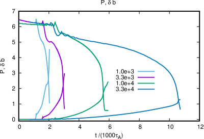
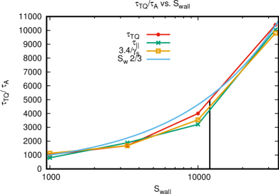
(a) (b)

Figure 4: (a) time histories of $P$ and $b_{n}$ in M3D simulations of DIII-D 154576, where $P$ is total pressure, $b_{n}$ is perturbed normal $\delta B/B$ at the wall. The curves are labeled by the value of $S_{wall}.$ (b) TQ time $\tau_{TQ}$ measured from the time histories of $P$. Also shown is $\tau_{\parallel},$ the parallel transport time (6). The fits are to $3.4/\gamma_{s},$ where $\gamma_{s}$ is measured from the time histories of $b_{n}$ in Fig. 4(a), and to $S_{wall}^{2/3}.$ The vertical line is the experimental value of $S_{wall}.$ At the vertical line $\tau_{TQ}/\tau_{A}\approx 0.4S_{wall},$ consistent with experimental data.

The reason the mode grows to large amplitude may be the external stability parameter $\Delta_{x}.$ TMs have internal stability parameter which depends on the current profile. Growth of an island flattens the current gradient and stabilizes the TM at a moderate amplitude. The external stability parameter $\Delta_{x}$ depends only on $x_{s},$ independent of island size. It is not saturated by local flattening of the current profile. It saturates by driving the $q=2$ surface to the origin, $r_{s}=0.$ This is evident from the $m=2$ structure in $p$ near the axis in Fig. 3(c).

The experimental value of $\delta B/B$ is in agreement with the simulations. At its maximum value, the $(2,1)$ magnetic perturbation in Fig. 1 is $\delta B\approx 480G,$ or $\delta B/B=2.8\times 10^{-2},$ taking $B=1.7T.$ The value of $\delta B$, measured by probes, was estimated [8] at the $(2,1)$ rational surface $r_{s}$, as noted in the discussion of Fig. 1 above. To obtain its value $b_{w}$ at the wall, $\delta B/B$ must be multiplied by $x_{s}^{3}=0.3,$ where $x_{s}=.67,$ yielding $b_{w}=8.4\times 10^{-3}.$ To compare with the simulation, Fig. 5 shows $b_{l}$, the peak transverse perturbed magnetic field at the wall as a function of $S_{wall},$ and peak $b_{n}$, also shown in Fig. 4(a), in units of $10^{-3}.$ The $b_{n}$ signal would be measured by saddle coils in the experiment, while $b_{l}$ would be measured by probes, like $b_{w}.$ The peak value of $b_{l}$ can be fit using (1), with $(b_{n},b_{l})\propto(m\psi/r_{w},\psi^{\prime})$, noting that $\gamma\tau_{wall}b_{n}=const.$ The fit is $b_{n}\approx 0.05S_{wall}^{-1/3},$ $b_{l}=b_{n}+6.7\times 10^{-3}.$ The maximum value $b_{l}=8.8\times 10^{-3}$ at the experimental value $S_{wall}=1.2\times 10^{4}$, is in agreement with $b_{w}.$ The experimental value is indicated in Fig. 5.

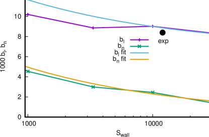
Figure 5: Peak values of $b_{l}$ and $b_{n}$ in units of $10^{-3},$ as a function of $S_{wall}$ in the simulations of Fig. 4(b). The fits are to $b_{n}=0.05S_{wall}^{-1/3},$ $b_{l}=b_{n}+6.7\times 10^{-3}.$ The experimental value is indicated.

4 Onset condition

Having shown that the equilibrium reconstruction is unstable to a RWTM that grows large enough to produce a TQ, we consider the onset condition for the RWTM, $\Delta_{i}=0.$ Both $\Delta_{x}$ and $\Delta_{i}$ depend on $x_{s}.$ In a step current model [11, 19] with a constant current density contained within radius $r_{0}$, with $r_{s}/r_{0}=(2/q_{0})^{1/2},$ and $(m,n)=(2,1)$,

$$\Delta_{i}=-2\frac{q_{0}-1-(q_{0}^{2}/4)x_{s}^{4}}{[q_{0}-1-q_{0}^{2}/4](1-x_{s}^{4})}$$ (7)

For $\Delta_{i}>0$ this requires a positive numerator and negative denominator. If this is not satisfied, the RWTM is unstable,

$$x_{s}^{4}>(4/q_{0}^{2})(q_{0}-1).$$ (8)

For example, if $q_{0}=1.05,$ then $\Delta_{i}=0$ for $x_{s}=0.65.$ For larger $x_{s}>0.65$, the RWTM is unstable. Other current profiles are similar [19], in that larger $x_{s}$ causes $\Delta_{i}\leq 0$. There is additional experimental support for this. Whether a disruption occurs or not depends on the normalized $q=2$ radius $\rho_{q2}$ in a database of DIII-D locked modes [9] Here $\rho_{q2}\approx r_{s}/a,$ and $r_{w}/a\approx 1.2.$ The disruption onset boundary in the database is $\rho_{q2}>0.75,$ or $x_{s}>0.625.$ In the simulations, $\rho_{q2}=0.8,$ so that $x_{s}=0.67.$ The onset condition is that the $q=2$ surface is close enough to the plasma edge. The database also shows that $\rho_{q2}$ increases in time from the beginning to the end of the locked mode, as the disruption is approached. This connects the onset condition to profile evolution.

5 Summary and implications for ITER

To summarize, theory and simulations were presented of resistive wall tearing modes, in an equilibrium reconstruction of DIII-D shot 154576. The linear tearing mode dispersion relation with a resistive wall showed the parameter dependence of the modes, especially on $S_{wall}.$ Linear simulations found that the equilibrium was stable with an ideally conducting wall, and unstable with a resistive wall. For the particular example studied here, the growth rate scales as $\gamma\propto S_{wall}^{-2/3}.$ The RWTMs grow to large amplitude nonlinearly. The thermal quench time is proportional to the RWTM growth time. The amplitude of the simulated peak magnetic perturbations is in agreement with the experimental data. The onset condition for disruptions is that the $q=2$ rational surface is close enough to the plasma edge, consistent with a DIII-D disruption database.

These results are very favorable for ITER disruptions. The ITER resistive wall time, $250ms,$ is $50$ times longer than in JET and DIII-D. The TQ time, instead of being $1.5-2.5ms$ in JET and DIII-D respectively, could be $75-125ms,$ assuming the TQ is produced by a RWTM with $\tau_{TQ}\approx\tau_{wall}/2$ scaling. If the TQ is caused by a RWTM with $S_{wall}^{-4/9}$, and the edge temperature is $500eV,$ then [2] $\tau_{TQ}=70ms.$ The highly conducting ITER wall strongly mitigates RWTMs. It could greatly relax the requirements of the disruption mitigation system, disruption prediction, and mitigation of runaway electrons.

Acknowledgement This work was supported by U.S. DOE under DE-SC0020127, DE-FC02-04ER54698, and by Subcontract S015879 with Princeton Plasma Physics Laboratory. The help of R. Sweeney with the DIII-D data and for discussions is acknowledged.

Data Availability The data that support the findings of this study are available from the corresponding author upon reasonable request.

References

- [1] H. Strauss and JET Contributors, Effect of Resistive Wall on Thermal Quench in JET Disruptions, Phys. Plasmas 28, 032501 (2021)
- [2] H. Strauss, Thermal quench in ITER disruptions, Phys. Plasmas 28 072507 (2021)
- [3] P.C. de Vries, M.F. Johnson, B. Alper, P. Buratti, T.C. Hender, H.R. Koslowski, V. Riccardo and JET-EFDA Contributors, Survey of disruption causes at JET, Nucl. Fusion 51 053018 (2011).
- [4] S.N. Gerasimov, P. Abreu, G. Artaserse, M. Baruzzo, P. Buratti, I.S. Carvalho, I.H. Coffey, E. De La Luna, T.C. Hender, R.B. Henriques, R. Felton, S. Jachmich, U. Kruezi, P.J. Lomas, P. McCullen, M. Maslov, E. Matveeva, S. Moradi, L. Piron1, F.G. Rimini, W. Schippers, C. Stuart, G. Szepesi, M. Tsalas, D. Valcarcel, L.E. Zakharov and JET Contributors, Overview of disruptions with JET-ILW, Nucl. Fusion 60 066028 (2020).
- [5] P.C. de Vries, G. Pautasso, E. Nardon, P. Cahyna, S. Gerasimov, J. Havlicek, T.C. Hender, G.T.A. Huijsmans, M. Lehnen, M. Maraschek, T. Markovič, J.A. Snipes and the COMPASS Team, the ASDEX Upgrade Team and JET Contributors Scaling of the MHD perturbation amplitude required to trigger a disruption and predictions for ITER, Nucl. Fusion 56 026007 (2016).
- [6] F.C. Schuller, Disruptions in tokamaks, Plasma Phys. Controlled Fusion 37, A135 (1995).
- [7] G. Pucella, P. Buratti, E. Giovannozzi, E. Alessi, F. Auriemma, D. Brunetti, D. R. Ferreira, M. Baruzzo, D. Frigione, L. Garzotti, E. Joffrin, E. Lerche, P. J. Lomas, S. Nowak, L. Piron, F. Rimini, C. Sozzi, D. Van Eester, and JET Contributors, Tearing modes in plasma termination on JET: the role of temperature hollowing and edge cooling, Nucl. Fusion 61 046020 (2021)
- [8] R. Sweeney, W. Choi, M. Austin, M. Brookman, V. Izzo, M. Knolker, R.J. La Haye, A. Leonard, E. Strait, F.A. Volpe and The DIII-D Team, Relationship between locked modes and thermal quenches in DIII-D, Nucl. Fusion 58, 056022 (2018)
- [9] R. Sweeney, W. Choi, R. J. La Haye, S. Mao, K. E. J. Olofsson, F. A. Volpe, and the DIII-D Team, Statistical analysis of m/n = 2/1 locked and quasi - stationary modes with rotating precursors in DIII-D, Nucl. Fusion 57 0160192 (2017)
- [10] M.Lehnen, K.Aleynikova, P.B.Aleynikov, D.J.Campbell, P.Drewelow, N.W.Eidietis, Yu.Gasparyan, R.S.Granetz, Y.Gribov, N.Hartmann, E.M.Hollmann, V.A.Izzo, S.Jachmich, S.-H.Kim, M.Kočan, H.R.Koslowski, D.Kovalenko, U.Kruezi, A.Loarte, S.Maruyama, G.F.Matthews, P.B.Parks, G.Pautasso, R.A.Pitts, C.Reux, V.Riccardo, R.Roccella, J.A.Snipes, A.J.Thornton, P.C.de Vries, EFDA JET contributors, Disruptions in ITER and strategies for their control and mitigation, Journal of Nuclear Materials, 463, 39 (2015)
- [11] John A. Finn, Resistive wall stabilization of kink and tearing modes Phys. Plasmas 2, 198 (1995)
- [12] C.G. Gimblett, On free boundary instabilities induced by a resistive wall, Nucl. Fusion 26, 617 (1986)
- [13] A. Bondeson and M. Persson, Stabilization by resistive walls and q-limit disruptions in tokamaks, Nucl. Fusion 28, 1887 (1988)
- [14] R. Betti, Beta limits for the n = 1 mode in rotating - toroidal - resistive plasmas surrounded by a resistive wall, Phys. Plasmas 5, 3615 (1998).
- [15] S. C. Jardin, N. Ferraro, J. Breslau, J. and Chen, Comput. Sci. & Disc., 5, 014002 (2012)
- [16] N.M. Ferraro, S. C. Jardin, L. L. Lao, M. S. Shephard, and F. Zang, Multi - region approach to free - boundary three - dimensional tokakmak equilibria and resistive wall instabilities, Phys. Plasmas 23, 056114 (2016).
- [17] W. Park, E. Belova, G. Y. Fu, X. Tang, H. R. Strauss, L. E. Sugiyama, Plasma Simulation Studies using Multilevel Physics Models, Phys. Plasmas 6 1796 (1999).
- [18] A. Pletzer and H. Strauss, Comput. Phys. Commun. 182, 2077 (2011).
- [19] H. P. Furth, P. H. Rutherford, and H. Selberg, Tearing mode in the cylindrical tokamak, Physics of Fluids 16, 1054 (1973)