Time Optimization of Constrained Control
for a Thermoelectric Solid System
with a Peltier Element

Abstract

A solid system consisting of two heat conducting cylinders with a thermoelectric converter (Peltier element) between them is considered. A nonlinear model, which was previously verified by authors, is used to design a constrained control law that allows us to achieve a steady-state distribution of the temperature in one of the cylinders in much less time than the characteristic time of transient processes. The initial-boundary value problem is exactly linearized over temperature by means of feedback linearization. Although the resulting system is nonlinear in a control function, it is possible to construct a finite-dimensional approximation based on analytical solution of the corresponding eigenproblem for a constant control signal. The time-optimal control problem is studied numerically by using this eigenfunction decomposition. To construct admissible control laws, an auxiliary unconstrained optimization problem is introduced. Its cost functional represents a weighted sum of temperature deviation from the desired zero distribution and a penalty for violating an electric power constraint. The control time interval is split into several parts, and on each subinterval the control signal is taken constant. The optimal piecewise constant feedforward control is found numerically by applying the gradient descent method. We analyze the proposed control law with respect to the shortest admissible time of the process.

Keywords Time-optimal control  $\cdot$ Constrained Optimization  $\cdot$ Thermoelectric Solid System  $\cdot$ Peltier Element.

1 Introduction

At present, solid-state thermoelectric converters, including Peltier elements (PEs), are increasingly used in technical applications. Despite moderate power of such devices, they have a number of significant advantages, such as compactness, resistance to external disturbances, accuracy and fast response rate of control signals. Applying thermoelectric converters as actuators and sensors makes it possible to create efficient heat transfer systems and control various technological processes to achieve and maintain certain temperature regimes in solids. The examples of such application, including systems utilizing renewable energy sources, can be found in farming [1], machining [2], energy generation [3], air conditioning [4], water heating [5] and cooling [6]. For the control of such systems, a wide variety of methods is used from bang-bang type control [7] to classical PI controllers as well as neural network control models [8].

To construct accurate control laws, it is necessary to use coupled nonlinear thermoelectric models that take into account effects of electric energy recuperation, Joule heat losses, and heat exchange with the environment. Given limitations imposed on the power consumption of a PE, it is important to evaluate both reachability ranges for admissible input signals and the minimal time in which the system can be transfered to the desired state. Even for relatively simple systems, a direct solution of the time-optimal control problem seems to be a rather difficult goal. Therefore, one can use different approaches to numerically estimate the minimum of control time. In this paper, we apply the gradient descent method for this purpose. For a system consisting of two metal cylinders and a Peltier disk-like element separating them, we try to reach a small neighborhood of the desired terminal state, while the constraints on the electric current are taken into account utilizing a penalty term added to the cost functional.

2 Model of a Thermoelectric Converter

A full controlled plant may contain many actuated elements consisting of parts with complex geometry and inhomogeneous parameters, what hinders a study of limiting behavior. For this reason, as a simple example we consider a thermoelectric system consisting of two identical heat conducting cylinders and a thin circular PE between them, see Fig. 1. The length of the cylinders and the PE are $z_{1}-z_{0}$ and $2z_{0},$ respectively, where $z_{0}\ll z_{1}.$ Their radii are equal to $r_{1}.$ A corresponding experimental setup was constructed at the Chair of Mechatronics of the University of Rostock, Germany [9], [10].

Figure 1: Schematic representation of the experimental setup.

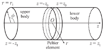
Under assumption that the PE characteristics are constant and heat transfer in the PE occurs only in one direction, a nonlinear model of thermoelectric processes was proposed and validated in [9], [10], [11], [12]. The governing equations of this model were simplified by introducing a feedback linearization control in [14]. The resulting initial-boundary value problem (IBVP) has the following form in cylindrical coordinates $\mathbf{x}=(r,\phi,z)$

$$\begin{array}[]{c}c_{p}\rho_{p}\dot{\theta}=\lambda_{p}\theta^{\prime\prime}_{zz}+\frac{u^{2}}{R|\mathcal{V}_{p}|},\quad\mathbf{x}\in\mathcal{V}_{p},\\ c_{a}\rho_{a}\dot{\theta}=\lambda_{a}\Delta\theta,\quad\mathbf{x}\in\mathcal{V}_{k},\quad k=1,2,\\ \theta^{\prime}_{z}|_{|z|=z_{1}}=0,\quad\alpha\theta+\lambda_{a}\theta^{\prime}_{r}|_{r=r_{1},|z|>z_{0}}=\alpha\theta_{A},\\ \theta|_{|z|=z_{0}\pm 0}=\theta|_{|z|=z_{0}\mp 0},\\ \left.-\lambda_{a}\theta^{\prime}_{z}\right|_{|z|=z_{0}+0}=\left[(\theta+\theta^{0})\frac{Su}{R|\mathcal{A}_{p}|}-\lambda_{p}\theta^{\prime}_{z}\right]_{|z|=z_{0}-0},\\ \theta(0,\mathbf{x})=\Theta(\mathbf{x}),\\ u(t)=\left\{\begin{array}[]{ll}u_{0}(t)-u_{-}&\mathrm{for}\quad u_{0}<u_{-}\\ 0&\mathrm{for}\quad u_{-}\leq u_{0}\leq u_{+}\\ u_{0}(t)-u_{+}&\mathrm{for}\quad u_{0}>u_{+}\\ \end{array}.\right.\end{array}$$ (1)

Here, $c_{p,a}$ are specific heat capacities, $\rho_{p,a}$ are densities, $\lambda_{p,a}$ are thermal conductivities for the PE ($p$) and the cylinders ($a$), $\alpha$ is the heat transfer coefficient, $\theta_{A}$ and $\theta^{0}$ are the constant ambient and reference temperatures, respectively, $|\mathcal{A}_{p}|=\pi r_{1}^{2},$ $S$ is the Seebeck coefficient, and $R$ is the ohmic resistance of the PE. The cylinders and the PE occupy domains $\mathcal{V}_{k}=I_{r}\times I_{\phi}\times I_{k}$ $(k=1,2)$ and $\mathcal{V}_{p}=I_{r}\times I_{\phi}\times I_{p}$, respectively, where $I_{r}=[0,r_{1}],$ $I_{\phi}=[0,2\pi],$ $I_{p}=[-z_{0},z_{0}],$ $I_{1}=[z_{0},z_{1}],$ $I_{2}=[-z_{1},-z_{0}].$ The temperature distribution $\theta(t,\mathbf{x})$ and the ambient temperature are measured relatively to the reference temperature $\theta^{0}$. Although we suppose that $\theta_{A}$ is constant, the proposed approached can be extended to the ambient temperature varying in time [13]. For definiteness, it is assumed that the thermoelectric system (1) is initially in a steady state: $\Theta(\mathbf{x})=\theta_{st},$ such that the cylinder $\mathcal{V}_{1}$ has average temperature $\theta_{av}$, and $u_{st}$ is a constant voltage that yields the temperature distribution $\theta_{st}$.

The control function $u(t)$ is defined through the input voltage $u_{0}(t)$ and thresholds $u_{\pm}$. The total control voltage supplied to the PE is expressed as

$$U=u_{0}+S[\tilde{\theta}].$$ (2)

Here, $[\tilde{\theta}]$ denotes the jump of the average temperature on the top and bottom sides of the PE. Although the voltage $S[\tilde{\theta}]$ provides the linearization w.r.t. the temperature, see [14], the resulting IBVP (1) is still nonlinear in $u$. Therefore, an explicit design of optimal control is hindered. In what follows, we propose a semi-analytical approach to solution of an optimal control problem (OCP) for (1) based on eigenfunction decomposition of $\theta$ for constant values of $u$.

3 Optimal Control Problem

Previously, we considered an OCP for the IBVP (1), where the goal was to achieve a steady-state distribution of the temperature in one of the cylinders. Although both cylinders are actuated by the PE in such a problem, the second cylinder $\mathcal{V}_{2}$ serves only as a “heat sink”, while the first one, $\mathcal{V}_{1}$, represents a controlled part of a plant in which a stable working regime has to be achieved. To this end, we utilized a piecewise control function [14] and took into account disturbances of the ambient temperature [13]. Recently, we optimized a constrained piecewise control signal [15].

Figure 2: Penalty function $f(u)$ vs $u^{2}$.

3.1 Control problem: general statement

In this work, we consider a time-optimal control problem. We suppose that the goal is to return the actuated cylinder to the zero state in a shortest time $T:$

$$T\to\min_{u}\text{ subject to }\frac{\|\theta(T,\mathbf{x})\|_{L_{2}(\mathcal{V}_{1})}}{\|\theta(0,\mathbf{x})\|_{L_{2}(\mathcal{V}_{1})}}\leqslant\varepsilon$$ (3)

as well as the IBVP (1) and constraints on $u$:

$$|u|\leq|u_{st}|.$$ (4)

That is, we suppose that the bounds on $u$ are defined by a control signal $u_{st}$ corresponding to the initial steady state $\theta_{st}.$

3.2 Relaxed control problem

Direct solution of (3), (4) is hindered due to its nonlinearity and uncertainty of existence of global or even local minimum. To deal with these difficulties, we consider a relaxed version of (3), (4) instead of finding exact solution. We find admissible control laws such that $\frac{\|\theta(T,\mathbf{x})\||_{L_{2}(\mathcal{V}_{1})}}{\|\theta(0,\mathbf{x})\||_{L_{2}(\mathcal{V}_{1})}}\leqslant\varepsilon$ and (1), (4) are satisfied. That allows for estimating from above the minimal control time $T_{min}$. To design numerically admissible control laws, we consider an unconstrained optimization problem keeping only (1) as a constraint. To this end, we minimize the cost function

$$\begin{array}[]{c}F\to\min\limits_{u},\quad F=10^{\gamma}F_{d}+F_{p},\quad F_{d}=c_{\theta}\|\theta(T,\mathbf{x})\|^{2}_{L_{2}(\mathcal{V}_{1})},\\[6.45831pt] \displaystyle c_{\theta}=({|\mathcal{V}_{1}|\theta_{av}^{2}})^{-1}{2\pi\int_{0}^{r_{1}}rJ_{0}^{2}(\mu_{0,0}r/r_{1})dr},\end{array}$$ (5)

subject to the IBVP (1). In (5), $J_{0}$ is the Bessel function of zeroth order of the first kind, $\mu_{0,0}$ is a root of an equation presented in the next section. Note that the $L_{2}$-norm in (5) is evaluated only over $\mathcal{V}_{1}.$ That is, we minimize the temperature only in the controlled cylinder $\mathcal{V}_{1}$, while the actuated cylinder $\mathcal{V}_{2}$ may have any temperature yielded by $u$.

The functional $F_{d}$ in (5) represents the norm of the deviation of the temperature distribution from the zero state in the controlled cylinder $\mathcal{V}_{1}$ at time $T$, while

$$F_{p}=c_{u}\int_{0}^{T}f(u)dt,\quad c_{u}=(\rho_{a}c_{a}R|\mathcal{V}_{1}|\theta_{av})^{-1},$$ (6)

is a penalty term.

The penalty functional $F_{p}$ was proposed in [15] and characterized as follows:

$$\begin{array}[]{c}f(u)\sim o(u^{2})\text{ for }|u|<\varepsilon,\quad\varepsilon\ll u_{st},\\ f(u)\ll u^{2}\quad\text{for}\quad|u|<u_{st}-\varepsilon,\\ f(u)\gg u^{2}\quad\text{if}\quad|u|\geq u_{st}.\end{array}$$ (7)

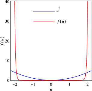
Therefore, $F_{p}$ is small enough if the control function satisfies the constraints and is large otherwise. We define the penalty function according to

$$f(u)=c_{1}(e^{c_{2}u^{2}}-c_{2}u^{2}-1).$$ (8)

The constants $c_{1},c_{2}$ must be chosen such that the conditions (7) are satisfied. See Fig. 2, where these constants are as in the numerical example presented further.

To estimate the minimal control time $T_{min}$ in (3), we solve the problem (5) for an admissible solution via the gradient descend method for $T$ in some range $[T_{0},T_{1}]$ choosing as $T_{min}$ such a value that the constraints (4) are satisfied.

4 Finite Dimensional Approximation

To simplify the studied control problem, we consider a finite dimensional approximation of the IBVP (1). Suppose that $u(t)$ is constant: $u(t)=u^{(i)}$. Then a solution to (1) can be represented as the series

$$\begin{array}[]{c}\theta=\sum_{n,m,k}e^{\nu_{n,m,k}t}\Xi_{n,m,k}(r,\phi,z),\\[6.45831pt] \Xi_{n,m,k}(r,\phi,z)=J_{n}(\mu_{n,m}r/r_{1})\cos(n\phi)\psi_{k}(z),\end{array}$$ (9)

where $\Xi$ are orthogonal eigenfunctions of the IBVP (1). In (9), $J_{n}$ are Bessel functions of the first kind of order $n$, $\mu=\mu_{n,m}$ are roots of the equation

$$\alpha J_{n}(\mu)+\frac{\lambda_{a}}{r_{1}}(nJ_{n}(\mu)-\mu J_{n+1}(\mu))=0,$$ (10)

which corresponds to the boundary condition on the lateral surface of the cylinders. The quantities

$$\nu=\tau^{-1}=-\frac{\lambda_{a}(\mu^{2}+\xi^{2})}{c_{a}\rho_{a}r_{1}^{2}}$$

are the inversed characteristic times of decay $\tau=\tau_{n,m,k}$ of each mode, and $\xi=\xi_{k}$ are eigenvalues corresponding to the eigenfunctions in the $z$-direction $\psi(z)=\psi_{k}(z)$ [14]. These functions are found explicitly as piecewise continuous linear combinations of exponential and trigonometric functions.

Analysis of characteristic times $\tau_{n,m,k}$ allows one to determine the modes that can be neglected on the time interval $[0,T]$ due to their quick decaying. For the experimental setup considered here, only the four lowest modes have characteristic times $\tau_{n,m,k}\gtrsim 10$ sec. For the highest modes, $\tau_{n,m,k}\lesssim 5$ sec, see [14]. Therefore, these transient processes can be excluded from consideration if the intervals of constancy of $u$ are much longer. It is worth mentioning that the angular modes ($n>0$) are uncontrollable in this setting. However, they belong to the group of quickly decaying modes and can be neglected.

Hence, the expansion (9) simplifies to

$$\theta=\sum_{k=0}^{3}e^{\nu_{0,0,k}t}J_{n}(\mu_{0,0}r/r_{1})\psi_{k}(z).$$ (11)

The expansion of the initial steady state $\Theta(\mathbf{x})=\theta_{st}$ w.r.t. to these eigenfunctions yields a vector of coefficients $\bar{\Theta}$. Next, by substituting (11) into (1) and projecting the result onto the eigenfunctions, we obtain the four-dimensional system of ordinary differential equations

$$\begin{array}[]{c}\dot{\bar{\theta}}=A\bar{\theta}+{G}(u,\theta_{A},\theta^{0}),\quad\bar{\theta}(0,z)=\bar{\Theta},\\ \bar{\theta}=(\theta_{0},\ldots,\theta_{3})^{T},\quad\bar{\Theta}=(\Theta_{0},\ldots,\Theta_{3})^{T},\\ \displaystyle\Theta_{i}=\int_{\mathcal{V}}\Theta(\bar{x})\Xi_{i}(\mathbf{x})d\mathbf{x},\quad\Xi_{i}=J_{0}\left(\mu_{0,0}r/{r_{1}}\right)\psi_{0,0,i}.\end{array}$$ (12)

Here, $\theta_{i}=\theta_{0,0,i}$, the matrix $A$ is diagonal consisting of eigenvalues $\nu_{0,0,i}$, and the vector $G$ is constant for a constant $u$. Hence, the system (12) can be solved explicitly for any given initial conditions (ICs) $\bar{\Theta}$.

The steady state $\theta_{st},$ which we take as ICs in (1), is obtained for a given voltage $u_{st}$ in a similar way. Neglecting the rate of temperature change in (1), we plug into the resulting system the ansatz function $\theta_{st}(\mathbf{x})=J_{0}(\mu_{0,0}r/r_{1})\psi_{st}(z)$ and find $\psi_{st}$ as a function of $u_{st}$ explicitly as a piecewise continuous linear combination of cosines and quadratic polynomials.

In its turn, the voltage $u_{st}$ is chosen such that the resulting temperature distribution $\theta_{st}$ has some prescribed average value $\theta_{av}$ in the actuating cylinder: $\theta_{av}=\frac{1}{|\mathcal{V}_{1}|}\int_{\mathcal{V}_{1}}\theta_{st}dV.$ Utilizing the procedure described above and functions $\psi_{st}(u_{st})$, we find $u_{st}$ explicitly by solving the minimization problem

$$\Big{(}\frac{1}{|\mathcal{V}_{1}|}\int\nolimits_{\mathcal{V}_{1}}\theta_{st}dV-\theta_{av}\Big{)}^{2}\to\min\limits_{u}.$$ (13)

5 Solution of the control problem

5.1 Auxiliary optimization problem

Figure 3: The relative value of the cost functional $F$.

In this section, a combined numerical-analytical approach to the solution of OCP (3) is proposed assuming that the control function $u(t)$ is piecewise constant.

For a given $T$, the time interval $[0,T]$ is split into 5 equal subintervals $[t_{i},t_{i+1}]$, $t_{0}=0,$ $t_{5}=T$, $i=0,\ldots,5$. We suppose that $u(t)$ is constant on each subinterval: $u(t)=u^{(i)}\in\mathbb{R}$ for $t\in[t_{i},t_{i+1}].$ For a given $u^{(i)}$, the eigenfunctions $\psi_{k}^{(i)}(z)$ are found according to Sect. 4. Next, we solve explicitly (12) on $[0,t_{1}]$ for the given initial steady state $\bar{\Theta}$ and the control function $u(t)=u^{(0)}.$ The resulting distribution $\theta(t_{1},\mathbf{x})$, which is a linear combination of eigenfunctions $\psi_{k}^{(0)}(z)$, is re-expanded w.r.t. the eigenfunctions $\psi_{k}^{(1)}(z)$ corresponding to $u^{(1)}$. Taking coefficients of this expansion as ICs $\bar{\Theta}^{(1)}$, we solve on $[t_{1},t_{2}]$ the system (12) with a new matrix $A^{(1)}$ determined by eigenvalues $\nu_{k}^{(1)}$. This yields the temperature $\theta(t_{2},\mathbf{x})$. We repeat consequently solution of (12) and re-expansion of $\theta$ until the terminal state $\theta(T,\mathbf{x})$ is reached.

For the fixed time horizon $T$, we find piecewise constant $u=(u^{(0)},\ldots,u^{(4)})^{T}$ such that

$$F[u,\theta]\to\min_{u(t),t\in[0,T]},$$ (14)

where $F$ is defined in (5). This problem is solved via the gradient descend. When starting with a vector

$$\bar{u}^{(0)}=(u^{(0,0)},\ldots,u^{(0,4)}),$$ (15)

the next value is computed according to

$$\bar{u}^{(j+1)}=\bar{u}^{(j)}+\varepsilon\nabla_{\bar{u}}F,\quad\varepsilon\ll 1.$$ (16)

The gradient $\nabla_{\bar{u}}F$ is found numerically via finite differences

$$\frac{F(u^{(j,l)}+\delta u^{(j,l)})-F(u^{(j,l)})}{\delta},\quad\delta\ll 1,$$ (17)

but the values of $F(u^{(j,l)})$ and their variation $F(u^{(j,l)}+\delta u^{(j,l)})$ are obtained analytically by using the algorithm presented in Sect. 4.

5.2 Estimating the minimal time

Figure 4: The norm of the terminal temperature distribution in the controlled cylinder related to the norm of temperature at $t=T$ due to natural cooling.

To estimate the minimal time $T_{min}$, we start with $T_{0}\sim\tau_{0,0,0}$, where $\tau_{0,0,0}$ is the characteristic time of decay of the zeroth eigenmode. For such large $T$, the system loses most of the heat due to natural cooling/heating and the active control is almost not needed. Next, we decrease $T$, $T_{j}=T_{j-1}-\delta T_{0}$ and solve the OCP (14) on the time interval $[0,T_{j}].$ The minimal value of $T_{j}$ such that the solution $u(t)$ of (14) does not violate the constraints, we take as an estimate from above of $T_{min}$.

In the next section, we present a numerical example of implementation of approaches described in Sects. 4, 5.

Figure 5: The norm of the terminal temperature distribution in the controlled cylinder related to the norm of initial temperature distribution.

6 Numerical results and discussion

The following physical parameters corresponding to the experimental setup, see [10], [9], are considered: $\lambda_{a}=254.4$ W/m/K, $\lambda_{p}=0.517$ W/m/K, $\rho_{a}=2700$ kg/m${}^{3},$ $\rho_{p}=3000$ kg/m${}^{3},$ $c_{a}=896$ J/kg/K, $c_{p}=500$ J/kg/K, $\alpha=8.4$ W/m²/K, $h=0.1$ m, $r_{1}=0.031$ m, $z_{0}=0.00195$ m, $z_{1}=z_{0}+h$, $S=0.0427$ W/K/A, $R=6.03$ $\Omega,$ $u_{+}=1.115$ V and $u_{-}=-1.29$ V. We take the reference temperature $\theta^{0}=293$ K, and the initial steady state $\theta_{st}$ such that the average temperature $\theta_{av}$ in the controlled cylinder $\mathcal{V}_{1}$ is $5.5$ K. The voltage $u_{st}$ corresponding to this state is found solving (13): $u_{st}\approx 1.44$ V. We take this value as the constraints: $|u(t)|\leq 1.44$ V. The terminal time $T$ is varied with the step $\delta T_{0}=12$ sec.

Figure 6: The maximum absolute value of the control function $u(t)$: $\max_{t\in[0,T]}|u(t)|$.

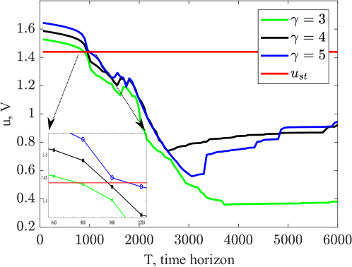
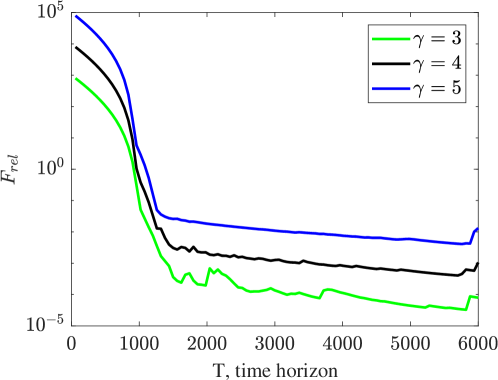
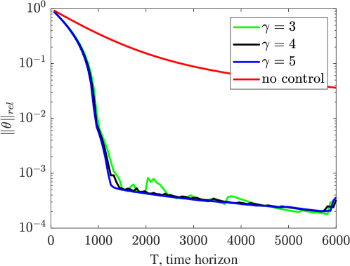
To design admissible control laws, we consider several values of the weighting coefficient $\gamma$ in (5). The larger value of $\gamma$ favors minimization of the temperature rather than satisfaction of the control constraints. In Figs. 3–9 the numerical results for the values of the weighting coefficient $\gamma=3,4,5$ are presented. In Fig. 3, the optimal values of the cost function $F$ (in logarithmic scale) are shown as a function of the time horizon $T$. These values do not change significantly while $T\gg 10^{3}$ sec. In this region, the obtained control laws satisfy constraints and transfer the system to a small neighbourhood of the zero state.

Figure 7: The piecewise control function $u(t)$; $T=1020$ sec.

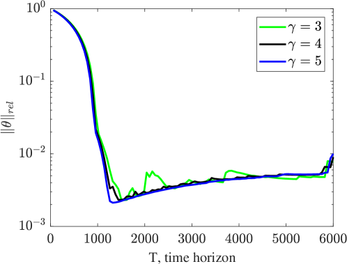
This statement is supported by Figs. 4, 5, where the relative $L_{2}$-norm of the terminal temperature distribution in $\mathcal{V}_{1}$ is given in logarithmic scale. In Fig. 4, these values are normalized by the norm of the temperature in $\mathcal{V}_{1}$ that emerges in this cylinder due to natural cooling during the same time $T$. Therefore, Fig. 4 shows the effectiveness of the control law. As it can be expected, this effectiveness grows as $T$ decreases: on long time intervals the natural cooling is enough to achieve a state close to zero. However, as $T$ becomes smaller, the advantage of an active control is more clear: it allows to make temperature up to 3 order smaller than the natural cooling. Nevertheless, since power required to achieve the zero state grows with decreasing $T$, for $T\gtrsim 10^{3}$ the control law within the constraints loses its advantages and the effectiveness diminishes quickly. Fig. 4 demonstrates the temperature decreasing comparing with the initial steady state. Here, the $L_{2}$-norm of the terminal temperature distribution in $\mathcal{V}_{1}$ (in logarithmic scale) is related to the $L_{2}$-norm of the steady state. The red curve represents the natural cooling.

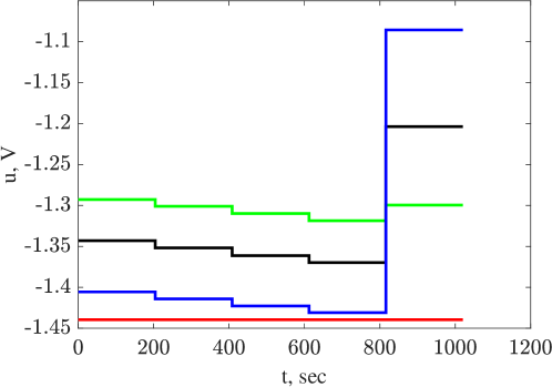
Figs. 6, 7 illustrate the behavior of the optimal control law. Fig. 6 shows the maximum absolute value of $u(t)$. This allows us to estimate $T_{min}$. Fix $\varepsilon=10^{-2}.$ Note that relaxing the temperature minimization (making $\gamma$ smaller) let us achieve smaller values of $T_{min}$: $T_{min}$ for $\gamma=3$ is less then $10^{3}$ sec, but $T_{min}>10^{3}$ sec for $\gamma=4,5.$ In Fig. 7, the piecewise optimal control laws for $\tilde{T}=1020$ sec are given. The control constraint is depicted by the red line. As can be seen for the chosen time step $\delta T_{0}$, this value $\tilde{T}$ may be taken as $T_{min}$ for $\gamma=5.$

Figure 8: The terminal temperature distribution.

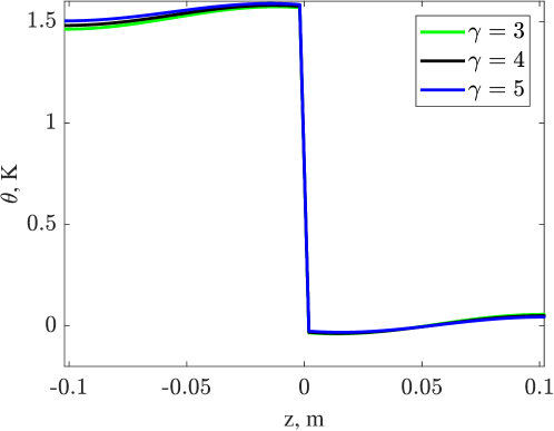
Figs. 8, 9 show the terminal temperature distribution for the weighting coefficients $\gamma=3,4,5$. Here, $T=1020$ sec. Although the control laws are rather different, see Fig. 7, these distributions in the controlled cylinder $\mathcal{V}_{1}$ are close to each other. Note that the distinction between the results of the considered control laws is more pronounced in the uncontrolled cylinder $\mathcal{V}_{2}$ (negative values of $z$), which is used as a heat sink. In Fig.  9, we may compare the initial steady state (dashed line) with the distributions obtained due to natural cooling (red curve) and due to the optimal control law (black curve) for $\gamma=4$. Note the overheating of the uncontrolled cylinder $\mathcal{V}_{2}$. The time $T$ is too short to get to the zero state in $\mathcal{V}_{1}$ via natural cooling and the actuator transfers the energy from $\mathcal{V}_{1}$ to $\mathcal{V}_{2}$ by heating it.

Figure 9: The initial and terminal temperature distribution for the controlled and uncontrolled processes.

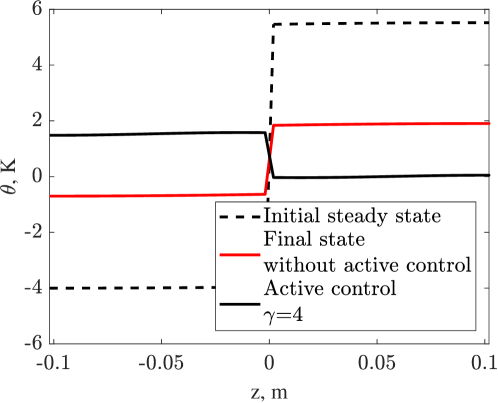
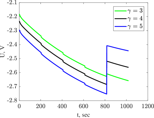
Fig. 10 demonstrates the nonlinear essence of the studied thermoelectric system. The total input voltage involves both feedforward control law $u(t)$ and the feedback linearization signal $S[\tilde{\theta}]$ according to (2). Although $u(t)$ is piecewuse constant, the full input voltage $U(t)$ is more sophisticated, cf. Fig. 7. As the electric current in the PE $Ru$ is proportional to the voltage $u$, the term $S[\tilde{\theta}]$ does not influence on the Joule heat loss.

7 Conclusions

In this paper, we study the constrained time-optimal problem of achieving a prescribed temperature distribution in a thermoelectric solid system. We consider a system consisting of two identical cylinders with a thin Peltier element between them. Although the entire system is actuated by the thermoelectric converter, we try to reach the desired state only in one of them, treating the other cylinder as a heat sink. Assuming that the optimal control law is sought in the class of piecewise constant functions, we reduce the nonlinear PDE system to its finite-dimensional approximation by utilizing eigenfunction decomposition. The constraints are implemented via a penalty term in the cost functional. Next, we vary the time horizon finding an optimal control law with applying the gradient descend method at each step of the variation. On each iteration of the gradient descend, the direct problem is solved explicitly. It has been shown that this combined numerical-analytical approach allows us to reach a rather small neighborhood of the prescribed state without violation of the constraints and estimate from above the minimal control time. We plan to verify proposed strategy and the finite-dimensional approximation exploited by implementing the designed control laws in a FEM setting. Next, we aim at controlling a structure consisting of several heat conducting bodies with Peltier elements between them.

Figure 10: Total input signal with feedback.

References

- [1] Tikhomirov, D.A., Trunov, S.S., Kuzmichev, A.V., Rastimeshin, S., and Shepovalova, O.: Energy-efficient thermoelectric unit for microclimate control on cattlebreeding premises. Energy Rep. 6, 293–305 (2020). doi:10.1016/j.egyr.2020.08.052
- [2] Mironova, A., Haus, B., Zedler, A., and Mercorelli, P.: Extended Kalman filter for temperature estimation and control of Peltier cells in a novel industrial milling process. IEEE Trans. Ind. Appl. 56(2), 1670–1678 (2020). doi:10.1109/TIA.2020.2965058
- [3] Fan, X., Sun, H., Yuan, Z., Li, Z., Shi, R., and Razmjooy, N.: Multi-objective optimization for the proper selection of the best heat pump technology in a fuel cell-heat pump micro-CHP system. Energy Rep., 6, 325–335 (2020). doi:10.1016/j.egyr.2020.01.009
- [4] Moria, H., Pourhedayat, S., Dizaji, H.S., Abusorrah, A.M., Abu-Hamdeh, N.H., and Wae-hayee, M.: Exergoeconomic analysis of a Peltier effect air cooler using experimental data. Appl. Therm. Eng. 186, 116513 (2021). doi:10.1016/j.applthermaleng.2020.116513
- [5] Kwan, T.H., Ikeuchi, D., and Yao, Q.: Application of the Peltier sub-cooled trans-critical carbon dioxide heat pump system for water heating – Modelling and performance analysis. Energy Convers. Manag. 185, 574–585 (2019). doi:10.1016/j.enconman.2019.01.104
- [6] Tijani, I.B., Al Hamadi, A.A., Al Naqbi, K.A., Almarzooqi, R.I., and Al Rahbi, N.K.: Development of an automatic solar-powered domestic water cooling system with multi-stage Peltier devices. Renew. Energy. 128, 416–431 (2018). doi:10.1016/j.renene.2018.05.042
- [7] Badescu, V.: Self-driven reverse thermal engines under monotonous and oscillatory optimal operation. J. Non-Equilib. Thermodyn. 46(3), 291–319 (2021). doi:10.1515/jnet-2020-0103
- [8] Honc, D., Doležel, P., and Merta, J.: Thermal process control using neural model and genetic algorithm. In: R. Silhavy, P. Silhavy, and Z. Prokopova (eds.) Intelligent Systems Applications in Software Engineering. CoMeSySo 2019. Advances in Intelligent Systems and Computing, vol 1046. Springer, Cham (2019). https://doi.org/10.1007/978-3-030-30329-7_35
- [9] Gavrikov, A., Kostin, G., Knyazkov, D., Rauh, A., and Aschemann, H.: Experimental validation of a nonlinear model for controlled thermoelectric processes in cylindrical bodies. In: 24th International Conference on Methods and Models in Automation and Robotics (MMAR), pp. 558–563. IEEE (2019). doi:10.1109/MMAR.2019.8864613
- [10] Knyazkov, D., Kostin, G., Gavrikov, A., Aschemann, H., and Rauh, A.: FEM modeling and parameter identification of thermoelectrical processes in cylindrical bodies. In: 24th International Conference on Methods and Models in Automation and Robotics (MMAR), pp. 501–506. IEEE (2019). doi:10.1109/MMAR.2019.8864704
- [11] Kostin, G.V., Rauh, A., Gavrikov, A., Knyazkov, D., and Aschemann, H.: Heat transfer in cylindrical bodies controlled by a thermoelectric converter. IFAC-PapersOnLine. 52(15), 139–144 (2019). doi:10.1016/j.ifacol.2019.11.664
- [12] Gavrikov, A. and Kostin, G.: A nonlinear model of heat transfer for cylindrical bodies controlled by a thermoelectric converter. In: 15th International Conference on Stability and Oscillations of Nonlinear Control Systems (Pyatnitskiy’s Conference) (STAB), pp. 1–4. IEEE (2020). doi:10.1109/STAB49150.2020.9140683
- [13] Gavrikov, A., Kostin, G., Aschemann, H., and Rauh, A.: Modeling and control of a thermoelectric structure with a Peltier element subject to external disturbances. IFAC-PapersOnLine. 53(2), 7771–7776 (2020). doi:10.1016/j.ifacol.2020.12.1542
- [14] Gavrikov, A., Kostin, G., Knyazkov, D., Rauh, A., and Aschemann, H.: Parameter optimization of control with feedback linearization for a model of thermoelectric processes in cylindrical bodies. In: 24th International Conference on Methods and Models in Automation and Robotics (MMAR), pp. 342–347. IEEE (2019). doi:10.1109/MMAR.2019.8864725
- [15] Gavrikov, A. and Kostin, G.: Feedforward optimal control with constraints for a cylindrical thermoelectric system actuated by a Peltier element. In: XLIX International Summer School-Conference “Advanced Problems in Mechanics” (APM), pp. 1–13. Springer (in print).