Automatic compile-time synthesis of entropy-optimal Boltzmann samplers

Abstract.

We present a framework for the automatic compilation of multi-parametric Boltzmann samplers for algebraic data types in Haskell. Our framework uses Template Haskell to synthesise efficient, entropy-optimal samplers generating random instances of user-declared algebraic data types. Users can control the outcome distribution through a pure, declarative interface. For instance, users can control the mean size and constructor frequencies of generated objects. We illustrate the effectiveness of our framework through a prototype generic-boltzmann-brain library showing that it is possible to control thousands of different parameters in systems of tens of thousands of ADTs. Our prototype framework synthesises Boltzmann samplers capable of rapidly generating random objects of sizes in the millions.

1. Introduction

Consider the following example of a pair of algebraic data types

Lambda} and
\mintinline[fontsize=\small]

haskellDeBruijn defining lambda terms in DeBruijn notation (deBruijn1972):

⬇

data DeBruijn

= Z

| S DeBruijn

\pardata Lambda

= Index DeBruijn

| App Lambda Lambda

| Abs Lambda

In the following paper we develop a general framework for compile-time generation of efficient Boltzmann samplers (DuFlLoSc) for system of algebraic data types, such as 

Lambda} and
\mintinline[fontsize=\small]

haskellDeBruijn. Our prototype library exposes a minimal, declarative Template Haskell (template-haskell) interface. For instance

⬇

mkDefBoltzmannSampler ”Lambda 10_000

declares

Lambda} an instance of the
\mintinline

haskellBoltzmannSampler type class:

⬇

class BoltzmannSampler a where

sample :: RandomGen g =>

UpperBound ->

MaybeT (BuffonMachine g) (a, Int)

The above type class defines types with a single

sample} function.  Given an integer upper
bound $n$, \mintinline[fontsize=\small]

haskellsample generates a random instance $\gamma$ of type

a} together with its
corresponding size $s \leq n$. While computing a random
\mintinline[fontsize=\small]

haskella, the generator consumes random bits provided within a custom

BuffonMachine g}
monad. Because the generation process might sometimes fail, the whole
computation is wrapped in a \mintinline[fontsize=\small]

haskellMaybeT monad transformer. The

sample} function satisfies two key
Boltzmann sampler properties:
\begin

itemize instances of a} with the \emphexact same size have the exact same probability of being generated, and the expected size of the generated instances of

a} follows the user-declared value,
        such as $10,000$ for \mintinline[fontsize=\small]

haskellLambda. In other words, while the size of the outcomes may vary, the outcome distribution is fair, i.e. uniform when conditioned on the size of the generated objects. When a finer control over the outcome size is required, rejection sampling can be adopted cf. (BodLumRolin):

⬇

rejectionSampler ::

(RandomGen g, BoltzmannSampler a) =>

LowerBound -> UpperBound -> BuffonMachine g a

Given two lower and upper bounds, a rejection sampler generates random instances of

a} until a sample of admissible size is
generated. The expected runtime complexity of such a sampler depends on the
\emph

width of the admissible size window. If it is an interval of the form $[(1-\varepsilon)n,(1+\varepsilon)n]$ for some positive tolerance parameter $\varepsilon>0$, the runtime complexity of the rejection sampler is linear, i.e. $O(n)$. When the tolerance parameter $\varepsilon$ is equal to $0$, the rejection sampler returns objects of some constant size $n$, and the expected runtime of

rejectionSampler}
becomes $O(n^

2)$,~{}\emph{cf.}~{}\cite[citep]{(\@@bibref{AuthorsPhrase1Year}{BodLumRolin,DuFlLoSc}{\@@citephrase{, }}{})}.\par Compiledrejectionsamplersarereadilyavailableforuseinpropertytestingframeworks,suchasQuickCheck~{}\cite[citep]{(\@@bibref{AuthorsPhrase1Year}{Claessen-2000}{\@@citephrase{, }}{})}.Forinstance,\verb{BuffonMachine g} computations can be easily converted to QuickCheck's \mintinline[fontsize=\small]{haskell$Gen values:

⬇

quickCheckRejectionSampler ::

BoltzmannSampler a =>

(Int -> (LowerBound, UpperBound)) -> Gen a

By default, the size of generated objects is equal to the overall weight of constructors used in their construction. For instance, the size of

Abs (App (Index Z) (Index Z))} is equal
to six as it consists of size constructor of default weight one. If such a
\emph

size notion is not desired, it is possible to redefine the constructor weights, e.g. as follows:

⬇

mkBoltzmannSampler

System

{ targetType = ”Lambda

, meanSize = 10_000

, frequencies = def

, weights =

(’Index, 0)

<:> $(mkDefWeights ”Lambda)

}

Note that here we declared a Boltzmann sampler for

Lambda}
with (expected) mean size $10,000$, and a new set of \emph

constructor weights in which all constructors except

Index} have default weight one.
The remaining \mintinline[fontsize=\small]

haskellIndex constructor contributes now weight zero to the overall size of lambda terms.

1.1. Beyond uniform outcome distribution

In (BodPonty) a generalisation of Boltzmann samplers was introduced which lifted the classic univariate Boltzmann samplers to a multi-parametric setting. This multivariate paradigm is reflected in the presented framework in form of custom constructor frequencies. For instance

⬇

mkBoltzmannSampler

System

{ targetType = ”Lambda

, meanSize = 10_000

, frequencies = (’Abs, 4_000) <:> def

, weights =

(’Index, 0)

<:> $(mkDefWeights ”Lambda)

}

declares a multi-parametric Boltzmann sampler for

Lambda}
in which the target mean size is still $10,000$, however now we additionally require
that the \emph

mean weight contribution of abstractions is equal to $4,000$. The

size} function satisfies now
the following generalised Boltzmann sampler properties:
\begin

itemize instances of

Lambda} with the exact
        same size \emph

and the same cummulative abstraction weights have the exact same probability of being generated, and the expected size of the generated instances is still $10,000$, whereas the expected number of abstractions is equal to the user-declared value of $4,000$. It is therefore possible to tune the natural frequency of each constructor in

Lambda} and
\mintinline[fontsize=\small]

haskellDeBruijn to one’s needs. Note however that such an additional control causes a significant change in the underlying outcome distribution. In extreme cases, such as for instance requiring 80% of internal nodes in plane binary trees, the sampler might fail to compile or be virtually ineffective due to the sparsity of tuned structures.

1.2. Multiple Boltzmann sampler instances

Because Boltzmann samplers are implemented as instances of the

BoltzmannSampler} type class, we cannot
have two distinct Boltzmann samplers for the same type \mintinline[fontsize=\small]

haskella. In some circumstances, however, having multiple Boltzmann samplers with different constructor frequencies or even size notions might be beneficial. To enable such use cases, the presented framework lets users define Boltzmann samplers for

newtype}s
of respective types.
For instance, in the following snippet we define a representation of so-called
\emph

binary lambda terms, initially introduced by Tromp (tromp) for the purpose of using lambda calculus in algorithmic information theory (cf. also (grygiel_lescanne_2015)):

⬇

newtype BinLambda = MkBinLambda Lambda

\parmkBoltzmannSampler

System

{ targetType = ”BinLambda

, meanSize = 12_000

, frequencies = (’Abs, 3000) <:> def

, weights =

(’Index, 0)

<:> (’App, 2)

<:> (’Abs, 2)

<:> $(mkDefWeights ”Lambda)

}

The

BinLambda} type borrows the algebraic representation
of \mintinline[fontsize=\small]

haskellLambda. Custom weights for

App}
and \mintinline[fontsize=\small]

haskellAbs reflect Tromp’s recursive binary string representation of lambda terms:

⬇

encode :: Lambda -> [Bool]

encode = \caseAbs t -> False : False : encode t

App lt rt -> False : True : encode lt ++ encode rt

Index n -> encode’ n

where

encode’ :: DeBruijn -> [Bool]

encode’ = \caseS n’ -> True : encode’ n’

Z -> [True]

Note that the size of a binary lambda term corresponds to the length of the corresponding encoded binary string. In addition to a new size notion,

BinLambda}
uses a different set of constructor frequencies, and mean size.
\section

Univariate Boltzmann models Before explaining the general architecture of our framework let us pause for a moment and focus on the mathematical foundations of Boltzmann samplers, cf. (DuFlLoSc). Let $\mathcal{S}$ be a set of objects endowed with an intrinsic size function $|\cdot|\colon\mathcal{S}\to\mathbb{N}$ with the property that that for all $n\in\mathbb{N}$, the set of objects of $n$ in $\mathcal{S}$ is finite. For such a class of objects, the corresponding (univariate) generating function $S(z)$ is the power series $S(z)$ defined as

(1) $$S(z)=\sum_{n\geq 0}s_{n}z^{n}$$

whose coefficients $\left(s_{n}\right)_{n\geq 0}$ denote the number of objects of size $n$ in $\mathcal{S}$, cf. (wilf). Given a real control parameter $x\in[0,1]$, a Boltzmann model (DuFlLoSc) is a probability distribution in which the probability $\mathbb{P}_{x}(\omega)$ of generating an object $\omega\in\mathcal{S}$ satisfies

(2) $$\mathbb{P}_{x}(\omega)=\frac{x^{|\omega|}}{S(x)}.$$

provided that $S(x)$ is finite. Note that under such a model

• objects of equal size have equal probabilities, and

• the outcome size is varying random variable.

Indeed, note that the probability $\mathbb{P}_{x}(N=n)$ that the size $N$ of a randomly generated object is equal to $n$ satisfies

(3) $$\mathbb{P}_{x}(N=n)=\frac{s_{n}x^{n}}{S(x)}$$

In other words, the outcome size distribution depends both on the control parameter $x$, as well as on the intrinsic size distribution in $\mathcal{S}$, see e.g. subsection 1.2. In consequence, the control parameter $x$ influences the expected (mean) outcome size $\mathbb{E}_{x}(N)$, as well as the standard deviation $\sigma_{x}(N)$:

(4) $$\mathbb{E}_{x}(N)=x\frac{\frac{d}{dx}S(x)}{S(x)}\quad\sigma_{x}(N)=\sqrt{x\frac{d}{dx}\mathbb{E}_{x}(N)}$$

Given access to the values of $S$ and its derivative $\frac{d}{dx}S$ it is possible to use formula (4) and aptly choose a value of the control parameter $x$ so to obtain a Boltzmann model with expect size of outcomes equal to a target mean size $n$. Even though, in general, explicit formulas or numerical oracles for $S(x)$ and $\frac{d}{dx}S(x)$ might not be readily available, we will soon see that for specifications corresponding to algebraic data types, we can construct efficient oracles and thus automatically find apt values for the control parameter.

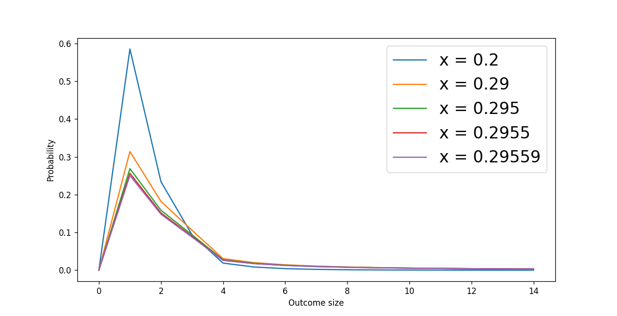
Figure 1. Example univariate Boltzmann models for . Note that the values $\mathbb{P}_{x}(N=n)$ quickly approach zero yet never reach it.

1.3. Compiling Boltzmann samplers

Boltzmann samplers, realising the outcome Boltzmann model, follow closely the sum-of-products structure of ADTs and hence can be compiled in a recursive fashion.

1.3.1. Singletons

Consider a singleton class $\mathcal{S}$, i.e. a set consisting of a single element $\gamma$. Note that the corresponding generating function takes the form $S(z)=z^{|\gamma|}$. Consequently, the probability $\mathbb{P}_{x}(\gamma)$ of sampling $\gamma$ is equal to one, and the respective Boltzmann sampler always returns $\gamma$.

1.3.2. Products

Consider a product class $\mathcal{S}$ consisting of pairs $\gamma=(\alpha,\beta)$ where the components are arbitrary elements of classes $\mathcal{A}$ and $\mathcal{B}$, and $|\gamma|=|\alpha|+|\beta|$. Under a Boltzmann model the probability $\mathbb{P}_{x}(\gamma)$ that $\gamma$ is sampled satisfies

(5) $$\mathbb{P}_{x}(\gamma)=\frac{x^{|\gamma|}}{S(x)}$$

Since $|\gamma|=|\alpha|+|\beta|$ we can rewrite rewrite (5) as

(6) $$\mathbb{P}_{x}(\gamma)=\frac{x^{|\gamma|}}{S(x)}=\frac{x^{|\alpha|+|\beta|}}{S(x)}=\frac{x^{|\alpha|}x^{|\beta|}}{S(x)}$$

Now, let us notice that $S(z)=A(z)B(z)$ as

(7) $$\begin{split}\left(\sum_{n\geq 0}a_{n}z^{n}\right)\cdot\left(\sum_{n\geq 0}b_{n}z^{n}\right)&=\sum_{n\geq 0}c_{n}z^{n}\\ \text{where}\quad c_{n}&=\sum_{k=0}^{n}a_{k}b_{n-k}\end{split}$$

following Cauchy’s product formula for power series. Indeed, the number of pairs $\mathcal{A}\times\mathcal{B}$ of size $n$ is equal to $\sum_{k=0}^{n}a_{k}b_{n-k}$ where $\{a,b\}_{i}$ denotes the number of objects in $\mathcal{A}$ (respectively $\mathcal{B}$) of size $i$. Therefore

(8) $$\mathbb{P}_{x}(\gamma)=\frac{x^{|\alpha|}x^{|\beta|}}{S(x)}=\frac{x^{|\alpha|}x^{|\beta|}}{A(x)B(x)}=\mathbb{P}_{x}(\alpha)\mathbb{P}_{x}(\beta)$$

It means that in order to generate a random pair $\gamma$ corresponding to $\mathcal{S}$ using a Boltzmann sampler, we can invoke Boltzmann samplers for $\mathcal{A}$ and $\mathcal{B}$ using the same control parameter $x$, and then return a pair of their results. Note that the same principle naturally generalises onto for tuples of arbitrary length as $(a,b,c)\cong((a,b),c)\cong(a,(b,c))$.

1.3.3. Coproducts

Consider a coproduct class $\mathcal{S}=\mathcal{A}+\mathcal{B}$ which is a disjoint sum of two classes $\mathcal{A}$ and $\mathcal{B}$. In other words, $\mathcal{S}$ consists of elements $\gamma$ which belong to either $\mathcal{A}$ or $\mathcal{B}$, but not both at the same time. Note that in such a case the probability $\mathbb{P}_{x}(\gamma\in\mathcal{A})$ that an arbitrary object $\gamma$ in $\mathcal{A}$ is sampled satisfies

(9) $$\mathbb{P}_{x}(\gamma\in\mathcal{A})=\frac{A(x)}{S(x)}\quad\text{as}\quad A(x)=\sum_{\gamma\in\mathcal{A}}x^{|\gamma|}$$

It means that in order to generate a random object $\gamma$ in $\mathcal{S}$ using a Boltzmann sampler, we have to make a skewed coin toss. With probability $\frac{A(x)}{S(x)}$ we invoke the sampler corresponding to $\mathcal{A}$, and with probability $\frac{B(x)}{S(x)}$ we invoke the sampler corresponding to $\mathcal{B}$. Like in the case of products, the same principle naturally generalises onto arbitrary sums as $a+b+c\cong(a+b)+c\cong a+(b+c)$.

1.3.4. Algebraic data types

The above simple Boltzmann sampler compilation rules can be readily applied to concrete algebraic data types. Consider our running example system of two ADTs

Lambda} and
\mintinline[fontsize=\small]

haskellDeBruijn. A Boltzmann sampler for

Lambda} has to first make
a random decision which constructor to use,~\emph

i.e.

Abs},
\mintinline[fontsize=\small]

haskellApp, or

Index}.
This decision follows the co-product compilation rule.
If \mintinline[fontsize=\small]

haskellAbs is chosen, following the product rule, the

Lambda}
Boltzmann sampler has to invoke a Boltzmann sampler for \mintinline[fontsize=\small]

haskellLambda (i.e. itself), generate a random lambda term

lt},
and output \mintinline[fontsize=\small]

haskellAbs lt. Likewise, if

App}
is chosen, the \mintinline[fontsize=\small]

haskellLambda Boltzmann sampler has to invoke itself twice, generating two random lambda terms

lt}
and \mintinline[fontsize=\small]

haskelllt’, and output

App lt lt’}.
Finally, if \mintinline[fontsize=\small]

haskellIndex is chosen, the

Lambda}
Boltzmann sampler has to invoke the Boltzmann sampler for \mintinline[fontsize=\small]

haskellDeBruijn which will return a random DeBruijn} index, and wrap it around \mintinline[fontsize=\small]haskellIndex. The Boltzmann sampler for

DeBruijn} is constructed similarly.
Let us remark that while Boltzmann samplers readily apply to algebraic data types, they are not limited to
them. Over the years Boltzmann samplers have enjoyed a series
of extensions and improvements including, \emph

inter alia, the support for so-called labelled (DuFlLoSc), Pólya (flajolet2007boltzmann), or first-order differential specifications (BODINI20122563).

2. Multivariate Boltzmann models

The classical, univariate Boltzmann model controls a single system parameter, i.e. the expected outcome size. In some circumstances, however, a finer control over the outcome distribution is required. Multivariate Boltzmann models, initially introduced in (BodPonty), address this issue by generalising classical Boltzmann models to a multivariate setting in which multiple outcome parameters can be controlled simultaneously. Analogously to their univariate counterparts, multiparametric Boltzmann models depend on multivariate generating functions. A multivariate generating function $S(z_{1},\ldots,z_{d})$ is a power series $S(z_{1},\ldots,z_{d})$ defined as

(10) $$S(z_{1},\ldots,z_{d})=\sum_{n_{1},\ldots,n_{d}\geq 0}s_{n_{1},\ldots,n_{d}}\prod_{i=1}^{d}z_{i}^{n_{i}}$$

whose coefficients $\left(s_{n_{1},\ldots,n_{d}}\right)_{n\geq 0}$ denote the number of objects with $n_{i}$ atoms of type $z_{i}$ in $\mathcal{S}$, cf. (flajolet09). For instance, $z_{1}$ can correspond to the size of lambda terms in

Lambda},
whereas $z_

2$candenotethenumberofitsabstractions.Then,thecoefficient$s_n,k$denotesthenumberoflambdatermsofsize$n$whichhave$k$abstractionsintotal.\par Givenavectorofrealcontrolparameters$→x = (x_1,…,x_d)$,a\emph{multivariate Boltzmann model}isaprobabilitydistributioninwhichtheprobability$P_→x(ω)$ofgeneratinganobject$ω∈S$with$n_i$atomsoftype$z_i$satisfies\begin{equation}\mathbb{P}_{\vec{x}}(\omega)=\frac{x_{1}^{n_{1}}\cdots x_{d}^{n_{d}}}{S(\vec{x})}.\end{equation}Theexpectednumber$E_→x(N_i)$ofatomsoftype$n_i$satisfies\begin{equation}\mathbb{E}_{\vec{x}}(N_{i})=x_{i}\frac{\frac{\partial}{\partial_{x_{i}}}S(\vec{x})}{S(\vec{x})}\end{equation}Notethatthisisastraightforwardgeneralisationof~{}\eqref{eq:boltzmann-model-expected-size}.\par WhilecompilationrulesforunivariateBoltzmannsamplersreadilygeneraliseontomultiparametricsamplers,\emph{cf.}~{}\cite[citep]{(\@@bibref{AuthorsPhrase1Year}{BodPonty,bendkowski_bodini_dovgal_2021}{\@@citephrase{, }}{})},findingaptvaluesforthe$d$-dimensional\emph{control vector}$→x$posesanevenmorechallengingproblem.\par$

3. Parameter tuning

The key to compiling Boltzmann samplers with expected outcome parameters lies in finding the value of the corresponding control vector $\vec{x}$ and the values of respective generating functions at $\vec{x}$. We call this process parameter tuning. In simple systems, such as in our single-parameter running example of

Lambda} and
\mintinline[fontsize=\small]

haskellDeBruijn, we have access to analytic closed form expressions for all the generating functions. Using the so-called symbolic method (flajolet09) we can lift the algebraic type definitions onto the level generating functions corresponding to the intrinsic size of objects in the associated classes. Unfortunately, for most systems of algebraic data types we do not have access to closed form expressions of respective generating functions. For instance, the following data type

⬇

data T = Empty | Node T T T T T

gives rise to a generating function $T(z)=z+z{T(z)}^{5}$ which, by the Abel–Ruffini theorem, has no explicit closed-form form solutions. Therefore, in general, we have to resort to numerical solutions, instead. For systems without additional tuning parameters we could use a quickly convergent Newton iteration procedure developed in (pivoteau2012). For generalised systems with $d$ tuning parameters, on the other hand, we could use a generalised Newton iteration scheme developed in (BodPonty). Unfortunately, the latter is impractical both due to its exponential $O(n^{{1+\frac{d}{2}}})$ running time, as well as the fact that the iteration is convergent in an a priori unknown $d$-dimensional vicinity of the target control vector $\vec{x}$ value. Given these limitations, in the actual implementation of the presented framework we resort to an alternative method based on convex optimisation techniques.

3.1. Convex optimisation

We illustrate the principle of tuning as convex optimisation (bendkowski_bodini_dovgal_2021) on our running example of

Lambda} and
\mintinline[fontsize=\small]

haskellDeBruijn where we request a Boltzmann model for lambda terms with mean size $10,000$ and $2,500$ abstractions in expectation. We assume a size notion in which the constructor

Index} contributes weight zero and all
other constructors contribute weight one.
Let us recall the system under consideration:
\begin

minted[fontsize=]haskell data DeBruijn = Z — S DeBruijn data Lambda = Index DeBruijn — App Lambda Lambda — Abs Lambda Let us denote the (univariate) generating function corresponding to

Lambda} and
\mintinline[fontsize=\small]

haskellDeBruijn by $L(z)$ and $D(z)$, respectively. Based on (12) we can formulate the following optimisation problem:

(13) Minimise

$$\left(z\frac{\frac{\partial}{\partial_{z}}L(z,u)}{L(z,u)}-10,000\right)+\left(u\frac{\frac{\partial}{\partial_{u}}L(z,u)}{L(z,u)}-2,500\right)$$

$$\text{for }z,u.$$

In other words, we ask for $z,u$ which result in a Boltzmann model in which the expected size of lambda terms is $10,000$ and the mean number of abstractions is equal to $2,500$. Unfortunately, in such a form the optimisation problem (13) is too general to use an optimisation solver. Following (bendkowski_bodini_dovgal_2021) we therefore reformulate it as a convex optimisation problem exploiting the regular structure of algebraic data types

Lambda} and
\mintinline[fontsize=\small]

haskellDeBruijn. We start with mapping the input system to a system of corresponding (univariate) generating functions using the symbolic method (flajolet09):

$$D(z) =z+zD(z)$$

(14) $$L(z) =D(z)+z{L(z)}^{2}+zL(z)$$

The transformation is purely mechanical and follows the sum-of-products structure of involved algebraic type definitions. Let us start with

DeBruijn}. It has two constructors
which generate \emph

distinct inhabitants of

DeBruijn}.
We can therefore think of \mintinline[fontsize=\small]

haskellDeBruijn as a disjoint sum of two classes of objects, i.e. the singleton class

Z},
and the class \mintinline[fontsize=\small]

haskellS DeBruijn of successors. The former class has a single inhabitant of size one, hence its generating function is just $z$. The latter class, on the other hand, consists of DeBruijn indices in the form of S n} where \mintinline[fontsize=\small]haskelln is itself a DeBruijn index. The topmost constructor

S} contributes
weight one to each of the indexes, and so the corresponding generating function takes form
$z D(z)$ where $D(z)$ is the generating function for DeBruijn indices.
Next, let us consider \mintinline[fontsize=\small]

haskellLambda. Its type definition consists of three constructors which give rise to three distinct classes, i.e. indices, applications, and abstractions. Because

Index} contributes no weight, the
respective generating function is $D(z)$.  On the other hand,
\mintinline[fontsize=\small]

haskellApp and

Abs} contribute weight one, and so the
corresponding generating functions for applications and abstractions take forms
$z 

L(z)^2$and$z L(z)$,respectively.Notethattheexponentof$L(z)$correspondstothearityoftherespectiveconstructor.Ingeneral,eachconstructordefinition\verb{T |$a_{1$ …a_k$|$ can be thought of as a generalised product |($\cdots$(T $a_1) …a_k)$|$. Consequently, the corresponding generating function is of form $z^{w}A_{1}(z)\cdots A_{k}(z)$ where $w$ is the weight of

T}, and
$A_

1(z),…,A_k(z)$arethegeneratingfunctionscorrespondingtotherespectiveargumenttypes.\par Next,foreachcustomconstructorfrequencywecreateanew\emph{marking variable}andplaceitinthedefinitionoftherespectivegeneratingfunction:\begin{aligned} D(z,u)&=z+zD(z,u)\\ L(z,u)&=D(z,u)+z{L(z,u)}^{2}+zuL(z,u)\end{aligned}Notethat$u$marksnowoccurrencesofabstractions.Inotherwords,thecoefficient$l_n,k$standingby$z^nu^k$inthegeneratingfunction$L(z,u)$denotesthenumberoflambdatermsofsize$n$and$k$abstractions.\par Atthispoint,wehavesuccessfullymappedourexamplesystemofalgebraicdatatypesintoacorrespondingsystemofmultivariategeneratingfunctions.Symbolically,oursystemofmultivariategeneratingfunctionstakesthegeneralform$→F = →Φ(→F, →Z)$where$→F$denotesthevectorofgeneratingfunctions,$→Φ$denotesthevectorofcorrespondingright-handsideexpressions,and$→Z$standsforthevectorof(all)tuningvariables.\par First,for$→F = (L(z,u), D(z,u))$and$→Z = (z,u)$weintroducenewvariables,\emph{i.e.}$→f = (λ, δ)$and$→z = (ζ, υ)$,respectively.Next,weapplythefollowing\emph{log-exp transformation}~{}\cite[citep]{(\@@bibref{AuthorsPhrase1Year}{bendkowski_bodini_dovgal_2021}{\@@citephrase{, }}{})}to~{}\eqref{eq:example-sys}\begin{equation}\vec{F}=\vec{\Phi}(\vec{F},\vec{Z})\longrightarrow\vec{f}\geq\log\left(\vec{\Phi}(\exp(\vec{f}),\exp(\vec{z}))\right)\end{equation}resultingin\begin{aligned} \delta&\geq\log\left(e^{\zeta}+e^{\zeta+\delta}\right)\\ \lambda&\geq\log\left(e^{\delta}+e^{\zeta+2\lambda}+e^{\zeta+\upsilon+\lambda}\right)\end{aligned}Theabovetwoinequalitiesform\emph{convex}optimisationconstraints.Whatremainsistoformulatetheoptimisationgoal.Ingeneraltheoptimisationgoaltakesform\begin{equation}f_{o}-\vec{\mu}^{\intercal}\vec{z}\to\min_{\vec{f},\vec{z}}\end{equation}where$f_o$isthe\emph{target type}whoseinhabitantsweintendtogenerate,and$→u$isavectorofuser-declaredexpectationsmatching$→z$andthustheintroducedtuningparameters.Inourrunningexampletheoptimisationgoalbecomes\begin{equation}\lambda-10,000\zeta-2,500\upsilon\to\min_{\lambda,\delta,\zeta,\upsilon}\end{equation}Intheend,weconstructedacomplexoptimisationproblemfromwhosesolutionwecanrecoverthevaluesfor$z, u$and,$L(z), D(z)$whichrealisethedesiredBoltzmannmodel,\emph{cf.}~{}\cite[citep]{(\@@bibref{AuthorsPhrase1Year}{bendkowski_bodini_dovgal_2021}{\@@citephrase{, }}{})}.\par$

3.2. Complexity

The parameter tuning process goes through a few phases, i.e. the problem formulation, running a convex optimisation solver, recovering the value of the control parameter and respective generating functions, and finally computing the constructor probabilities for each constructor in the considered system. The single most expensive phase is finding a proper solution to the convex optimisation problem. Luckily, due to the regular shape of algebraic data types, we can leverage polynomial interior-point algorithms for convex optimisation (doi:10.1137/1.9781611970791) and use practically feasible solvers to achieve parameter tuning. In our current framework, we rely on an external library called paganini (bendkowski_bodini_dovgal_2021) which allows us to model tuning as a disciplined convex optimisation problem (DCP) (Grant2006). The DCP modelling framework can be viewed as a domain specific language which allows its users to systematically build convex optimisation problems out of simple expressions such as $\log\cdot$ and $\log\sum\exp^{\cdot}$ though a set of composition rules which follow basic convex analysis principles. The framework takes care of most tedious tasks such as formulating the problem in standard form, or providing a feasible starting point to the solver. While DCP covers a strict subset of the interior-point framework using so-called conic solvers, problems stemming from algebraic data types can be effectively expressed and solved. The authors of (bendkowski_bodini_dovgal_2021) report a benchmark example of a transfer matrix model tuned using paganini. It consists of a Boltzmann model generating $n\times 9$ polyomino tillings with over $1,000$ different available tiles. Each tile has a distinct colour and shape, see Figure 2.

                          

Figure 2. Examples of admissible tiles.

The model was tuned so to achieve outcome polyomino tillings with a uniform colour palette, i.e. each colour occupies in expectation the same amount of space in each tilling, cf. Figure 3. Polyomino tillings of this form have a corresponding finite state automaton with $19,000$ states and $357,000$ transitions, which was automatically derived as a self-contained Haskell module used to obtain Figure 2. In our prototype we use the same paganini library to tune systems of algebraic data types.

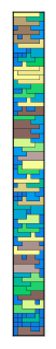
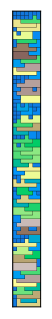
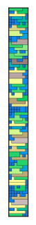
Figure 3. Five random ${n\times 7}$ tillings of areas in the interval $[500;520]$ using in total $95$ different tiles.

Let us remark that we need to approximate the control vector $\hat{x}$ with precision of order $O(\frac{1}{n})$ to obtain a rejection sampler with linear time complexity. For a more detailed analysis we invite the curious reader to (bendkowski_bodini_dovgal_2021).

4. Architecture overview

With the tuning as convex optimisation principle we can tune the control vector and obtain a Boltzmann model realising the user-declared values. Given a system such as

⬇

mkBoltzmannSampler

System

{ targetType = ”Lambda

, meanSize = 10_000

, frequencies = (’Abs, 4_000) <:> def

, weights =

(’Index, 0)

<:> $(mkDefWeights ”Lambda)

}

the presented framework must

• compute the control vector parameters and related generating function values for the user-declared parameter values, and

• compile a Boltzmann sampler realising the computed Boltzmann model.

These steps involve a series of intermediate transformations which are organised through a stack of embedded domain specific languages, spread across our Haskell prototype and the Python tuner paganini. In the following sections we outline some of the key features of these transformations.

4.1. Computing constructor distributions

To compute the required control vector and generating function values, we convert the system declaration into a paganini input using a custom monadic eDSL we call paganini-hs. It is meant as a thin Haskell wrapper around paganini, providing a convenient and type safe way of expressing the tuning problem.

⬇

formProblem ::

IO (Either PaganiniError [Maybe Double])

formProblem = paganini’ @@ do

Let z <- variable’ 10_000

Let u <- variable’ 4_000

\parLet d <- variable

Let l <- variable

\par– $D(z,u) = z + z D(z,u)$

d .=. z + z * d

\par– $L(z,u) = D(z, u) + z {L(z, u)}^{2} + z u L(z, u)$

l .=. d + z * l^2 + z * u * l

\partuneAlgebraic l – tune for l

value <$> [z, u, l, d]

We start with introducing two marking variables

z} and
\mintinline[fontsize=\small]

haskellu which correspond to the size of generated lambda terms and the number of their abstractions, respectively. These variables are initialised with user-declared values. Next, we introduce two more variables

d} and
\mintinline[fontsize=\small]

haskelll which correspond to $L(z,u)$ and $D(z,u)$, respectively. Note that these variables are not tuned. Next, we proceed with mapping type definitions to their corresponding generating function definitions following the symbolic method outlined in subsection 3.1. For each type, we provide its defining equation using the

(.=.)} operator
\begin

minted[escapeinside=——,mathescape=true,fontsize=]haskell (.=.) :: Variable -¿ Expr -¿ Spec () Note that on one hand side, we want to conveniently use variables to build more involved expressions while on the other hand, we do not want expressions to be used on the left-hand sides of defining equations. Hence, to lift variables into expressions we use existential types in the definition of

Let}:
\begin

minted[escapeinside=——,mathescape=true,fontsize=]haskell newtype Let = Let (forall a . FromVariable a =¿ a) class FromVariable a where fromVariable :: Variable -¿ a instance FromVariable Let where … instance FromVariable Exp where … Now, it is possible to safely use variables in the contexts permitting expressions while keeping Variable}s and \mintinline[fontsize=\small]haskellExps logically separated. Once the definitions of the type variables are defined, we invoke paganini using

tuneAlgebraic l}, and output
the tuned values of $z, u, L(z,u), D(z,u)$.
The whole computation is expressed in a specification monad
\mintinline[fontsize=\small]

haskellSpec which formulates a corresponding problem in the input format of paganini:

⬇

import paganini as pg

spec = pg.Specification()

z = pg.Variable(10000)

d = pg.Variable(4000)

l = pg.Variable()

d = pg.Seq(z)

\parspec.add(l, d + z * u * l + z * l**2)

spec.run_tuner(l, method = pg.Method.STRICT)

\parprint (z.value)

print (u.value)

print (l.value)

print (d.value)

The

Spec} monad is a simple state
transformer monad
\begin

minted[escapeinside=——,mathescape=true,fontsize=]haskell type Spec = StateT Program IO letting us compose a dedicated paganini

Program} and
execute it by an external Python interpreter.  Afterwards, the program result,
\emph

i.e. the tuning variable values, are collected and returned back as a Haskell level value. Let us notice that paganini itself is a python DSL written on top of CVXPY (diamond2016cvxpy) — a modelling library and de facto eDSL for disciplined convex optimisation. It lets us express the tuning problem in a convenient, domain specific form which can be then transformed into a readily solvable convex optimisation problem. Note that in doing so, our framework does not need to formulate the problem directly, but rather can treat paganini as a black-box solver. Finally, let us notice that we retain the original variable names while composing the paganini program using a source code reification library BinAnn (10.1007/978-3-030-57761-2_2). Variables names are reflected in both DSLs. Such a design choice makes debugging easier and lets paganini-hs provide better error messages with meaningful variable names.

4.2. Sampling from discrete distributions

Once the values of the control vector and corresponding generating functions are computed, we can readily calculate the branching probabilities for involved types. Recall that for a type

a}, the
respective Boltzmann sampler for \mintinline[fontsize=\small]

haskella has to make a random decision determining which constructor to use in the process of generating a random object in

a}. In our
running example, the \emph

branching probabilities for type

Lambda}
take the form
\begin

equation D(z,u)L(z,u)  z u L(z,u)L(z, u)  z L(z, u)2L(z,u) for Index}, \mintinline[fontsize=\small]haskellAbs, and

Abs}, respectively, and aptly chosen values of $z$ and $u$.
Hence, in order to choose a constructor
we have to draw a random variable from a \emph

(finite) discrete probability distribution. To do so, we can resort to the well-known inversion method (Devr86); we partition the interval $[0,1]$ into three segments, each of length corresponding to one of the available constructors, draw a random real $p$ in between zero and one, and determine in which segment does $p$ fall into. While it is possible to choose random constructors using the inversion scheme, let us remark that it is quite inefficient for our application. The inversion method works well under the (unrealistic) real RAM model in which we operate on real numbers. In practice, we do not have arbitrary precision real numbers, but rather finite precision floating-point numbers. The inversion scheme samples therefore a random double-precision floating point number $p\in[0,1]$ to select one of the distribution points. In some cases the available precision of a single floating-point number might be not enough. In others, fewer bits are sufficient. For instance, note that in order to sample from a distribution $\left(\frac{1}{2},\frac{1}{2}\right)$ a single bit is sufficient. Due to these limitations, we do not use the inversion scheme but rather resort to a different approach following the random bit model of sampling introduced by Knuth and Yao in (KY76). Instead of using a single floating-point number to sample from a discrete distribution, one accesses a lazy stream of random bits, consuming one bit at a time. These bits are then used to refine the search space until a single value can be chosen. For performance reasons, in our implementation we do not use an actual stream of bits, but rather use a buffered oracle, as suggested in (DBLP:journals/corr/abs-1304-1916).

⬇

data Oracle g = Oracle

{ buffer :: !Word32

, usedBits :: !Int

, rng :: g

}

The oracle type

Oracle g} is parameterised
by a random number generator \mintinline[fontsize=\small]

haskellg. The oracle consists of a 32-bit buffer and a counter keeping track of how many random bits have been consumed so far from the current buffer. If the buffer gets depleted, it can be regenerated as follows

⬇

fresh :: RandomGen g => g -> Oracle g

fresh g = case random g of

(x, g’) -> Oracle { buffer = x

, usedBits = 0

, rng = g’

}

Using the

Oracle} type, we can now define
a \mintinline[fontsize=\small]

haskellBuffonMachine monad for random computations in the random bit model framework. The

BuffonMachine} type is implemented as a
\mintinline[fontsize=\small]

haskellnewtype wrapper around the

State} monad:
\begin

minted[fontsize=]haskell newtype BuffonMachine g a = MkBuffonMachine runBuffonMachine :: State (Oracle g) a deriving (Functor, Applicative, Monad) via State (Oracle g) Using the ideas of (KY76) it is possible to construct an entropy-optimal discrete distribution-generating tree (DDG) implementing a sampler for any discrete distribution $P$ of rational numbers. In other words, it is possible to construct a sampler for $P$ which uses the least average number of random bits to sample from $P$. Unfortunately, the entropy-optimal DDGs can be exponentially large in the number of bits required to encode the input distribution $P$. For instance, the binomial distribution $\mathbb{B}(n,p)$ with parameters $n=50$ and $p=\frac{61}{500}$ requires a DDG of height $10^{104}$, see (10.1145/3371104). Unfortunately, such an overhead renders DDGs virtually impractical. Due to that, we use recently developed approximate sampling schemes (10.1145/3371104) which are a practical trade-off between the entropy perfect DDGs and feasible, finite precision sampling algorithms. Instead of sampling from a discrete probability distribution $P=(p_{1},\ldots,p_{n})$ we find an entropy optimal sampling algorithm for a closest approximation $\hat{P}=(\hat{p}_{1},\ldots,\hat{p}_{n})$ of $P$ among all sampling algorithms which operate within a finite $k$-bit precision. Let us note that the framework of approximate sampling schemes, and in particular its prototype implementation, supports several statistical measures of approximation error between probability distributions, including Kullback-Leibler, Pearson chi-square, and Hellinger divergence. The optimal approximate distribution $\hat{P}$ can be readily found as soon as the constructor distribution is computed in so-called linear, compact vector form. We use a prototype implementation of optimal approximate sampling algorithms to find the compact vector form of DDGs. Compiled Boltzmann samplers readily choose constructors from the compact DDGs represented as

Vector Int}.
\subsection

Anticipated rejection A straightforward implementation of Boltzmann samplers

⬇

sample :: RandomGen g => BuffonMachine g a

has some practical drawbacks. While the underlying Boltzmann model provides control over the mean size of its outcomes, we have no finer control over the actual size of generated objects. In some cases, the outcome sample size might be significantly larger than the user-declared mean size. Without any additional control, Boltzmann samplers might consume significantly more resources than required. In the presented framework we implement Boltzmann samplers with anticipated rejection, see (BodGenRo2015). The idea is quite simple. The user provides an upper bound on the size of generated outcomes. During generation we maintain the current size of the sample. If it exceeds the given upper bound, the process is terminated and the sample is rejected. Consequently, the signature of

sample} becomes
\begin

minted[fontsize=]haskell sample :: RandomGen g =¿ UpperBound -¿ MaybeT (BuffonMachine g) (a, Int) To give the user a more fine-grained control over the outcome size of sampled objects, the user can provide an admissible size range $[(1-\varepsilon)n,(1+\varepsilon)]$. The framework samples objects until one with admissible size is generated. Note that such a rejection scheme guarantees that inadmissible samples are rejected as soon as possible.

⬇

toleranceRejectionSampler ::

(RandomGen g, BoltzmannSampler a) =>

MeanSize -> Double -> BuffonMachine g a

toleranceRejectionSampler n eps =

rejectionSampler lb ub

where

lb = MkLowerBound $

floor $ (1 - eps) * fromIntegral n

ub = MkUpperBound $

ceiling $ (1 + eps) * fromIntegral n

Let us remark that anticipated rejection has an tiny impact on the underlying Boltzmann model. As we limit admissible sizes, we also impose a small bias in the distribution, initially not taken into account. Indeed, objects of inadmissible sizes can no longer be sampled, and so their total probability mass gets redistributed among admissible objects. In consequence, the original tuning goal $\mathbb{E}(N)=n$ must be modified to accommodate an additional bias parameter $\delta$ such that $\mathbb{E}(N)=\delta n$, cf. (bendkowski_bodini_dovgal_2021). The specific value of $\delta$ depends on the type of parameter corresponding to the variable $N$ and, in particular, its corresponding asymptotic behaviour in the related system of multivariate generating functions. While our prototype implementation does not introduce the bias parameter, let us remark that it can diminish the overall number of rejections required to find an admissible sample. For more details we invite the curious reader to (bendkowski_bodini_dovgal_2021).

4.3. ADT and newtype samplers

Boltzmann samplers for algebraic data structures have a regular format. For instance, our running example of

Lambda}
has the following\footnote

For the reader’s convenience, we elide boilerplate code which clouds the structure of the algorithm. Boltzmann sampler:

⬇

instance BoltzmannSampler Lambda where

sample ub =

do guard (ub >= 0)

lift (BuffonMachine.choice …)

>>=

(\case0 -> do (x_0, w_0) <- sample ub

pure (Index x_0, w_0)

1 -> do (x_0, w_0) <- sample (ub - 1)

(x_1, w_0) <- sample (ub - w_0 - 1)

pure (App x_0 x_1, 1 + w_0 + w_1)

2 -> do (x_0, w_0) <- sample (ub - 1)

pure (Abs x_0, 1 + w_0)

The

sample} function has a single
parameter \mintinline[fontsize=\small]

haskellub which defines a size budget which the sampler cannot overreach, as enforced by

guard (ub >= 0)}.
If the sampler has some non-negative size budget left, it can proceed with
generating the object. To do so, the sampler draws a random
number according to the respective constructor distribution.
The choice function has signature
\begin

minted[fontsize=]haskell choice :: RandomGen g =¿ Distribution -¿ Discrete g where

⬇

newtype Distribution =

MkDistribution {unDistribution :: Vector Int}

deriving stock (Show)

\partype Discrete g = BuffonMachine g Int

represent the compact linear DDG, and discrete random integer variables. Note that the actual distribution is inserted directly in the body of the sampler function. Next, the generated random number is mapped onto a concrete constructor. We use

sample} to generate all of the constructor
parameters. At the same time, we keep track of the size budget accounting for
the weight of the considered constructor and size of each generated
subexpression.
Such a Boltzmann sampler construction easily generalises onto arbitrary
algebraic data types. However, since samplers are implemented as instances of
the \mintinline[fontsize=\small]

haskellBoltzmannSampler type class, we can have at most one sampler for each type. In some circumstances, we might want to have multiple samplers for the same type. To support such use cases, we support the compilation of Boltzmann samplers for

newtype} synonyms.  Note that the
structure of such Boltzmann samplers is \emph

almost