50 shades of Bayesian testing of hypotheses

Abstract

Hypothesis testing and model choice are quintessential questions for statistical inference and while the Bayesian paradigm seems ideally suited for answering these questions, it faces difficulties of its own ranging from prior modelling to calibration, to numerical implementation. This chapter reviews these difficulties, from a subjective and personal perspective.

Keywords: Bayesian model selection, BIC, DIC, Hypothesis testing, Improper priors, Information criterion, Mixtures, Monte Carlo, Posterior predictive, Prior specification, WAIC.

1 Introduction

The concept of hypothesis testing is somewhat inseparable from statistics as principled hypothesis testing is unfeasible outside a statistical framework, while testing may be the most ubiquitous and long-standing manifestation of statistical practice, if not in theoretical statistics. The implementation of this goal is also subject to many interpretations and controversies, as illustrated by the recent American Statistical Association statement on the dangers of over-interpreting $p$-values (Wasserstein and Lazar, , 2016) and other calls (Johnson, , 2013; Gelman and Robert, , 2014; Benjamin et al., , 2018; McShane et al., , 2019). In particular, testing is a dramatically differentiating feature separating classical from Bayesian paradigms, both conceptually and practically Berger and Sellke, (1987); Casella and Berger, (1987). This opposition will not be covered by the present chapter.

Even within the Bayesian community, testing hypotheses remains an area that is wide open to controversy and divergent opinions, from banning any form of testing to constructing pseudo-$p$-values. While the notion of the posterior probability of an hypothesis appears as a “natural” answer in a Bayesian context, there exist many issues with that choice, from the impact of the prior modelling to the impossibility of using improper priors, as shown by the Jeffreys-Lindley paradox Lindley, (1957); Robert, 2014a . Furthermore, the most common binary (i.e., accept vs. reject) outcome of an hypothesis test appears more suited for immediate decision (if any) than for model evaluation, clashing with the all-encompassing nature of Bayesian inference.

The literature on Bayesian hypothesis testing is huge and we can only point out to a few significant entries like Berger, (1985); Gelman et al., (2013); Vehtari and Ojanen, (2012); Gelman et al., (2014). The in-depth analysis of Harold Jeffreys’ input by Ly et al., (2016) is quite noteworthy.

2 Bayesian hypothesis testing

“In induction there is no harm in being occasionally wrong; it is inevitable that we shall be. But there is harm in stating results in such a form that they do not represent the evidence available at the time when they are stated.” — Harold Jeffreys (1939)

As a preliminary, let me point out that Bayesian hypothesis testing (or model selection, as I will use both terms interchangeably) can be seen as a comparison of $k>1$ potential statistical models towards the selection of the model that fits the data “best”. A mostly accepted perspective is indeed that it does not primarily seek to identify which model is “true”, but compares fits through marginal likelihoods or other quantities.

A marginal likelihood (or evidence) is defined as the average likelihood function

$$m(x)=\int_{\Theta}L(\theta|x)\pi(\theta)\,\text{d}\theta$$

where $L(\theta|x)$ denotes the likelihood function attached to the sample $x$, $\pi(\cdot)$ is the prior density and $\Theta$ the parameter space. This quantity naturally includes a penalisation addressing model complexity and over-fitting, through the averaging over the whole set $\Theta$, that is mimicked by Bayes Information (BIC) (Schwartz, , 1965; Schwarz, , 1978) and Deviance Information (DIC) criteria (Spiegelhalter et al., , 2002; Plummer, , 2008). A fundamental difficulty with the marginal likelihood is that it exhibits a long-lasting impact of prior modeling, in that the likelihood input does not quickly counter-balance the tail behaviour of the prior.

Each model (or hypothesis) $\mathcal{M}_{i}$ under consideration comes with an attached triplet $(L_{i}(\cdot|x),\pi_{i}(\cdot),\Theta_{i})$ $(i=1,\ldots,k)$. In addition, prior weights $\omega_{i}$ are characterising the prior probabilities of the models, leading to an encompassing prior

$$\pi(\theta)=\omega_{1}\pi_{1}(\theta)\mathbb{I}_{\Theta_{1}}(\theta)+\cdots+\omega_{k}\pi_{k}(\theta)\mathbb{I}_{\Theta_{k}}(\theta)$$

and the corresponding posterior probabilities

$$\pi(\mathcal{M}_{i}|x)=\dfrac{\omega_{i}\int_{\Theta_{i}}L_{i}(\theta_{i}|x)\pi_{i}(\theta_{i})\,\text{d}\theta_{i}}{\sum_{j=1}^{k}\int_{\Theta_{j}}\omega_{j}L_{j}(\theta_{j}|x)\pi_{j}(\theta_{j})\,\text{d}\theta_{j}}=\dfrac{m_{i}(x)}{\sum_{j=1}^{k}m_{j}(x)}$$

A decision-theoretic approach based on the Neyman-Pearson formalism of hypothesis testing leads to selecting the most probable model (Berger, , 1985; Lehmann, , 1986). However, the strong impact of the values of the prior weights $\omega_{i}$ on the numerical values of these posterior probabilities led to their removal and the construction of the Bayes factors (Wrinch and Jeffreys, , 1919; Haldane, , 1932; Jeffreys, , 1939), comparing the marginal likelihoods between models $(L_{i},\pi_{i})$ and $(L_{j},\pi_{j})$ by the ratio

$$\mathfrak{B}_{ij}=\dfrac{\int_{\Theta_{i}}L_{i}(\theta_{i}|x)\pi_{i}(\theta_{i})\,\text{d}\theta_{i}}{\int_{\Theta_{j}}L_{j}(\theta_{j}|x)\pi_{j}(\theta_{j})\,\text{d}\theta_{j}}$$ (1)

which amounts to selecting among models the model with the highest marginal. This is also advocated as an even weighting of both models in Jeffreys, (1939), but I see little justification for this choice, especially when considering multiple model selection with possibly embedded models.

The coexistence of both notions—posterior probability versus Bayes factor—exhibits a tension between using (i) posterior probabilities as justified by binary loss functions but depending on subjective prior weights that prove difficult to specify in most settings, especially when comparing many hypotheses, and (ii) Bayes factors that eliminate this dependence but escape a direct connection with a posterior distribution, unless the prior weights are themselves integrated within the loss function. A further difficulty attached to the Bayes factors is that they face a delicate interpretation (or calibration) of the strength of their support of a given hypothesis or model, even when shown to be consistent in the sample size (Berger et al., , 2003; Dass and Lee, , 2006), as illustrated by Figure 1. That is, under fairly generic conditions on the priors, the Bayes factor $\mathfrak{B}_{ij}$ will diverge to infinity or to zero when the sampling model is $\mathfrak{M}_{i}$ or $\mathfrak{M}_{j}$, respectively, as the sample size grows to infinity (Chib and Kuffner, , 2016; O’Hagan, , 1997; Johnson, , 2008; Moreno et al., , 2010). The differentiation between the simulated values of the Bayes factors under the null model and under the alternative model is getting more pronounced in this figure as the sample size grows. As functions of the data $x$, both notions are such that their calibration and a necessary variability assessment seem to require (frequentist or posterior predictive) simulations under both hypotheses, which clashes with the Bayesian paradigm. However, posterior probabilities face a similar difficulty if one wants to avoid interpreting them as $p$-value substitutes or probabilities of selecting the “true” model. since they only report of respective strengths of fitting the data $x$ to the models under comparison.

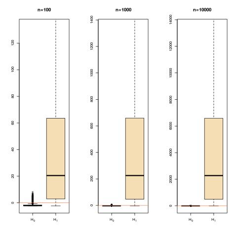
Figure 1: Example of a normal ${\bar{X}}_{n}\sim\mathcal{N}(\mu,\nicefrac{{1}}{{n}})$ model when $\mu\sim\mathcal{N}(0,1)$ under $H_{1}$ and $\mu=0$ under $H_{0}$, leading to the Bayes factor $\mathfrak{B}_{10}=(1+n)^{-\nicefrac{{1}}{{2}}}\exp\{n^{2}{\bar{x}}^{2}_{n}/2(1+n)\}$. The three panels represent the variability of $\log\mathfrak{B}_{10}$ over 250 replicas under the null (left) and the alternative (right) hypotheses, for three different sample sizes $n$. In the later case, the replications are generated from the prior predictive distribution. This experiment is supporting the statement about the consistency of the Bayes factor, namely that the true model is selected by the Bayes factor when the sample size $n$ goes to infinity, since the Bayes factor $\mathfrak{B}_{10}$ accumulates at zero under $H_{0}$ and diverges under $H_{1}$.

“Bayes factors also suffers from several theoretical and practical difficulties. First, when improper prior distributions are used, Bayes factors contains undefined constants and takes arbitrary values (…) Second, when a proper but vague prior distribution with a large spread is used to represent prior ignorance, Bayes factors tends to favour the null hypothesis. The problem may persist even when the sample size is large (…) Third, the calculation of Bayes factors generally requires the evaluation of marginal likelihoods. In many models, the marginal likelihoods may be difficult to compute.” – Yong Li, Tao Zen, and Jun Yu (2014)

Among other difficulties inherent to the use of the Bayes factor, and as illustrated by the above quote, let me mention an impossibility to ascertain simultaneous misfits to all proposed models (unless a non-parametric alternative is added as in Holmes et al., , 2015) or to detect outliers, that is a subset of the dataset that does not fit a particular model. Another pressing issue I will not address here is the challenging numerical computation of marginal likelihoods in most settings. While numerous proposals have been made (see, e.g., Chen et al., , 2000; Robert and Casella, , 2004; Chopin and Robert, , 2010; Friel and Pettitt, , 2008; Robert and Marin, , 2008; Marin and Robert, , 2011; Friel and Wyse, , 2012), there is no universal solution and new settings require a careful design of the numerical apparatus producing the evidence. A last difficulty worth pointing out is the strong dependence of posterior probabilities and Bayes factors on conditioning statistics, which undermines their validity for model assessment. This issue was exhibited when considering ABC (Approximate Bayesian computation, see Sisson et al., , 2018) model choice as the lack of inter-model sufficiency may drastically alter the value of a Bayes factor and even its consistency (Didelot et al., , 2011; Robert et al., , 2011; Marin et al., , 2014).

3 Improper priors united against hypothesis testing

Hypothesis testing sees a glaring discontinuity occur in the valid use of improper (infinite mass) priors since calling on these is not directly justified in most testing situations, leading to many alternative and ad hoc solutions, where data is either used twice or split in artificial ways. This is most unfortunate in that the remainder of Bayesian analysis accommodates rather smoothly the extension from proper (that is, true probability) prior distributions to improper (that is, $\sigma$-finite) prior distributions, which is in particular most helfpul in closing the range of Bayesian procedures. The fundamental reason for the difficulty in the testing context is the necessity to define a prior distribution for each model under comparison, independently of the other priors. This means there is no rigorous way of defining a model-by-model normalisation of these priors when they are $\sigma$-finite. (Principled constructions of reference priors for testing have been investigated, see for instance Bayarri and García-Donato, , 2007 and Bayarri and García-Donato, , 2008. Their proposal is based on symmetrised versions of the Kullback-Leibler divergence $\kappa$ between the null and alternative distributions, transformed into a prior that looks like an inverse power of $1+\kappa$, with a power large enough to make the prior proper.)

A first difficulty with the proposed resolutions of the improper conundrum stands with the choice (already found in Jeffreys, , 1939) of opting for identical priors on the parameters present in both models (Berger et al., , 1998), which amounts in endowing them with the same meaning. The following argument of then using the same prior, whether or not proper, then eliminates the need for a normalising constant. (Note that the Savage–Dickey approximation of the marginal likelihood relies on this assumption and operates only under the alternative hypothesis, see Verdinelli and Wasserman, , 1995; Marin and Robert, , 2010.)

A second difficulty is attached to the pseudo-Bayes factors proposed in the 1990’s (O’Hagan, , 1995; Berger et al., , 1998), where a fraction of the data is used to turn all improper priors into proper posteriors and these posteriors are used as new “priors” on the remaining fraction. On the one hand this is a nice bypass of the normalisation constant issue and it enjoys consistency properties as the sample size of the remaining fraction grows to infinity. Furthermore, it does not use the data twice as (Aitkin, , 1991, 2010). On the other hand, being a leave-one-out approach, it does not qualify as a Bayesian procedure proper and the different manners to average over all possible choices of the normalising sample lead to different numerical answers, while there exist cases when this division proves impossible.

Alternative approaches have advocated the use of score functions (Hyvärinen, , 2005; Gutmann and Hyvärinen, , 2012; Li et al., , 2014; Dawid and Musio, , 2015; Shao et al., , 2017) to overcome the issue with improper priors. While quite sympathetic to this perspective, I will not cover this aspect in this chapter.

While the deviance information criterion (DIC) of (Spiegelhalter et al., , 2002, 2014) remains quite popular for model comparison, its uses of the posterior expectation of the log-likelihood function, meaning that the data is used twice, as in Aitkin, (2010), and of a plug-in term, make it disputable, as discussed in Robert, 2014b and prone to conflicting interpretations, as shown in Celeux et al., (2006) for mixtures of distributions. A related approach with stronger theoretical backup is the widely applicable information criterion (WAIC) of Watanabe, (2010, 2018), which is asymptotically equivalent to the average Bayes generalization and cross validation losses. The fundamental setting of WAIC is one where both the sampling and the prior distributions are different from respective “true” distributions. This requires using a tool towards the assessment of the discrepancy when utilising a specific pair of such distributions, especially when the posterior distribution cannot be approximated by a Normal distribution. The WAIC is supported for the determination of the “true” model, in opposition to AIC and DIC. In addition, it escapes the “plug-in” sin and is handling mixture models.

4 The Jeffreys–Lindley paradox

“The weight of Lindley’s paradoxical result (…) burdens proponents of the Bayesian practice”. – Frank Lad (2003)

The Lindley paradox (or Jeffreys–Lindley paradox) is due to Lindley, (1957) pointing out an irreconciliable divergence between the classic and Bayesian procedures when testing a point null hypothesis. (This property was briefly mentioned in Jeffreys, , 1939, V, §5.2, although in their scholarly review of the paradox, Wagenmakers and Ly, , 2021 stress that it plays a central role in his construction of Bayesian hypothesis testing.) The paradox is that, regardless of the prior choice, the Bayes factor against the null hypothesis converges to zero with the sample size when the associated $p$-value remains constant. For instance, when testing the nullity of a Normal mean,

$$\bar{x}_{n}\sim\mathcal{N}(\theta,\sigma^{2}/n)\,,\quad H_{0}:\,\theta=\theta_{0}\,,$$

with the following $H_{1}$ prior, $\theta\sim\mathcal{N}(\theta_{0},\sigma^{2})$, the Bayes factor is

$$\mathfrak{B}_{01}(t_{n})=(1+n)^{1/2}\,\exp\left(-nt_{n}^{2}/2[1+n]\right)\,,$$

where $t_{n}=\sqrt{n}|\bar{x}_{n}-\theta_{0}|/\sigma$. When setting $t_{n}$ to a fixed value, it converges to infinity with $n$.

“ The Jeffreys–Lindley paradox exposes a rift between Bayesian and frequentist hypothesis testing that strikes at the heart of statistical inference.” – Eric-Jan Wagenmakers and Alexander Ly (2021)

Since the apparent paradox of “always” accepting the null hypothesis can be reformulated in terms of a prior variance going to infinity, it also relates with the difficulty in using Bayes factors and improper priors, in that the posterior mass of the region with non-negligible likelihood goes to zero as the variance increases (Robert, 2014c, ). This is thus a coherent framework in that the only remaining item of information is that the null hypothesis could be true! (Note also that the paradox can be circumvoluted by replacing the point null hypothesis with an interval substitute in order for a single proper or improper prior to be used, see also Robert, , 1993.)

The opposition between frequentist and Bayesian procedures is not a surprise either. The former relies solely on the point-null hypothesis $H_{0}$ and the corresponding sampling distribution, while the latter opposes $H_{0}$ to a (predictive) marginal version of $H_{1}$. Furthermore, the fact that the statistic $t_{n}$ remains constant (or equivalently that the Type I error remains constant) is incorrect. The rejection bound cannot be a constant multiple of the standard error as the sample size $n$ increases, as demonstrated by Jeffreys, (1939) and discussed in details by Wagenmakers and Ly, (2021). Let me conclude by mentioning the case for specific priors isolating the null from the alternative hypotheses, as in Consonni and Veronese, (1987); Johnson and Rossell, (2010) and Consonni et al., (2013).

5 Posterior predictive $p$-values

Once a Bayes factor $\mathfrak{B}_{01}$ is computed, one need assess its strength in supporting one of the hypotheses, if any. In my opinion, the much vaunted Jeffreys’ (1939) scale has very little validation as it is absolute (i.e., with no dependence on the model, the sample size, the prior). Following earlier proposals in the literature (Box and Tiao, , 1992; García-Donato and Chen, , 2005; Geweke and Amisano, , 2008), an evaluation of this strength within the issue at stake, i.e., the comparison of two hypotheses (or models), can be based on the predictive distributions. That is, the likelihood of observing $\mathfrak{B}_{01}(x^{\text{obs}})$, the observed dataset, is evaluated under these distributions

$$\mathbb{P}_{0}^{\text{pred}}(\mathfrak{B}_{01}(X^{\text{pred}})\geq\mathfrak{B}_{01}(x^{\text{obs}})|x^{\text{obs}})$$

and

$$\mathbb{P}_{1}^{\text{pred}}(\mathfrak{B}_{01}(X^{\text{pred}})\leq\mathfrak{B}_{01}(x^{\text{obs}})|x^{\text{obs}})$$

the probabilities being computed under models $\mathfrak{M}_{0}$ and $\mathfrak{M}_{1}$, respectively.

While most authors (like García-Donato and Chen, 2005) consider this should be the prior predictive distribution, I agree with Gelman et al., (2013) that using the push-forward image by $\mathfrak{B}_{01}(\cdot)$ of the posterior predictive distribution

$$\pi(x^{\text{rep}}|x^{\text{obs}})=\int p(x^{\text{rep}}|\theta)\pi(\theta|x^{\text{obs}})\,\text{d}\theta$$ (2)

(where $x^{\text{obs}}$ denotes the observed dataset and $x^{\text{rep}}$ an artificial replication or a running variate) is more relevant. Indeed, by exploiting the information contained in the data (through the posterior), (2) concentrates on a region of relevance in the parameter space(s), which is especially interesting in weakly informative settings, despite “using the likelihood twice”. Furthermore, (2) evaluate the behaviour of the Bayes factor for values of $x$ that are similar to the original observation, provided the posterior predictive fits the data well enough. Note also that, under this approach, issues of indeterminacy linked with improper priors are not evacuated, since the Bayes factor remains indeterminate, even with a well-defined predictive. Note further that, even though probabilities of errors of type I and errors of type II can be computed, they fail to account for the posterior probabilities of both models. (This is a potentially delicate issue with the solution of García-Donato and Chen, 2005.) A nice feature is that the predictive distribution of the Bayes factor can be computed even in complex settings when ABC (Sisson et al., , 2018) need be used.

“If the model fits, then replicated data generated under the model should look similar to the observed data. The observed data should look plausible under the posterior predictive distribution. This is really a self-consistency check: an observed discrepancy can be due to model misfit or chance.” – Andrew Gelman et al. (2013)

In Bayesian Data Analysis (2013, Chapter 6), based on the choice of a measure of discrepancy $T(\cdot,\cdot)$, the authors (strongly) suggest replacing the classical $p$-value

$$p(x^{\text{obs}}|\theta)=\mathbb{P}(T(X^{\text{rep}},\theta)\geq T(x^{\text{obs}},\theta)|\theta)$$

with a Bayesian alternative (or Bayesian posterior $p$-value)

$$\mathbb{P}(T(X^{\text{rep}},\theta)\geq T(x^{\text{obs}},\theta)|x^{\text{obs}})\,.$$

Extremes $p$-values indicate a poor fit of the model, with the usual caution applying about setting golden bounds such as $0.05$ or $0.99$. There are however issues with the implementation of this approach, from deciding on which aspect of the data or of the model is to be examined, i.e., the choice of the discrepancy measure $T$, to its calibration.

6 A modest proposal

Given this rather pessimistic perspective on Bayesian testing, one may wonder at the overall message of this chapter besides the not-particularly useful “it is complicated”. Given the difficulty in moderating the impact of the prior modelling in ways more useful than a sheer assurance of consistency, my preference leans towards a proposal that feels more estimation-based than testing-based, and that is leaning more towards quantification than towards binary decision. In Kamary et al., (2014), we have sketched the basis of a novel approach that advocates the replacement of the posterior probability of a model or of an hypothesis with the posterior distribution of the weights of a mixture of the models under comparison. That is, given two Bayesian models under comparison,

$$\mathfrak{M}_{1}:x\sim f_{1}(x|\theta_{1})\,,\theta_{1}\sim\pi_{1}(\theta_{1})\text{ versus }\mathfrak{M}_{2}:x\sim f_{2}(x|\theta_{2})\,,\theta_{2}\sim\pi_{2}(\theta_{2})$$

we propose to estimate the (artificial) mixture model

$$\mathfrak{M}_{\alpha}:x\sim\alpha f_{1}(x|\theta_{1})+(1-\alpha)f_{2}(x|\theta_{2})\quad 0\leq\alpha\leq 1$$ (3)

and in particular to derive the posterior distribution of $\alpha$. This (marginal) posterior can then be exploited to assess the better fit and if need be to achieve a decision, either by assessing tail probabilities that $\alpha$ is close to $0$ or $1$, or by calibrating a bound from the prior or posterior predictives. In most settings, this approach can indeed be easily calibrated by a parametric bootstrap experiment providing a posterior distribution of $\alpha$ under each of the models under comparison. The prior predictive error can therefore be directly estimated and drive the choice of a decision cut-off on the tails of $\alpha$, if need be.

Consider for instance a simple example in Kamary et al., (2014) where $f_{1}(\cdot|\theta_{1})$ corresponds to a Poisson $\mathcal{P}(\theta_{1})$ distribution and $f_{2}(\cdot|\theta_{1})$ to a Geometric $\mathcal{G}eo(\theta_{2})$ failure distribution, both parameterised in terms of their mean. A mixture

$$\alpha\mathcal{P}(\lambda)+(1-\alpha)\mathcal{G}eo(\nicefrac{{1}}{{1+\lambda}})$$

can then be proposed, with the same parameter $\lambda>0$ behind both components. Further, Kamary et al., (2014) show that the non-informative prior $\pi(\lambda)=\nicefrac{{1}}{{\lambda}}$ can be used in this setting, whatever the sample size $n$. Figure 2 demonstrates the concentration of the posterior on $\alpha$ around $1$ as $n$ increases when the data generating distribution is a $\mathcal{P}(\lambda)$ distribution.

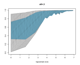
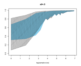
Figure 2: Posterior means (sky-blue) and medians (grey-dotted) of the posterior distributions on $\alpha$, displayed over $100$ simulations of Poisson $\mathcal{P}(4)$ datasets for sample sizes $n$ between 1 and 1000. The shaded and dotted areas indicate the range of the estimates. Each plot corresponds to a $\mathcal{B}e(a_{0},a_{0})$ prior on $\alpha$ and each posterior approximation is based on $10^{4}$ MCMC iterations. This experiment is supporting the statement about the concentration of the posterior on the mixture weight near the upper limit $1$, in agrement with the correct model. (Source: Kamary et al., , 2014)

In this example, the exact (standard) Bayes factor comparing the Poisson to the Geometric models is given by

$$\mathfrak{B}_{12}=n^{n\bar{x}_{n}}\prod_{i=1}^{n}x_{i}!\,{\Gamma\left(n+2+n\bar{x}_{n}\right)}\big{/}{\Gamma(n+2)}.$$

when using the same improper prior on the parameter $\lambda$ (DeGroot, , 1973, 1982; Berger et al., , 1998). The posterior probability of the Poisson model is then derived as

$$\mathbb{P}(\mathfrak{M}_{1}|x)=\frac{\mathfrak{B}_{12}}{1+\mathfrak{B}_{12}}$$

when adopting (without much of a justification) identical prior weights on both models. Figure 3 compares the concentration of the posterior probabiliy and of the posterior median on $\alpha$ around $1$ as $n$ increases.

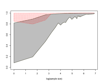
Figure 3: Comparison between the ranges of $\mathbb{P}(\mathfrak{M}_{1}|x)$ (red dotted area) and of the posterior medians of $\alpha$ for $100$ simulations of Poisson $\mathcal{P}(4)$ datasets with sample sizes $n$ ranging from $1$ to $10^{3}$. (Source: Kamary et al., , 2014)

One may object that the mixture model (3) is neither one nor the other of the models under comparison, but it includes both of these at the boundaries, i.e., when $\alpha=0,1$. Thus, if we use a prior distribution on $\alpha$ that favours neighbourhoods of $0$ and $1$, albeit avoiding atoms at these values, we should be able to witness the posterior concentrate near $0$ or $1$, depending on which model is true (or fits the data better). This is indeed the case: as shown in Kamary et al., (2014), for any given Beta prior on $\alpha$, we observe a higher and higher concentration at the right boundary as the sample size $n$ increases, as illustrated by Figure 2.

In our opinion, this (novel) mixture approach offers numerous advantages. First, achieving a decision while relying on a Bayesian estimator of the weight $\alpha$ or on its posterior distribution, rather than on the posterior probability of the associated model lifts the embarassing need of specifying almost invariably artificial prior probabilities on the models, as discussed above. This is also a most Bayesian choice, replacing an unknown quantity with a probability distribution. It is however not addressed by a classical Bayesian approach, even though those probabilities linearly impact the posterior probabilities and their indeterminacy is often brought forward to promote the alternative of using instead the Bayes factor. In the mixture estimation setting, prior modelling only involves selecting a prior on $\alpha$, for instance a Beta $\mathcal{B}(a,a)$ distribution, with a wide range of acceptable values for the hyperparameter $a$. While its value obviously impacts the posterior distribution of $\alpha$, it can be argued that it still induces an accumulation of the posterior mass near $1$ or $0$, i.e., favours the most favourable or the true model over the other one, and a subsequent sensitivity analysis on the impact of $a$ is elementary to implement

The interpretation of the estimator of $\alpha$ is furthermore at least as “natural” as handling the corresponding posterior probability, while avoiding the rudimentary zero–one loss function. The quantity $\alpha$ and its posterior distribution provide a Bayesian measure of proximity to either model for the data at hand, which is a most reasonable measure of fit, while being also interpretable as a propensity of the data to stand with (or to stem from) these models. This representation further allows for alternative perspectives on testing and model choices, through the notions of predictive tools, cross-validation (Vehtari and Lampinen, , 2002; Vehtari and Ojanen, , 2012; Gelman et al., , 2013), and information indices like WAIC (Watanabe, , 2010, 2018). They may further relate to sparsity priors like the horseshoe priors (Carvalho et al., , 2009) in Bayesian variable selection, which is examined in Kamary et al., (2014).

From a computational perspective, the highly challenging computation of the marginal likelihoods is absent fom this approach, since standard algorithms are available for Bayesian mixture estimation (Celeux et al., , 2018). In addition, the extension of this perspective to a finite collection of models under comparison is immediate, as this modelling simply expands the mixtureinto a larger number of components. This approach further allows to involve all models at once rather than engaging in many pairwise comparisons, thus eliminating the least likely models by simulation. This is much more efficient than in the alternative reversible jump strategies (Green, , 1995). Note as a side remark that the (conceptually and computationally) challenging issue of “label switching” (Stephens, , 2000; Jasra et al., , 2005) attached with most mixture models does not appear in this particular context, since mixture components are then not exchangeable. In particular, the mixture representation involves neither a Bayes factor nor a posterior probability and hence it bypasses the difficulty of exploring all modes of the posterior distribution. Thus, this perspective is solely focussed on estimating the parameters of a mixture model where all components are identifiable.

From an inferential perspective, we deem that the posterior distribution of $\alpha$ evaluates more thoroughly the strength of the support for a given model than the single-figure outcome of a Bayes factor derivation. The valuable variability of the posterior distribution on $\alpha$ allows for a more thorough assessment of the strength of the data-support of one model against the other. In a related manner, an additional and crucial feature missing from more traditional Bayesian answers is that a mixture model also acknowledges the significant possibility that, for a finite dataset, both models or none could be acceptable. Also significantly, while standard (proper and informative) prior modelling can be painlessly reproduced in this mixture setting, we stress that some (if not all) improper priors can be managed via this approach, provided both models under comparison are first reparametrised towards common-meaning and cross-model common parameters, as for instance with location or/and scale parameters. In the special case when all parameters can be made common to both models the mixture model reads as

$$\mathfrak{M}_{\alpha}\,:\,x\sim\alpha f_{1}(x|\theta)+(1-\alpha)f_{2}(x|\theta)\,.$$

For instance, if $\theta$ is a location parameter, a flat prior can be used with no foundational difficulty, in opposition to the testing case. Following this line of argument, we feel that using the same parameters or some identical parameters on both components is an essential feature of this reformulation of Bayesian testing, as it highlights the fact that the opposition between both components of the mixture is not an issue of enjoying different parameters, but quite the opposite: as further stressed below, this or even those common parameter(s) is (are) nuisance parameters that need be integrated out (as they also are in the traditional Bayesian approach through the computation of the marginal likelihoods).

7 Conclusion

This coverage of the different options for conducting Bayesian testing and Bayesian model choices is obviously subjective and other authors Gelman, (2018); Held and Ott, (2018); Magnusson et al., (2020); Wagenmakers et al., (2018); van de Schoot et al., (2021) in the field differ in their assessment of how this aspect of Bayesian inference should be conducted (or prohibited). However, my exposition hopefully reflects on the complexity of the task at hand and on the necessity to avoid ready-made solutions as those based on binary losses. Whatever the perspective adopted, it should always be calibrated through simulated synthetic data from the different models under comparison.

References

- Aitkin, (1991) Aitkin, M. (1991). Posterior Bayes factors (with discussion). J. Royal Statist. Society Series B, 53:111–142.
- Aitkin, (2010) Aitkin, M. (2010). Statistical Inference: A Bayesian/Likelihood approach. CRC Press, Chapman & Hall, New York.
- Bayarri and García-Donato, (2007) Bayarri, M. and García-Donato, G. (2007). Extending conventional priors for testing general hypotheses in linear models. Biometrika, 94:135–152.
- Bayarri and García-Donato, (2008) Bayarri, M. and García-Donato, G. (2008). Generalization of Jeffreys divergence-based priors for Bayesian hypothesis testing. J. Royal Statist. Society Series B, 70(5):981–1003.
- Benjamin et al., (2018) Benjamin, D., Berger, J., Johannesson, M., et al. (2018). Redefine statistical significance. Nature Human Behaviour, 2:6–10.
- Berger, (1985) Berger, J. (1985). Statistical Decision Theory and Bayesian Analysis. Springer-Verlag, New York, second edition.
- Berger et al., (2003) Berger, J., Ghosh, J., and Mukhopadhyay, N. (2003). Approximations and consistency of Bayes factors as model dimension grows. Journal of Statistical Planning and Inference, 112(1-2):241–258.
- Berger et al., (1998) Berger, J., Pericchi, L., and Varshavsky, J. (1998). Bayes factors and marginal distributions in invariant situations. Sankhya A, 60:307–321.
- Berger and Sellke, (1987) Berger, J. and Sellke, T. (1987). Testing a point-null hypothesis: the irreconcilability of significance levels and evidence (with discussion). J. American Statist. Assoc., 82:112–122.
- Box and Tiao, (1992) Box, G. E. P. and Tiao, G. C. (1992). Bayesian Inference in Statistical Analysis. Wiley, New York.
- Carvalho et al., (2009) Carvalho, C., Polson, N., and Scott, J. (2009). Handling sparsity via the horseshoe. J. Machine Learning Research, AISTATS:W&CP 5.
- Casella and Berger, (1987) Casella, G. and Berger, R. (1987). Reconciling Bayesian and frequentist evidence in the one-sided testing problem. J. American Statist. Assoc., 82:106–111.
- Celeux et al., (2006) Celeux, G., Forbes, F., Robert, C., and Titterington, D. (2006). Deviance information criteria for missing data models (with discussion). Bayesian Analysis, 1(4):651–674.
- Celeux et al., (2018) Celeux, G., Frühwirth-Schnatter, S., and Robert, C. (2018). Model Selection for Mixture Models-Perspectives and Strategies. In Handbook of Mixture Analysis. CRC Press.
- Chen et al., (2000) Chen, M., Shao, Q., and Ibrahim, J. (2000). Monte Carlo Methods in Bayesian Computation. Springer-Verlag, New York.
- Chib and Kuffner, (2016) Chib, S. and Kuffner, T. A. (2016). Bayes factor consistency. arXiv, 1607.00292.
- Chopin and Robert, (2010) Chopin, N. and Robert, C. (2010). Properties of nested sampling. Biometrika, 97:741–755.
- Consonni et al., (2013) Consonni, G., Forster, J. J., and Rocca, L. L. (2013). The Whetstone and the Alum Block: Balanced Objective Bayesian Comparison of Nested Models for Discrete Data. Statistical Science, 28(3):398 – 423.
- Consonni and Veronese, (1987) Consonni, G. and Veronese, P. (1987). Coherent distributions and Lindley’s paradox. In Viertl, R., editor, Probability and Bayesian Statistics, pages 111–120. Plenum, New York.
- Dass and Lee, (2006) Dass, S. and Lee, J. (2006). A note on the consistency of Bayes factors for testing point null versus non-parametric alternatives. J. Statist. Plann. Inference, 119:143–152.
- Dawid and Musio, (2015) Dawid, A. P. and Musio, M. (2015). Bayesian Model Selection Based on Proper Scoring Rules. Bayesian Analysis, 10(2):479–499.
- DeGroot, (1973) DeGroot, M. (1973). Doing what comes naturally: Interpreting a tail area as a posterior probability or as a likelihood ratio. J. American Statist. Assoc., 68:966–969.
- DeGroot, (1982) DeGroot, M. (1982). Discussion of Shafer’s ‘Lindley’s paradox’. J. American Statist. Assoc., 378:337–339.
- Didelot et al., (2011) Didelot, X., Everitt, R., Johansen, A., and Lawson, D. (2011). Likelihood-free estimation of model evidence. Bayesian Analysis, 6:48–76.
- Friel and Pettitt, (2008) Friel, N. and Pettitt, A. (2008). Marginal likelihood estimation via power posteriors. J. Royal Statist. Society Series B, 70(3):589–607.
- Friel and Wyse, (2012) Friel, N. and Wyse, J. (2012). Estimating the evidence: a review. Statistica Neerlandica, 66(3):288–308.
- García-Donato and Chen, (2005) García-Donato, G. and Chen, M.-H. (2005). Calibrating Bayes factor under prior predictive distributions. Statistica Sinica, 15:359–380.
- Gelman, (2018) Gelman, A. (2018). The failure of null hypothesis significance testing when studying incremental changes, and what to do about it. Personality and Social Psychology Bulletin, 44(1):16–23.
- Gelman et al., (2013) Gelman, A., Carlin, J., Stern, H., Dunson, D., Vehtari, A., and Rubin, D. (2013). Bayesian Data Analysis. Chapman and Hall, New York, New York, third edition.
- Gelman et al., (2014) Gelman, A., Hwang, J., and Vehtari, A. (2014). Understanding predictive information criteria for Bayesian models. Statistics and Computing, 24(6):997–1016.
- Gelman and Robert, (2014) Gelman, A. and Robert, C. (2014). Revised evidence for statistical standards. Proc. Nation. Acad. Sciences USA, 111(19):E1933.
- Geweke and Amisano, (2008) Geweke, J. and Amisano, G. (2008). Optimal prediction pools. J. Econometrics, 164:130–141.
- Green, (1995) Green, P. (1995). Reversible jump MCMC computation and Bayesian model determination. Biometrika, 82(4):711–732.
- Gutmann and Hyvärinen, (2012) Gutmann, M. U. and Hyvärinen, A. (2012). Noise-contrastive estimation of unnormalized statistical models, with applications to natural image statistics. J. Mach. Learn. Res., 13(1):307–361.
- Haldane, (1932) Haldane, J. (1932). A note on inverse probability. Proc. Cambridge Philosophical Soc., 28:55–61.
- Held and Ott, (2018) Held, L. and Ott, M. (2018). On p-values and Bayes factors. Annual Review of Statistics and Its Application, 5:393–419.
- Holmes et al., (2015) Holmes, C. C., Caron, F., Griffin, J. E., and Stephens, D. A. (2015). Two-sample Bayesian nonparametric hypothesis testing. Bayesian Analysis, 10(2):297–320.
- Hyvärinen, (2005) Hyvärinen, A. (2005). Estimation of non-normalized statistical models by score matching. J. Machine Learning Research, 6:695–709.
- Jasra et al., (2005) Jasra, A., Holmes, C., and Stephens, D. (2005). Markov Chain Monte Carlo methods and the label switching problem in Bayesian mixture modeling. Statist. Sci., 20(1):50–67.
- Jeffreys, (1939) Jeffreys, H. (1939). Theory of Probability. The Clarendon Press, Oxford, first edition.
- Johnson, (2008) Johnson, V. (2008). Properties of Bayes factors based on test statistics. Scandinavian Journal of Statistics, 35(2):354–368.
- Johnson, (2013) Johnson, V. (2013). Revised standards for statistical evidence. Proc Natl Acad Sci USA.
- Johnson and Rossell, (2010) Johnson, V. and Rossell, D. (2010). On the use of non-local prior densities in bayesian hypothesis tests. J. Royal Statist. Society Series B, 72:143–170.
- Kamary et al., (2014) Kamary, K., Mengersen, K., Robert, C., and Rousseau, J. (2014). Testing hypotheses as a mixture estimation model. arxiv:1214.4436.
- Lad, (2003) Lad, F. (2003). Appendix: the Jeffreys–Lindley paradox and its relevance to statistical testing. In Conference on Science and Democracy, Palazzo Serra di Cassano, Napoli.
- Lehmann, (1986) Lehmann, E. (1986). Testing Statistical Hypotheses. John Wiley, New York.
- Li et al., (2014) Li, Y., Zeng, T., and Yu, J. (2014). A new approach to Bayesian hypothesis testing. J. Econometrics, 178(3):602–612.
- Lindley, (1957) Lindley, D. (1957). A statistical paradox. Biometrika, 44:187–192.
- Ly et al., (2016) Ly, A., Verhagen, J., and Wagenmakers, E.-J. (2016). Harold Jeffreys’s default Bayes factor hypothesis tests: Explanation, extension, and application in psychology. J. Mathematical Psychology, 72:19–32.
- Magnusson et al., (2020) Magnusson, M., Vehtari, A., Jonasson, J., and Andersen, M. (2020). Leave-one-out cross-validation for Bayesian model comparison in large data. In International Conference on Artificial Intelligence and Statistics, pages 341–351. PMLR.
- Marin et al., (2014) Marin, J., Pillai, N., Robert, C., and Rousseau, J. (2014). Relevant statistics for Bayesian model choice. J. Royal Statist. Society Series B, 76(5):833–859.
- Marin and Robert, (2010) Marin, J. and Robert, C. (2010). On resolving the Savage–Dickey paradox. Electron. J. Statist., 4:643–654.
- Marin and Robert, (2011) Marin, J. and Robert, C. (2011). Importance sampling methods for Bayesian discrimination between embedded models. In Chen, M.-H., Dey, D., Müller, P., Sun, D., and Ye, K., editors, Frontiers of Statistical Decision Making and Bayesian Analysis, pages 513–527. Springer.
- McShane et al., (2019) McShane, B. B., Gal, D., Gelman, A., Robert, C., and Tackett, J. L. (2019). Abandon statistical significance. The American Statistician, 73:235–245.
- Moreno et al., (2010) Moreno, E., Girón, F., and Casella, G. (2010). Consistency of objective Bayes factors as the model dimension grows. Ann. Statist., 38(4):1937–1952.
- O’Hagan, (1995) O’Hagan, A. (1995). Fractional Bayes factors for model comparisons. J. Royal Statist. Society Series B, 57:99–138.
- O’Hagan, (1997) O’Hagan, A. (1997). Properties of intrinsic and fractional Bayes factors. Test, 6:101–118.
- Plummer, (2008) Plummer, M. (2008). Penalized loss functions for Bayesian model comparison. Biostatistics, 9(3):523–539.
- Robert, (1993) Robert, C. (1993). A note on Jeffreys-Lindley paradox. Statistica Sinica, 3(2):601–608.
- (60) Robert, C. (2014a). On the Jeffreys–Lindley paradox. Philosophy of Science, 5(2):216–232.
- Robert and Casella, (2004) Robert, C. and Casella, G. (2004). Monte Carlo Statistical Methods. Springer-Verlag, New York, second edition.
- Robert et al., (2011) Robert, C., Cornuet, J.-M., Marin, J.-M., and Pillai, N. (2011). Lack of confidence in ABC model choice. Proceedings of the National Academy of Sciences, 108(37):15112–15117.
- Robert and Marin, (2008) Robert, C. and Marin, J.-M. (2008). On some difficulties with a posterior probability approximation technique. Bayesian Analysis, 3(2):427–442.
- (64) Robert, C. P. (2014b). Discussion of “the deviance information criterion: 12 years on”. J. Royal Statist. Society Series B, 76(3):492–493.
- (65) Robert, C. P. (2014c). On the Jeffreys–Lindley paradox. Philosophy of Science, 81(2):216–232.
- Schwartz, (1965) Schwartz, L. (1965). On Bayes procedures. Z. Warsch. Verw. Gebiete, 4:10–26.
- Schwarz, (1978) Schwarz, G. (1978). Estimating the dimension of a model. Ann. Statist., 6:461–464.
- Shao et al., (2017) Shao, S., Jacob, P., Ding, J., and Tarokh, V. (2017). Bayesian model comparison with the Hyvärinen score: Computation and consistency. J. American Statist. Assoc., 114.
- Sisson et al., (2018) Sisson, S., Fan, Y., and Beaumont, M. (2018). Handbook of Approximate Bayesian Computation. Chapman and Hall/CRC, New York.
- Spiegelhalter et al., (2002) Spiegelhalter, D. J., Best, N., B.P., C., and Van der Linde, A. (2002). Bayesian measures of model complexity and fit. Journal of the Royal Statistical Society, Series B, 64:583–640.
- Spiegelhalter et al., (2014) Spiegelhalter, D. J., Best, N. G., Carlin, B. P., and van der Linde, A. (2014). The deviance information criterion: 12 years on. J. Royal Statist. Society Series B, 76(3):485–493.
- Stephens, (2000) Stephens, M. (2000). Dealing with label switching in mixture models. J. Royal Statist. Society Series B, 62(4):795–809.
- van de Schoot et al., (2021) van de Schoot, R., Depaoli, S., King, R., Kramer, B., Märtens, K., Tadesse, M. G., Vannucci, M., Gelman, A., Veen, D., Willemsen, J., et al. (2021). Bayesian statistics and modelling. Nature Reviews Methods Primers, 1(1):1–26.
- Vehtari and Lampinen, (2002) Vehtari, A. and Lampinen, J. (2002). Bayesian model assessment and comparison using crossvalidation predictive densities. Neural Computation, 14:2439–2468.
- Vehtari and Ojanen, (2012) Vehtari, A. and Ojanen, J. (2012). A survey of Bayesian predictive methods for model assessment, selection and comparison. Statistics Surveys, 6:142–228.
- Verdinelli and Wasserman, (1995) Verdinelli, I. and Wasserman, L. (1995). Computing Bayes factors using a generalization of the Savage–Dickey density ratio. J. American Statist. Assoc., 90:614–618.
- Wagenmakers and Ly, (2021) Wagenmakers, E.-J. and Ly, A. (2021). History and Nature of the Jeffreys-Lindley Paradox. arXiv e-prints, page arXiv:2111.10191.
- Wagenmakers et al., (2018) Wagenmakers, E.-J., Marsman, M., Jamil, T., Ly, A., Verhagen, J., Love, J., Selker, R., Gronau, Q. F., Šmíra, M., Epskamp, S., et al. (2018). Bayesian inference for psychology. part i: Theoretical advantages and practical ramifications. Psychonomic Bulletin & Review, 25(1):35–57.
- Wasserstein and Lazar, (2016) Wasserstein, R. L. and Lazar, N. A. (2016). The ASA statement on p-values: Context, process, and purpose. The American Statistician, 70(2):129–133.
- Watanabe, (2010) Watanabe, S. (2010). Asymptotic equivalence of Bayes cross validation and widely applicable information criterion in singular learning theory. J. Machine Learning Research, 11(116):3571–3594.
- Watanabe, (2018) Watanabe, S. (2018). Mathematical Theory of Bayesian Statistics. Chapman and Hall/CRC Press.
- Wrinch and Jeffreys, (1919) Wrinch, D. and Jeffreys, H. (1919). On some aspects of the theory of probability. Philosophical Magazine, 38:715–731.