Chemical and Physical Characterization of the Isolated Protostellar Source CB68: FAUST. IV

Abstract

Chemical diversity of low-mass protostellar sources has so far been recognized, and environmental effects are invoked as its origin. In this context, observations of isolated protostellar sources without influences of nearby objects are of particular importance. Here, we report chemical and physical structures of the low-mass Class 0 protostellar source IRAS 16544$-$1604 in the Bok globule CB68, based on 1.3 mm ALMA observations at a spatial resolution of $\sim$70 au that were conducted as part of the large program FAUST. Three interstellar saturated complex organic molecules (iCOMs), CH₃OH, HCOOCH₃, and CH₃OCH₃, are detected toward the protostar. The rotation temperature and the emitting region size for CH₃OH are derived to be $131\pm 11$ K and $\sim$10 au, respectively. The detection of iCOMs in close proximity to the protostar indicates that CB68 harbors a hot corino. The kinematic structure of the C¹⁸O, CH₃OH, and OCS lines is explained by an infalling-rotating envelope model, and the protostellar mass and the radius of the centrifugal barrier are estimated to be $0.08-0.30$ $M_{\odot}$ and $<30$ au, respectively. The small radius of the centrifugal barrier seems to be related to the small emitting region of iCOMs. In addition, we detect emission lines of c-C₃H₂ and CCH associated with the protostar, revealing a warm carbon chain chemistry (WCCC) on a 1000 au scale. We therefore find that the chemical structure of CB68 is described by a hybrid chemistry. The molecular abundances are discussed in comparison with those in other hot corino sources and reported chemical models.

1 Introduction

The chemical evolution from protostellar cores to protoplanetary disks remains an open problem of fundamental significance to understand the material origin of the solar system. In the last decade, significant diversity in the chemical composition of protostellar cores on a few 1000 au scale has been revealed (Sakai & Yamamoto, 2013). Two distinct cases are found: (1) hot corino chemistry, which is characterized by a richness of (saturated) interstellar complex organic molecules (iCOMs; Cazaux et al., 2003; Herbst & van Dishoeck, 2009; Caselli & Ceccarelli, 2012), and (2) warm carbon-chain chemistry (WCCC), which is characterized by a richness of (highly unsaturated) hydrocarbons such as carbon-chain molecules (Sakai et al., 2008). The chemical diversity of protostellar disks has been investigated extensively, and it is now known that the diversity in initial chemical conditions seen on the core scales are inherited to disk scales (Sakai et al., 2014a; Oya et al., 2016, 2018a). Such chemical diversity on core scales could originate from various environmental effects. The source location in a molecular cloud complex and association with nearby sources in particular can significantly affect the chemical composition (Lindberg et al., 2015; Spezzano et al., 2016; Higuchi et al., 2018; Oya et al., 2019). In order to understand the basic chemical evolution of protostellar sources, the investigation of isolated sources, not affected by nearby (proto-)stellar feedback, is of fundamental importance. Isolated protostellar sources are ideal laboratories not only for testing star formation theory (e.g., Evans et al. 2015) but for testing theories of chemical evolution.

Recently, the chemical and physical characteristics of the representative isolated protostellar source B335 has been investigated with interferometric observations (Imai et al., 2016, 2019). They reported that B335 is characterized by a very compact distribution of iCOMs and a rather extended distribution of carbon-chain molecules. These properties are consistent with a hybrid chemistry composed of both hot corino chemistry and warm carbon-chain chemistry (WCCC) on different scales. Similar features have also been reported for L483 (Oya et al., 2017), and are consistent with the predictions of chemical network calculations of the gas-grain model (Aikawa et al., 2008). Moreover, the envelope gas in B335 is found to be in near free-fall with a very small rotation structure ($\sim 10$ au) recently identified (Imai et al., 2019; Bjerkeli et al., 2019). Now, it is important to examine whether these chemical and physical features found in B335 are also found in other isolated protostellar sources.

We are conducting the ALMA large program FAUST (Fifty AU Study of the chemistry in the disk/envelope system of Solar-like protostars), exploring the physical and chemical structures on a 50 au scale toward 13 nearby young protostellar sources with the same brightness sensitivity (Codella et al., 2021; Bianchi et al., 2020; Okoda et al., 2021a; Ohashi et al., 2022). By observing more than 40 molecular species, FAUST systematically compares the physical and chemical structures of various types of sources. Observations of isolated sources are essential for this program.

CB68 (L146) is a small, nearby, slightly cometary-shaped opaque Bok globule located in the outskirts of the Ophiuchus molecular cloud complex (Nozawa et al., 1991; Lemme et al., 1996; Launhardt & Henning, 1997; Launhardt et al., 1998). The canonical distance to the Ophiuchus molecular cloud complex of 160 pc has been used historically (Chini, 1981; Launhardt & Henning, 1997; Launhardt et al., 2010). However, Lombardi et al. (2008) reported the distance to the Ophiuchus molecular cloud complex to be $119\pm 6$ pc by using the Hipparcos and Tycho parallax measurements with the 2MASS data. Ortiz-Leon (2017) reported the distance of $137.3\pm 1.2$ pc based on the VLBA maser parallax measurements and recommended the distance of 120$-$140 pc. Recently, Zucker et al. (2019) derived the distance to be $144\pm 7$ pc based on extinction and parallax measurements by using Gaia data. Although controversy remains, we assume that CB68 belongs to the Ophiuchus molecular cloud complex, and use the distance of 140 pc in this paper.

CB68 is a well-isolated protostellar source among the 32 sources in the catalog of Bok globules by Launhardt et al. (2010). Since CB68 has a simple structure and can be accessed from ALMA, we selected this source as a target source of the FAUST program. The extent of the parent cloud core is about 0.03 pc, and its mass is estimated to be $\sim 0.9$ $M_{\odot}$ (Bertrang et al., 2014). It harbors the Class 0 low-mass protostar IRAS 16544$-$1604, whose bolometric temperature and bolometric luminosity are 41 K and 0.86 $L_{\odot}$, respectively (Launhardt et al., 2013). The protostar IRAS 16544$-$1604 has been monitored in the mid-IR by NEOWISE (Mainzer et al., 2014) over the last seven years. As part of a mid-IR analysis of all known Gould Belt young stellar objects (YSOs), it was classified an irregular variable by Park et al. (2021) in that the observed variability across the 14 NEOWISE epochs is greater than three times the variability seen within an individual epoch. No NIR source is detected at 2.2 $\mu$m (Launhardt et al., 2010), indicating that no evolved protostars are associated with the globule. The protostar drives a collimated bipolar molecular outflow at P.A. 142° (Wu et al., 1996; Vallée et al., 2000). In spite of these previous works, its detailed chemical and physical structures on a few 100 au scale or smaller are little understood. In this paper, we report the first chemical and physical characterization of this source on scales from 50 au to 1000 au.

The paper is organized as follows. After descriptions of observations in Section 2, we present and discuss the chemical structure in Section 3, where we compare the results with other low-mass protostellar sources and with gas-grain chemical models. Section 4 describes the kinematic structure around the protostar, and Section 5 the comparison of the chemical and physical features of CB68 with those of the other isolated source B335. Finally, Section 6 summarizes our main findings.

2 Observations

Observations of CB68 were conducted with ALMA (Cycle 6) in several sessions from 2018 October 4 to 2019 April 17 in the C43-1, C43-4, and ACA configurations, as part of the large program FAUST (2018.1.01205.L). The field center is $(\alpha_{\rm ICRS},\delta_{\rm ICRS})$ = (16^h57^m19$\fs$643, $-$16°9′23$\farcs$92). Two frequency settings in Band 6, 216$-$234 GHz (Setup 1: 1.3 mm) and 245$-$260 GHz (Setup 2: 1.2 mm), were observed, where the ACA was employed to ensure a maximum recoverable size of $\sim 27$″ ($\sim 3800$ au). The correlator was configured to observe 13 spectral windows. The spectral window used for broad continuum coverage in the observations has a bandwidth of 1875 MHz and a channel width of 0.977 MHz. This channel width corresponds to a velocity resolution of $\sim$1.25 km s^-1 and $\sim$1.19 km s^-1 for Setup 1 and Setup 2, respectively. The other twelve spectral windows are optimized for targeting specific molecular line transitions. These windows have a bandwidth of 58.6 MHz and spectral resolution of 141 kHz. The channel width for the high resolution windows corresponds to a velocity resolution of $\sim 0.19$ km s^-1 and $\sim 0.17$ km s^-1 for Setup 1 and Setup 2, respectively.

The Common Astronomy Software Applications (CASA) package (McMullin et al., 2007) was used for data reduction and imaging. The data were calibrated using a modified version of the ALMA calibration pipeline in CASA v5.6.1-8, with an additional in-house calibration routine to correct for the system temperature and spectral line data normalization. Common line-free frequencies across all configurations of a Setup were carefully selected and used to form a continuum dataset, which was then used for self-calibration. The phase self-calibration used a solution interval as short as possible to correct for tropospheric and systematic phase errors, at the same time as avoiding noisy solutions (typically 6 to 20 seconds). Long solution interval amplitude and phase self-calibration was also used to align amplitudes and positions across multiple datasets. The complex gain solutions were applied to the line visibilities, and the model of the continuum emission from the self-calibration was then subtracted from the line data, to produce self-calibrated, continuum-subtracted, line data. The uncertainty in the absolute flux density scale is approximately 10%.

Maps of the spectral line emission were obtained by CLEANing the dirty images with the Briggs robustness parameter of 0.5. The observation parameters of the line emission are summarized in Table 1. Line parameters are taken from The Cologne Database for Molecular Spectroscopy (CDMS) (Endres et al., 2016) and the Jet Propulsion Laboratory (JPL) catalog (Pickett et al., 1998).

3 Chemical Structure

3.1 Dust Continuum Emission

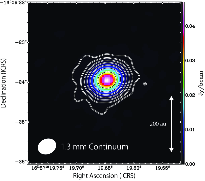
Figure 1: Images of the 1.3 mm dust continuum. The peak position is ($\alpha_{IRCS}$, $\delta_{IRCS}$) = (16^h57^m19$\fs$647, $-$16°9′23$\farcs$94). The rms noise level ($\sigma$) is 40 $\mu$Jy beam^-1. The contours levels start at $10\sigma$ and double in value up to $640\sigma$. A white ellipse represents the beam size.

Figure 1 shows the 1.3 mm continuum map whose beam size is 0$\farcs$47 $\times$ 0$\farcs$39 (P.A.: $-$65$.\!\!$°2). This has a higher angular resolution than the 1.2 mm continuum map, and hence, we here use the 1.3 mm data in the present study. The continuum emission is concentrated around the protostar. The peak position determined by a 2D Gaussian fit is ($\alpha_{\rm IRCS}$, $\delta_{\rm IRCS}$) = (16^h57^m19$\fs$647, $-$16°09′23$\farcs$94). The integrated flux density and peak flux density are $55.9\pm 1.1$ mJy and $47.1\pm 0.6$ mJy beam^-1, respectively. The peak intensity corresponds to a brightness temperature of $5.73\pm 0.07$ K. The source image size is (0$\farcs$473 $\pm$ 0$\farcs$006) $\times$ (0$\farcs$459 $\pm$ 0$\farcs$005) with P.A. of 123^∘ $\pm$ 16^∘. This corresponds the linear size of $(66.2\pm 0.8)$ au $\times(64.2\pm 0.8)$ au. Since the image size is comparable to the beam size, the deconvolution is not successful. The source is very compact. Detailed analyses of the dust emission will be described in a separate publication of FAUST.

3.2 Molecular Distributions

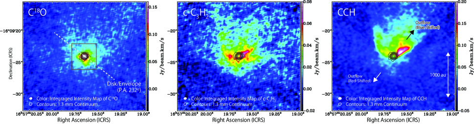
Figure 2: Integrated intensity maps (moment 0 maps) of C¹⁸O ($J=2-1$), c-C₃H₂ ($6_{0,6}-5_{1,5}$; $6_{1,6}-5_{0,5}$), CCH ($N=3-2,J=7/2-5/2$) (Color) and the continuum image (black contours; Figure 1). The integrated velocity range is from 0.0 km s^-1 to 9.8 km s^-1 for the three lines, where the systemic velocity is 5.0 km s^-1. A dashed line on the left panel indicates the direction of the disk/envelope system which is perpendicular to the CO outflow direction (P.A. 142^∘) (Wu et al., 1996; Vallée et al., 2000). The rms noise level is 7 mJy beam^-1 km s^-1 for the three maps. A dashed rectangle in the C¹⁸O panel indicates the area for Figures 1, 5, 9, and 10. The beam sizes are shown on a bottom left corner of each panel.

Figure 2a shows the integrated intensity map of the C¹⁸O ($J=2-1$) line. The distribution of C¹⁸O traces the protostellar core on a scale of 4″ (560 au) around the protostar with its intensity peak coinciding the continuum position. Figures 2b and 2c show the integrated intensity maps of the unsaturated hydrocarbon molecule lines, c-C₃H₂ ($6_{0,6}-5_{1,5}$, $6_{1,6}-5_{0,5}$) and CCH ($N=3-2$, $J=7/2-5/2$), respectively. The overall extent of the c-C₃H₂ emission is comparable to that of C¹⁸O, indicating that c-C₃H₂ exists in the protostellar core traced by C¹⁸O. Nevertheless, the distributions are different between c-C₃H₂ and C¹⁸O. The c-C₃H₂ emission does not peak at the continuum peak position but shows a rather extended structure to the northwestern and eastern directions. Moreover, the weak emission seems to extend more to the northern part than to the southern part. These features can be seen more clearly in the CCH emission map. The molecular outflow is aligned along the northwest-southeast direction, and hence, the CCH emission seems to be enhanced in the outflow cavity wall, as seen in IRAS 15398-3359 and NGC1333 IRAS4C (Oya et al., 2014; Zhang et al., 2018; Oya et al., 2018b). Therefore, the northwestern feature of c-C₃H₂ may also be affected by the outflow.

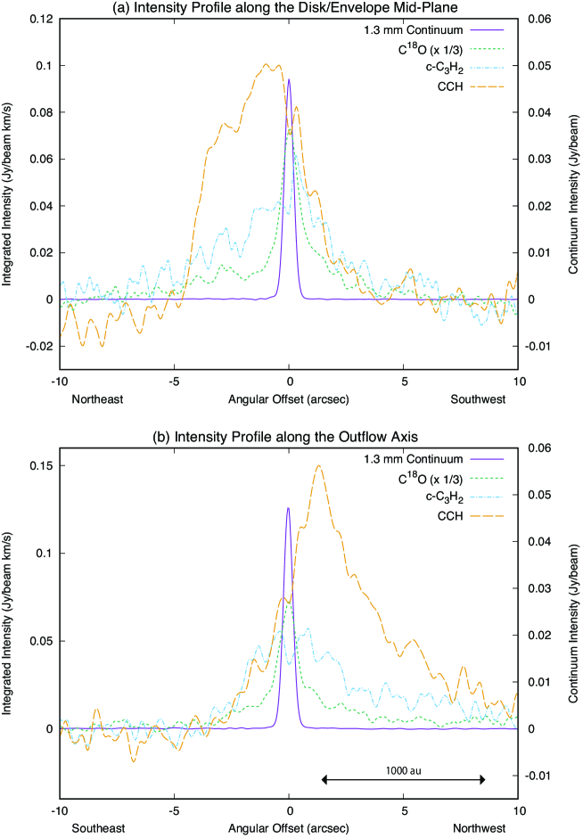
Figure 3: (a) Intensity profiles of the C¹⁸O ($J=2-1$), c-C₃H₂ ($6_{0,6}-5_{1,5}$; $6_{1,6}-5_{0,5}$), CCH ($N=3-2,J=7/2-5/2$), and the 1.3 mm dust continuum emission along the disk/envelope direction (P.A.232^∘) indicated in the left panel of Figure 2 and (b) those along the outflow axis (P.A. 142°). The position is the offset from the continuum peak position. The rms noise level is 7 mJy beam^-1 km s^-1 for the C¹⁸O, c-C₃H₂, and CCH lines, while it is 40 $\mu$Jy beam^-1 for the continuum emission.

Figure 3a shows the intensity profiles of the C¹⁸O, c-C₃H₂, CCH, and continuum emission along a line passing through the continuum peak with a P.A. of 232^∘. This direction is perpendicular to the position angle of the previously reported outflow (Wu et al., 1996; Vallée et al., 2000), and hence, Figure 3a reveals the intensity profile along the disk/envelope system. The intensities of c-C₃H₂ and CCH tend to increase approaching the protostar, although that of CCH seems heavily affected by the outflow. Association of c-C₃H₂ and CCH with the protostar on a 1000 au scale indicates that CB68 is characterized by WCCC (e.g., Sakai et al. 2008; Aikawa et al. 2008; Sakai & Yamamoto 2013). For a reference, the intensity profiles along the outflow direction are shown in Figure 3b. Although the distribution of c-C₃H₂ is centrally concentrated, the CCH emission shows an extension to the northwestern side along the outflow. Such extension is seen in the integrated intensity map of Figure 2c.

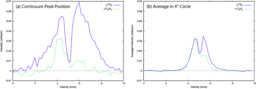
Figure 4: (a) Observed spectra of C¹⁸O ($J=2-1$) and c-C₃H₂ ($6_{0,6}-5_{1,5}$; $6_{1,6}-5_{0,5}$) at the continuum position. (b) Observed spectra of C¹⁸O and c-C₃H₂ averaged over the circular area of 4$\farcs$0 in diameter around the continuum peak.

The fractional abundance of c-C₃H₂ relative to H₂ at the continuum peak position is derived in the following way. Here, we use the C¹⁸O emission to derive the H₂ column density. Figure 4a shows the spectra of c-C₃H₂ and C¹⁸O at the continuum position. The spectrum of c-C₃H₂ shows self-absorption of the red-shifted component due to an infalling motion and that of the systemic velocity component due to the foreground gas (e.g., Evans et al. 2015; Yang et al. 2020). To minimize these effects, we conservatively employ the blue-shifted component, which is less affected by these effects, in the fractional abundance derivation. The peak intensities of the blue-shifted emission measured by the Gaussian fit are 32 mJy beam^-1 and 54 mJy beam^-1 for c-C₃H₂ and C¹⁸O, respectively. From these values, the column densities of the blue-shifted component of c-C₃H₂ and C¹⁸O are derived to be ($2.4-3.5)\times 10^{13}$ cm^-2 and $5.4\times 10^{15}$ cm^-2, respectively, by using the non-LTE (local thermodynamic equilibrium) radiative transfer code, RADEX. For this calculation the linewidths of 1.05 km s^-1 are used for the both species, and the H₂ volume densities of $10^{6}-10^{8}$ cm^-3 are assumed. This is a range of the H₂ density of a typical protostellar envelope (Sakai et al., 2014b). The gas kinetic temperature is uncertain. We adopt 25 K for it, which is the desorption temperature of CH₄ for triggering WCCC (Sakai et al., 2008; Sakai & Yamamoto, 2013). The column density for each species is derived to match the intensity calculated by RADEX with the observed one. The maximum optical depths of the c-C₃H₂ and C¹⁸O lines are 0.55 and 0.42, respectively. Then, the fractional abundance of c-C₃H₂ relative to H₂ is roughly estimated to be $(0.7-1.0)\times 10^{-9}$, where the H₂ column density is evaluated from the C¹⁸O column density to be $\sim 3.6\times 10^{22}$ cm^-2 by using the empirical equation for the high C¹⁸O column density case ($>3\times 10^{14}$ cm^-2) reported by Frerking et al. (1982). If we assume the gas kinetic temperatures of 15 K and 35 K, the fractional abundances of c-C₃H₂ are $(0.8-2.1)\times 10^{-9}$ and $0.6\times 10^{-9}$, respectively. In this case, the maximum optical depths of c-C₃H₂ and C¹⁸O are 1.5 and 1.1, respectively, for the H₂ density of $10^{6}$ cm^-3 and the temperature of 15 K. Hence, the estimated range of the fractional abundance of c-C₃H₂ is $(0.6-2.1)\times 10^{-9}$ in CB68, which is lower by one or two orders of magnitude than the value found for L1527 ($2.7\times 10^{-8}$) (Sakai et al., 2010).

The low abundance may originate from the above analysis focused on the protostellar position with a narrow beam ($\sim 70$ au). Then, we also calculate the fractional abundance range of c-C₃H₂ averaged over the circular area of 4$\farcs$0 (560 au) in diameter centered at the protostar position, which is comparable to the distribution of c-C₃H₂. Figure 4b shows the spectra of c-C₃H₂ and C¹⁸O averaged over the area. The self-absorption feature of the red-shifted component and the systemic velocity component is also seen as in the above case, and hence, we employ the blue-shifted component for the fractional abundance evaluation. Through the procedure mentioned above, we obtain the range of the fractional abundance of c-C₃H₂ of $(0.9-4.2)\times 10^{-9}$, which is not much different from that derived with the narrow beam. In this case, the maximum optical depths of c-C₃H₂ and C¹⁸O are 1.6 and 0.5, respectively, for the H₂ density of $10^{6}$ cm^-3 and the temperature of 15 K. These analyses imply that the enhancement of the c-C₃H₂ abundance due to the WCCC effect is weaker in CB68 than in L1527.

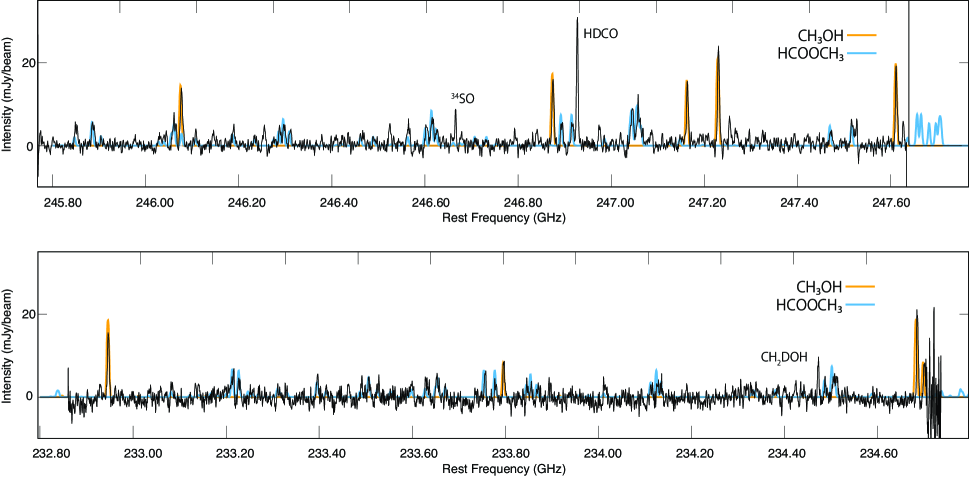
Figure 6: Observed spectra of the two continuum bands for demonstration of rich iCOM lines (black lines). The systemic velocity of 5.0 km s^-1 is adopted to calculate the rest frequency. Colored ones are the results of the simulation based on the column density, the rotation temperature, and the beam filling factor derived in the analysis. See Section 3.3 for details. Orange lines represent CH₃OH, whereas blue ones HCOOCH₃.

On the other hand, CH₃OH is concentrated around the protostar on a scale of 100 au or smaller, as shown in Figures 5a and 5b, where the low-excitation line ($4_{2,3}-3_{1,2}$ E; $E_{\mathrm{u}}/k_{\mathrm{B}}=45.46$ K) and the high-excitation line ($16_{2,15}-15_{3,13}$ E; $E_{\mathrm{u}}/k_{\mathrm{B}}=338.14$ K) are depicted, respectively. Here, $k_{\mathrm{B}}$ stands for the Boltzmann constant. The CH₃OH lines show a compact distribution and are not resolved by the synthesized beam. In total, 11 lines of CH₃OH are detected (Table 1). In addition, CH₂DOH, HCOOCH₃ and CH₃OCH₃ are detected, as listed in Table 1. Here, the detection criterion is that the integrated intensity is higher than the $3\sigma$ noise level. To identify these molecules, we visually inspect all the lines of a certain species in the observed spectral windows, confirming that line intensities are self-consistent. For HCOOCH₃, there are several faint lines in the continuum bands (Figure 6), which are reasonably explained by the calculated spectrum using the column density and the rotation temperature derived below. Similarly, all the intensities of the identified lines are consistent, from a posteriori check, with the derived column densities and rotation temperatures. Examples of the moment 0 maps of HCOOCH₃ and CH₃OCH₃ are shown in Figures 5c and 5d, respectively. Their distributions are compact around the protostar and are not resolved by the synthesized beam ($\sim$ 0$\farcs$4$-$0$\farcs$5; $\sim$70$-$80 au), as in the case of the high-excitation line of CH₃OH.

We carefully check the other iCOM lines by using their simulated spectra, as applied to the HCOOCH₃ lines in the above paragraph. We notice that a line at 234471 MHz could match with the $3_{3,1}-3_{2,2}$ E line of CH₃CHO (234469 MHz). However, this line is overlapped with the CH₂DOH line ($8_{2,6}-8_{1,7}$ e₀; 234471 MHz), and moreover, the other CH₃CHO lines nearby this line, which are expected to be of equivalent intensity or brighter, are not detected. We thus conclude that CH₃CHO is not detected in these observations. Following a similar procedure, we also conclude that NH₂CHO, C₂H₅OH, HCOOH, CH₃COCH₃, and C₂H₅CN are non-detection (Table 1).

In CB68, the carbon-chain related species (unsaturated hydrocarbon), c-C₃H₂, is concentrated around the protostar on a scale of 1000 au, a signature of WCCC. In contrast, compact distributions of iCOMs are also found on a scale of 100 au or smaller, which is evidence for hot corino chemistry. Hence, CB68 can be regarded to have a hybrid chemistry, where WCCC and hot corino chemistries coexist but on different scales. Such chemical characteristics have been found in other low-mass protostellar sources such as L483 and B335 (Imai et al., 2016; Oya et al., 2017). It is important to emphasize that the above chemical structure found in CB68 is similar to that found in B335, which is also an isolated protostellar source. For quantitative comparison with the other sources in Section 3.4, we derive the molecular column densities in the following sub-section.

3.3 Abundances of iCOMs

First, the column density ($N$) and the rotation temperature ($T_{\rm rot}$) of CH₃OH at the continuum peak are derived under the assumption of LTE. The emitting region for the high-excitation lines of CH₃OH is very compact around the protostar, where the density is high enough for the LTE approximation to hold. We use the following equation that considers the effect of optical depth on the observed intensity (Yamamoto, 2017):

$$T_{\mathrm{obs}}=f\ \left(\frac{c^{2}}{2k_{\mathrm{B}}\nu^{2}}\right)(B_{\nu}(T_{\mathrm{rot}})-B_{\nu}(T_{\mathrm{b}}))(1-\exp(-\tau)),$$ (1)

and

$$\tau=\frac{8\pi^{3}S\mu^{2}}{3h\Delta vU(T)}\left[\exp\left(\frac{h\nu}{k_{\mathrm{B}}T}\right)-1\right]\exp\left(\frac{-E_{\mathrm{u}}}{k_{\mathrm{B}}T}\right)N,$$ (2)

where $B_{\nu}(T)$ denotes the Planck function, $U(T)$ the partition function of the molecules at the excitation temperature $T$, $N$ the column density, $\nu$ the frequency of the line, $E_{\mathrm{u}}$ the upper state energy, $f$ the beam filling factor, and $T_{\mathrm{b}}$ the cosmic microwave background temperature (2.7 K).

The CH₃OH lines used in the least-squares analysis are listed in Table 1. Among them, we find that the optical depths for the two low-excitation lines ($4_{2,3}-3_{1,2}$ E, 218440 MHz, $E_{\mathrm{u}}/k_{\mathrm{B}}$ = 45.46 K; $5_{1,4}-4_{1,3}$ A, 243916 MHz, $E_{\mathrm{u}}/k_{\mathrm{B}}$ = 49.66 K) are higher than 6. Conservatively, to minimize opacity effects, we use the lines for which the opacity is less than 2. The rotation temperature, the column density, and the beam-filling factor are determined by the least-squares analysis on the peak intensities which are derived by dividing the integrated intensity by the line width (6 km s^-1). The largest correlation coefficient between the parameters in the least-squares fit is 0.68 between the column density and the beam filling factor. Hence, the parameters are well determined in the fit. The rotation temperature and the column density are derived to be $131\pm 11$ K and $(2.7\pm 1.0)\times 10^{18}$ cm^-2, respectively, where the errors represent the standard deviation of the fit. The beam filling factor is well constrained and determined to be $0.022\pm 0.003$. Since the high-excitation lines used in the analysis are not spatially resolved with the current synthesized beam, the small beam-filling factor is reasonable. This means that the CH₃OH emission, particularly for the high-excitation lines, mainly comes from a very compact region whose size is approximately 10 au. The maximum optical depth among the fitted lines is 1.9 for the $4_{2,2}-5_{1,5}$ A line. In Figure 6, the calculated spectrum of CH₃OH is overlaid on the two spectral windows. The observations are well-reproduced by the spectrum calculated by using the best-fit parameters.

Similarly, the column density of HCOOCH₃ is derived using the least-squares fit on the observed lines listed in Table 1, where Equation (1) is employed. Here, heavily blended lines are excluded in the analysis. Although we have tried to determine the column density, the rotation temperature, and the beam-filling factor simultaneously, the rotation temperature and the beam-filling factor are not well determined in the fit. This is due to a relatively poor signal-to-noise ratio of the spectra. Hence, we determine the column density of HCOOCH₃ by assuming the rotation temperature and the beam-filling factor measured for CH₃OH. This assumption is justified, because the emitting region of the high-excitation lines of CH₃OH and that of the HCOOCH₃ lines are likely to be similar (i.e., a hot corino). Nevertheless, we also evaluate the column density by assuming the rotation temperature of 100 K and 150 K, in order to investigate the dependence of the column density on the assumed temperature. The results are shown in Table 2. The HCOOCH₃ spectrum calculated for the 131 K case is overlaid on Figure 6, which is consistent with the observation.

The column densities of CH₃OCH₃ and CH₂DOH are derived in a similar way as HCOOCH₃ discussed above (Table 2). Specifically, the rotation temperature and the beam-filling factor are fixed to the values derived from CH₃OH because of small numbers of detected lines. The column densities are also evaluated assuming the rotation temperature of 100 K and 150 K. Note that the CH₂DOH ($4_{1,4}-4_{1,3}$ $e_{1}-e_{0}$) line at 246973 MHz was not included in the fit, because the line strength of this inter-vibrational transition is uncertain (Pickett et al., 1998). Recently, the uncertainty of the line strength for this molecule has also been pointed out by Ambrose et al. (2021).

We derive the $3\sigma$ upper limits to the column densities of NH₂CHO, CH₃CHO, C₂H₅OH, HCOOH, CH₃COCH₃, and C₂H₅CN, assuming the rotation temperature and the beam filling factor derived in the CH₃OH analysis. They are also evaluated assuming a rotation temperature of 100 K and 150 K. For this purpose, we simulate the spectrum of each molecule in all the spectral windows of our observations and select the highest intensity line for derivation of the upper limit. The upper limit to the column density is then evaluated from the $3\sigma$ upper limit to the integrated intensity. The line width is assumed to be 6 km s^-1. This is the average line width of the detected iCOMs in this observation. The derived upper limits are summarized in Table 2.

3.4 Comparison with Other Sources

In this section, we compare the molecular abundances of iCOMs in CB68 to those in several hot corinos observed with interferometers. To this end, column density ratios in between iCOMs are used instead of the fractional abundance relative to H₂, because the H₂ column density for the emitting region of iCOMs is not available in this source. The HCOOCH₃/CH₃OH ratio in CB68 is derived to be $0.09^{+0.07}_{-0.03}$. This ratio is slightly higher than values found in the other sources harboring a hot corino: IRAS 16293$-$2422 Source A ($0.021^{+0.011}_{-0.008}$; Manigand et al., 2020), IRAS 16293$-$2422 Source B ($0.026^{+0.008}_{-0.007}$; Jørgensen et al., 2018), NGC1333 IRAS2A ($0.016^{+0.012}_{-0.007}$; Taquet et al., 2015), B1-c ($0.010^{+0.005}_{-0.002}$; van Gelder et al., 2020), Ser-emb 8 ($0.011^{+0.009}_{-0.004}$; van Gelder et al., 2020), and L1551 IRS5 ($0.033\pm 0.002$; Bianchi et al., 2020). The CH₂DOH/CH₃OH ratio is derived to be $0.06^{+0.04}_{-0.02}$. This is close to the corresponding ratios in other hot corinos: IRAS 16293$-$2422 Source A ($0.09^{+0.04}_{-0.03}$; Manigand et al., 2020), IRAS 16293$-$2422 Source B ($0.07\pm 0.02$; Jørgensen et al., 2018), B1-c ($0.08^{+0.04}_{-0.02}$; van Gelder et al., 2020), and Ser-emb 8 ($0.043^{+0.033}_{-0.014}$; van Gelder et al., 2020). It should be noted that the intrinsic line strength of CH₂DOH could be uncertain (Ambrose et al., 2021), so that the derived ratio may be changed by a factor of a few.

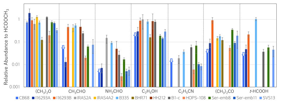
Figure 7: Comparison of relative abundances to HCOOCH₃ with several low-mass protostellar souces. Source names are given on the right hand side. I16393A denotes IRAS16293$-$2422 Source A, I16393B denotes IRAS16293$-$2422 Source B, IRAS2A denotes NGC1333 IRAS2A, IRAS4A2 denotes NGC1333 IRAS4A2, and BHR71 denotes BHR71 IRS1. See Table 3 for references.

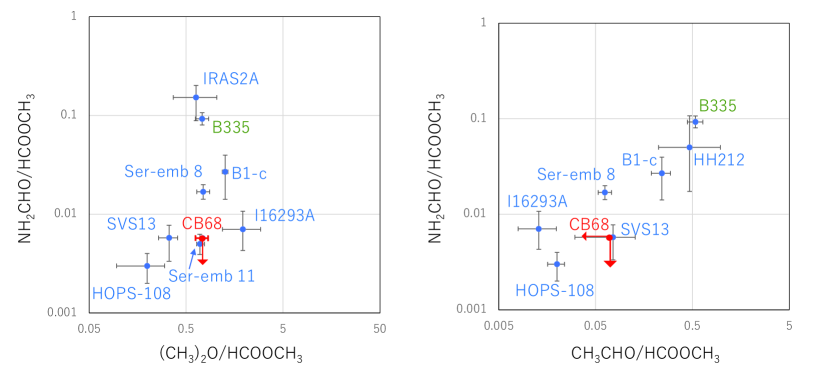
Figure 8: (left) Plot of the abundances of CH₃OCH₃ and NH₂CHO relative to HCOOCH₃. (right) Plot of the abundances of CH₃OCH₃ and NH₂CHO relative to HCOOCH₃.

Since the CH₃OH abundance when considering the effect of optical depth is not always available for several hot corinos and would have a large uncertainty, the ratio relative to HCOOCH₃, which is likely optically thin in all the sources, is used for comparison to other iCOMs, as summarized in Table 3 and Figure 7. The CH₃OCH₃/HCOOCH₃ and C₂H₅OH/HCOOCH₃ ratios do not vary among the sources very much. Indeed, the CH₃OCH₃/HCOOCH₃ ratio in CB68 is $0.74\pm 0.11$, which is almost comparable to those for the other sources. A trend of the constant CH₃OCH₃/HCOOCH₃ ratio is also reported by (Chahine et al., 2022). On the other hand, the other ratios shows some variation from source to source. Although only $3\sigma$ upper limits to the ratio relative to HCOOCH₃ are obtained for the other species, the CH₃CHO/HCOOCH₃, NH₂CHO/HCOOCH₃, and HCOOH/HCOOCH₃ ratios in CB68 tend to be low among the other hot corinos. Hence, CH₃CHO, NH₂CHO, and HCOOH seem relatively less abundant in CB68. Such a trend for CH₃CHO and NH₂CHO can also be seen in Figure 8. In particular, the difference is significant between the two isolated sources, CB68 and B335. Meanwhile, the upper limits to the C₂H₅OH/HCOOCH₃, C₂H₅CN/HCOOCH₃, and CH₃COCH₃/HCOOCH₃ ratios are comparable to the corresponding ratios in the other sources. Table 3 lists the bolometric luminosity and the bolometric temperature of each source. The deficiency of CH₃CHO, NH₂CHO, and HCOOH in CB68 is not simply ascribed to these physical parameters.

It should be noted that the dust continuum emission can be optically thick at millimeter wavelengths. Although the beam-averaged brightness temperature of the dust emission in CB68 is $5.73\pm 0.07$ K, the dust opacity could be higher for the emitting region of CH₃OH. A detailed analysis of the dust emission is left for future study that includes analysis of the other ALMA frequency bands. Here, we just discuss the effect of optically thick dust on the observed molecular abundances. If the emitting region is the same for all the iCOMs observed in this study, the optically thick dust would not seriously affect the above discussions on the abundance ratios. The effect is compensated at least partially by taking the column density ratios. However, the distribution of the emission could be different from iCOM to iCOM. For instance, N-bearing iCOMs such as NH₂CHO and C₂H₅CN would be more centrally concentrated around the protostar than O-bearing iCOMs such as HCOOCH₃ and CH₃OCH₃, as revealed in the high-mass protostellar sources (e.g., Jiménez-Serra et al. 2012; Feng et al. 2015; Csengeri et al. 2019). Such a trend has recently been found in the low-mass protostellar source L483 (Oya et al., 2017; Okoda et al., 2021b). If this were also the case of CB68, N-bearing iCOMs would be more affected by the optically thick dust. In this case, the apparent abundances of N-bearing iCOMs relative to HCOOCH₃ would be lower. Even if the dust opacity is not high, the smaller distribution yields a lower beam-averaged column density for the same beam filling factor. According to Csengeri et al. (2019), HCOOH shows a distribution like N-bearing iCOMs. Hence, the low abundance of HCOOH relative to HCOOCH₃ would also be attributed to its very compact distribution. In the following discussions, we need to keep these caveats in mind.

3.5 Comparison with Chemical Models

Here, we compare the observed molecular abundances with the reported results of chemical network calculations. We first employ the detailed chemical model of hot cores/hot corinos with an emphasis on iCOMs reported by Garrod et al. (2022) for comparison (Table 4). This model is an updated version of that reported by Garrod (2013). In those works, a three-phase model is used, where chemical processes in the gas-phase, on grain-surface, and in bulk-ice are fully incorporated. Temporal variations of molecular abundances are calculated for the three different warm-up processes, which mimic protostellar birth: namely, fast, medium, and slow warm-up processes from the cold cloud stage (10 K) to the hot corino stage (100 K). In the model by Garrod et al. (2022), the HCOOCH₃/CH₃OH ratio is 0.02 for the fast warm-up case and becomes slightly higher for slower warm-up cases. The model result is roughly consistent with the range of the ratio observed for the hot corino sources including CB68. The CH₃OCH₃/HCOOCH₃ ratio calculated by the model is 0.6-0.9 and does not vary significantly among the three warm-up cases. In the hot corino sources, the ratio is 0.12$-$1.9, and hence, the model result fits the observations. The CH₃CHO/HCOOCH₃ ratio is 0.21 for the fast warm-up case and slightly increases for slower warm-up cases. It is much larger than the upper limit derived in CB68, while it is consistent with some hot corinos as shown in Table 3 and Figure 7. The abundance of NH₂CHO calculated in the fast warm-up model is 1/10 of that of HCOOCH₃, which is inconsistent with the upper limit measured for CB68 ($<0.006$). Note that the calculated NH₂CHO/HCOOCH₃ ratio becomes slightly higher for a slower warm-up period in the model. It is still higher than the observed ratio for the most of sources except for NGC1333 IRAS2A.

On the other hand, Aikawa et al. (2020) presented chemical network calculations considering the physical evolutions of the static and collapsing phases, where the physical condition is taken from the 1D radiation hydrodynamic model of low-mass star formation presented in Masunaga et al. (1998) and Masunaga & Inutsuka (2000). Their results successfully reproduce both of the chemical features observed in CB68: (1) the enhancement of carbon-chain molecules and related species on a 1000 au scale (i.e., WCCC) and (2) enrichment of iCOMs in the vicinity of the protostar (i.e., hot corino chemistry). The chemical network is essentially the same as that reported by Garrod (2013) except for some updates of the reactions. However, the detailes of the ice chemistry model, i.e., multi-layered ice mantle without swapping, are different from Garrod (2013), which affect the iCOM abundances.

According to Aikawa et al. (2020), the HCOOCH₃/CH₃OH and CH₃OCH₃/HCOOCH₃ abundance ratios in the hot corino stage derived from the chemical network calculation is much lower and higher, respectively, than the observational results for the hot corino sources including CB68. Aikawa et al. (2020) also reported that the CH₃OCH₃/HCOOCH₃ ratio depends on the lowest temperature $T_{\rm{min}}$ during the evolution. The ratio changes by two orders of magnitude, where it is close to unity for the case of $T_{\rm{min}}$ of 20 K: the ratio is higher for the lower and higher $T_{\rm{min}}$ in the range from 10 K to 25 K. For $T_{\rm{min}}$ of 20 K, the CH₃OCH₃/HCOOCH₃ ratio is almost comparable to the observed ratios in hot corinos, while the CH₃CHO/HCOOCH₃ and NH₂CHO ratios are much overestimated. The HCOOCH₃ abundance seems much underestimated, and resolving this issue is left for a future study.

4 Kinematic Structure

In this section, we explore the kinematic structure of the hot corino and its surrounding envelope. We assume the P.A. of the disk/envelope system to be 232°, perpendicular to the outflow direction (P.A. = 142°) (Wu et al., 1996; Vallée et al., 2000; Launhardt et al., 2010). The disk/envelope direction is shown by dashed lines of Figure 2a.

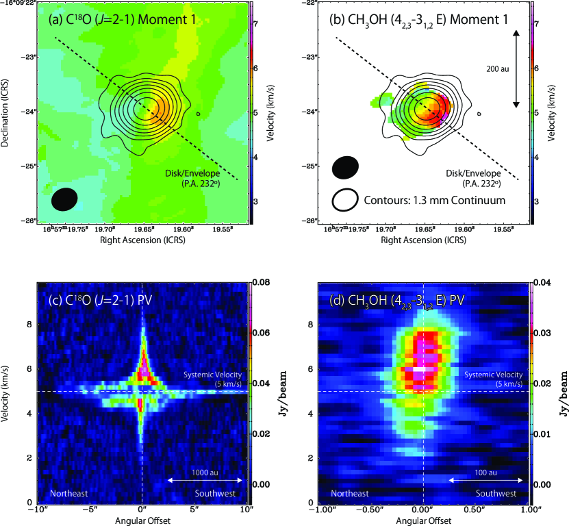
Figure 9: (a, b) The velocity field maps (moment 1 maps) of C¹⁸O and CH₃OH. Black closed ellipses represent the beam sizes. The cube data with the intensity less than 3$\sigma$ are not used. Furthermore, the positions with the integrated intensity less than 3$\sigma$ are shown in white. Contours represent the continuum image of Figure 1, where a black open ellipse shows its beam size. Dashed lines represent the disk/envelope direction, along which the position velocity diagrams are presented. (c) The position velocity diagram of C¹⁸O along the disk/envelope direction shown in Figure 2. (d) The position velocity diagram of CH₃OH along the disk/envelope direction. A smaller range of the position offset is employed to see the velocity gradient clearly.

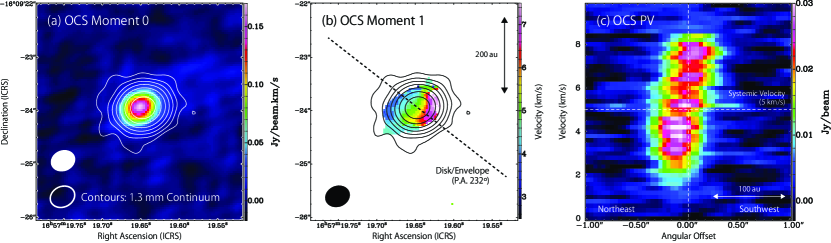
Figure 10: The integrated intensity map (left), the moment 1 map (middle), and the PV diagram of OCS along the disk/envelope direction (right), where a dashed line in the middle panel shows the disk/envelope direction, The velocity range for the integrated intensity map is from 0.0 km s^-1 to 9.8 km s^-1. Contours on the left and middle panels represent the continuum emission (Figure 1). See the caption of Figure 9 for preparation of the moment 1 map. The rms noise level of the integrated intensity map is 4 mJy beam^-1 km s^-1. On the left panel, a white closed ellipse represents the beam size of the OCS image, while a white open ellipse that of the 1.3 mm continuum image. On the middle panel, a black closed ellipse represents the beam size of the OCS image. A velocity gradient is visible in the moment 1 map and the PV map.

Figures 9a and 9b show the moment 1 maps of the C¹⁸O ($J=2-1$) line and the low-excitation line ($4_{2,3}-3_{1,2}$ E) of CH₃OH. A velocity gradient along the disk/envelope direction is seen for these two lines, although the gradient in the moment 1 map of C¹⁸O looks marginal due to the contribution of the extended component. To investigate the velocity structure in more detail, we draw position-velocity (PV) diagrams along the disk/envelope direction. Figure 9c shows the PV diagram of the C¹⁸O line along the disk/envelope direction. A diamond shape feature can be seen, where the velocity width increases approaching the protostar. Moreover, a marginal velocity gradient, suggesting a rotation motion, is found in the vicinity of the protostar: the southwestern side is red-shifted, while the northeastern side is blue-shifted. This velocity gradient is more clearly seen in the PV diagram of the low-excitation CH₃OH line observed with the high frequency-resolution spectral window (Figure 9d). Although the blue-shifted emission is rather faint, the velocity gradient is consistent with that found in C¹⁸O. For further confirmation, we investigate the velocity structure of the OCS ($J=19-18$) emission, which is concentrated around the protostar (Figure 10a). Figure 10b shows the moment 1 map, while Figure 10c depicts the PV diagram along the disk/envelope direction. OCS is also reported to be enhanced in the inner envelope of IRAS 16293$-$2422 Source A as well as iCOMs (Oya et al., 2016). The velocity gradient ($\sim 0.07$ km s^-1 au^-1) is clearly seen in the moment 1 map and the PV diagram of OCS.

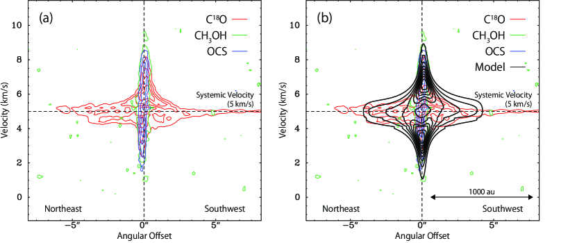
Figure 11: (a) A composite PV diagram of C¹⁸O (red), CH₃OH (green), and OCS (blue), which represents the kinematic structure for a wide spatial range. (b) Same as (a) with the result of the infalling rotating envelope model using the fiducial values of the model parameters (black contours). See Section 4 for details. The position shows the offset from the continuum peak.

The diamond shape structure seen in the PV diagram of C¹⁸O is a typical feature characteristic of an infalling-rotating envelope (IRE), where the gas is infalling with conserved angular momentum (Ohashi et al., 1997; Sakai et al., 2014a; Oya et al., 2014, 2016). The PV diagram further shows a counter velocity component (blue-shifted emission in the southwestern part and red-shifted emission in the northeastern part). Such feature is difficult to explain by a Keplerian motion alone. To compare the kinematic structures of the above molecules, we present a composite PV diagram, where the individual PV diagrams of the C¹⁸O, CH₃OH, and OCS lines are overlaid in the same panel (Figure 11a). Although the distribution of the CH₃OH line is not well resolved, its kinematic structure resembles that of the OCS line. While C¹⁸O seems to trace an entire IRE, CH₃OH and OCS most likely trace its innermost part.

Although the velocity gradient is small, we try to roughly estimate physical parameters of the IRE. For this purpose, we compare the kinematic structures observed for the C¹⁸O, CH₃OH, and OCS lines with that derived from a simple model of IREs. Details of the model are described in Oya et al. (2014). This model has successfully been applied to the IREs of some low-mass protostellar sources (e.g., Sakai et al. 2014a; Oya et al. 2015; Oya et al. 2016; Oya et al. 2017; Imai et al. 2019; Oya & Yamamoto 2020). In this model, the structure of the IRE is determined by six free parameters: the kinematic structure is specified by (1) the radius of the centrifugal barrier ($r_{\mathrm{CB}}$) and (2) the mass of the central protostar ($M_{\ast}$), while the shape of the IRE is specified by (3) the outer radius of the emitting region in the envelope ($R_{\mathrm{0}}$), (4) the full thickness of the envelope ($h_{\mathrm{0}}$), (5) the flare angle of the envelope, and (6) the inclination angle ($i$) with respect to the line of sight ($i=90^{\circ}$ for the edge-on case).

In the CB68 model, we make the following assumptions. The outer radius is fixed to be 600 au by referring the distribution of the C¹⁸O emission. We assume the inclination angle to be 70° (nearly edge-on disk). This assumption seems reasonable because the well-collimated outflow feature (Vallée et al., 2000) suggests the nearly edge-on geometry of the disk. Moreover, the fitting results do not depend on inclination angles ranging from 50° to 90°, although the protostellar mass is correlated with it ($\propto sin^{-2}i$). We arbitrarily assume a flare angle of the envelope of 10° and that the full thickness of the envelope is 100 au. We confirm that the results do not significantly change for a flare angle between 0° and 30° and for a thickness between 10 au to 100 au. This is because the resolution of the present observation ($\sim$0$\farcs$4$-$0$\farcs$5; 70$-$80 au) is insufficient to place strong constraints on these parameters.

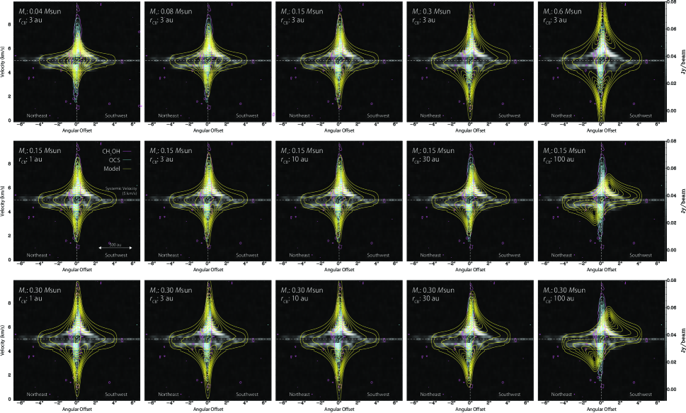
Figure 12: Results of the infalling rotating envelope model with various parameters (yellow contours) superposed on the composite PV diagram shown in Figure 11a. C¹⁸O is presented in gray scales, CH₃OH in magenta, and OCS in cyan. The position shows the offset from the continuum peak. The protostellar mass of 0.08$-$0.30 $M_{\odot}$ and the radius of the centrifugal barrier ($r_{\rm CB}$) of 30 au or smaller can reasonably reproduce the observed kinematic structure.

Figure 11b shows the result of the model calculation overlaid on the composite PV diagram. The velocity structure including the counter velocity component seems to be reproduced with $r_{\mathrm{CB}}$ of 3 au and $M_{\ast}$ of 0.15 $M_{\odot}$. We use these values as the fiducial values to find the acceptable ranges of the parameters. To estimate the ranges of $r_{\mathrm{CB}}$ and $M_{\ast}$, we change their values from the above fiducial ones and compare the results with the composite PV diagram by eye. Figure 12 shows a comparison with the composite PV diagram. In the comparison, we focus on the overall velocity extent rather than the detailed intensity distribution because the latter is difficult to be reproduced quantitatively due to various factors such as the self-absorption effect and inhomogeneous distribution not considered in the IRE model. The velocity shift is mainly affected by $M_{\ast}$ because the velocity of the gas at a certain radius is roughly proportional to $M_{\ast}^{1/2}$ in the IRE model. Considering that the OCS and CH₃OH emission has higher velocity component than the C¹⁸O emission around the protostar position, we conservatively adopt the ranges from 0.08 $M_{\odot}$ to 0.30 $M_{\odot}$ for $M_{\ast}$. On the other hand, $r_{\mathrm{CB}}$ affects the velocity gradient in the PV diagram. The observed PV diagrams can be reasonably explained by $r_{\mathrm{CB}}$ less than 30 au for the models assuming $M_{\ast}$ of 0.15 $M_{\odot}$. This result is not changed if $M_{\ast}$ is changed in the above range. For instance, the case for 0.3 $M_{\odot}$ is shown in Figure 12 (bottom panel).

5 Comparison with B335

In this section, we discuss the similarities and differences between CB68 and B335, both of which are isolated Class 0 protostellar sources in Bok globules and have similar bolometric luminosity and bolometric temperature (Table 3). Note that BHR71 IRS1 is also a Class 0 protostar in a Bok globule, whose chemical compositions may be compared with those of CB68 in the context of the isolated protostars. However, this source accompanies another protostar IRS2 separated from IRS1 by 16″, and hence, it is not in a fully isolated condition like CB68 and B335. Furthermore, the abundances are obtained for a limited species, and the data of NH₂CHO and CH₃CHO, which show relatively low abundances in CB68 are not available (Yang et al., 2020). For these reasons, we do not particularly discuss BHR71 IRS1 for detailed comparison with CB68 in this paper.

The protostellar mass of CB68 estimated in this study is likely higher than the mass of B335 (0.02$-$0.06 $M_{\odot}$; Imai et al., 2019). Only the upper limit to the radius of the centrifugal barrier is obtained for the both sources ($<$ 5 au for B335 and $<$ 30 au for CB68). These radii are smaller than those previously reported for the other protostellar sources L1527 ($100\pm 20$ au: Sakai et al., 2014b), IRAS 16293$-$2422 Source A (40$-$60 au: Oya et al., 2016), and TMC-1A ($\sim 50$ au: Sakai et al., 2016). The comparatively small centrifugal barrier indicates a relatively small specific angular momentum of the accreting gas and that the infalling motion is dominant in the protostellar envelope. Hence, the Keplerian disk has not grown to a sufficient size to be detected inside the centrifugal barrier. Although we cannot resolve structure finer than 30 au in this study, a small emitting region of CH₃OH indicates that the size of the hot corino is about 10 au. If iCOMs are distributed in the transition zone from the envelope to the disk as reported for IRAS 16293$-$2422 Source A and B335 (Oya et al., 2016; Imai et al., 2019), the small emitting region of CH₃OH is consistent with the small radius of the centrifugal barrier. In this case, a weak accretion shock would be responsible for liberation of iCOMs around the centrifugal barrier (Sakai et al., 2014b; Oya et al., 2016; Garufi et al., 2022). Although the disk size of Class 0 protostellar sources is reported to be generally small (Maury et al., 2019), the very small radius for CB68 and B335 might be related to their isolated condition. For instance, it is suggested that higher exposure to the interstellar radiation field can increase the local ionization fraction which would produces small disk structures (e.g., Zhao et al. 2018; Kueffmeier et al. 2020). However, we should note that this suggestion is still controversial (Zhao et al., 2020).

Given the physical conditions detailed above, we find that the overall chemical structure of CB68 resembles that of B335. CB68 is a hybrid type consisting of the WCCC on a 1000 au scale and the hot corino chemistry on a few 10 au scale around the protostar. Such a feature is consistent with the result of the chemical network calculation by Aikawa et al. (2020), as mentioned in Section 3.5. This result seems consistent with the idea that the parent cores of the isolated sources like CB68 and B335 are well exposed to the interstellar radiation field, which may prevent the total conversion of C into CO and subsequent iCOM formation on dust grains. On the other hand, unsaturated hydrocarbons are produced efficiently in the gas phase. In a small central part where the extinction is large enough, the C to CO conversion efficiently occurs and iCOM formation on dust grains as well.

Although the isolated sources CB68 and B335 both show the hybrid chemical nature, we should note that the hybrid chemical nature is not specific to isolated sources. Indeed, the hybrid chemistry is reported for L483 (Oya et al., 2017), and its hint is also seen in Serpens SMM3 (Tychoniec et al., 2021). Nevertheless, simple physical and chemical structures of isolated sources can be used as the best testbed to study chemical evolution during the protostellar evolution without influences of nearby young stellar objects.

Despite such similarity between CB68 and B335, there is one notable relative chemical difference between the two sources. Namely, CH₃CHO, NH₂CHO, and HCOOH are less abundant in CB68 than in B335 (Table 3). This difference remains unexplained. Although it could be ascribed to the different local density/temperature, we have yet to consider the effect of the dust opacity in the iCOM emitting region before further investigating the chemistry. The FAUST project will further explore other protostellar sources at 50 au resolution with equivalent sensitivity and will provide the additional observations necessary to address this problem.

6 Summary

The 1.3 mm band observations of CB68 were conducted with ALMA to characterize the chemical and physical structures of the protostellar envelope. The main results are summarized below.

1. Carbon-chain related molecules CCH and c-C₃H₂ as well as C¹⁸O are detected in the envelope on a scale of 1000 au. The overall distribution of the c-C₃H₂ emission is concentrated around the continuum peak, indicating the WCCC nature of this source. The CCH emission seems to trace the outflow cavity extending to the northwestern direction, as well.

2. CH₃OH, CH₂DOH, HCOOCH₃, and CH₃OCH₃ are detected in the vicinity of the protostar on a scale less than the beam size ($\sim$70-80 au). Detection of iCOMs clearly indicates that CB68 harbors a hot corino. The rotation temperature of CH₃OH is derived to be $131\pm 11$ K by assuming the LTE condition. The emitting region of CH₃OH is as small as 10 au.

3. The HCOOCH₃/CH₃OH and CH₃OCH₃/HCOOCH₃ ratios obtained in this source are comparable to those in the other hot corino sources and B335. On the other hand, CH₃CHO, NH₂CHO, and HCOOH are less abundant than in the other sources.

4. The hybrid-type chemical characteristics (hot corino chemistry and WCCC) is thus revealed in CB68, which resembles the case of another isolated protostellar source B335.

5. The whole envelope structure is traced by C¹⁸O, while only the innermost part of the envelope is traced by CH₃OH and OCS. These molecules show a marginal velocity gradient perpendicular to the outflow (disk/envelope direction). The position velocity diagram along the disk/envelope direction is explained by the IRE model. The protostellar mass and the radius of the centrifugal barrier are estimated to be $0.08-0.30$ $M_{\odot}$ and $<30$ au, respectively. A small centrifugal barrier may be related to the small emitting region of iCOMs, if the iCOM emission mainly originates from the transition zone around the centrifugal barrier.
   

Figure 5: Integrated intensity maps (moment 0 maps) of CH₃OH ($4_{2,3}-3_{1,2}$, E), CH₃OH (high excitation line; $16_{2,15}-15_{3,13}$, E), HCOOCH₃ ($20_{11,9}-19_{11,8}$, E), and CH₃OCH₃ ($14_{1,14}-13_{0,13}$, EA, AE, EE, and AA). Contours represent the continuum image of Figure 1. The rms noise level is 4 mJy beam^-1 km s^-1 for the CH₃OH ($4_{2,3}-3_{1,2}$, E) line and the HCOOCH₃ line and 5 mJy beam^-1 km s^-1 for the other two lines. The velocity range for the integration is from 0 to 9.8 km s^-1 for the CH₃OH ($4_{2,3}-3_{1,2}$, E) line and the CH₃OCH₃ line and from 0 to 10.5 km s^-1 for the other two lines. The beam sizes are shown on a bottom left corner of each panel.

Table 1: Parameters for Used Lines

Molecule	Transition	Frequency	$S\mu^{2}$	$E_{\rm u}$	$W$	maj	min
		MHz	Debye2	K	Jy beam-1 km s-1	arcsec	arcsec
C18O	$J=2-1$	219560.3541	0.0244	15.8060	0.218(7)	0.491	0.411
c-C3H2	$6_{0,6}-5_{1,5}$	217822.1480	58.3	38.6077	0.037(6)	0.502	0.411
	$6_{1,6}-5_{0,5}$	217822.1480	175
CCH	$N$=3-2 $J$=7/2-5/2 $F$=4-3	262004.2600	2.29	25.1494	0.071(7)	0.551	0.476
	$N$=3-2 $J$=7/2-5/2 $F$=3-2	262006.4820	1.71	25.1482
CH3OH	$4_{2,3}-3_{1,2}$ E	218440.0630	3.47	45.4600	0.162(6)	0.497	0.409
	$5_{1,4}-4_{1,3}$ A	243915.7880	3.88	49.6607	0.209(6)	0.591	0.506
	$10_{3,7}-11_{2,9}$ E	232945.7970	3.04	190.3713	0.091(6)	0.470	.0.388
	$18_{3,15}-17_{4,14}$ A	233795.6660	5.47	446.5851	0.051(7)	0.469	0.388
	$4_{2,3}-5_{1,4}$ A	234683.3700	1.12	60.9237	0.117(6)	0.467	0.387
	$5_{4,2}-6_{3,3}$ E	234698.5190	0.46	122.7230	0.047(6)	0.467	0.387
	$20_{3,17}-20_{2,18}$ A	246074.6050	19.5	537.0395	0.098(5)	0.587	0.503
	$19_{3,16}-19_{2,17}$ A	246873.3010	18.4	490.6542	0.102(6)	0.586	0.502
	$16_{2,15}-15_{3,13}$ E	247161.9500	4.83	338.1423	0.091(7)	0.585	0.501
	$4_{2,2}-5_{1,5}$ A	247228.5870	1.09	60.9253	0.144(6)	0.584	0.500
	$18_{3,15}-18_{2,16}$ A	247610.9180	17.4	446.5852	0.116(7)	0.584	0.500
HCOOCH3	$19_{4,16}-18_{4,15}$ A	233226.7880	48.0	123.2487	0.030(6)	0.470	0.388
	$18_{4,14}-17_{4,13}$ E	233753.9600	45.8	114.3711	0.028(7)	0.468	0.387
	$18_{4,14}-17_{4,13}$ A	233777.5210	45.8	114.3651	0.021(7)	0.469	0.388
	$20_{13,7}-19_{13,6}$ E	245883.1790	92.5	235.9818	0.047(6)	0.588	0.504
	$20_{13,7}-19_{13,6}$ A	245885.2430
	$20_{13,8}-19_{13,7}$ A	245885.2430
	$20_{11,9}-19_{11,8}$ E	246285.4000	37.2	204.2141	0.031(6)	0.587	0.503
	$20_{11,10}-19_{11,9}$ A	246295.1350	74.4	204.2103	0.039(6)	0.586	0.502
	$20_{11,9}-19_{11,8}$ A	246295.1350
	$20_{11,10}-19_{11,9}$ E	246308.2720	37.2	204.2014	0.027(6)	0.586	0.502
	$20_{10,10}-19_{10,9}$ E	246600.0120	40.0	190.3465	0.039(6)	0.586	0.502
	$20_{10,11}-19_{10,10}$ A	246613.3920	80.0	190.3410	0.054(6)	0.586	0.502
	$20_{10,10}-19_{10,9}$ A	246613.3920
	$20_{10,11}-19_{10,10}$ E	246623.1900	40.0	190.3340	0.032(6)	0.586	0.502
CH3OCH3	$14_{1,14}-13_{0,13}$ EA	258548.8190	679	93.3326	0.082(7)	0.561	0.480
	$14_{1,14}-13_{0,13}$ AE	258548.8190
	$14_{1,14}-13_{0,13}$ EE	258549.0630
	$14_{1,14}-13_{0,13}$ AA	258549.3080
	$18_{5,13}-18_{4,14)}$ AE	257911.0360	357	190.9744	0.058(8)	0.560	0.481
	$18_{5,13}-18_{4,14}$ EA	257911.1750
	$18_{5,13}-18_{4,14}$ EE	257913.3120
OCS	$J=19-18$	231060.9934	9.72	110.8999	0.159(6)	0.470	0.391
CH2DOH	$8_{2,6}-8_{1,7}$ e0	234471.0333	9.55	93.6659	0.043(6)	0.467	0.387
	$4_{1,4}-4_{1,3}$ e1-e0	246973.1071	1.10	37.6942	0.031(5)	0.585	0.501
	$3_{2,1}-3_{1,2}$ e0	247625.7463	2.36	29.0149	0.027(7)	0.584	0.500
	$5_{2,4}-5_{1,5}$ e0	261687.3662	4.01	48.3132	0.043(7)	0.553	0.477
NH2CHO	$12_{0,12}-11_{0,11}$	247390.7190	156	78.1227	$<$0.007	0.585	0.501
CH3CHO	$11_{1,10}-10_{1,9}$ E	216581.9304	69.0	64.8710	$<$0.006	0.504	0.417
C2H5OH	$14_{3,11}-13_{3,10}$	246414.7897	21.6	155.7234	$<$0.006	0.587	0.503
C2H5CN	$27_{2,25}-26_{2,24}$	246268.7367	398	169.8051	$<$0.006	0.587	0.503
CH3COCH3	$23_{2,21}-22_{2,20}$	247562.2435	2428	153.3326	$<$0.007	0.585	0.500
	$23_{2,21}-22_{3,20}$	247562.2435	323
	$23_{3,21}-22_{2,20}$	247562.2435	323
	$23_{3,21}-22_{3,20}$	247562.2435	2428
HCOOH	$11_{2,10}-10_{2,9}$	246105.9739	21.5	83.7410	$<$0.006	0.587	0.503
CH2(OH)CHO	$23_{0,23}-22_{1,22}$	233037.3570	117	136.5843	$<$0.006	0.470	0.388
	$23_{1,23}-22_{0,22}$	233037.7300	117	136.5847

Table 2: Column Densities of iCOMs

Molecule	Column Density (cm-2)
	$T=100$ K	$T=131$ K	$T=150$ K
HCOOCH3	$(2.2\pm 0.4)\times 10^{17}$	$(2.3\pm 0.3)\times 10^{17}$	$(2.4\pm 0.3)\times 10^{17}$
CH3OCH3	$1.5\times 10^{17}$	$1.7\times 10^{17}$	$1.9\times 10^{17}$
CH2DOH	$1.2\times 10^{17}$	$1.5\times 10^{17}$	$1.7\times 10^{17}$
NH2CHO	$<1.1\times 10^{15}$	$<1.3\times 10^{15}$	$<1.5\times 10^{15}$
C2H5OH	$<5.4\times 10^{16}$	$<6.0\times 10^{16}$	$<6.4\times 10^{16}$
C2H5CN	$<3.8\times 10^{15}$	$<4.2\times 10^{15}$	$<4.7\times 10^{15}$
(CH3)2CO	$<9.8\times 10^{15}$	$<1.1\times 10^{16}$	$<1.3\times 10^{16}$
HCOOH	$<6.4\times 10^{15}$	$<7.8\times 10^{15}$	$<8.7\times 10^{15}$
CH3CHO	$<1.1\times 10^{16}$	$<1.6\times 10^{16}$	$<1.9\times 10^{16}$
CH2(OH)CHO	$<7.9\times 10^{15}$	$<8.5\times 10^{15}$	$<8.9\times 10^{15}$
CH3OH		$(2.7\pm 1.0)\times 10^{18}$

Table 3: Abundance Ratios of iCOMs Relative to HCOOCH₃

Molecule	CB68	IRAS16293	IRAS16293	NGC1333	NGC1333	B335	BHR71	HH212	B1-c	HOPS-108	Ser-emb 8	Ser-emb 11	SVS13A
		Source A	Source B	IRAS 2A	IRAS 4A2		IRS1
CH3OCH3	$0.74\pm 0.11$	$1.9^{+1.0}_{-0.7}$	$0.9^{+0.3}_{-0.2}$	$0.6^{+0.4}_{-0.3}$	$1.3^{+0.19}_{-0.09}$	$0.73^{+0.12}_{-0.11}$	$0.12^{+0.04}_{-0.03}$	$-$	$1.26^{+0.09}_{-0.08}$	$0.20\pm 0.10$	$0.75^{+0.12}_{-0.10}$	$0.69^{+0.08}_{-0.05}$	$0.33^{+0.08}_{-0.07}$
CH3CHO	$<0.07$	$0.013^{+0.007}_{-0.005}$	$0.46^{+0.15}_{-0.12}$	$-$	$0.43^{+0.15}_{-0.14}$	$0.54^{+0.10}_{-0.09}$	$-$	$0.5^{+0.5}_{-0.2}$	$0.24\pm 0.05$	$0.020\pm 0.004$	$0.063^{0.011}_{0.009}$	$-$	$0.08\pm 0.05$
NH2CHO	$<0.006$	$0.007^{+0.004}_{-0.003}$	$-$	$0.15^{+0.05}_{-0.06}$	$-$	$0.092^{+0.014}_{-0.012}$	$-$	$0.05^{+0.06}_{-0.03}$	$0.027\pm 0.013$	$0.003\pm 0.001$	$0.017\pm 0.003$	$0.0050^{+0.0013}_{-0.0011}$	$0.006\pm 0.002$
C2H5OH	$<0.3$	$0.30^{+0.15}_{-0.11}$	$0.9^{+0.3}_{-0.2}$	$1.0\pm 0.6$	$-$	$0.81^{+0.16}_{-0.14}$	$0.16^{+0.05}_{-0.04}$	$0.8^{+0.9}_{-0.5}$	$0.79\pm 0.16$	$-$	$0.19^{+0.03}_{-0.02}$	$0.145^{+0.018}_{-0.013}$	$0.29^{+0.07}_{-0.11}$
C2H5CN	$<0.02$	$-$	$-$	$0.019^{+0.006}_{-0.008}$	$-$	$0.037^{+0.008}_{-0.007}$	$-$	$-$	$0.057\pm 0.016$	$0.006^{+0.004}_{-0.002}$	$0.07\pm 0.04$	$0.0104^{+0.0019}_{0.0015}$	$0.008^{+0.002}_{-0.003}$
(CH3)2CO	$<0.05$	$0.09^{+0.05}_{0.03}$	$0.9^{+0.3}_{-0.2}$	$-$	$0.15^{+0.0.03}_{-0.0.02}$	$0.18\pm 0.03$	$0.12^{+0.04}_{-0.03}$	$-$	$-$	$0.055\pm 0.013$	$0.35^{+0.05}_{-0.04}$	$0.091^{+0.015}_{-0.012}$	$0.19^{+0.12}_{-0.14}$
HCOOH	$<0.03$	$0.05^{+0.03}_{-0.02}$	$0.22^{+0.07}_{-0.06}$	$-$	$-$	$1.0\pm 0.2$	$-$	$-$	$0.037\pm 0.011$	$-$	$0.57^{+0.08}_{-0.06}$	$-$	$0.05\pm 0.02$
$L_{\rm bol}$/$L_{\odot}$	0.86	21	21	35.7	9.1	0.57	13.5	9	3.2	38.3	5.4	4.8	32.5
$T_{\rm bol}$/K	41	43	43	50	33	36	51	$\sim 50$	46	39	58	77	188
SED Class	Class 0	Class 0	Class 0	Class 0	Class 0	Class 0	Class 0	Class 0	Class 0	Class 0	Class 0	Class I	Class I

Table 4: Comparison with Chemical Model^a

Abundance Ratio	CB68	Fast	Medium	Slow	Fiducial	$T_{\rm min}=20$ K
CH3OCH3/HCOOCH3	0.74 $\pm$ 0.11	0.58	0.90	0.89	62	1.7
CH3CHO/HCOOCH3	$<$0.07	0.21	0.38	1.0	8.4	61
NH2CHO/HCOOCH3	$<$0.006	0.10	0.13	0.21	42	290

References

- Aikawa et al. (2008) Aikawa, Y., Wakelam, V., Garrod, R. T., & Herbst, E. 2008, ApJ, 674, 984
- Aikawa et al. (2020) Aikawa, Y., Furuya, K., Yamamoto, S., et al. 2020, ApJ, 897, 110.
- Ambrose et al. (2021) Ambrose, H. E., Shirley, Y. L., & Scibelli, S. 2021, MNRAS, 501, 347
- Bertrang et al. (2014) Bertrang, G., Wolf, S., & Das, H. S. 2014, A&A, 565, A94
- Bianchi et al. (2020) Bianchi, E., Chandler, C. J., Ceccarelli, C., et al. 2020, MNRAS, 498, L87.
- Bjerkeli et al. (2019) Bjerkeli, P., Ramsey, J. P., Harsono, D. et al. 2019, A&A, 631, A64
- Caselli & Ceccarelli (2012) Caselli, P. & Ceccarelli, C. 2012, Astron. Astrophys. Rev. 20, 56
- Cazaux et al. (2003) Cazaux, S., Tielens, A. G. G. M., Ceccarelli, C. et al. 2003, ApJ, 593, L151
- Chahine et al. (2022) Chahine, L., López-Sepulcre, A., Neri, R., et al. 2022, A&A, 657, A78
- Chini (1981) Chini, R. 1981, A&A, 99, 346
- Codella et al. (2021) Codella, C., Ceccarelli, C., Chandler, C., et al. 2021, Frontier in Astronomy and Space Science, 8, 782006
- Csengeri et al. (2019) Csengeri, T., Belloche, A., Bontemps, S., et al. 2019, A&A, 632, A57.
- Endres et al. (2016) Endres, C. P., Schlemmer, S., Schilke, P., et al. 2016, J. Mol. Spectrosc., 337, 95.
- Enoch et al. (2011) Enoch, M. L., Corder, S., Duchene, G. et al. 2011, ApJS, 195, 21
- Evans et al. (2015) Evans, N. J., II, Di Francesco, J., Lee, J.-E., et al. 2015, ApJ, 814, 22
- Feng et al. (2015) Feng, S., Beuther, H., Henning, Th., et al. 2015, A&A, 581, A71
- Frerking et al. (1982) Frerking, M. A., Langer, W. D., & Wilson, R. W. 1982, ApJ, 262, 590
- Garrod (2013) Garrod, R. T. 2013, ApJ, 765, 60
- Garrod et al. (2022) Garrod, R. T., Jin, M., Matis, K. A. et al. 2022, ApJS, 259, 1
- Garufi et al. (2022) Garufi, A., Podio, L., Codella, C. et al. 2022, arXiv211013820G
- Herbst & van Dishoeck (2009) Herbst, E. & van Dishoeck 2009, Ann. Rev. Astron. Astrophys., 47, 427
- Higuchi et al. (2018) Higuchi, A. E., Sakai, N., Watanabe, Y., et al. 2018, ApJS, 236, 52
- Imai et al. (2016) Imai, M., Sakai, N., Oya, Y., et al. 2016, ApJ, 830, L37
- Imai et al. (2019) Imai, M., Oya, Y., Sakai, N., et al. 2019, ApJ, 873, L21
- Jiménez-Serra et al. (2012) Jiménez-Serra, I,, Zhang, Q., Viti, S., et al., 2012, ApJ, 753, 34
- Jørgensen et al. (2002) Jørgensen, J. K., Schöier, F. L., & van Dishoeck, E. F. 2002, A&A, 389, 908.
- Jørgensen et al. (2016) Jørgensen, J. K., van der Wiel, M. H. D., Coutens, A., et al. 2016, A&A, 595, A117.
- Jørgensen et al. (2018) Jørgensen, J. K., Müller, H. S. P., Calcutt, H., et al. 2018, A&A, 620, A170.
- Karska et al. (2018) Karska, A., Kaufman, M. J., Kristensen, L. E., et al. 2018, ApJS, 235, 30
- Kristensen et al. (2012) Kristensen, L. E., van Dishoeck, E. F., Bergin, E. A., et al. 2012, A&A, 542, A8.
- Kueffmeier et al. (2020) Kueffmeier, M., Zhao, B., &, Caselli, P. 2020, A&A, 639, A86
- Launhardt et al. (1998) Launhardt, R., Evans II, N. J., Wang, Y. et al. 1998, ApJS, 119. 59
- Launhardt & Henning (1997) Launhardt, R., & Henning, T. 1997, A&A, 326, 329
- Launhardt et al. (2010) Launhardt, R., Nutter, D., Ward-Thompson, D., et al. 2010, ApJS, 188, 139
- Launhardt et al. (2013) Launhardt, R., Stutz, A. M., Schmiedeke, A. et al. 2013, A&A, 551, A98
- Lee et al. (2006) Lee, C.-F., Ho, P. T. P., Beuther, H. et al. 2006, ApJ, 639, 292
- Lee et al. (2019) Lee, C.-F., Codella, C., Li, Z.-Y., et al. 2019, ApJ, 876, 63
- Lemme et al. (1996) Lemme, C., Wilson, T. L., Tieftrunk, A. R. et al.. 1996, A&A, 312, 585
- Lindberg et al. (2015) Lindberg, J. E., Jørgensen, J. K., Watanabe, Y., et al. 2015, A&A, 584, A28
- Lombardi et al. (2008) Lombardi, M., Lada, C.J., & Alves, J. 2008, A&A, 480, 785
- López-Sepulcre et al. (2017) López-Sepulcre, A., Sakai, N., Neri, R., et al. 2017, A&A, 606, A121.
- Mainzer et al. (2014) Mainzer, A., Bauer, J., Cutri, R. M. et al. 2014, ApJ, 792, 30
- Manigand et al. (2020) Manigand, S., Jørgensen, J. K., Calcutt, H., et al. 2020, A&A, 635, A48
- Martin-Domenech et al. (2021) Martin-Doménech, R., Bergner, J. B., berg, K. I., et al. 2021, ApJ, 923, 155
- Masunaga et al. (1998) Masunaga, H., Miyama, S. M., & Inutsuka, S. 1998, ApJ, 495, 346
- Masunaga & Inutsuka (2000) Masunaga, H., & Inutsuka, S. 2000, ApJ, 531, 350
- Maury et al. (2019) Maury, A. J., Andr, Ph., Testi, L., et al. 2019, A&A, 621, A76
- Mller et al. (2005) Mller, H. S. P., Schlder, F., Stutzki, J., & Winnewisser, G. 2005, JMoSt, 742, 215
- McMullin et al. (2007) McMullin, J. P., Waters, B., Schiebel, D., Young, W., & Golap, K. 2007, Astronomical Data Analysis Software and Systems XVI (ASP Conf. Ser. 376), ed. R. A. Shaw, F. Hill, & D. J. Bell (San Francisco, CA: ASP), 127
- Nazari et al. (2021) Nazari, P., van Gelder, M. L., van Dishoeck, E. F., et al. 2021, A&A, 650, A150
- Nozawa et al. (1991) Nozawa, S., Mizuno, A., Teshima, Y. et al. 1991, ApJS, 77, 647
- Ohashi et al. (1997) Ohashi, N., Hayashi, M., Ho, P. T. P., & Momose, M. 1997, ApJ, 475, 211
- Ohashi et al. (2022) Ohashi, S., Codella, C., Sakai, N., et al. 2022, ApJ, in press
- Okoda et al. (2021a) Okoda, Y., Oya, Y., Francis, L., et al. 2021a, ApJ, 910, 11
- Okoda et al. (2021b) Okoda, Y., Oya, Y., Abe, S., et al. 2021b, ApJ, 923, 168.
- Ortiz-Leon (2017) Ortiz-Leon, G.N., Loinard, L., Kounkel, M.A. et al. 2017, ApJ, 834, 141
- Oya et al. (2014) Oya, Y., Sakai, N., Sakai, T., et al. 2014, ApJ, 795, 152
- Oya et al. (2015) Oya, Y., Sakai, N., Lefloch, B., et al. 2015, ApJ, 812, 59
- Oya et al. (2016) Oya, Y., Sakai, N., Lpez-Sepulcre, A., et al. 2016, ApJ, 824, 88
- Oya et al. (2017) Oya, Y., Sakai, N., Watanabe, Y., et al. 2017, ApJ, 837, 174
- Oya et al. (2018a) Oya, Y., Moriwaki, K., Onishi, S., et al. 2018a, ApJ, 854, 96
- Oya et al. (2018b) Oya, Y., Sakai, N., Watanabe, Y., et al. 2018b, ApJ, 863, 72
- Oya et al. (2019) Oya, Y., Lpez-Sepulcre, A., Sakai, N., et al. 2019, ApJ, 881, 112
- Oya & Yamamoto (2020) Oya, Y. & Yamamoto, S. 2020, ApJ, 904, 185
- Park et al. (2021) Park, W., Lee, J.-E., Contreras, P. C., et al. 2021, ApJ, 920, 132
- Pickett et al. (1998) Pickett, H. M., Poynter, R. L., Cohen, E. A., et al. 1998, Journal of Quantitative Spectroscopy and Radiative Transfer, 60, 883
- Richard et al. (2013) Richard, C., Marguls, L., Caux, E., et al. 2013, A&A, 552, A117
- Sakai et al. (2008) Sakai, N., Sakai, T., Hirota, T. et al. 2008, ApJ, 672, 371
- Sakai et al. (2010) Sakai, N., Sakai, T., Hirota, T. et al. 2010, ApJ, 722, 1633
- Sakai et al. (2014b) Sakai, N., Sakai, T., Hirota, T. et al. 2014b, Nature, 507, 78
- Sakai et al. (2014a) Sakai, N., Oya, Y., Sakai, T., et al. 2014a, ApJ, 791, L38
- Sakai et al. (2016) Sakai, N., Oya, N., Lpez-Sepulcre, A., et al., 2016, ApJ, 820, L34
- Sakai & Yamamoto (2013) Sakai, N., & Yamamoto, S. 2013, Chemical Reviews, 113, 8981
- Spezzano et al. (2016) Spezzano, S., Bizzocchi, L., Caselli, P., Harju, J., & Brünken, S. 2016, A&A, 592, L11
- Spezzano et al. (2022) Spezzano, S., Fuente, A., Caselli, P. et al. 2022, A&A, 657, A10
- Taquet et al. (2015) Taquet, V., López-Sepulcre, A., Ceccarelli, C., et al. 2015, ApJ, 804, 81.
- Tobin et al. (2016) Tobin, J. J., Looney, L. W., Li, Z.-Y., et al. 2016, ApJ, 818, 73
- Tobin et al. (2019) Tobin, J. J., Thomas Megeath, S., van’t Hoff, M., et al. 2019, ApJ, 886, 6
- Tychoniec et al. (2021) Tychoniec, L., van Dishoeck, E. F., van’t Hoff, M. L. R., et al. 2021, A&A, 655, A65
- Vallée et al. (2000) Vallée, J. P., Bastien, P., & Greaves, J. S. 2000, ApJ, 542, 352
- van der Tak et al. (2007) van der Tak, F. E. S., Black, J. H., Schoier, F.L. et al. 2007, A&A, 468, 627
- van Gelder et al. (2020) van Gelder, M. L., Tabone, B., Tychoniee, L., et al. 2020, A&A, 639, A87
- Ward-Thompson et al. (2000) Ward-Thompson, D., Zylka, R., Mezger, P. G., & Sievers, A. W. 2000, A&A, 335, 1122
- Wu et al. (1996) Wu, Y., Huang, M., & He, J. 1996, A&AS, 115, 283
- Yamamoto (2017) Yamamoto, S. 2017 Introduction to Astrochemistry: Chemical Evolution from Interstellar Clouds to Star and Planet Formation (Berlin: Springer) Chapter 2.
- Yang et al. (2018) Yang, Y.-L., Green, J. D., Evans, N. J., II, et al. 2018, ApJ, 860, 174
- Yang et al. (2020) Yang, Y.-L., Evans, N. J., II, Smith, A., et al. 2020, ApJ, 891, 61
- Yang et al. (2021) Yang, Y.-L., Sakai, N., Zhang, Y., et al. 2021, ApJ, 910, 20
- Zhang et al. (2018) Zhang, Y., Higuchi, A. E., Sakai, N., et al. 2018, ApJ, 864, 76
- Zhao et al. (2018) Zhao, B., Caselli, P., Li, Z.-Y., & Krasnopolsky, R. 2018, MNRAS, 473, 4868
- Zhao et al. (2020) Zhao, B., Tomida, K., Hennebelle, P., et al. 2020, Space Sci. Rev., 216, 43
- Zucker et al. (2019) Zucker, C., Speagle, J. S., Schlafly, E. F. et al. 2019, ApJ, 879, 125