MITP-22-038

CERN-TH-2022-098

DESY-22-105

Window observable for the hadronic vacuum polarization contribution to the muon $g-2$ from lattice QCD

M. Cè^a,b, A. Gérardin^c, G. von Hippel^d, R. J. Hudspith^e, S. Kuberski^e,f, H. B. Meyer^d,e, K. Miura^e,g, D. Mohler^h,f, K. Ottnad^d, S. Paul^d, A. Rischⁱ, T. San José^d,e, H. Wittig^b,d,e

^a Albert Einstein Center for Fundamental Physics (AEC) and Institut für Theoretische Physik, Universität Bern, Sidlerstrasse 5, 3012 Bern, Switzerland ^b Department of Theoretical Physics, CERN, 1211 Geneva 23, Switzerland ^c Aix-Marseille-Université, Université de Toulon, CNRS, CPT, Marseille, France ^d PRISMA⁺ Cluster of Excellence and Institut für Kernphysik, Johannes Gutenberg-Universität Mainz, Germany ^e Helmholtz-Institut Mainz, Johannes Gutenberg-Universität Mainz, Germany ^f GSI Helmholtz Centre for Heavy Ion Research, Darmstadt, Germany ^g KEK Theory Center, High Energy Accelerator Research Organization, 1-1 Oho, Tsukuba, Ibaraki 305-0801, Japan ^h Institut für Kernphysik, Technische Universität Darmstadt, Schlossgartenstrasse 2, D-64289 Darmstadt, Germany ⁱ John von Neumann-Institut für Computing NIC, Deutsches Elektronen-Synchrotron DESY, Platanenallee 6, 15738 Zeuthen, Germany
Abstract

Euclidean time windows in the integral representation of the hadronic vacuum polarization contribution to the muon $g-2$ serve to test the consistency of lattice calculations and may help in tracing the origins of a potential tension between lattice and data-driven evaluations. In this paper, we present results for the intermediate time window observable computed using O($a$) improved Wilson fermions at six values of the lattice spacings below 0.1 fm and pion masses down to the physical value. Using two different sets of improvement coefficients in the definitions of the local and conserved vector currents, we perform a detailed scaling study which results in a fully controlled extrapolation to the continuum limit without any additional treatment of the data, except for the inclusion of finite-volume corrections. To determine the latter, we use a combination of the method of Hansen and Patella and the Meyer-Lellouch-Lüscher procedure employing the Gounaris-Sakurai parameterization for the pion form factor. We correct our results for isospin-breaking effects via the perturbative expansion of QCD+QED around the isosymmetric theory. Our result at the physical point is $a_{\mu}^{\mathrm{win}}=(237.30\pm 0.79_{\rm stat}\pm 1.22_{\rm syst})\times 10^{-10}$, where the systematic error includes an estimate of the uncertainty due to the quenched charm quark in our calculation. Our result displays a tension of 3.9$\sigma$ with a recent evaluation of $a_{\mu}^{\mathrm{win}}$ based on the data-driven method.

June 2022

I Introduction

The anomalous magnetic moment of the muon, $a_{\mu}$, plays a central role in precision tests of the Standard Model (SM). The recently published result of the direct measurement of $a_{\mu}$ by the Muon $g-2$ Collaboration Muong-2:2021ojo has confirmed the earlier determination by the E821 experiment at BNL Bennett:2006fi . When confronted with the theoretical estimate published in the 2020 White Paper Aoyama:2020ynm , the combination of the two direct measurements increases the tension with the SM to 4.2$\sigma$. The SM prediction of Ref. Aoyama:2020ynm is based on the estimate of the leading-order hadronic vacuum polarization (HVP) contribution, $a_{\mu}^{\rm hvp}$, evaluated from a dispersion integral involving hadronic cross section data (“data-driven approach”) Davier:2017zfy ; Keshavarzi:2018mgv ; Colangelo:2018mtw ; Hoferichter:2019gzf ; Davier:2019can ; Keshavarzi:2019abf , which yields $a_{\mu}^{\rm hvp}=(693.1\pm 4.0)\times 10^{-10}$ Aoyama:2020ynm . The quoted error of 0.6% is subject to experimental uncertainties associated with measured cross section data.

Lattice QCD calculations for $a_{\mu}^{\rm hvp}$ DellaMorte:2017dyu ; chakraborty:2017tqp ; borsanyi:2017zdw ; Blum:2018mom ; giusti:2019xct ; shintani:2019wai ; Davies:2019efs ; Gerardin:2019rua ; Aubin:2019usy ; giusti:2019hkz ; Borsanyi:2020mff ; Lehner:2020crt ; Giusti:2021dvd ; Wang:2022lkq ; Aubin:2022hgm as well as for the hadronic light-by-light scattering contribution $a_{\mu}^{\rm hlbl}$ Blum:2014oka ; Blum:2015gfa ; Blum:2016lnc ; Blum:2017cer ; Blum:2019ugy ; Green:2015sra ; Green:2015mva ; Asmussen:2016lse ; Gerardin:2017ryf ; Asmussen:2018ovy ; Asmussen:2018oip ; Asmussen:2019act ; Chao:2020kwq ; Chao:2021tvp ; Chao:2022xzg have become increasingly precise in recent years (see Meyer:2018til ; Gulpers:2020pnz ; Gerardin:2020gpp for recent reviews). Although these calculations do not rely on the use of experimental data, they face numerous technical challenges that must be brought under control if one aims for a total error that can rival or even surpass that of the data-driven approach. In spite of the technical difficulties, a first calculation of $a_{\mu}^{\rm hvp}$ with a precision of 0.8% has been published recently by the BMW collaboration Borsanyi:2020mff . Their result of $a_{\mu}^{\rm hvp}=(707.5\pm 5.5)\times 10^{-10}$ is in slight tension (2.1$\sigma$) with the White Paper estimate and reduces the tension with the combined measurement from E989 and E821 to just 1.5$\sigma$. This has triggered several investigations that study the question whether the SM can accommodate a higher value for $a_{\mu}^{\rm hvp}$ without being in conflict with low-energy hadronic cross section data Colangelo:2020lcg or other constraints, such as global electroweak fits Passera:2008jk ; Crivellin:2020zul ; Keshavarzi:2020bfy ; Malaescu:2020zuc . At the same time, the consistency among lattice QCD calculations is being scrutinized with a focus on whether systematic effects such as discretization errors or finite-volume effects are sufficiently well controlled. Moreover, when comparing lattice results for $a_{\mu}^{\rm hvp}$ from different collaborations, one has to make sure that they refer to the same hadronic renormalization scheme that expresses the bare quark masses and the coupling in terms of measured hadronic observables.

Given the importance of the subject and in view of the enormous effort required to produce a result for $a_{\mu}^{\rm hvp}$ at the desired level of precision, it has been proposed to perform consistency checks among different lattice calculations in terms of suitable benchmark quantities that suppress, respectively enhance individual systematic effects. These quantities are commonly referred to as “window observables”, whose definition is given in section II.

In this paper we report our results for the so-called “intermediate” window observables, for which the short-distance as well as the long-distance contributions in the integral representation of $a_{\mu}^{\rm hvp}$ are reduced. This allows for a straightforward and highly precise comparison with the results from other lattice calculations and the data-driven approach. This constitutes a first step towards a deeper analysis of a possible deviation between lattice and phenomenology. Indeed, our findings present further evidence for a strong tension between lattice calculations and the data-driven method. At the physical point we obtain $a_{\mu}^{\mathrm{win}}=(237.30\pm 1.46)\times 10^{-10}$ (see Eq. (45)) for a detailed error budget), which is $3.9\sigma$ above the recent phenomenological evaluation of $(229.4\pm 1.4)\times 10^{-10}$ quoted in Ref. Colangelo:2022vok .

This paper is organized as follows: We motivate and define the window observables in Sect. II, before describing the details of our lattice calculation in Sect. III. In Sect. IV we discuss extensively the extrapolation to the physical point, focussing specifically on the scaling behavior, and present our results for different isospin components and the quark-disconnected contribution. Sections V and VI describe our determinations of the charm quark contribution and of isospin-breaking corrections, respectively. Our final results are presented and compared to other determinations in Sect. VII. In-depth descriptions of technical details and procedures, as well as data tables, are relegated to several appendices. Details on how we correct for mistunings of the chiral trajectory are described in Appendices A and B, the determination of finite-volume corrections is discussed in Appendix C, while the estimation of the systematic uncertainty related to the quenching of the charm quark is presented in Appendix D. Ancillary calculations of pseudoscalar masses and decay constants that enter the analysis are described in Appendix E. Finally, Appendix F contains extensive tables of our raw data.

II Window observables

The most widely used approach to determine the leading HVP contribution $a_{\mu}^{\rm hvp}$ in lattice QCD is the “time-momentum representation” (TMR) Bernecker:2011gh , i.e.

$$a_{\mu}^{\rm hvp}=\left(\frac{\alpha}{\pi}\right)^{2}\int_{0}^{\infty}dt\,\widetilde{K}(t)G(t)\,,$$ (1)

where $G(t)$ is the spatially summed correlation function of the electromagnetic current

$$G(t)=-\frac{a^{3}}{3}\sum_{k=1}^{3}\sum_{\vec{x}}\left\langle j_{k}^{\rm em}(t,\vec{x})\,j_{k}^{\rm em}(0)\right\rangle,$$

$$j_{\mu}^{\rm em}=\textstyle\frac{2}{3}\bar{u}\gamma_{\mu}u-\textstyle\frac{1}{3}\bar{d}\gamma_{\mu}d-\textstyle\frac{1}{3}\bar{s}\gamma_{\mu}s+\textstyle\frac{2}{3}\bar{c}\gamma_{\mu}c+\ldots\,,$$ (2)

$\widetilde{K}(t)$ is a known kernel function (see Appendix B of Ref. DellaMorte:2017dyu ), and the integration is performed over the Euclidean time variable $t$. By considering the contributions from the light ($u,\,d$), strange and charm quarks to $G(t)$ one can perform a decomposition of $a_{\mu}^{\rm hvp}$ in terms of individual quark flavors. It is also convenient to consider the decomposition of the electromagnetic current into an isovector ($I=1$) and an isoscalar ($I=0$) component according to

$$j_{\mu}^{\rm em}=j_{\mu}^{I=1}+j_{\mu}^{I=0}+\ldots,$$

$$j_{\mu}^{I=1}={\textstyle\frac{1}{2}}(\bar{u}\gamma_{\mu}u-\bar{d}\gamma_{\mu}d),\quad j_{\mu}^{I=0}={\textstyle\frac{1}{6}}(\bar{u}\gamma_{\mu}u+\bar{d}\gamma_{\mu}d-2\bar{s}\gamma_{\mu}s)$$ (3)

where the ellipsis in the first line denotes the missing charm and bottom contributions.

One of the challenges in the evaluation of $a_{\mu}^{\rm hvp}$ is associated with the long-distance regime of the vector correlator $G(t)$. Owing to the properties of the kernel $\widetilde{K}(t)$, the integrand $\widetilde{K}(t)G(t)$ has a slowly decaying tail that makes a sizeable contribution to $a_{\mu}^{\rm hvp}$ in the region $t\gtrsim 2$ fm. However, the statistical error in the calculation of $G(t)$ increases exponentially with $t$, which makes an accurate determination a difficult task. Furthermore, it is the long-distance regime of the vector correlator that is mostly affected by finite-size effects.

The opposite end of the integration interval, i.e. the interval $t\lesssim 0.4$ fm, is particularly sensitive to discretization effects which must be removed through a careful extrapolation to the continuum limit, possibly involving an ansatz that includes sub-leading lattice artefacts, especially if one is striving for sub-percent precision.

At this point it becomes clear that lattice results for $a_{\mu}^{\rm hvp}$ are least affected by systematic effects in an intermediate subinterval of the integration in Eq. (1), as already recognized in Bernecker:2011gh . This led the authors of Ref. Blum:2018mom to introduce three “window observables”, each defined in terms of complementary sub-domains with the help of smoothed step functions. To be specific, the short-distance (SD), intermediate distance (ID) and long-distance (LD) window observables are given by

$$(a_{\mu}^{\rm hvp})^{\rm SD}\equiv\left(\frac{\alpha}{\pi}\right)^{2}\int_{0}^{\infty}dt\,\widetilde{K}(t)\,G(t)\,[1-\Theta(t,t_{0},\Delta)]$$ (4)

$$(a_{\mu}^{\rm hvp})^{\rm ID}\equiv\left(\frac{\alpha}{\pi}\right)^{2}\int_{0}^{\infty}dt\,\widetilde{K}(t)\,G(t)\,[\Theta(t,t_{0},\Delta)-\Theta(t,t_{1},\Delta)]$$ (5)

$$(a_{\mu}^{\rm hvp})^{\rm LD}\equiv\left(\frac{\alpha}{\pi}\right)^{2}\int_{0}^{\infty}dt\,\widetilde{K}(t)\,G(t)\,\Theta(t,t_{1},\Delta)\,,$$ (6)

where $\Delta$ denotes the width of the smoothed step function $\Theta$ defined by

$$\Theta(t,t^{\prime},\Delta)\equiv{\textstyle\frac{1}{2}}\left(1+\tanh[(t-t^{\prime})/\Delta]\right).$$ (7)

The widely used choice of intervals and smoothing width that we will follow is

$$t_{0}=0.4\,{\rm fm},\quad t_{1}=1.0\,{\rm fm}\quad{\rm and}\quad\Delta=0.15\,{\rm fm}.$$ (8)

The original motivation for introducing the window observables in Ref. Blum:2018mom was based on the observation that the relative strengths and weaknesses of the lattice QCD and the $R$-ratio approach complement each other when the evaluations using either method are restricted to non-overlapping windows, thus achieving a higher overall precision from their combination. Since then it has been realized that the window observables serve as ideal benchmark quantities for assessing the consistency of lattice calculations, since the choice of sub-interval can be regarded as a filter for different systematic effects. Furthermore, the results can be confronted with the corresponding estimate using the data-driven approach. This allows for high-precision consistency checks among different lattice calculations and between lattice QCD and phenomenology.

In this paper, we focus on the intermediate window and use the simplified notation

$$a_{\mu}^{\mathrm{win}}\equiv(a_{\mu}^{\rm hvp})^{\rm ID}.$$ (9)

We remark that the observable $a_{\mu}^{\mathrm{win}}$, which accounts for about one third of the total $a_{\mu}^{\rm hvp}$, can be obtained from experimental data for the ratio

$$R(s)\equiv\frac{\sigma(e^{+}e^{-}\to\,{\rm hadrons})}{\sigma(e^{+}e^{-}\to\mu^{+}\mu^{-})}$$ (10)

via the dispersive representation of the correlator (2) Bernecker:2011gh . How different intervals of center-of-mass energy contribute to the different window observables in the data-driven approach is investigated in Appendix B; similar observations have already been made in Refs. Colangelo:2022xlq ; DeGrand:2022lmc ; Colangelo:2022vok . For the intermediate window $a_{\mu}^{\mathrm{win}}$, the relative contribution of the region $\sqrt{s}<600$ MeV is significantly suppressed as compared to the quantity $a_{\mu}^{\mathrm{hvp}}$. Instead, the relative contribution of the region $\sqrt{s}>900$ MeV, including the $\phi$ meson contribution, is somewhat enhanced. Interestingly, the region of the $\rho$ and $\omega$ mesons between 600 and 900 MeV makes about the same fractional contribution to $a_{\mu}^{\mathrm{win}}$ as to $a_{\mu}^{\mathrm{hvp}}$, namely 55 to 60%. Thus if the spectral function associated with the lattice correlator $G(t)$ was for some reason enhanced by a constant factor $(1+\epsilon)$ in the interval $600<\sqrt{s}/{\rm MeV}<900$ relative to the experimentally measured spectral function $R(s)/(12\pi^{2})$, it would approximately lead to an enhancement by a factor $(1+0.6\epsilon)$ of both $a_{\mu}^{\mathrm{hvp}}$ and $a_{\mu}^{\mathrm{win}}$. Finally, we note that the relative contributions of the three $\sqrt{s}$ intervals are rather similar for $a_{\mu}^{\mathrm{win}}$ as for the running of the electromagnetic coupling from $Q^{2}=0$ to $Q^{2}=1\,{\rm GeV}^{2}$.

III Calculation of $a_{\mu}^{\rm win}$ on the lattice

III.1 Gauge ensembles

Our calculation employs a set of 24 gauge ensembles generated as part of the CLS (Coordinated Lattice Simulations) initiative using $N_{f}=2+1$ dynamical flavors of non-perturbatively O($a$) improved Wilson quarks and the tree-level O($a^{2}$) improved Lüscher-Weisz gauge action Bruno:2014jqa . The gauge ensembles used in this work were generated for constant average bare quark mass such that the improved bare coupling $\tilde{g}_{0}$ Luscher:1996sc is kept constant along the chiral trajectory. Six of the ensembles listed in Table 1 realize the SU(3)_f-symmetric point $m_{u}=m_{d}=m_{s}$ corresponding to $m_{\pi}=m_{K}\approx 420$ MeV. Pion masses lie in the range $m_{\pi}\approx 130-420$ MeV. Seven of the ensembles used have periodic (anti-periodic for fermions) boundary conditions in time, while the others admit open boundary conditions Luscher:2012av . All ensembles included in the final analysis satisfy $m_{\pi}L\gtrsim 4$. Finite-size effects can be checked explicitly for $m_{\pi}=280$ and 420 MeV, where in each case two ensembles with different volumes but otherwise identical parameters are available. The ensembles with volumes deemed to be too small are marked by an asterisk in Table 1 and are excluded from the final analysis.

The QCD expectation values are obtained from the CLS ensembles by including appropriate reweighting factors, including a potential sign of the latter Mohler:2020txx . A negative reweighting factor, which originates from the handling of the strange quark, is found on fewer than 0.5% of the gauge field configurations employed in this work.

For the bulk of our pion masses, down to the physical value, results were obtained at four values of the lattice spacing in the range $a=0.050-0.086$ fm. At and close to the SU(3)_f-symmetric point, four more ensembles have been added that significantly extend the range of available lattice spacings to $a=0.039-0.099$ fm, which allows us to perform a scaling test with unprecedented precision.

Table 1: Parameters of the simulations: the bare coupling $\beta=6/g_{0}^{2}$, the lattice dimensions, the lattice spacing $a$ in physical units extracted from Bruno:2016plf , the pion and kaon masses and the physical size of the lattice, the number of gauge field configurations used for the connected light- and strange-quark contributions (penultimate column) and for the disconnected contribution (last column). Ensembles with an asterisk are not included in the final analysis but used to control finite-size effects. The ensembles A653, A654, B450, N451, D450, D452, and E250 have periodic boundary conditions in time, all others have open boundary conditions.

Id	$\quad\beta\phantom{\Big{|}}\quad$	$(\frac{L}{a})^{3}\times\frac{T}{a}$	$a\;[{\rm{fm}}]$	$m_{\pi}\;[{\rm{MeV}}]$	$m_{K}\;[{\rm{MeV}}]$	$m_{\pi}L$	$L\;[{\rm{fm}}]$	#confs conn	#confs disc
A653	3.34	$24^{3}\times 96$	0.0993	421(4)	421(4)	5.1	2.4	4000	-
A654		$24^{3}\times 96$		331(3)	451(5)	4.0	2.4	4000	-
H101	3.40	$32^{3}\times 96$	0.08636	416(4)	416(4)	5.8	2.8	2000	-
H102		$32^{3}\times 96$		352(4)	437(4)	4.9	2.8	1900	1900
H105∗		$32^{3}\times 96$		277(3)	462(5)	3.9	2.8	2000	1000
N101		$48^{3}\times 128$		278(3)	461(5)	5.8	4.1	1500	1300
C101		$48^{3}\times 96$		219(2)	470(5)	4.6	4.1	2000	2000
B450	3.46	$32^{3}\times 64$	0.07634	415(4)	415(4)	5.1	2.4	1500	-
S400		$32^{3}\times 128$		349(4)	440(4)	4.3	2.4	2800	1700
N451		$48^{3}\times 128$		286(3)	461(5)	5.3	3.7	1000	1000
D450		$64^{3}\times 128$		215(2)	475(5)	5.3	4.9	500	500
D452		$64^{3}\times 128$		154(2)	482(5)	3.8	4.9	900	800
H200∗	3.55	$32^{3}\times 96$	0.06426	416(5)	416(5)	4.3	2.1	2000	-
N202		$48^{3}\times 128$		412(5)	412(5)	6.4	3.1	900	-
N203		$48^{3}\times 128$		346(4)	442(5)	5.4	3.1	1500	1500
N200		$48^{3}\times 128$		284(3)	463(5)	4.4	3.1	1700	1700
D200		$64^{3}\times 128$		200(2)	480(5)	4.2	4.1	2000	1000
E250		$96^{3}\times 192$		128(1)	489(5)	4.0	6.2	600	1000
N300	3.70	$48^{3}\times 128$	0.04981	419(4)	419(4)	5.1	2.4	1700	-
N302		$48^{3}\times 128$		344(4)	450(5)	4.2	2.4	2200	1000
J303		$64^{3}\times 192$		257(3)	474(5)	4.1	3.2	1000	500
E300		$96^{3}\times 192$		174(2)	490(5)	4.2	4.8	600	500
J500	3.85	$64^{3}\times 192$	0.039	411(4)	411(4)	5.2	2.5	1200	-
J501		$64^{3}\times 192$		332(3)	443(4)	4.2	2.5	400	-

III.2 Renormalization and O($a$)-improvement

To reduce discretization effects, on-shell O($a$)-improvement has been fully implemented. CLS simulations are performed using a non-perturbatively O($a$) improved Wilson action Bulava:2013cta , therefore we focus here on the improvement of the vector current in the $(u,d,s)$ quark sector. To further constrain the continuum extrapolation and explicitly check our ability to remove leading lattice artefacts, two discretizations of the vector current are used, the local (L) and the point-split (C) currents

$$J_{\mu}^{({\scriptscriptstyle\rm L}),a}(x) =\overline{\psi}(x)\gamma_{\mu}\frac{\lambda^{a}}{2}\psi(x)\,,$$ (11a)

$$J_{\mu}^{({\scriptscriptstyle\rm C}),a}(x) =\frac{1}{2}\left(\overline{\psi}(x+a\hat{\mu})(1+\gamma_{\mu})U^{{\dagger}}_{\mu}(x)\frac{\lambda^{a}}{2}\psi(x)-\overline{\psi}(x)(1-\gamma_{\mu})U_{\mu}(x)\frac{\lambda^{a}}{2}\psi(x+a\hat{\mu})\right)\,,$$ (11b)

where $\psi$ denotes a vector in flavor space, $\lambda$ are the Gell-Mann matrices, and $U_{\mu}(x)$ is the gauge link in the direction $\hat{\mu}$ associated with site $x$. With the local tensor current defined as $\Sigma^{a}_{\mu\nu}(x)=-\frac{1}{2}\,\overline{\psi}(x)[\gamma_{\mu},\gamma_{\nu}]\frac{\lambda^{a}}{2}\psi(x)$, the improved vector currents are given by

$$J^{(\alpha),a,I}_{\mu}(x)=J^{(\alpha),a}_{\mu}(x)+ac_{\rm V}^{(\alpha)}(g_{0})\,\tilde{\partial}_{\nu}\Sigma^{a}_{\mu\nu}(x)\,,\quad\alpha={\scriptsize L},\,{\scriptsize C}\,,$$ (12)

where $\tilde{\partial}$ is the symmetric discrete derivative $\tilde{\partial}_{\nu}f(x)=(1/2a)\left(f(x+a)-f(x-a)\right)$. The coefficients $c_{\rm V}^{(\alpha)}$ have been determined non-perturbatively in Ref. Gerardin:2018kpy by imposing Ward identities in large volume ensembles and independently in Heitger:2020zaq using the Schrödinger functional (SF) setup. The availability of two independent sets allows us to perform detailed scaling tests, which is a crucial ingredient for a fully controlled continuum extrapolation.

The conserved vector current does not need to be further renormalized. For the local vector current, the renormalization pattern, including O$(a)$-improvement, has been derived in Ref. Bhattacharya:2005rb . Following the notations of Ref. Gerardin:2018kpy , the renormalized isovector and isoscalar parts of the electromagnetic current read

$$J_{\mu}^{({\scriptscriptstyle\rm L}),3,\mathrm{R}}(x) =Z_{3}\,J_{\mu}^{({\scriptscriptstyle\rm L}),3,\mathrm{I}}(x)\,,$$ (13a)

$$J_{\mu}^{({\scriptscriptstyle\rm L}),8,\mathrm{R}}(x) =Z_{8}\,J_{\mu}^{({\scriptscriptstyle\rm L}),8,\mathrm{I}}(x)+Z_{80}\,J_{\mu}^{({\scriptscriptstyle\rm L}),0,\mathrm{I}}(x)\,,$$ (13b)

where $J_{\mu}^{0}=\frac{1}{2}\overline{\psi}\gamma_{\mu}\psi$ is the flavor-singlet current and

$$Z_{3} =Z_{\rm V}\left[1+3\overline{b}_{\rm V}am_{\rm q}^{\rm av}+b_{\rm V}am_{{\rm q},l}\right]\,,$$ (14a)

$$Z_{8} =Z_{\rm V}\left[1+3\overline{b}_{\rm V}am_{\rm q}^{\rm av}+\frac{b_{\rm V}}{3}a(m_{{\rm q},l}+2m_{{\rm q},s})\right]\,,$$ (14b)

$$Z_{80} =Z_{\rm V}\left(\frac{1}{3}b_{\rm V}+f_{\rm V}\right)\frac{2}{\sqrt{3}}a(m_{{\rm q},l}-m_{{\rm q},s})\,.$$ (14c)

Here, $m_{{\rm q},l}$ and $m_{{\rm q},s}$ are the subtracted bare quark masses of the light and strange-quarks respectively defined in Appendix E and $m_{\rm q}^{\rm av}=(2m_{{\rm q},l}+m_{{\rm q},s})/3$ stands for the average bare quark mass. The renormalization constant in the chiral limit, $Z_{\rm V}$, and the improvement coefficients $b_{\rm V}$ and $\overline{b}_{\rm V}$, have been determined non-perturbatively in Ref. Gerardin:2018kpy . Again, independent determinations using the SF setup are available in Heitger:2020zaq ; Fritzsch:2018zym . The coefficient $f_{\rm V}$, which starts at order $g_{0}^{6}$ in perturbation theory Gerardin:2018kpy , is unknown but expected to be very small and is therefore neglected in our analysis.

Thus, in addition to having two discretizations of the vector current, we also have at our disposal two sets of improvement coefficients that can be used to benchmark our continuum extrapolation:

• Set 1 : using the improvement coefficients obtained in large-volume simulations in Ref. Gerardin:2018kpy .

• Set 2 : using $Z_{\rm V}$ and $c_{\rm V}$ from Heitger:2020zaq , $b_{\rm V}$ and $\overline{b}_{\rm V}$ from Fritzsch:2018zym , using the SF setup.

Note, in particular, that the improvement coefficients $c_{\rm V}$, $b_{\rm V}$ and $\overline{b}_{\rm V}$ have an intrinsic ambiguity of order O$(a)$. Thus, for a physical observable, we expect different lattice artefacts at order O$(a^{n})$ with $n\geq 2$. This will be considered in Section IV.3.

III.3 Correlation functions

The vector two-point correlation function is computed with the local vector current at the source and either the local or the point-split vector current at the sink. The corresponding renormalized correlators are

$$G^{({\scriptscriptstyle\rm L}{\scriptscriptstyle\rm L}),R}(t) =Z_{3}^{2}\,G^{({\scriptscriptstyle\rm L}{\scriptscriptstyle\rm L}),33,I}(t)+\frac{1}{3}Z_{8}^{2}\,G^{({\scriptscriptstyle\rm L}{\scriptscriptstyle\rm L}),88,I}(t)+\frac{1}{3}Z_{8}Z_{80}\,\left(G^{({\scriptscriptstyle\rm L}{\scriptscriptstyle\rm L}),80,I}(t)+G^{({\scriptscriptstyle\rm L}{\scriptscriptstyle\rm L}),08,I}(t)\right)\,,$$ (15a)

$$G^{({\scriptscriptstyle\rm C}{\scriptscriptstyle\rm L}),R}(t) =Z_{3}\,G^{({\scriptscriptstyle\rm C}{\scriptscriptstyle\rm L}),33,I}(t)+\frac{1}{3}Z_{8}\,G^{({\scriptscriptstyle\rm C}{\scriptscriptstyle\rm L}),88,I}(t)+\frac{1}{3}Z_{80}\,G^{({\scriptscriptstyle\rm C}{\scriptscriptstyle\rm L}),80,I}(t)\,,$$ (15b)

with the improved correlators

$$G^{(\alpha\,{\scriptscriptstyle\rm L}),ab,I}(t)=-\frac{a^{3}}{3}\sum_{k=1}^{3}\sum_{\vec{x}}\langle\,J_{k}^{(\alpha),a,I}(t,\vec{x})\;J_{k}^{({\scriptscriptstyle\rm L}),b,I}(0)\,\rangle\,,\quad\alpha={\scriptsize L},\,{\scriptsize C}\,.$$ (16)

In the absence of QED and strong isospin breaking, there are only two sets of Wick contractions, corresponding to the quark-connected part and the quark-disconnected part of the vector two-point functions. The method used to compute the connected contribution has been presented previously in Gerardin:2019rua . In this work we have added several new ensembles and have significantly increased our statistics, especially for our most chiral ensembles. The method used to compute the disconnected contribution involving light and strange quarks is presented in detail in Ref. Ce:2022eix . Note that we neglect the charm quark contribution to disconnected diagrams in the present calculation.

III.4 Treatment of statistical errors and autocorrelations

Statistical errors are estimated using the Jackknife procedure with blocking to reduce the size of auto-correlations. In practice, the same number of 100 Jackknife samples is used for all ensembles to simplify the error propagation. In a fit, samples from different ensembles are then easily matched.

Our analysis makes use of the pion and kaon masses, their decay constants, the Wilson flow observable $t_{0}$, as well as the Gounaris-Sakurai parameters entering the estimate of finite-size effects. These observables are always estimated on identical sets of gauge configurations and using the same blocking procedure, such that correlations are easily propagated using the Jackknife procedure.

The light and strange-quark contributions have been computed on the same set of gauge configurations, except for A654 where only the connected strange-quark contribution has been calculated. The quark-disconnected contribution is also obtained on the same set of configurations for most ensembles (see Table 1). When it is not, correlations are not fully propagated; this is expected to have a very small impact on the error, since the disconnected contribution has a much larger relative statistical error.

The charm quark contribution, which is at the one-percent level, is obtained using a smaller subset of gauge configurations. Since its dependence on the ratio of pion mass to decay constant $(m_{\pi}/f_{\pi})$ is rather flat, the error of this ratio is neglected in the chiral extrapolation of the charm contribution.

In order to test the validity of our treatment of statistical errors, we have performed an independent check of the entire analysis using the $\Gamma$-method Wolff:2003sm for the estimation of autocorrelation times and statistical uncertainties. The propagation of errors is based on a first-order Taylor series expansion with derivatives obtained from automatic differentiation Ramos:2018vgu . Correlations of observables based on overlapping subsets of configurations are fully propagated and the results confirm the assumptions made above.

III.5 Results for $a_{\mu}^{\mathrm{win}}$ on individual ensembles

For the intermediate window observable, the contribution from the noisy tail of the correlation function is exponentially suppressed and the lattice data are statistically very precise. Thus, on each ensemble, $a_{\mu}^{\mathrm{win}}$ is obtained using Eq. (5) after replacing the integral by a discrete sum over timeslices. Since the time extent of our correlator is far longer than $t_{1}=1.0$ fm, we can safely replace the upper bound of Eq. (5) by $T/2$, with $T$ the time extent of the lattice. The results for individual ensembles are summarized in Tables 8, 9 and 10. On ensemble E250, corresponding to a pion mass of 130 MeV, we reach a relative statistical precision of about two permille for both the isovector and isoscalar contributions. The integrands used to obtain $a_{\mu}^{\rm win}$ are displayed in Fig. 1.

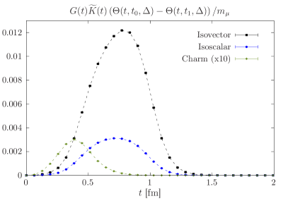
Figure 1: Integrands used to compute the intermediate window $a_{\mu}^{\rm win}$ for the isovector, isoscalar and charm quark contributions. The isoscalar contribution does not include the charm quark contribution. The data has been obtained on ensemble E250, which has close-to-physical quark masses, using two local vector currents and set 1 of renormalization and improvement coefficients.

Our simulations are performed in boxes of finite volume $L^{3}$ with $m_{\pi}L\gtrsim 4$, and corrections due to finite-size effects (FSE) are added to each ensemble individually prior to any continuum and chiral extrapolation. This is the only correction applied to the raw lattice data. FSE are dominated by the $\pi\pi$ channel and mostly affect the isovector correlator at large Euclidean times. For the intermediate window observable, they are highly suppressed compared to the full hadronic vacuum polarization contribution. Despite this suppression, FSE in the isovector channel are not negligible and require a careful treatment. They are of the same order of magnitude as the statistical precision for our most chiral ensemble and enhanced at larger pion masses. In the isoscalar channel, FSE are included only at the SU(3)_f point where $m_{\pi}=m_{K}$. The methodology is presented in Appendix C, and the corrections we have applied to the lattice data are given in the last column of Tables 6 and 5 respectively for Strategy 1 and 2. In our analysis, we have conservatively assigned an uncertainty of 25% to these finite-size corrections, in order to account for any potential effect not covered by the theoretical approaches described in Appendix C. In addition to the ensembles H105 and H200 that are only used to cross-check the FSE estimate, ensembles S400 and N302 are also affected by large finite-volume corrections. We exclude those ensembles in the isovector channel.

IV Extrapolation to the physical point

IV.1 Definition of the physical point in iso-symmetric QCD

Our gauge ensembles have been generated in the isospin limit of QCD with $m_{l}\equiv m_{u}=m_{d}$, neglecting strong isospin-breaking effects and QED corrections. Naively, those effects are expected to be of order ${\rm O}((m_{d}-m_{u})/\Lambda_{\rm QCD})\approx 1\%$ and ${\rm O}(\alpha)\approx 1\%$, and are not entirely negligible at our level of precision. In Ref. Budapest-Marseille-Wuppertal:2017okr , although the authors used a different scheme to define their iso-symmetric setup, those corrections have been found to be of the order of 0.4% for this window observable. A similar conclusion was reached in Ref. Blum:2018mom although only a subset of the diagrams was considered. This correction will be discussed in Section VI. Only in full QCD+QED is the precise value of the observable unambiguously defined: the separation between its iso-symmetric value and the isospin-breaking correction is scheme dependent. In Section IV.4, we provide the necessary information to translate our result into a different scheme.

Throughout our calculation, we define the ‘physical’ point in the $(m_{\pi},m_{K})$ plane by imposing the conditions Lellouch:discussion2021workshop ; Neufeld:1995mu ; Urech:1994hd

$$m_{\pi} = (m_{\pi^{0}})_{\rm phys},$$ (17)

$$2m^{2}_{K}-m^{2}_{\pi} = (m^{2}_{K^{+}}+m^{2}_{K^{0}}-m^{2}_{\pi^{+}})_{\rm phys}.$$ (18)

Inserting the PDG values Tanabashi:2018oca on the right-hand side, our physical iso-symmetric theory is thus defined by the values

$$m_{\pi}=134.9768(5)~{}{\rm{MeV}}\,,\quad m_{K}=495.011(10)~{}{\rm{MeV}}\,.$$ (19)

We note that since our gauge ensembles have been generated at constant sum of the bare quark masses, the linear combination $(m_{K}^{2}+m_{\pi}^{2}/2)$ is approximately constant. Two different strategies are used to extrapolate the lattice data to the physical point.

Strategy 1

We use the gradient flow observable $t_{0}$ Luscher:2010iy as an intermediate scale and the dimensionless parameters

$$\Phi_{2}=8t_{0}m_{\pi}^{2},\qquad\Phi_{4}=8t_{0}(m_{K}^{2}+{\textstyle\frac{1}{2}}m_{\pi}^{2})$$ (20)

as proxies for the light and the average quark mass as the physical point is approached. In the expressions of $\Phi_{2}$ and $\Phi_{4}$, $t_{0}$ is the pion- and kaon-mass dependent flow observable; we use the notation $t_{0}^{\rm sym}$ to denote its value at the SU(3)_f-symmetric point. We adopt the physical-point value $\sqrt{8t_{0}}=0.4081(20)(37)$ fm from Ref. Strassberger:2021tsu , obtained by equating the linear combination of pseudoscalar-meson decay constants

$$f_{K\pi}=\frac{2}{3}\Big{(}f_{K}+\frac{1}{2}f_{\pi}\Big{)}$$ (21)

to its physical value, set by the PDG values of the decay constants given below. Ref. Strassberger:2021tsu is an update of the work presented in Bruno:2016plf and includes a larger set of ensembles, including ensembles close to the physical point. We note that in Refs. Strassberger:2021tsu ; Bruno:2016plf the absolute scale was determined assuming a slightly different definition of the physical point: the authors used the meson masses corrected for isospin-breaking effects as in Aoki:2016frl , $m_{\pi}=134.8(3)$ MeV and $m_{K}=494.2(3)$ MeV. Using the NLO $\chi$PT expressions, we have estimated the effect on $f_{K\pi}$ of these small shifts in the target pseudoscalar meson masses to be at the sub-permille level and therefore negligible for our present purposes.

Strategy 2

Here we use $f_{\pi}$-rescaling, which was already presented in our previous work Gerardin:2019rua , and express all dimensionful quantities in terms of the ratio $f_{\pi}^{\rm phys}/(af_{\pi}^{\rm lat})$, where $af_{\pi}^{\rm lat}$ can be computed precisely on each ensemble. In this case, the intermediate scale $t_{0}$ is not needed and we use the following dimensionless proxies for the quark masses,

$$\widetilde{y}=\frac{m_{\pi}^{2}}{8\pi f_{\pi}^{2}},\qquad y_{K\pi}=\frac{m_{K}^{2}+\frac{1}{2}m_{\pi}^{2}}{8\pi f_{K\pi}^{2}}.$$ (22)

As $\Phi_{4}$, the proxy $y_{K\pi}$ is approximately constant along our chiral trajectory. Since all relevant observables have been computed as part of this project, this method has the advantage of being fully self-consistent, and all correlations can be fully propagated. It will be our preferred strategy. We use the following input to set the scale in our iso-symmetric theory Tanabashi:2018oca ; Aoki:2021kgd ,

$$f_{\pi}=130.56(14)~{}{\rm{MeV}}\,.$$ (23)

The quantity $y_{K\pi}$ is only used to correct for a small departure of the CLS ensembles from the physical value of this quantity, which we obtain using $f_{K}=157.2(5)~{}{\rm{MeV}}$ Tanabashi:2018oca ; Aoki:2021kgd . The latter, phenomenological value of $f_{K}$ implies a ratio $f_{K}/f_{\pi}$ that is consistent with the latest lattice determinations Bazavov:2017lyh ; Miller:2020xhy ; ExtendedTwistedMass:2021qui . The impact of the uncertainty of $f_{K}$ on $a_{\mu}^{\mathrm{win}}$ is small, $\delta a_{\mu}^{\mathrm{win}}\simeq 0.10\times 10^{-10}$, and occurs mainly through the strange contribution. In the isosymmetric theory, we take the phenomenological values of the triplet $(m_{\pi},m_{K},f_{\pi})$ as part of the definition of the target theory, and therefore only include the uncertainty from $f_{K}$ in our results. By contrast, in the final result including isospin-breaking effects, which we compare to a data-driven determination of $a_{\mu}^{\mathrm{win}}$, we include the experimental uncertainties of all quantities used as input.

The observables $m_{\pi}$, $m_{K}$, $f_{\pi}$ and $f_{K}$, as well as $t_{0}/a^{2}$ have been computed on all gauge ensembles and corrected for finite-size effects Colangelo:2005gd . Their values for all ensembles are listed in Table 7.

IV.2 Fitting procedure

We now present our strategy to extrapolate the data to the physical point in our iso-symmetric setup. The ensembles used in this work have been generated such that the physical point is approached keeping

$$X_{K}=\{\Phi_{4},y_{K\pi}\}$$ (24)

approximately constant, where the two entries correspond respectively to Strategy 1 and 2. To account for the small mistuning, only a linear correction in $\Delta X_{K}=X_{K}^{\rm phys}-X_{K}$ is thus considered. To improve the fit quality, a dedicated calculation of the dependence of $a_{\mu}^{\mathrm{win}}$ on $X_{K}$ has been performed, which is described in Appendix A. This analysis does not yet include all ensembles in the final result, and hence we decided to not apply this correction ensemble-by-ensemble prior to the global extrapolation to the physical point. Instead, we have used $\Delta X_{K}$ to fix suitable priors on the fit parameter $\gamma_{0}$ in Eq. (26), which parametrizes the locally linear dependence on $X_{K}$. The values of these priors are given in Appendix A.

To describe the light quark dependence beyond the linear term in

$$X_{\pi}=\{\Phi_{2},\widetilde{y}\}\,$$ (25)

(respectively for Strategy 1 and 2), we allow for different fit ansätze encoded in the function $f_{\rm ch}(X_{\pi})$. The precise choice of $f_{\rm ch}$ is motivated on physical grounds and depends on the quark flavor. The specific forms will be discussed below. Since on-shell O($a$)-improvement has been fully implemented, leading discretization artefacts are expected to scale as $a^{2}/t_{0}$ up to logarithmic corrections Symanzik:1983dc ; Husung:2019ytz . In the case of the vacuum polarization function, a further logarithmic correction proportional to $a^{2}\log a$ was discovered in Ce:2021xgd . Contrary to standard logarithmic corrections, it does not vanish as the coupling $g_{0}$ goes to zero due to correlators being integrated over very short distances. However, the intermediate window strongly suppresses the short-distance contribution, so that we do not expect this source of logarithmic enhancement to be relevant here. However, in the absence of further information on the relevant exponents of $\log a$ in full QCD Husung:2019ytz , we still consider a possible logarithmic correction with unit exponent. Moreover, to check whether we are in the scaling regime, we consider higher order terms proportional to $a^{3}$. Finally, we also allow for a term $\propto X_{a}^{2}X_{\pi}$ that describes pion-mass dependent discretization effects of order $a^{2}$.

Thus, for each discretization of the vector correlator, the continuum and chiral extrapolation is done independently assuming the most general functional form

$$a_{\mu}^{\mathrm{win,}{\rm f}}(X_{a},X_{\pi},X_{K})=a_{\mu}^{\mathrm{win,}{\rm f}}(0,X_{\pi}^{\exp},X_{K}^{\exp})+\beta_{2}\,X_{a}^{2}+\beta_{3}\,X_{a}^{3}+\delta\,X_{a}^{2}X_{\pi}+\epsilon\,X_{a}^{2}\log X_{a}\\ +\gamma_{0}\left(X_{K}-X_{K}^{\rm phys}\right)+\gamma_{1}\,\left(X_{\pi}-X_{\pi}^{\exp}\right)+\gamma_{2}\left(f_{\rm ch}(X_{\pi})-f_{\rm ch}(X_{\pi}^{\exp})\right)\,,$$ (26)

where ‘f’ can be any flavor content and $X_{a}=a/\sqrt{t_{0}}$ parametrizes the lattice spacing. Despite the availability of data from six lattice spacings and more than twenty ensembles, trying to fit all parameters is not possible. Thus each analysis is duplicated by switching on/off the parameters $\beta_{3}$, $\delta$ and $\epsilon$ that control the continuum extrapolation. In addition, for each functional form $f_{\rm ch}$ of the chiral dependence, different analyses are performed by imposing cuts in the pion mass (no cut, $<400$ MeV, $<300$ MeV) and/or in the lattice spacing.

Since several different fit ansätze can be equally well motivated, we apply the model averaging method presented in Jay:2020jkz ; Djukanovic:2021cgp where the Akaike Information Criterion (AIC) is used to weight different analyses and to estimate the systematic error associated with the fit ansatz (see also 1100705 ; Borsanyi:2020mff ). Thus, to each analysis $(n)$ described above (defined by a specific choice of $f_{\rm ch}$, applying cuts in the pion mass or in the lattice spacing, and including or excluding terms proportional to $\beta_{3}$, $\delta$, $\epsilon$) we associate a weight $w_{n}$ given by

$$w_{n}=N\exp\left[-\frac{1}{2}\left(\chi^{2}+2k-2n\right)\right]$$ (27)

where $\chi^{2}$ is the minimum value of the chi-squared of the correlated fit, $k$ is the number of fit parameters and $n$ is the number of data points included in the fit. The normalization factor $N$ is such that the sum over all the analyses’ weights are equal to one. Each analysis is again duplicated by either using the local-local or the local-conserved correlators. For those analyses, we use a flat weight. Finally, when cuts are performed, some fits may have very few degrees of freedom, and hence we exclude all analyses that contain fewer than three degrees of freedom. The central value of an observable $\mathcal{O}$ is then obtained by a weighted average over all analyses

$$\bar{\mathcal{O}}=\sum_{n}w_{n}\mathcal{O}_{n}\,,$$ (28)

and our estimate of the systematic error associated with the extrapolation to the physical point is given by

$$(\delta\mathcal{O})_{\rm syst}^{2}=\sum_{n}w_{n}(\mathcal{O}_{n}-\bar{\mathcal{O}})^{2}\,.$$ (29)

The statistical error is obtained from the Jackknife procedure using the estimator defined by Eq. (28).

IV.3 The continuum extrapolation at the SU(3)_f-symmetric point

To reach sub-percent precision, a good control over the continuum limit is mandatory Ce:2021xgd ; Husung:2019ytz . As discussed below, it is one of the largest contributions to our total error budget. Thus, before presenting our final result at the physical point, we first demonstrate our ability to perform the continuum extrapolation. We have implemented three different checks: First, two discretizations of the vector correlator are used and the extrapolations to the physical point are done independently. Both discretizations are expected to agree within errors in the continuum limit. Physical observables computed using Wilson-clover quarks approach the continuum limit with a rate $\propto a^{2}$ once the action and all currents are non-perturbatively O($a$)-improved Luscher:1996sc . To check our ability to fully remove O($a$) lattice artefacts in the action and the currents, two independent sets of improvement coefficients are used: both of them should lead to an $a^{2}$ scaling behavior but might differ by higher-order corrections. Finally, we have included six lattice spacings at the SU(3)_f-symmetric point, all of them below $0.1$ fm and down to 0.039 fm, to scrutinize the continuum extrapolation. In this section, we discuss those three issues, with a specific focus on the ensembles with SU(3)_f symmetry.

Ensembles with six different lattice spacings in the range $[0.039:0.099]$ fm are available for $m_{\pi}=m_{K}\approx 420~{}$MeV. Since the pion masses do not match exactly, we first describe our procedure to interpolate our SU(3)_f-symmetric ensembles to a single value of $X_{\pi}=X_{\pi}^{\star}$, to be be able to focus solely on the continuum extrapolation. This reference point $X_{\pi}^{\star}$ is chosen to minimize the quadratic sum of the shifts $\delta X_{\pi}=X_{\pi}-X_{\pi}^{\star}$.

We start by applying the finite-size effect correction discussed in the previous section to all ensembles. Then, a global fit over all the ensembles and simultaneously over both discretizations of the correlation function is performed using the functional form of Eq. (26) without any cut in the pion mass. Thus $(\gamma_{0},\gamma_{1},\gamma_{2})$ are fit parameters common to both discretizations, while the others are discretization-dependent. For the isovector contribution, we use the choice $f_{\rm ch}(X_{\pi})=1/X_{\pi}$ that leads to a reasonable $\chi^{2}/\mathrm{d.o.f.}=1.1$. The good $\chi^{2}$, and more importantly the good description of the light-quark mass dependence, ensures that the small interpolation to $X_{\pi}^{\star}$ is safe and that we do not bias the result. In practice, we have checked explicitly that using different functional forms $f_{\rm ch}$ to interpolate the data leads to changes that are small compared to the statistical error. Thus, for both choices of the improvement coefficients (set 1 and set 2), and for both discretizations LL and CL, the data from an SU(3)_f-symmetric ensemble is corrected in the pseudoscalar masses to the reference SU(3)_f-symmetric point at the same lattice spacing. The correction is obtained by taking the difference of Eq. (26) evaluated with the reference-point arguments $(X_{a},X^{\star}_{\pi},X_{K}^{\star})$ and the ensemble arguments $(X_{a},X_{\pi},X_{K})$, resulting in

$$a_{\mu}^{\mathrm{win,}{\rm f}}{}^{,\alpha}(X_{a},X^{\star}_{\pi},X_{K}^{\star})=a_{\mu}^{\mathrm{win,}{\rm f}}{}^{,\alpha}(X_{a},X_{\pi},X_{K})-\delta\,X_{a}^{2}\left(X_{\pi}-X_{\pi}^{\star}\right)-\gamma_{0}\left(X_{K}-X_{K}^{\star}\right)\\ -\gamma_{1}\,\left(X_{\pi}-X_{\pi}^{\star}\right)-\gamma_{2}\left(f_{\rm ch}(X_{\pi})-f_{\rm ch}(X_{\pi}^{\star})\right)\,,$$ (30)

where $\alpha=({\scriptsize\rm LL}),({\scriptsize\rm CL})$ stands for the discretization. Note that $X_{K}^{\star}=X_{\pi}^{\star}$ and $X_{K}=X_{\pi}$ in view of the SU(3)_f-symmetry. Throughout this procedure, correlations are preserved via the Jackknife analysis.

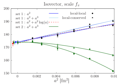
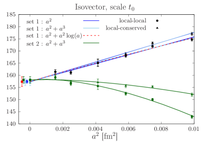
Figure 2: Continuum extrapolation for the isovector quark contribution at the SU(3)_f-symmetric point. Left: using $f_{\pi}$-rescaling. Right: with $t_{0}$ to set the scale. The blue and green points correspond to the two different sets of improvement coefficients (see Section III). For clarity, the extrapolated results have been shifted to the left.

In a second step, we extrapolate both discretizations of the correlation function to a common continuum limit, using data at all six lattice spacings and assuming a polynomial in the lattice spacing,

$$a_{\mu}^{\mathrm{win,}{\rm f}}{}^{,\alpha}(X_{a},X_{\pi}^{\star})=a_{\mu}^{\mathrm{win,}{\rm f}}(0,X_{\pi}^{\star})\left(1+\beta^{(\alpha)}_{2}\,X_{a}^{2}+\beta^{(\alpha)}_{3}\,X_{a}^{3}\right).$$ (31)

The two data sets obtained using the two different sets of improvement coefficients are fitted independently. The results are displayed in Fig. 2 for two cases: either applying $f_{\pi}$-rescaling (left panel) or using $t_{0}$ to set the scale (right panel). For Set 1 of improvement coefficients, we observe a remarkably linear behavior over the whole range of lattice spacings, whether $f_{\pi}$-rescaling is applied or not. The second set of improvement coefficients (Set 2) leads to some visible curvature, but the continuum limit is perfectly compatible provided that lattice artefacts of order $a^{3}$ are included in the fit.

We also tested the possibility of logarithmic corrections assuming the ansatz

$$a_{\mu}^{\mathrm{win,}{\rm f}}{}^{,\alpha}(X_{a},X_{\pi}^{\star})=a_{\mu}^{\mathrm{win,}{\rm f}}(0,X_{\pi}^{\star})\left(1+\beta^{(\alpha)}_{2}\,X_{a}^{2}+\epsilon^{(\alpha)}\,X_{a}^{2}\log X_{a}\right),$$ (32)

which is shown as the red symbol and red dashed curve in Fig. 2. The result is again compatible with the naive $a^{2}$ scaling, albeit with larger error. We conclude that logarithmic corrections are too small to be resolved in the data. We also remark that it is difficult to judge the quality of the continuum extrapolation based solely on the relative size of discretization effects between our coarsest and finest lattice spacing, as this measure strongly depends on the definition of the improvement coefficients.

We tested the modification of the continuum extrapolation via $X_{a}^{2}\rightarrow(\alpha_{\mathrm{s}}(1/X_{a}))^{\hat{\Gamma}}X_{a}^{2}$ as proposed in Refs. Husung:2019ytz ; Husung:2021mfl for $a_{\mu}^{\mathrm{win,I1}}$ and $a_{\mu}^{\mathrm{win,I0}}{}^{,c\!\!\!/}$ in our preferred setup, using $f_{\pi}$-rescaling and set 1 of improvement coefficients. The strong coupling constant $\alpha_{\mathrm{s}}$ has been obtained from the three-flavor $\Lambda$ parameter of Ref. Bruno:2017gxd . Several choices of $\hat{\Gamma}$ in the range from $0.76$ to $3$ were tested. The curvature that is introduced by this modification, especially for larger values of $\hat{\Gamma}$, would lead to larger values of $a_{\mu}^{\mathrm{win}}$ in the continuum limit. However, such curvature is not supported by the data, as indicated by a deterioration of the fit quality when $\hat{\Gamma}$ is increased. Therefore, only small weights would be assigned to such fits in our model averaging procedure, where the modification has not been included.

IV.4 Results for the isospin and flavor decompositions

Having studied the continuum limit at the SU(3)_f-symmetric point, we are ready to present the result of the extrapolation to the physical point. The charm quark contribution is not included here and will be considered separately in Section V.

For the isovector or light quark contribution we use the same set of functional forms as in Gerardin:2019rua $f_{\rm ch}(X_{\pi})=\{\log X_{\pi}\,;X_{\pi}^{2}\,;1/X_{\pi}\,;X_{\pi}\log X_{\pi}\}$. The data shows some small curvature close to the physical pion mass. Thus, the variation $f_{\rm ch}=0$ is excluded as it would significantly undershoot our ensemble at the physical pion mass (E250). We use Set 1 of improvement coefficients as our preferred choice and will use Set 2 only as a crosscheck. A typical extrapolation using $f_{\rm ch}(\widetilde{y})=1/\widetilde{y}$ without any cut in the data is shown in the left panel of Fig. 3. We find that the specific functional form of $f_{\rm ch}$ has much less impact on the extrapolation as compared to the inclusion of higher-order lattice artefacts. For the isoscalar and strange quark contributions, we restrict ourselves to functions that are not singular in the chiral limit: $f_{\rm ch}(X_{\pi})=\{0\,;X_{\pi}^{2}\,;X_{\pi}\log X_{\pi}\}$. Again, the extrapolation using $f_{\rm ch}(\widetilde{y})=\widetilde{y}\log\widetilde{y}$ with $\delta\neq 0$ and without any cut in the data is shown in the right panel of Fig. 3.

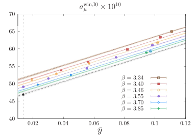
Figure 3: Left: one typical extrapolation of the isovector contribution using $f_{\rm ch}(\widetilde{y})=1/\widetilde{y}$. The data corresponds to the local-conserved discretization of the correlator using the set 1 of improvement coefficients. Error bands are the results from the fit for each of the six lattice spacings. The black line is the chiral extrapolation in the continuum limit. The black point is the result at the physical point. Right: same for the isoscalar contribution but using $f_{\rm ch}(\widetilde{y})=0$.

Using the fit procedure described above, the AIC estimator defined in Eq. (28) leads to the following results for the isovector ($I=1$) and the isoscalar contribution, charm excluded,

$$a_{\mu}^{\mathrm{win,I1}} =(186.30\pm 0.75_{\mathrm{stat}}\pm 1.08_{\mathrm{syst}})\times 10^{-10}\,,$$ (33)

$$a_{\mu}^{\mathrm{win,I0}}{}^{,c\!\!\!/} =(47.41\pm 0.23_{\mathrm{stat}}\pm 0.29_{\mathrm{syst}})\times 10^{-10}\,,$$ (34)

where the first error is statistical and the second is the systematic error from the fit form used to extrapolate our data to the physical point. In Table 2 , we also provide the derivatives

$$X\frac{\partial a_{\mu}^{\mathrm{win,}{\rm f}}}{\partial X}\,,\quad X\in\{m_{\pi},m_{K},f_{\pi},f_{K}\}\,,\quad{\rm f}\in\{\mathrm{I1},\mathrm{I0}\}\,,$$ (35)

to translate our result to a different iso-symmetric scheme.

We also note that both discretizations of the vector correlator yield perfectly compatible results. For the isovector contribution, and in units of $10^{-10}$, we obtain $186.14(0.87)_{\mathrm{stat}}(1.29)_{\mathrm{syst}}$ for the local-local discretization and $186.47(0.79)_{\mathrm{stat}}(0.79)_{\mathrm{syst}}$ for the local-conserved discretization, with a correlated difference of $-0.33(0.72)$. For the isoscalar contribution, we find $47.39(0.24)_{\mathrm{stat}}(0.36)_{\mathrm{syst}}$ for the local-local discretization and $47.43(0.20)_{\mathrm{stat}}(0.19)_{\mathrm{syst}}$ for the local-conserved discretization, with a correlated difference of $-0.04(0.10)$.

As an alternative to the fit weights given by Eq. (27), we have tried applying the weight factors used in Ref. Borsanyi:2020mff ; see the footnote below Eq. (27). While a major change occurs in the subset of fits that dominate the weighted average, the results do not change significantly. In particular, the central value of the isovector contribution changes by no more than half a standard deviation.

Table 2: Derivatives of the window quantity $a_{\mu}^{\rm win}$ (in units of $10^{-10}$), for both the isovector and isoscalar contributions, as defined by Eq. (35).

$X$	$m_{\pi}$	$m_{\rm K}$	$f_{\pi}$	$f_{\rm K}$
I1	$-7(5)$	$-11(7)$	$-66(84)$	7(5)
I0	2(1)	$-34(2)$	$-29(9)$	25(2)

Finally, we have also performed an extrapolation to the physical point using the second set of improvement coefficients. Since our study at the SU(3)_f-symmetric point shows curvature in the data, we exclude those continuum extrapolations that are only quadratic in the lattice spacing. The other variations are kept identical to those used for the first set. The results are slightly larger but compatible within one standard deviation. A comparison between the two strategies to set the scale and the two sets of improvement coefficients is shown in Fig. 4 for both the isovector and isoscalar contributions.

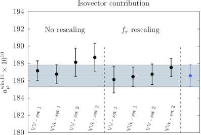
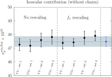
Figure 4: Comparison of the isovector and isoscalar contributions (without the charm) using different variations (either using $f_{\pi}$ or $t_{0}$ to set the scale, and with both sets of improvement coefficients). The blue point is our final estimate obtained from the rescaling method with the set 1 of improvement coefficients.

In order to facilitate comparisons with other lattice collaborations, we also present results for the light, strange and disconnected contributions separately. For the light and strange-quark connected contributions, we obtain

$$a_{\mu}^{\mathrm{win,ud}} =(207.00\pm 0.83_{\mathrm{stat}}\pm 1.20_{\mathrm{syst}})\times 10^{-10},$$ (36)

$$a_{\mu}^{\mathrm{win,s}} =(27.68\pm 0.18_{\mathrm{stat}}\pm 0.22_{\mathrm{syst}})\times 10^{-10}.$$ (37)

For the disconnected contribution, the correlation function is very precise in the time range relevant for the intermediate window, and a simple sum over lattice points is used to evaluate Eq. (5). The data are corrected for finite-size effects using the method described in Section C. Since our ensembles follow a chiral trajectory at fixed bare average quark mass, we can consider $a_{\mu}^{\mathrm{win,disc}}$ as being, to a good approximation, a function of the SU(3)_f-breaking variable $\Delta_{2}=\{8t_{0}(m_{K}^{2}-m_{\pi}^{2}),\;(m_{K}^{2}-m_{\pi}^{2})/(8\pi f_{K\pi}^{2})\}$ (respectively for Strategy 1 and 2), with the additional constraint that the disconnected contribution vanishes quadratically in $\Delta_{2}$ for $\Delta_{2}\to 0$. We apply the following ansatz

$$a_{\mu}^{\mathrm{win,disc}}(X_{a},X_{\pi},X_{K})=\Delta_{2}^{2}\left(\alpha+\gamma_{0}\left(X_{K}-X_{K}^{\rm phys}\right)+\beta_{2}X_{a}^{2}\right)\\ +\gamma_{1}\left(\frac{1}{X_{K}^{\rm phys}-\Delta_{2}}-\frac{\Delta_{2}}{(X_{K}^{\rm phys})^{2}}-\frac{1}{X_{K}^{\rm phys}}\right).$$ (38)

The ensembles close to the SU(3)_f symmetric point ($m_{\pi}\approx 350$ MeV) are affected by significant FSE corrections and are not included in the fit. We obtain for the disconnected contribution

$$a_{\mu}^{\mathrm{win,disc}}=(-0.81\pm 0.04_{\mathrm{stat}}\pm 0.08_{\mathrm{syst}})\times 10^{-10}\,,$$ (39)

and the extrapolation is shown in Fig. (5). The extrapolation using $t_{0}$ to set the scale shows less curvature close to the physical point. We use half the difference between the two extrapolations as our estimate for the systematic error. It is worth noting that the value for the intermediate window represents roughly 6% of the total contribution to $a_{\mu}^{\mathrm{hvp,disc}}$. As a crosscheck, we note that using Eqs. (36), (37) and (39) we would obtain $a_{\mu}^{\mathrm{win,I0}}{}^{,c\!\!\!/}=(47.57\pm 0.20_{\mathrm{stat}}\pm 0.26_{\mathrm{syst}})\times 10^{-10}$, in good agreement with Eq. (34).

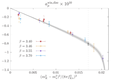
Figure 5: Extrapolation to the physical point for the quark-disconnected contribution using Eq. (38). The vertical dashed line represents the physical point in our iso-symmetric QCD setup. The black point is the result of the extrapolation, and the grey band represents the extrapolation to the continuum limit with $X_{K}=X_{K}^{\star}$. Points with dashed error bars are not included in the fit.

V The charm quark contribution

In our calculation, charm quarks are introduced in the valence sector only. A model estimate of the resulting quenching effect is provided in Appendix D. The method used to tune the mass of the charm quark has previously been described in Ref. Gerardin:2019rua and has been applied to additional ensembles in this work. We only sketch the general strategy here, referring the reader to Ref. Gerardin:2019rua for further details. For each gauge ensemble, the mass of the ground-state $c\bar{s}$ pseudoscalar meson is computed at four values of the charm-quark hopping parameter. Then the value of $\kappa_{c}$ is obtained by linearly interpolating the results in $1/\kappa_{c}$ to the physical $D_{s}$ meson mass $m_{D_{s}}=1968.35(0.07)$ MeV Tanabashi:2018oca . We have checked that using either a quadratic fit or a linear fit in $\kappa_{c}$ leads to identical results at our level of precision. The results for all ensembles are listed in the second column of Table 10.

The renormalization factor $\hat{Z}_{V}^{(c)}$ of the local vector current has been computed non-perturbatively on each individual ensemble by imposing the vector Ward-identity using the same setup as in Ref. Gerardin:2018kpy , but with a charm spectator quark. To propagate the error from the tuning of $\kappa_{c}$, both $\hat{Z}_{V}^{(c)}$ and $a_{\mu}^{\mathrm{win,c}}$ are computed at three values of $\kappa$ close to $\kappa_{c}$. In the computation of correlation functions, the same stochastic noises are used to preserve the full statistical correlations. For both quantities, we observe a very linear behavior and a short interpolation to $\kappa_{c}$ is performed. The systematic error introduced by the tuning of $\kappa_{c}$ is propagated by computing the discrete derivatives of both observables with respect to $\kappa_{c}$ (second error quoted in Table 10). This systematic error is considered as uncorrelated between different ensembles.

From ensembles generated with the same bare parameters but with different spatial extents (H105/N101 or H200/N202), it is clear that FSE are negligible in the charm-quark contribution. As in our previous work Gerardin:2019rua , the local-local discretization exhibits a long continuum extrapolation with discretization effects as large as 70% between our coarsest lattice spacing and the continuum limit, compared to only 12% for the local-conserved discretization. Thus, we discard the local-local discretization from our extrapolation to the physical point, which assumes the functional form

$$a_{\mu}^{\mathrm{win,c}}(X_{a},X_{\pi},X_{K})=a_{\mu}^{\mathrm{win,c}}(0,X_{\pi}^{\exp},X_{K}^{\exp})+\beta_{2}\,X_{a}^{2}+\beta_{3}\,X_{a}^{3}+\delta\,X_{a}^{2}X_{\pi}+\beta_{4}\,X_{a}^{2}\log(X_{a})\\ +\gamma_{0}\left(X_{K}-X_{K}^{\rm phys}\right)+\gamma_{1}\,\left(X_{\pi}-X_{\pi}^{\exp}\right)\,.$$ (40)

Lattice artefacts are described by a polynomial in $X_{a}=a/\sqrt{t_{0}^{\rm sym}}$ and a possible logarithmic term is included; recall that $t_{0}^{\rm sym}$ denotes the value of the flow observable at the SU(3)_f-symmetric point. Only the set of proxies $X_{\pi}=\phi_{2}$ and $X_{K}=\phi_{4}$ is used. The light-quark dependence shows a very flat behavior, and a good $\chi^{2}/\mathrm{d.o.f.}=0.9$ is obtained without any cut in the pion mass. The corresponding extrapolation is shown on the right panel of Fig. 6.

Before quoting our final result, we provide strong evidence that our continuum extrapolation is under control by looking specifically at the SU(3)_f-symmetric point where six lattice spacings are available. As for the isovector contribution, we use Eq. (40) to correct for the small pion-mass mistuning at the SU(3)_f-symmetric point. The data are interpolated to a single value of $X_{\pi}^{*}$ using the same strategy as in Eq. (30). Those corrected points are finally extrapolated to the continuum limit using the ansatz (31). The result is shown in the left panel of Fig. 6 for the two sets of improvement coefficients of the vector current. Again, excellent agreement is observed between the two data sets. Even for the charm-quark contribution, we observe very little curvature when using the set 1 of improvement coefficients.

Having confirmed that our continuum extrapolation is under control, we quote our final result for the charm contribution obtained using the ansatz (40). Using Eq. (28), the AIC analysis described above leads to

$$a_{\mu}^{\mathrm{win,c}}=(2.89\pm 0.03_{\mathrm{stat}}\pm 0.03_{\mathrm{syst}}\pm 0.13_{\rm scale})\times 10^{-10}\,,$$ (41)

where variations include cuts in the pion masses and in the lattice spacing, and fits where the parameters $\beta_{3}$, $\beta_{4}$ and $\delta$ have been either switched on or off.

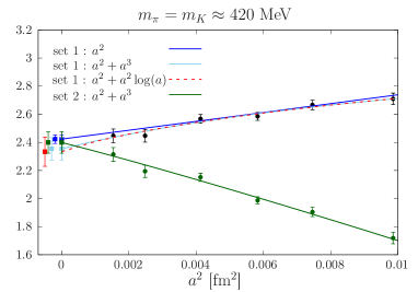
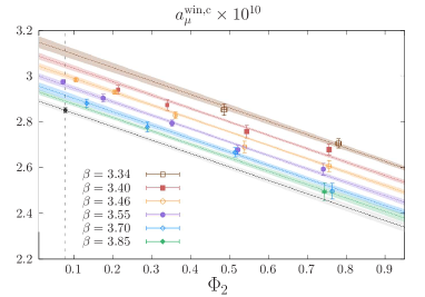
Figure 6: Left panel: study of the continuum extrapolation of the charm quark contribution to $a_{\mu}^{\rm win}$ at the SU$(3)_{\rm f}$-symmetric point using the local-conserved discretization of the correlation function. The black and green points are obtained using two independent sets of improvement coefficients, as explained in Section III.2. Right panel: Example of a typical extrapolation to the physical point of the charm-quark contribution. The error from the scale setting, which is highly correlated between ensembles, is not shown. The plain lines are obtained from the fit function (40) without any cut in the pion mass.

VI Isospin breaking effects

As discussed in the previous Sections III and IV.1, our computations are performed in an isospin-symmetric setup, neglecting the effects due to the non-degeneracy of the up- and down-quark masses and QED. At the percent and sub-percent level of precision it is, however, necessary to consider the impact of isospin-breaking effects. To estimate the latter, we have computed $a_{\mu}^{\mathrm{win}}$ in QCD+QED on a subset of our isospin-symmetric ensembles using the technique of Monte Carlo reweighting Ferrenberg:1988yz ; Duncan:2004ys ; Hasenfratz:2008fg ; Finkenrath:2013soa ; deDivitiis:2013xla combined with a leading-order perturbative expansion of QCD+QED around isosymmetric QCD in terms of the electromagnetic coupling $e^{2}$ as well as the shifts in the bare quark masses $\Delta m_{u},\Delta m_{d},\Delta m_{s}$ deDivitiis:2013xla ; Risch:2021hty ; Risch:2019xio ; Risch:2018ozp ; Risch:2017xxe . Consequently, we must evaluate additional diagrams that represent the perturbative quark mass shifts as well as the interaction between quarks and photons. We make use of non-compact lattice QED and regularize the manifest IR divergence with the QED_L prescription Hayakawa:2008an , with the boundary conditions of the photon and QCD gauge fields chosen in accordance Risch:2018ozp . We characterize the physical point of QCD+QED by the quantities $m_{\pi^{0}}^{2}$, $m_{K^{+}}^{2}+m_{K^{0}}^{2}-m_{\pi^{+}}^{2}$, $m_{K^{+}}^{2}-m_{K^{0}}^{2}-m_{\pi^{+}}^{2}+m_{\pi^{0}}^{2}$ and the fine-structure constant $\alpha$ Risch:2021hty . The first three quantities are inspired by leading-order chiral perturbation theory including leading-order mass and electromagnetic isospin-breaking corrections Neufeld:1995mu , and correspond to proxies for the average light-quark mass, the strange-quark mass, and the light-quark mass splitting. As we consider leading-order effects only, the electromagnetic coupling does not renormalize deDivitiis:2013xla , i.e. we may set $e^{2}=4\pi\alpha$. The lattice scale is also affected by isospin breaking, which we however neglect at this stage. Making use of the isosymmetric scale Bruno:2016plf , we match $m_{\pi^{0}}^{2}$ and $m_{K^{+}}^{2}+m_{K^{0}}^{2}-m_{\pi^{+}}^{2}$ in both theories on each ensemble and set $m_{K^{+}}^{2}-m_{K^{0}}^{2}-m_{\pi^{+}}^{2}+m_{\pi^{0}}^{2}$ to its experimental value.

We have computed the leading-order QCD+QED quark-connected contribution to $a_{\mu}^{\mathrm{win}}$ as well as the pseudoscalar meson masses $m_{\pi^{0}}$, $m_{\pi^{+}}$, $m_{K^{0}}$ and $m_{K^{+}}$ required for the hadronic renormalization scheme on the ensembles D450, N200, N451 and H102, neglecting quark-disconnected diagrams as well as isospin-breaking effects in sea-quark contributions. The considered quark-connected diagrams are evaluated using stochastic U$(1)$ quark sources with support on a single timeslice whereas the all-to-all photon propagator in Coulomb gauge is estimated stochastically by means of $Z_{2}$ photon sources. Covariant approximation averaging Shintani:2014vja in combination with the truncated solver method Bali:2009hu is applied to reduce the stochastic noise. We treat the noise problem of the vector-vector correlation function at large time separations by means of a reconstruction based on a single exponential function. A more detailed description of the computation can be found in Refs. Risch:2021nfs ; Risch:2021hty ; Risch:2019xio . The renormalization procedure of the local vector current in the QCD+QED computation is based on a comparison of the local-local and the conserved-local discretizations of the vector-vector correlation function and hence differs from the purely isosymmetric QCD calculation Gerardin:2018kpy described in Section III.2. We therefore determine the relative correction by isospin breaking in the QCD+QED setup. For $f_{\pi}$-rescaling as introduced in Section IV.1, isospin-breaking effects in the determination of $f_{\pi}$ are neglected. We observe that the size of the relative first-order corrections for $a_{\mu}^{\mathrm{win}}$ is compatible on each ensemble and can in total be estimated as a $(0.3\pm 0.1)\%$ effect.

VII Final result and discussion

We first quote our final result $a_{\mu}^{\mathrm{win,iso}}$ in our iso-symmetric setup as defined in Section IV.1. Using the isospin decomposition, and combining Eqs. (33), (34) and (41), we find

$$a_{\mu}^{\mathrm{win,I1}} =(186.30\pm 0.75_{\mathrm{stat}}\pm 1.08_{\mathrm{syst}})\times 10^{-10}\,,$$ (42)

$$a_{\mu}^{\mathrm{win,I0}}=a_{\mu}^{\mathrm{win,I0}}{}^{,c\!\!\!/}+a_{\mu}^{\mathrm{win,c}} =(50.30\pm 0.23_{\mathrm{stat}}\pm 0.32_{\mathrm{syst}})\times 10^{-10}\,,$$ (43)

$$a_{\mu}^{\mathrm{win,iso}}=a_{\mu}^{\mathrm{win,I1}}+a_{\mu}^{\mathrm{win,I0}} =(236.60\pm 0.79_{\mathrm{stat}}\pm 1.13_{\mathrm{syst}}\pm 0.05_{\rm Q})\times 10^{-10}\,,$$ (44)

where the first error is statistical, the second is the systematic error, and the last error of $a_{\mu}^{\mathrm{win,iso}}$ is an estimate of the quenching effect of the charm quark derived in Appendix D. Overall, this uncertainty has a negligible effect on the systematic error estimate. The small bottom quark contribution has been neglected. For $a_{\mu}^{\mathrm{hvp}}$, this contribution has been computed in Colquhoun:2014ica and found to be negligible at the current level of precision.

As stressed in Section IV.1, our definition of the physical point in our iso-symmetric setup is scheme dependent. To facilitate the comparison with other lattice collaborations, the derivatives with respect to the quantities used to define our iso-symmetric scheme are provided in Table 2. They can be used to translate from one prescription to another a posteriori.

One of the main challenges for lattice calculations of both $a_{\mu}^{\rm hvp}$ and the window observable is the continuum extrapolation of the light quark contribution, which dominates the results by far. To address this specific point, we have used six lattice spacings in the range [0.039,0.0993] fm in our calculation, along with two different discretizations of the vector current (see the discussion in Section IV.3). Although this work contains many ensembles away from the physical pion mass, we observe only a mild dependence on the proxy used for the light-quark mass. This observation is corroborated by the fact that, in the model averaging analysis, most of the spread comes from fits that differ in the description of lattice artefacts rather than on the functional form $f_{\rm ch}$ that describes the light-quark mass dependence.

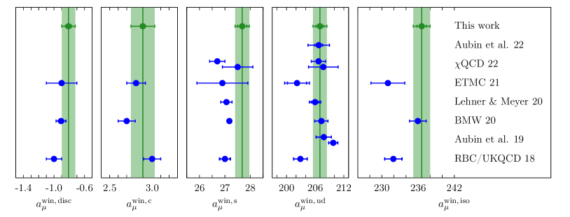
Figure 7: Comparison of our results (in units of $10^{-10}$) with other lattice calculations Blum:2018mom ; Aubin:2019usy ; Borsanyi:2020mff ; Lehner:2020crt ; Giusti:2021dvd ; Wang:2022lkq ; Aubin:2022hgm in isosymmetric QCD. The four panels on the left show compilations of the individual quark-disconnected, charm, strange and light quark contributions. The total result for $a_{\mu}^{\mathrm{win}}$ in the isosymmetric case is shown in the rightmost panel. Our results are represented by green circles and vertical bands.

In Fig. 7, we compare our results in the isosymmetric theory with other lattice calculations. Our estimate for $a_{\mu}^{\mathrm{win,iso}}$ agrees well with that of the BMW collaboration who quote $a_{\mu}^{\mathrm{win,iso}}=236.3(1.4)\times 10^{-10}$ using the staggered quark formulation Borsanyi:2020mff . However, our result is about $2.3\sigma$ above the published value by the RBC/UKQCD collaboration, $a_{\mu}^{\mathrm{win,iso}}=232.0(1.5)\times 10^{-10}$, obtained using domain wall fermions Blum:2018mom . It is also $1.7\sigma$ above the recent estimate quoted by ETMC, based on the twisted-mass formalism Giusti:2021dvd , which reads $a_{\mu}^{\mathrm{win,iso}}=231.0(2.8)\times 10^{-10}$. The difference with the latter two calculations can be traced to the light-quark contribution $a_{\mu}^{\mathrm{win,ud}}$, which is shown in the second panel from the right. In this context, it is interesting to note that, apart from BMW, two independent calculations using staggered quarks (albeit with a different action as compared to the BMW collaboration) have quoted results for $a_{\mu}^{\mathrm{win,ud}}$ Aubin:2019usy ; Aubin:2022hgm ; Lehner:2020crt that are in good agreement with our estimate, as can be seen in Fig. 7. The middle panel of the figure shows that our estimate for the strange quark contribution is slighly higher compared to other groups, but due to the relative smallness of $a_{\mu}^{\mathrm{win,s}}$ this cannot account for the difference between our result for $a_{\mu}^{\mathrm{win,iso}}$ and Refs. Giusti:2021dvd and Blum:2018mom . Good agreement with the BMW, ETMC and RBC/UKQCD collaborations is found for both the charm and quark-disconnected contributions.

If one accepts that most lattice estimates for the light-quark connected contribution $a_{\mu}^{\mathrm{win,ud}}$ have stabilized around $\approx 207\times 10^{-10}$, one may search for an explanation why the results by RBC/UKQCD Blum:2018mom and ETMC Giusti:2021dvd are smaller by about 2%. This is particularly important since $a_{\mu}^{\mathrm{win,ud}}$ contributes about 87% to the entire intermediate window observable. One possibility is that the extrapolations to the physical point in Refs. Blum:2018mom and Giusti:2021dvd are both quite long. For instance, the minimum pion mass among the set of ensembles used by ETMC is only about 220 MeV, while the result by RBC/UKQCD has been obtained from two lattice spacings, i.e. 0.084 fm and 0.114 fm. Further studies using additional ensembles at smaller pion mass and lattice spacings are highly desirable to clarify this important issue.

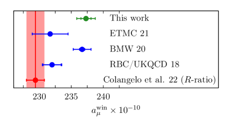
Figure 8: Comparison of our result for $a_{\mu}^{\mathrm{win}}$ including isospin-breaking corrections with the estimates by ETMC Giusti:2021dvd , BMW Borsanyi:2020mff and RBC/UKQCD Blum:2018mom . The estimate based on the data-driven method of Ref. Colangelo:2022vok is shown in red.

In order to compare our result with phenomenological determinations of the intermediate window observable, we must correct for the effects of isospin-breaking. Our calculation of isospin-breaking corrections, described in Section VI, has been performed on a subset of our ensembles and is, at this stage, lacking a systematic assessment of discretization and finite-volume errors. Furthermore, only quark-connected diagrams have been considered so far. To account for this source of uncertainty, we double the error and thereby apply a relative isospin-breaking correction of $(0.3\pm 0.2)\%$ to $a_{\mu}^{\mathrm{win,iso}}$, which amounts to a shift of $+(0.70\pm 0.47)\times 10^{-10}$. Thus, our final result including isospin-breaking corrections is

$$a_{\mu}^{\mathrm{win}}=(237.30\pm 0.79_{\mathrm{stat}}\pm 1.13_{\mathrm{syst}}\pm 0.05_{\rm Q}\pm 0.47_{\rm IB})\times 10^{-10}\,.$$ (45)

Adding all errors in quadrature yields $237.30(1.46)\times 10^{-10}$ which corresponds to a precision of 0.6%. A comparison with other lattice calculations is shown in Fig. 8. Since corrections due to isospin breaking are small, the same features are observed as in the isosymmetric theory: while our result agrees well with the published estimate from BMW Borsanyi:2020mff , it is larger than the values quoted by ETMC Giusti:2021dvd and RBC/UKQCD Blum:2018mom . Our result lies $3.9\sigma$ above the recent evaluation using the data-driven method Colangelo:2022vok , which yields $a_{\mu}^{\mathrm{win}}=229.4(1.4)\times 10^{-10}$ and is shown in red in Fig. 8. Our result for $a_{\mu}^{\mathrm{win}}$ is also consistent with the observation that the central value of our 2019 result for the complete hadronic vacuum polarization contribution Gerardin:2019rua lies higher than the phenomenology estimate, albeit with much larger uncertainties. In Ref. Ce:2022eix we observed a similar, but statistically much more significant enhancement in the hadronic running of the electromagnetic coupling, $\Delta\alpha_{\mathrm{had}}(-Q^{2})$ relative to the data-driven evaluation, especially for $Q^{2}\lesssim 3\,{\rm GeV}^{2}$. As pointed out at the end of Section II, the relative contributions from the three intervals of center-of-mass energy separated by $\sqrt{s}=600\,$MeV and $\sqrt{s}=900\,$MeV are similar for $a_{\mu}^{\mathrm{win}}$ and $\Delta\alpha_{\mathrm{had}}(-1{\rm GeV}^{2})$, even though the respective weight functions in the time-momentum representation are rather different. The fact that the lattice determination is larger by more than three percent for both quantities, in each case with a combined error of less than one percent, suggests that a genuine difference exists at the level of the underlying spectral function, $R(s)/(12\pi^{2})$, between lattice QCD and phenomenology.

If one were to subtract the data-driven evaluation of $a_{\mu}^{\mathrm{win}}$ from the White Paper estimate Aoyama:2020ynm and replace it by our result in Eq. (45), the tension between the SM prediction for $a_{\mu}$ and experiment would be reduced to $2.9\sigma$. This observation illustrates the relevance of the window observable for precision tests of the SM. Our findings also strengthen the evidence supporting a tension between data-driven and lattice determinations of $a_{\mu}^{\rm hvp}$.

In our future work we will extend the calculation to other windows and focus on the determination of the full hadronic vacuum polarization contribution, $a_{\mu}^{\rm hvp}$.

Appendix A Mistuning of the chiral trajectory

The ensembles used in our work have been generated with a constant bare average sea quark mass which differs from a constant renormalized mass by $\mathrm{O}(a)$ cutoff effects. When the sum of the renormalized quark masses is kept constant, the dimensionless parameters $\phi_{4}$ and $y_{K\pi}$, which have been introduced in Section IV.1 to define the chiral trajectories towards the physical point, are constant to leading order in chiral perturbation theory ($\chi$PT). Therefore, $\phi_{4}$ and $y_{K\pi}$ cannot be constant across our set of ensembles due to cutoff effects and higher-order effects from $\chi$PT.

We have to correct for the sources of mistuning of our ensembles with respect to the chiral trajectories of strategies 1 and 2. This can be done by parameterizing the dependence of our observables on $X_{K}\in\{y_{K\pi},\phi_{4}\}$ in the combined chiral-continuum extrapolation. However, since the pion and kaon masses are not varied independently within our set of ensembles, the dependence on $\Delta X_{K}=X_{K}^{\rm phys}-X_{K}$ cannot be resolved reliably in our fits. A different strategy has to be employed to stabilize our extrapolation to the physical point.

Explicit corrections of the mistuning prior to the chiral extrapolation have been used in Bruno:2016plf to approach the physical point at constant $\phi_{4}=\phi_{4}^{\mathrm{phys}}$. These corrections are based on small shifts defined from the first order Taylor expansion of the quark mass dependence of lattice observables. The expectation value of a shifted observable is given by

$$\langle\mathcal{O}\rangle\rightarrow\langle\mathcal{O}\rangle+\sum_{i=1}^{N_{\mathrm{f}}}\Delta m_{\mathrm{q},i}\frac{\mathrm{d}\langle\mathcal{O}\rangle}{\mathrm{d}m_{\mathrm{q},i}}\,,$$ (46)

with the $N_{\mathrm{f}}=3$ sea quark mass shifts $\Delta m_{\mathrm{q},i}$. Within this appendix, we work with observables and expectation values that are defined after integration over the fermion fields, i.e. the expectation values are taken with respect to the gauge configurations. The total derivative of an observable with respect to the quark masses is decomposed via

$$\frac{\mathrm{d}\langle\mathcal{O}\rangle}{\mathrm{d}m_{\mathrm{q},i}}=\left\langle\frac{\partial\mathcal{O}}{\partial m_{\mathrm{q},i}}\right\rangle-\left\langle\mathcal{O}\frac{\partial S}{\partial m_{\mathrm{q},i}}\right\rangle+\left\langle\mathcal{O}\right\rangle\left\langle\frac{\partial S}{\partial m_{\mathrm{q},i}}\right\rangle\,.$$ (47)

The partial derivative of an observable with respect to a quark mass of flavor $i$ captures the effect of shifts of valence quark masses. The second and third terms that contain the derivative of the action $S$ with respect to the quark masses account for sea quark effects. The chain rule is used to compute the derivatives of derived observables.

The chain rule relating the derivatives with respect to the quark masses to those with respect to the variables $X_{j}=X_{\pi},X_{K}$ can be written

$$\sum_{i=1}^{N_{\mathrm{f}}}n_{i}\;\frac{\mathrm{d}\langle{\cal O}\rangle}{\mathrm{d}m_{\mathrm{q},i}} =\sum_{j=\pi,K}\Delta_{j}(\vec{n})\,\frac{\mathrm{d}\langle\mathcal{O}\rangle}{\mathrm{d}X_{j}},\qquad\Delta_{j}(\vec{n})\equiv\sum_{i=1}^{N_{\mathrm{f}}}n_{i}\;\frac{\mathrm{d}X_{j}}{\mathrm{d}m_{\mathrm{q},i}}$$ (48)

$\forall\,\vec{n}=(n_{1},n_{1},n_{3})$, the condition $n_{1}=n_{2}$ being imposed to remain in the isosymmetric theory. In particular, if the direction of the vector $\vec{n}$ in the space of quark masses is chosen such that $\Delta_{\pi}(\vec{n})$ vanishes, the following expression Strassberger:2021tsu for the derivative of an observable with respect to $X_{K}$ is obtained,

$$\frac{\mathrm{d}\langle\mathcal{O}\rangle}{\mathrm{d}X_{K}}=\frac{1}{\Delta_{K}(\vec{n})}\sum_{i=1}^{N_{\mathrm{f}}}n_{i}\frac{\mathrm{d}\langle\mathcal{O}\rangle}{\mathrm{d}m_{\mathrm{q},i}}.$$ (49)

In Bruno:2016plf the shifts $n_{i}$ have been chosen to be degenerate for all three sea quarks. In Strassberger:2021tsu the same approach is taken at the $\mathrm{SU}(3)_{\rm f}$-symmetric point and $\vec{n}=(0,0,1)$ is used when $am_{{\rm q},l}\neq am_{{\rm q},s}$. To stabilize the predictions for the derivatives, they are modeled as functions of lattice spacing and quark mass.

To improve the reliability of our chiral extrapolation, we have determined the derivatives of $a_{\mu}^{\mathrm{win,ud}}$ and $a_{\mu}^{\mathrm{win,s}}$ with respect to light and strange quark masses on a large subset of the ensembles in Table 1. Whereas the computation of the first term in Eq. (47) shows a good signal for the vector-vector correlation function, the second and third term carry significant uncertainties. In the case of $f_{\pi}$-rescaling, a non-negligible statistical error that has its origin in ${\mathrm{d}f_{\pi}}/{\mathrm{d}m_{\mathrm{q},i}}$ enters the derivative of $a_{\mu}^{\mathrm{win}}$.

Our computation does not yet cover all ensembles in this work and has significant uncertainties on some of the included ensembles. Moreover, we have not computed the mass-derivative of $a_{\mu}^{\mathrm{win,disc}}$ that enters $a_{\mu}^{\mathrm{win,I0}}$. Therefore, we have decided not to correct our observables prior to the global extrapolation but to determine the coefficient $\gamma_{0}$ in Eq. (26) instead. We do not aim for a precise determination here but focus instead on the determination of a sufficiently narrow prior width, in order to stabilize the chiral-continuum extrapolation.

We compute the derivatives with respect to $X_{K}$ as specified in Eq. (49) with the shift vector $\vec{n}$ chosen such that $\Delta_{\pi}(\vec{n})$ vanishes ensemble by ensemble, i.e. the shift is taken in a direction in the quark mass plane where $X_{\pi}$ remains constant. The derivatives are therefore sensitive to shifts in the kaon mass. A residual shift of $X_{a}$ is present at the permille level.

We collect our results for the derivatives with respect to $\phi_{4}$ and $y_{K\pi}$ in Table 3. Throughout this appendix, we use units of $10^{-10}$ for $a_{\mu}^{\mathrm{win}}$, as well as for coefficient $\gamma_{0}$. The results are based on the local-local discretization of the correlation functions and the improvement coefficients and renormalization constants of set 1. As can be seen, the derivative of the isovector contribution to the window observable vanishes within error on most of the ensembles. This is expected from the order-of-magnitude estimate in Eq. (84). No clear trend regarding a dependence on $X_{\pi}$, $X_{K}$ or $X_{a}$ can be resolved. We show the derivative of $a_{\mu}^{\mathrm{win,I1}}$ with respect to $X_{\pi}$ in the upper panels of Fig. 9. For the corresponding priors for the chiral-continuum extrapolation we choose

$$\gamma_{0}^{{\mathrm{win,I1},y_{K\pi}}}=0(50)\qquad\gamma_{0}^{{\mathrm{win,I1},\phi_{4}}}=-2.5(5.0)\,.$$ (50)

The derivative of the strange-connected contribution of the window observable with respect to $X_{K}$ is negative and can be determined to good precision. Our results are shown in the lower panels of Fig. 9. We choose our priors such that their width encompasses the spread of the data. For the strange-connected and the isoscalar contribution, we choose

$$\gamma_{0}^{{\mathrm{win,s},y_{K\pi}}}=-100(20)\qquad\gamma_{0}^{{\mathrm{win,s},\phi_{4}}}=-12.5(2.5)\,.$$ (51)

These values are compatible with the estimate in Eq. (77).

Discretization effects in the data may be inspected by comparing the derivatives based on the two sets of improvement coefficients. Such effects are largest for the two ensembles at $\beta=3.34$, but are still smaller than the spread in the data and therefore not significant with respect to our prior widths. In our global extrapolations, we use a single set of priors irrespective of the improvement procedure.

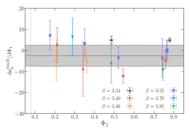
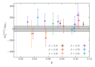
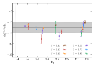
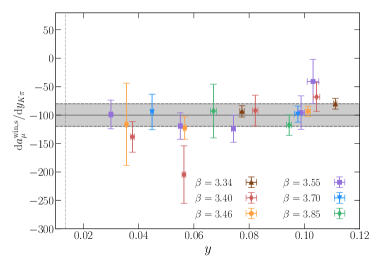
Figure 9: Derivatives of the isovector and the strange-connected contributions to the window observable with respect to $X_{\pi}$. The gray areas illustrate the priors that are used in the global extrapolation.

Table 3: Derivatives of the isovector and the strange-connected contributions to the window observable with respect to $X_{K}$ in units of $10^{-10}$. The data is based on the the local-local discretization of the vector-vector correlation function and the improvement coefficients of set 1.

id	$\frac{\mathrm{d}a_{\mu}^{\mathrm{win,I1}}}{\mathrm{d}\Phi_{4}}$	$\frac{\mathrm{d}a_{\mu}^{\mathrm{win,I1}}}{\mathrm{d}y_{K\pi}}$	$\frac{\mathrm{d}a_{\mu}^{\mathrm{win,s}}}{\mathrm{d}\Phi_{4}}$	$\frac{\mathrm{d}a_{\mu}^{\mathrm{win,s}}}{\mathrm{d}y_{K\pi}}$
A653	$\phantom{-}5.0(1.1)$	$\phantom{-}83(39)$	$-10.0(0.7)$	$-80(10)$
A654	$\phantom{-}5.0(1.9)$	$\phantom{-}96(47)$	$-11.3(0.5)$	$-93(10)$
H101	$-4.7(3.9)$	$\phantom{-}145(137)$	$-13.4(1.1)$	$-68(26)$
H102	$-12.2(3.5)$	$\phantom{-}46(118)$	$-14.5(1.0)$	$-91(27)$
N101	$-8.9(12.9)$	$-163(143)$	$-17.8(2.1)$	$-204(51)$
C101	$\phantom{-}2.6(8.3)$	$-84(93)$	$-12.1(1.6)$	$-138(27)$
B450	$-3.4(2.6)$	$\phantom{-}42(39)$	$-12.5(0.7)$	$-93(9)$
N451	$-5.3(5.2)$	$-68(71)$	$-12.8(0.5)$	$-122(20)$
D450	$-4.9(10.0)$	$-85(233)$	$-11.1(0.8)$	$-116(73)$
H200	$-0.3(5.3)$	$\phantom{-}241(198)$	$-10.8(1.3)$	$-40(40)$
N202	$-3.5(9.2)$	$\phantom{-}79(136)$	$-14.5(2.2)$	$-95(30)$
N203	$-3.5(5.1)$	$\phantom{-}125(106)$	$-16.5(1.6)$	$-123(25)$
N200	$\phantom{-}3.3(7.2)$	$\phantom{-}136(128)$	$-14.0(1.3)$	$-119(24)$
D200	$\phantom{-}7.1(7.1)$	$\phantom{-}121(93)$	$-11.8(1.4)$	$-98(26)$
N300	$\phantom{-}0.4(4.3)$	$\phantom{-}8(53)$	$-11.4(1.1)$	$-98(15)$
J303	$\phantom{-}6.5(9.1)$	$\phantom{-}197(148)$	$-13.4(1.2)$	$-94(32)$
J500	$-9.0(5.3)$	$-18(68)$	$-15.1(1.5)$	$-117(19)$
J501	$-6.1(9.4)$	$\phantom{-}88(189)$	$-12.5(3.0)$	$-92(48)$

Appendix B Phenomenological models

In the first subsection of this appendix, we collect estimates of the sensitivity of the window observables to various intervals in $\sqrt{s}$ in the dispersive approach. The observable $a_{\mu}^{\mathrm{win}}$ can indeed be obtained from experimental data for the ratio $R(s)$ defined in Eq. (10) via

$$a_{\mu}^{\mathrm{win}} = \int_{0}^{\infty}ds\,f_{\rm win}(s)\,R(s),$$ (52)

where the weight function is given by

$$f_{\rm win}(s) = \frac{\alpha^{2}\,\sqrt{s}}{24\pi^{4}}\int_{0}^{\infty}dt\;e^{-t\sqrt{s}}\widetilde{K}(t)\,[\Theta(t,t_{0},\Delta)-\Theta(t,t_{1},\Delta)]\ .$$ (53)

In practice, since the integrand is very strongly suppressed beyond 1.5 fm, we have used the short-distance expansion of $\widetilde{K}(t)$ given by Eq. (B16) of Ref. DellaMorte:2017dyu , which is very accurate up to 2 fm.

The second and the third subsection contain phenomenological estimates of the derivatives of the strangeness and the isovector contributions to $a_{\mu}^{\rm win}$ with respect to the kaon mass at fixed pion mass, as a cross-check of the lattice results presented in Appendix A.

B.1 Sensitivity of the window quantity

In Bernecker:2011gh , a semi-realistic model for the $R$-ratio was used for the sake of comparisons with lattice data generated in the $(u,d,s)$ quark sector with exact isospin symmetry. In particular, the model does not include the charm contribution, nor final states containing a photon, such as $\pi^{0}\gamma$. It leads to the following values for the window observables and their sum, the full $a_{\mu}^{\rm hvp}$,

$$(a_{\mu}^{\rm hvp})^{\rm SD}|_{\rm model} = ~{}\;56.0\times 10^{-10},$$ (54)

$$a_{\mu}^{\rm win}|_{\rm model}=(a_{\mu}^{\rm hvp})^{\rm ID}|_{\rm model} = 231.9\times 10^{-10},$$ (55)

$$(a_{\mu}^{\rm hvp})^{\rm LD}|_{\rm model} = 384.8\times 10^{-10},$$ (56)

$$a_{\mu}^{\rm hvp}|_{\rm model} = 672.7\times 10^{-10}.$$ (57)

Given the omission of the aforementioned channels, these values are quite realistic. Here we only use the model to provide the partition of the quantities above into three commonly used intervals of $\sqrt{s}$, in order to illustrate what the relative sensitivities of these quantities are to different energy intervals. These percentage contributions are given in Table 4, along with the corresponding figures for the subtracted vacuum polarization,

$$\overline{\Pi}(Q^{2})\equiv\Pi(Q^{2})-\Pi(0)=\frac{Q^{2}}{12\pi^{2}}\int_{0}^{\infty}ds\,\frac{R(s)}{s(s+Q^{2})}.$$ (58)

The model yields for this quantity the value $385.5\times 10^{-4}$ at $Q^{2}=1\,{\rm GeV}^{2}$. We expect the fractions in the table to be reliable with an uncertainty at the five to seven percent level.

$\sqrt{s}$ interval $a_{\mu}^{\rm hvp}$ $(a_{\mu}^{\rm hvp})^{\rm SD}$ $(a_{\mu}^{\rm hvp})^{\rm ID}$ $(a_{\mu}^{\rm hvp})^{\rm LD}$ $\overline{\Pi}(1{\rm GeV}^{2})$ below 0.6 GeV 15.5 1.5 5.5 23.5 8.2 0.6 to 0.9 GeV 58.3 23.1 54.9 65.4 52.6 above 0.9 GeV 26.2 75.4 39.6 11.1 39.2 Total 100.0 100.0 100.0 100.0 100.0

Table 4: Fractional contributions in percent from different regions in $\sqrt{s}$ to $a_{\mu}^{\rm hvp}$ and the partial quantities $(a_{\mu}^{\rm hvp})^{\rm SD,ID,LD}$, as well as the subtracted vacuum polarization at scale $Q^{2}=1\,{\rm GeV}^{2}$, according to the $R$-ratio model given in Bernecker:2011gh . Note that this model includes neither the charm nor final states containing a photon, such as $\pi^{0}\gamma$.

The model value for the intermediate window is best compared to the sum of Eqs. (33,34). The difference is $(1.8\pm 1.4)\times 10^{-10}$, which represents agreement at the $1.3\sigma$ level. The main reason the $R$-ratio model agrees better with the lattice result than a state-of-the-art analysis Colangelo:2022vok is that the model does not account for the strong suppression of the experimentally measured $R$-ratio in the region $1.0<\sqrt{s}/{\rm GeV}<1.5$ relative to the parton-model prediction. This observation suggests a possible scenario where the higher lattice value of $a_{\mu}^{\mathrm{win}}$ as compared to its data-driven evaluation is explained by a too pronounced dip of the $R$-ratio just above the $\phi$ meson mass. In such a scenario, the relative deviation between the central values of $a_{\mu}^{\rm hvp}$ obtained on the lattice and using $e^{+}e^{-}$ data would be smaller than for $a_{\mu}^{\mathrm{win}}$ by a factor of about 1.5, given the entries in Table 4. Indeed, it has been shown Colangelo:2022xlq that the central values of the BMW collaboration Borsanyi:2020mff cannot be explained by a modification of the experimental $R(s)$ ratio below $s=1\,{\rm GeV}^{2}$ alone.

B.2 Model estimate of $(\partial/\partial m_{K}^{2})a_{\mu}^{{\rm win},s}(m_{\pi}^{2},m_{K}^{2})$

In Ce:2022eix , we have used two closely related $R$-ratio models for the strangeness correlator and the light-quark contribution to the isoscalar correlator,

$$R_{I=0}^{\ell}(s) = \frac{A_{\omega}}{18}m_{\omega}^{2}\delta(s-m_{\omega}^{2})+\frac{N_{c}}{18}\theta(s-s_{0})\Big{(}1+\frac{\alpha_{s}}{\pi}\Big{)},$$ (59)

$$R^{s}(s) = \frac{A_{\phi}}{9}m_{\phi}^{2}\delta(s-m_{\phi}^{2})+\frac{N_{c}}{9}\theta(s-s_{1})\Big{(}1+\frac{\alpha_{s}}{\pi}\Big{)},$$ (60)

with

$$\sqrt{s_{0}}=1.02\,{\rm GeV},\qquad\sqrt{s_{1}}=1.24\,{\rm GeV},$$ (61)

$m_{\omega}=0.78265\,{\rm GeV}$, $m_{\phi}=1.01946\,{\rm GeV}$ and ParticleDataGroup:2020ssz

$$\frac{A_{\omega}}{18}=\frac{9\pi}{\alpha^{2}}\frac{\Gamma_{ee}(\omega)}{m_{\omega}}=\frac{7.33(24)}{18},$$ (62)

$$\frac{A_{\phi}}{9}=\frac{9\pi}{\alpha^{2}}\frac{\Gamma_{ee}(\phi)}{m_{\phi}}=\frac{5.86(10)}{9}.$$ (63)

The threshold values $s_{0}$ and $s_{1}$ have been adjusted to reproduce the corresponding lattice results for $a_{\mu}^{\rm hvp}$. The model $R$-ratios of Eqs. (59–60) were used Ce:2022eix in the linear combination $(18R_{I=0}^{\ell}-9R^{s})$ in order to model the SU(3)_f breaking contribution $\Pi^{08}$, which enters the running of the electroweak mixing angle. Our model for this linear combination also obeys an exact sum rule, $\int_{0}^{\infty}ds\,(18R_{I=0}^{\ell}-9R^{s})=0$, within the statistical uncertainties. We now evaluate the window quantity for the models of Eqs. (59–60). For the strangeness contribution, we have

$$a_{\mu}^{\rm win,s}=(27.6\pm 0.3_{\rm stat})\times 10^{-10},$$ (64)

and for the full isoscalar contribution, the model predicts

$$a_{\mu}^{\rm win,I0}=(47.4\pm 0.5_{\rm stat})\times 10^{-10}.$$ (65)

Given the modelling uncertainties, these values are in excellent agreement with the lattice results presented in the main part of the text, respectively Eqs. (37) and (34). We also record some useful values of the kernel,

$$f_{\rm win}(m_{\phi}^{2})=29.5\times 10^{-10}\,{\rm GeV}^{-2},\qquad f_{\rm win}(s_{1})=16.1\times 10^{-10}\,{\rm GeV}^{-2},\qquad$$ (66)

$$\frac{d}{ds}(sf_{\rm win}(s))_{s=m_{\phi}^{2}}=-11.3\times 10^{-10}\,{\rm GeV}^{-2}.$$ (67)

In the following, we evaluate the strange-quark mass dependence of $a_{\mu}^{\rm win,s}$, based on the idea that the parameters $A_{\phi}$, $m_{\phi}$ and $s_{1}$ only depend on the mass of the valence (strange) quark. This general assumption is reflected in Eqs. (72, 73, 75) below.

It was noted a long time ago Sakurai:1978xb that the electronic decay widths of vector mesons, normalized by the relevant charge factor, is only very weakly dependent on their mass:

$$18\cdot\Gamma_{ee}(\omega) = 10.8(4)\,{\rm keV},$$ (68)

$$9\cdot\Gamma_{ee}(\phi) = 11.4(4)\,{\rm keV},$$ (69)

$${\textstyle\frac{9}{4}}\cdot\Gamma_{ee}(J/\psi) = 12.4(2)\,{\rm keV}.$$ (70)

This suggests that, unlike in QED, $(A_{V}\cdot m_{V})$ depends less strongly on $m_{V}$ than $A_{V}$ itself for QCD vector mesons. Therefore it is best to estimate the derivative of interest as follows,

$$\frac{\partial a_{\mu}^{{\rm win},\phi}}{\partial m_{K}^{2}}\Big{|}_{m_{\pi}^{2}} \simeq \frac{\partial}{\partial m_{K}^{2}}\Big{(}\frac{A_{\phi}m_{\phi}}{9}\Big{)}\,m_{\phi}\,f_{\rm win}(m_{\phi}^{2})+\Big{(}\frac{A_{\phi}m_{\phi}}{9}\Big{)}\frac{\partial m_{\phi}^{2}}{\partial m_{K}^{2}}\,\frac{\partial}{\partial m_{\phi}^{2}}(m_{\phi}f_{\rm win}(m_{\phi}^{2})).$$ (71)

We estimate the following derivatives by taking a finite difference between the $\omega$ and the $\phi$ meson properties,

$$\frac{\partial}{\partial m_{K}^{2}}\Big{(}\frac{A_{\phi}m_{\phi}}{9}\Big{)}\simeq\frac{1}{9}\frac{A_{\phi}m_{\phi}-A_{\omega}m_{\omega}}{m_{K}^{2}-m_{\pi}^{2}}=0.12(10)\,{\rm GeV}^{-1}.$$ (72)

and

$$\frac{\partial m_{\phi}^{2}}{\partial m_{K}^{2}}=2m_{\phi}\frac{\partial m_{\phi}}{\partial m_{K}^{2}}\simeq 2m_{\phi}\frac{m_{\phi}-m_{\omega}}{m_{K}^{2}-m_{\pi}^{2}}=2.13.$$ (73)

Thus

$$\frac{\partial a_{\mu}^{{\rm win},\phi}}{\partial m_{K}^{2}}\Big{|}_{m_{\pi}^{2}}\simeq((3.5\pm 3.1)-36.1)\times 10^{-10}\,{\rm GeV}^{-2}=(-32.6\pm 3.1)\times 10^{-10}\,{\rm GeV}^{-2}.$$ (74)

Next, we estimate the dependence originating from the valence-mass dependence of $s_{1}$,

$$\frac{\partial s_{1}}{\partial m_{K}^{2}}\simeq 2\sqrt{s_{1}}\frac{\sqrt{s_{1}}-\sqrt{s_{0}}}{m_{K}^{2}-m_{\pi}^{2}}=2.4.$$ (75)

Thus the derivative of the perturbative continuum $a_{\mu}^{{\rm win},s,{\rm cont}}$ with respect to the squared kaon mass yields

$$\frac{\partial a_{\mu}^{{\rm win},s,{\rm cont}}}{\partial m_{K}^{2}}=-\frac{N_{c}}{9}(1+\alpha_{s}/\pi)f_{\rm win}(s_{1})\frac{\partial s_{1}}{\partial m_{K}^{2}}=-14.1\times 10^{-10}.$$ (76)

Adding this contribution to Eq. (74), we get in total

$$\frac{\partial a_{\mu}^{{\rm win},s}}{\partial m_{K}^{2}}=(-46.6\pm 3.1_{\rm stat}\pm 7.0_{\rm model})\times 10^{-10}\,{\rm GeV}^{-2}.$$ (77)

To the statistical error from the electronic widths of the $\omega$ and $\phi$ mesons, we have added a modelling error of 15%. Using $t_{0}$, the value above translates into

$$\frac{\partial a_{\mu}^{{\rm win},s}}{\partial\phi_{4}}\Big{|}_{\phi_{2}}\simeq(-10.9\pm 0.7_{\rm stat}\pm 1.6_{\rm model})\times 10^{-10},$$ (78)

which can directly be compared to the values from lattice QCD listed in Table 3. The agreement is excellent.

In Eq. (60), we have written the perturbative contribution above the threshold $s_{1}$ in the massless limit. We now verify that the mass dependence of the perturbative contribution is negligible for fixed $s_{1}$. The leading mass-dependent perturbative contribution to the $R$-ratio well above threshold is (see e.g. Chetyrkin:1997qi , Eqs. 11 and 12)

$$R^{s}_{{\rm pert}}(m_{s}^{2},\,s)-R^{s}_{{\rm pert}}(0,\,s)=\frac{N_{c}}{9}\Big{(}-6\Big{(}\frac{m_{s}^{2}}{s}\Big{)}^{2}+12\frac{\alpha_{s}}{\pi}\frac{m_{s}^{2}}{s}+\dots\Big{)}.$$ (79)

From here we have estimated $\frac{\partial}{\partial m_{K}^{2}}a_{\mu}^{\rm win,s,{\rm pert}}\approx 0.5\times 10^{-10}\,{\rm GeV}^{-2}$. Since this contribution to $\frac{\partial}{\partial m_{K}^{2}}a_{\mu}^{\rm win,s}$ is about one sixth the statistical uncertainty from the vector meson electronic decay widths, we neglect the perturbative mass dependence of $a_{\mu}^{\rm win,s}$.

For future reference, we evaluate in the same way as in Eq. (77) the derivative of $a_{\mu}^{{\rm hvp},s}$ and find

$$\frac{\partial a_{\mu}^{{\rm hvp},s}}{\partial m_{K}^{2}}\Big{|}_{m_{\pi}^{2}}=(-129\pm 6_{\rm stat}\pm 19_{\rm model})\times 10^{-10}\,{\rm GeV}^{-2}.$$ (80)

Here, the dependence on $s_{1}$ only contributes 18% of the total. We have again assigned a 15% modelling uncertainty to the prediction. Since we expect valence-quark effects to dominate, the prediction (80) can also be applied to the full isoscalar prediction.

B.3 Model estimate of $(\partial/\partial m_{K}^{2})a_{\mu}^{\rm win,I1}(m_{\pi}^{2},m_{K}^{2})$

The influence of the strange quark mass on the isovector channel is a pure sea quark effect, and is as such harder to estimate. Based on the OZI rule, one would also expect a smaller relative sensitivity than in the strangeness channel addressed in the previous subsection.

One effect of the presence of strange quarks on the isovector channel is that kaon loops can contribute. No isovector vector resonances with a strong coupling to $\bar{K}K$ are known, therefore we attempt to use scalar QED (sQED) to evaluate the effect of the kaon loops. Note that at the SU(3)_f symmetric point, the sum of the $\bar{K}^{0}K^{0}$ and $K^{+}K^{-}$ contributions to the isovector channel amounts to half as much as that of the pions. We find, integrating in $s$ from threshold up to $4\,{\rm GeV}^{2}$ with $m_{K}=0.495$ GeV,

$$a_{\mu}^{{\rm win},I=1} = 0.99\times 10^{-10},\qquad\textrm{kaon loops in sQED}$$ (81)

$$\frac{\partial}{\partial m_{K}^{2}}a_{\mu}^{{\rm win},I=1} = -7.0\times 10^{-10}\,{\rm GeV}^{-2}.$$ (82)

A further, more indirect effect of two-kaon intermediate states is that they can affect the properties of the $\rho$ meson. On general grounds, one expects the two-kaon states to reduce the $\rho$ mass, since energy levels repel each other. However, for the window quantity it so happens that $sf_{\rm win}(s)$ has a maximum practically at the $\rho$ mass, therefore the derivative of this function is extremely small,

$$\frac{2}{f_{\rm win}(s)}\frac{d}{ds}(sf_{\rm win}(s))\Big{|}_{s=m_{\rho}^{2}}=-0.043.$$ (83)

The effect of a shift in the $\rho$ meson mass is therefore heavily suppressed. Reasonable estimates of the order-of-magnitude of the derivative $\partial m_{\rho}/\partial m_{K}^{2}|_{m_{\pi}^{2}}$ lead to a contribution to $\frac{\partial}{\partial m_{K}^{2}}a_{\mu}^{{\rm win},I=1}$ which is smaller than the sQED estimate. These estimates are based on the observation that the ratio $m_{\rho}/f_{\pi}$ is about 5% higher at a pion mass of 311 MeV in the $N_{\rm f}=2$ QCD calculation Erben:2019nmx than if one interpolates the corresponding $N_{\rm f}=2+1$ QCD results Andersen:2018mau ; Gerardin:2019rua to the same pion mass, though a caveat is that neither result is continuum-extrapolated. The effect of the kaon intermediate states on the $\pi\pi$ line-shape is even harder to estimate, but we note that even in $N_{\rm f}=2$ QCD calculations Erben:2019nmx , i.e. in the absence of kaons, the obtained $g_{\rho\pi\pi}$ coupling is consistent with $N_{\rm f}=2+1$ QCD calculations Andersen:2018mau ; Gerardin:2019rua carried out at comparable pion masses.

In summary, we use the sQED evaluation of Eq. (82) to provide the order-of-magnitude estimate

$$\frac{\partial}{\partial\phi_{4}}\Big{|}_{\phi_{2}}a_{\mu}^{{\rm win},I=1}\approx-1.6\times 10^{-10}\,.$$ (84)

We note that the statistical precision of our lattice-QCD results for this derivative in Table 3 is not sufficient to resolve the small effect estimated here.

Appendix C Finite-volume correction

Corrections for finite-size effects (FSE) have been estimated using a similar strategy to the one presented in our previous publication on the hadronic contributions to the muon $g-2$ Gerardin:2019rua . The main difference lies in the treatment of small Euclidean times, where we have replaced NLO $\chi$PT by the Hansen-Patella method as described below. We have also investigated finite-size corrections in $\chi$PT at NNLO Bijnens:2017esv ; Borsanyi:2020mff . Overall, we found it to be comparable in size to the values found in Tables 5–6, the level of agreement improving for increasing volumes and decreasing pion masses. Given that the NNLO $\chi$PT correction term is in many cases not small compared to the NLO term, we refrain from using $\chi$PT to compute finite-size effects in our analysis of $a_{\mu}^{\mathrm{win}}$ (see Aubin:2022hgm for a more detailed discussion of the issue).

C.1 The Hansen-Patella method

In Hansen:2019rbh ; Hansen:2020whp , finite-size effects for the hadronic contribution to the muon $(g-2)$ are expressed in terms of the forward Compton amplitude of the pion as an expansion in $\exp\left(-|\vec{n}|m_{\pi}L\right)$ for $|\vec{n}|^{2}=1,2,3,6,\dots$. Here, $n_{k}$ schematically represents the number of times the pion propagates around the $k^{\rm th}$ spatial direction of the lattice. Corrections that start at order $\exp\left(-n_{\rm eff}m_{\pi}L\right)$ with $n_{\rm eff}=\sqrt{2+\sqrt{3}}\approx 1.93$ are neglected: they appear when at least two pions propagate around the torus. The results for the first three leading contributions ($|\vec{n}|^{2}\leq 3$) can thus be used consistently to correct the lattice data on each timeslice separately. We decided to use the size of the $|\vec{n}|^{2}=3$ term, i.e. the last one that is parametrically larger than the neglected $n_{\rm eff}\approx 1.93$ contribution, as an estimate of the inherent systematic error.

In this work we follow the method presented in Hansen:2020whp , where the forward Compton amplitude is approximated by the pion pole term, which is determined by the electromagnetic form factor of the pion in the space-like region. Since the form-factor is only used to evaluate the small finite-volume correction, a simple but realistic model is sufficient. Here we use a monopole parametrization obtained from $N_{f}=2$ lattice QCD simulations QCDSFUKQCD:2006gmg ,

$$F(q^{2})=\frac{1}{1+q^{2}/M^{2}}\,,\quad M^{2}(m_{\pi}^{2})=0.517(23)\mathrm{GeV}^{2}+0.647(30)m_{\pi}^{2}\,.$$ (85)

The statistical error on the finite-size correction is obtained by propagating the jackknife error on the pion and monopole masses. The results obtained using this method are summarized in the third and fourth columns of Table 5 and Table 6.

C.2 The Meyer-Lellouch-Lüscher formalism with Gounaris-Sakurai parametrization

As an alternative, we also consider the Meyer-Lellouch-Lüscher (MLL) formalism. The isovector correlator in both finite and infinite volume is written in terms of spectral decompositions

$$G^{I=1}(t,\infty) =\frac{1}{48\pi^{2}}\int_{2m_{\pi}}^{\infty}\mathrm{d}\omega\,\omega^{2}\,\left(1-\frac{4m_{\pi}^{2}}{\omega^{2}}\right)^{3/2}|F_{\pi}(\omega)|^{2}\,e^{-\omega t}\,,$$ (86)

$$G^{I=1}(t,L) =\sum_{i}|A_{i}|^{2}\,e^{-E_{i}t}\,,\quad E_{i}=2\sqrt{m_{\pi}^{2}+k_{i}^{2}}\,,$$ (87)

where $F_{\pi}(\omega)$ is the time-like pion form factor. Following the Lüscher formalism, the discrete energy levels $E_{i}=2\sqrt{m_{\pi}^{2}+k_{i}^{2}}$ in finite volume are obtained by solving the equation

$$\delta_{1}(k_{i})+\phi(q)=n\pi\,,\quad q=\frac{k_{i}L}{2\pi}\,,$$ (88)

where $\phi(q)$ is a known function Luscher:1991cf ; Luscher:1990ux , $n$ a strictly positive integer and $\delta_{1}$ is the scattering phase shift in the isospin $I=1$, p-wave channel. Strictly speaking, this relation holds exactly only below the four-particle threshold that starts at $4m_{\pi}$. This is only a restriction at light pion mass where many states are needed to saturate the spectral decomposition in finite volume. We will see below how to circumvent this difficulty. In Meyer:2011um , the overlap factors $A_{i}$ that enter the spectral decomposition in finite volume were shown to be related to the form factor in infinite volume through the relation

$$|F_{\pi}(E_{i})|^{2}=\left(q\phi^{\prime}(q)+k\frac{\partial\delta_{1}}{\partial k}\right)\frac{3\pi E_{i}^{2}}{2k_{i}^{5}}|A_{i}|^{2}\,.$$ (89)

The time-like pion form factor has been computed on a subset of our lattice simulations Andersen:2018mau ; Gerardin:2019rua . Since the form factor is only needed to estimate the small finite-volume correction, an approximate model can be used. Here, we assume a Gounaris-Sakurai (GS) parametrization that contains two parameters: the $g_{\rho\pi\pi}$ coupling and the vector meson mass $m_{\rho}$ Gounaris:1968mw . A given choice of those parameters allows us to compute both the finite-volume and infinite-volume correlation function in the isovector channel at large Euclidean times using Eq. (87). The difference $G^{I=1}(t,\infty)-G^{I=1}(t,L)$, when inserted into Eq. (5), yields our estimate of the FSE. In practice, the GS parameters are obtained from a fit to the isovector correlation function $G^{I=1}(t,L)$ at large Euclidean times, using Eqs. (87), (88) and (89). Statistical errors on the GS parameters can easily be propagated using the Jackknife procedure.

Since this method is expected to give a good description only up to the inelastic threshold, Eq. (88) being formally valid below $4m_{\pi}$, we opt to use the MLL formalism only above a certain cut in Euclidean time, given by $t^{*}=(m_{\pi}L/4)^{2}/m_{\pi}$. Below the cut, we always use the HP method described above. Above the cut, the lightest few finite-volume states in the spectral decomposition saturate the integrand. The results using the MLL formalism are summarized in the fifth column of Table 5 and Table 6.

C.3 Corrections applied to lattice data

In Tables 5 and 6 we summarize the FSE correction applied to the raw lattice data. We find that finite-size corrections computed using either the HP or the MLL method for ($t>t^{\star}$) show good agreement within their respective uncertainties. Our final estimates, shown in the rightmost column, are obtained by adding the result from the HP method at short times ($t<t^{\star}$) to that of the MLL method above $t^{\star}$ and the kaon loop contribution. The latter has been computed in $\chi$PT at NLO (see for instance Francis:2013fzp ) on ensembles without SU(3) flavor symmetry. At the SU(3) symmetric point, the kaon loop contribution has been accounted for by scaling the HP and MLL corrections by a factor of $3/2$. We have included the scale factor in the respective entries in Tables 5 and 6.

The uncertainty quoted in the rightmost column is given by the statistical error computed as described in the two previous sections. It includes the statistical error on the GS parameters and on the monopole mass that appears in the parametrization of the form factor in Eq. (85). The systematic error on the HP contribution is estimated as described in Section C.1.

For our final estimates of finite-volume corrections, we adopt a more conservative approach regarding the overall uncertainty. As in our earlier paper DellaMorte:2017dyu , we base our uncertainty estimate on the comparison to the NLO $\chi$PT correction, which leads us to assign an error of 25% of the estimated correction for each ensemble, which replaces the uncertainties quoted in the last column of Tables 5 and 6. For example, the finite-size correction applied to $a_{\mu}^{\rm win,I1}$ in the case of ensemble J303 with $f_{\pi}$-rescaling is $(1.62\pm 0.405)\times 10^{-10}$.

Table 5: Finite-size effects in the isovector channel with $f_{\pi}$-rescaling, in units of $10^{-10}$, for our ensembles described in Table 1. The correction obtained using the HP method is given in the third and fourth columns. The MLL estimate in the long-distance region is listed in the fifth column. The contribution of the kaon is given in column six, where dashes for ensembles at the SU(3) symmetric point indicate that this contribution is contained in the HP and MLL estimates. Our final estimate is given in the last column. Only statistical errors are shown. We assign an uncertainty of 25% of the FSE on each ensemble (see text).

id	$t^{\star}$ [fm]	HP$(t<t^{\star})$	HP$(t>t^{\star})$	MLL$(t>t^{\star})$	Kaon loop	Final Estimate
A653	0.79	0.98(0.01)	0.81(0.03)	0.78(0.01)	-	1.75(0.03)
H101	1.04	0.71(0.01)	0.03(0.00)	0.03(0.00)	-	0.74(0.01)
H102	0.86	0.70(0.01)	0.40(0.02)	0.36(0.01)	0.19	1.25(0.10)
H105	0.69	0.58(0.03)	1.95(0.11)	1.87(0.08)	0.14	2.59(0.15)
N101	1.47	0.28(0.01)	0.00(0.00)	0.00(0.00)	0.01	0.29(0.01)
C101	1.21	0.75(0.02)	0.03(0.00)	0.03(0.00)	0.01	0.78(0.02)
B450	0.76	0.83(0.01)	0.77(0.02)	0.74(0.56)	-	1.57(0.37)
S400	0.69	0.61(0.01)	1.55(0.05)	1.54(0.03)	0.34	2.50(0.18)
N451	1.22	0.51(0.01)	0.01(0.00)	0.01(0.00)	0.02	0.53(0.01)
D450	1.60	0.32(0.01)	0.00(0.00)	0.00(0.00)	0.00	0.32(0.01)
D452	1.15	0.89(0.02)	0.10(0.01)	0.10(0.01)	0.00	1.00(0.03)
H200	0.58	0.68(0.02)	3.35(0.07)	3.17(0.09)	-	3.84(0.16)
N202	1.22	0.38(0.01)	0.00(0.00)	0.00(0.00)	-	0.38(0.00)
N203	1.03	0.56(0.01)	0.04(0.00)	0.03(0.00)	0.09	0.69(0.05)
N200	0.84	0.73(0.01)	0.64(0.02)	0.61(0.01)	0.07	1.41(0.05)
D200	1.09	0.95(0.01)	0.11(0.00)	0.10(0.00)	0.01	1.06(0.02)
E250	1.54	0.57(0.02)	0.00(0.00)	0.00(0.00)	0.00	0.57(0.02)
N300	0.75	0.89(0.01)	0.79(0.02)	0.75(0.01)	-	1.64(0.03)
N302	0.65	0.61(0.01)	1.79(0.03)	1.73(0.02)	0.34	2.68(0.20)
J303	0.85	0.90(0.01)	0.71(0.02)	0.67(0.01)	0.05	1.62(0.06)
E300	1.25	0.76(0.01)	0.02(0.00)	0.02(0.00)	0.00	0.78(0.01)
J500	0.82	0.98(0.01)	0.41(0.01)	0.40(0.01)	-	1.37(0.01)
J501	0.67	0.60(0.01)	1.52(0.04)	1.55(0.02)	0.29	2.44(0.16)

Table 6: Same as Table 5 using $t_{0}$ to set the scale.

id	$t^{\star}$ [fm]	HP$(t<t^{\star})$	HP$(t>t^{\star})$	MLL$(t>t^{\star})$	Kaon loop	Final Estimate
A653	0.79	0.80(0.01)	1.19(0.04)	1.11(0.01)	-	1.90(0.06)
H101	1.04	0.73(0.02)	0.13(0.00)	0.12(0.00)	-	0.85(0.01)
H102	0.86	0.62(0.01)	0.57(0.02)	0.52(0.01)	0.19	1.33(0.11)
H105	0.69	0.54(0.01)	2.10(0.06)	2.01(0.02)	0.14	2.68(0.15)
N101	1.47	0.29(0.01)	0.00(0.00)	0.00(0.00)	0.01	0.30(0.01)
C101	1.21	0.73(0.02)	0.03(0.00)	0.03(0.00)	0.01	0.76(0.02)
B450	0.76	0.63(0.01)	1.21(0.03)	1.12(0.79)	-	1.75(0.53)
S400	0.69	0.50(0.01)	1.87(0.04)	1.82(0.02)	0.34	2.65(0.19)
N451	1.22	0.54(0.01)	0.01(0.00)	0.01(0.00)	0.02	0.57(0.01)
D450	1.60	0.32(0.01)	0.00(0.00)	0.00(0.00)	0.00	0.32(0.01)
D452	1.15	0.88(0.02)	0.07(0.00)	0.08(0.00)	0.00	0.95(0.02)
H200	0.58	0.45(0.01)	4.14(0.09)	3.77(0.12)	-	4.22(0.28)
N202	1.22	0.44(0.01)	0.01(0.00)	0.01(0.00)	-	0.45(0.01)
N203	1.03	0.57(0.01)	0.11(0.00)	0.10(0.00)	0.09	0.76(0.05)
N200	0.84	0.66(0.01)	0.81(0.02)	0.76(0.01)	0.07	1.49(0.06)
D200	1.09	0.96(0.01)	0.12(0.00)	0.11(0.00)	0.01	1.07(0.02)
E250	1.54	0.53(0.01)	0.00(0.00)	0.00(0.00)	0.00	0.53(0.01)
N300	0.75	0.63(0.01)	1.37(0.03)	1.24(0.02)	-	1.87(0.09)
N302	0.65	0.45(0.01)	2.29(0.05)	2.13(0.03)	0.33	2.91(0.25)
J303	0.85	0.81(0.01)	0.93(0.02)	0.87(0.01)	0.05	1.73(0.07)
E300	1.25	0.76(0.01)	0.02(0.00)	0.02(0.00)	0.00	0.78(0.01)
J500	0.82	0.74(0.01)	0.92(0.03)	0.85(0.01)	-	1.60(0.05)
J501	0.67	0.43(0.01)	2.02(0.05)	1.97(0.01)	0.29	2.69(0.17)

Appendix D Quenching of the charm quark

The gauge configurations used in this work contain the dynamical effects of up, down and strange quarks. As for the charm quarks, we have only taken into account the connected valence contributions. In this appendix, we estimate the systematic error from the missing effect of charm sea-quark contributions. The question we are after can be formulated as, “What is the charm-quark effect on the $R$-ratio in a world in which the charm quark is electrically neutral?”.

As in Ce:2022eix , we adopt a phenomenological approach. There, we evaluated the perturbative prediction for the charm sea quark effect and found it to be small for the running of the electromagnetic coupling from $Q^{2}=1$ GeV² to 5 GeV². Alternatively, we considered $D$-meson pair creation in the electromagnetic-current correlator of the $(u,d,s)$ quark sector. The contribution of the $D^{+}D^{-}$ channel to the $R$-ratio reads

$$R_{D^{+}D^{-}}(s)=\frac{1}{4}\left(1-\frac{4m_{D^{+}}^{2}}{s}\right)^{3/2}\ |F_{D^{+}}(s)|^{2}\ ,$$ (90)

and similar expressions hold for the $D^{0}\bar{D}^{0}$ and $D_{s}^{+}D_{s}^{-}$ channels. Since the form factor $F_{D^{+}}$ is not known precisely and our goal is only to estimate the order of magnitude of the effect, we will approximate it by its value at $s=0$, which amounts to treating $D$-mesons in the scalar QED framework and replacing their form factors by the relevant electromagnetic charges: $\{F_{D^{0}}(s),F_{D^{+}}(s),F_{D_{s}^{+}}\}\to\{2/3,-1/3,-1/3\}$. Note that up-, down-, or strange-quarks play the role of the valence quarks giving the mesons their respective charges.

The corresponding contributions to $a_{\mu}^{\text{hvp}}$ are evaluated using the expression

$$\Delta^{c\text{-sea}}a_{\mu}^{\text{hvp}} =\int_{0}^{\infty}ds\ f_{\rm hvp}(s)\bigl{(}R_{D^{0}D^{0}}+R_{D^{+}D^{-}}+R_{D_{s}^{+}D_{s}^{-}}\bigr{)}(s)\ ,$$ (91)

$$f_{\rm hvp}(s) :=\Bigl{(}\frac{\alpha^{2}\sqrt{s}}{24\pi^{4}}\Bigr{)}\int_{0}^{\infty}dt\,e^{-t\sqrt{s}}\,\tilde{K}(t)=\left(\frac{\alpha m_{\mu}}{3\pi}\right)^{2}\,\frac{\hat{K}(s)}{s^{2}}\,,$$ (92)

where $m_{\mu}$ is the muon mass and the analytic form of $\hat{K}(s)$ can be found e.g. in Jegerlehner:2009ry , section 4.1. Similarly, the counterpart for the intermediate window reads

$$\Delta^{c\text{-sea}}a_{\mu}^{\text{win}} =\int_{0}^{\infty}ds\ f_{\text{win}}(s)\bigl{(}R_{D^{0}D^{0}}+R_{D^{+}D^{-}}+R_{D_{s}^{+}D_{s}^{-}}\bigr{)}(s)\ .$$ (93)

where $f_{\text{win}}(s)$ is defined in Eq. (53).

For the $D$-meson masses, we use the values provided by the Particle Data Group 2020 ParticleDataGroup:2020ssz . Our results are

$$\frac{\Delta^{c\text{-sea}}a_{\mu}^{\text{hvp}}}{a_{\mu}^{\text{hvp}}} =\frac{0.314}{720.0}\quad(\sim 0.04\%)\ ,$$ (94)

$$\frac{\Delta^{c\text{-sea}}a_{\mu}^{\text{win}}}{a_{\mu}^{\text{win}}} =\frac{0.015}{236.60}\quad(\sim 0.006\%)\ ,$$ (95)

where we have inserted the $a_{\mu}^{\text{hvp}}=720.0$ value from Ref. Gerardin:2019rua . The charm sea-quark contributions are thus negligible at the current level of precision.

We notice that ${\Delta^{c\text{-sea}}a_{\mu}^{\text{hvp}}}/{a_{\mu}^{\text{hvp}}}$ is much smaller than the effects found in the HVP contributions to the QED running coupling, namely $\sim$ 0.4% Ce:2022eix . We interpret the difference as follows: the typical scale in $a_{\mu}^{\text{hvp}}$ is given by the muon mass, which is well separated from the $D$-meson masses. Therefore the $D$-meson effects are strongly suppressed. In comparison, the running coupling was investigated at the GeV scale and the suppression is less strong.

In the intermediate window, the charm sea-quarks are even more suppressed, as seen in the tiny value of ${\Delta^{c\text{-sea}}a_{\mu}^{\text{win}}}/{a_{\mu}^{\text{win}}}$. This results from the following fact: creating $D$-meson pairs requires a center-of-mass energy of $\sim 4$ GeV, corresponding to $t\sim 0.05$ fm, which is much smaller than the lower edge of the intermediate window, $t_{0}=0.4$ fm. Therefore, the $D$-meson pair creation contributes mostly to the short-distance window $(a_{\mu}^{\rm hvp})^{\rm SD}$. In fact, the effect in the intermediate window $\Delta^{c\text{-sea}}a_{\mu}^{\text{win}}$ amounts to at most 5% of the total $\Delta^{c\text{-sea}}a_{\mu}^{\text{hvp}}$.

Charm sea quarks lead not only to on-shell $D$ mesons in the $R(s)$ ratio, but also to virtual effects below the threshold for charm production. This is seen explicitly in the perturbative calculation Hoang:1994it , where the two effects are of the same order. At present, we do not have a means to estimate these virtual effects on the quantity $a_{\mu}^{\mathrm{win}}$, in which they are less kinematically suppressed. Therefore, we will conservatively amplify the uncertainty that we assign to the neglect of sea charm quarks by a factor of three relative to the prediction of Eq. 95. This estimate also generously covers the effect on $a_{\mu}^{\mathrm{win}}$ which follows from adopting the perturbative charm-loop effect on $R(s)$ down to $s=1\dots 1.5\,{\rm GeV}^{2}$. Thus, rounding the uncertainty to one significant digit, we quote

$$\Delta^{c\text{-sea}}a_{\mu}^{\mathrm{win}}=0.05\times 10^{-10}$$ (96)

as the uncertainty on $a_{\mu}^{\mathrm{win}}$ due to the quenching of the charm in the final result Eq. (44) for the isosymmetric theory.

Appendix E Light pseudoscalar quantities

In Table 7, we provide our results for the light pseudoscalar masses and decay constants, in lattice units, for all our lattice ensembles.

The pseudoscalar decay constant on ensembles with open boundary conditions is computed using the same procedure as in Bruno:2016plf . We construct the ratio

$$R(x_{0},y_{0})=\sqrt{\frac{2}{m_{P}}}\left[\frac{C_{A}(x_{0},y_{0})C_{A}(x_{0},T-y_{0})}{C_{P}(T-y_{0},y_{0})}\right]^{1/2}$$ (97)

as an estimator for the (improved, but unrenormalized) decay constant, with $m_{P}$ the pseudoscalar mass. The two-point correlation functions are

$$C_{P}(x_{0},y_{0}) =-\frac{a^{6}}{L^{3}}\sum_{\vec{x},\vec{y}}\langle P(x_{0},\vec{x})P(y_{0},\vec{y})\rangle\,,$$ (98)

$$C_{A}(x_{0},y_{0}) =-\frac{a^{6}}{L^{3}}\sum_{\vec{x},\vec{y}}\langle A_{0}(x_{0},\vec{x})P(y_{0},\vec{y})\rangle\,,$$ (99)

with $P=\overline{\psi}_{r}\gamma_{5}\psi_{r^{\prime}}$ and $A_{\mu}=\overline{\psi}_{r}\gamma_{0}\gamma_{5}\psi_{r^{\prime}}+ac_{A}\partial_{\mu}(\overline{\psi}_{r}\gamma_{5}\psi_{r^{\prime}})$ the local O$(a)$-improved interpolating operators for the pseudoscalar and axial densities respectively. The coefficient $c_{\rm{A}}$ has been determined non-perturbatively in Ref. Bulava:2015bxa and the valence flavors are denoted by $r$ and $r^{\prime}$, with $r\neq r^{\prime}$. In practice we average the results between the two source positions $y_{0}=2a$ and $y_{0}=T-2a$, close to the temporal boundaries. As shown in Bruno:2016plf , a plateau $R_{\rm avg}$ is obtained at large $x_{0}$ where excited state contributions are small. On ensembles with periodic boundary conditions, we use the estimator

$$R_{\rm avg}=\frac{2Z_{P}}{m_{P}^{2}}\times m^{{}_{\rm PCAC}}_{rr^{\prime}}\,,$$ (100)

where $m^{{}_{\rm PCAC}}_{rr^{\prime}}$ is the average PCAC quark mass of flavors $r$ and $r^{\prime}$, and $Z_{P}$ the overlap factor of the pseudoscalar meson. The average PCAC mass is defined from an average in the interval $[t_{\rm i},t_{\rm f}]$ via

$$m^{{}_{\rm PCAC}}_{rr^{\prime}}=\frac{a}{t_{\rm f}-t_{\rm i}+a}\sum_{x_{0}=t_{\rm i}}^{t_{\rm f}}\frac{\tilde{\partial}_{0}C_{A}(x_{0},y_{0})}{2C_{P}(x_{0},y_{0})}\,,$$ (101)

where the source position $y_{0}$ is fixed as specified above for open boundary conditions and randomly chosen for periodic boundary conditions. The interval is chosen such that deviations from a plateau which occur at short source-sink separations and close to the time boundaries are excluded from the average.

From the bare matrix element $R_{\rm avg}$, the renormalized and $\mathcal{O}(a)$-improved pseudoscalar decay constant is given by

$$f_{P}(X_{a},X_{\pi})=Z_{\rm A}(\widetilde{g}_{0})\left(1+3\overline{b}_{\rm A}am_{\rm q}^{\rm av}+b_{\rm A}am_{\rm q,rr^{\prime}}\right)\,R_{\rm avg}\,.$$ (102)

In this equation, $Z_{\rm A}$ is the renormalization factor in the chiral limit and $b_{\rm A}$, $\overline{b}_{\rm A}$ are improvement coefficients of the axial current. These quantities are known from Refs. DallaBrida:2018tpn ; Korcyl:2016ugy ; Bali:2021qem . The average valence quark mass $m_{\rm q,rr^{\prime}}=(m_{{\rm q},r}+m_{{\rm q},r^{\prime}})/2$ and the average sea quark mass $m_{\rm q}^{\rm av}=(2m_{{\rm q},l}+m_{{\rm q},s})/3$ are defined in terms of the bare subtracted quark masses $m_{{\rm q},r}\equiv(2\kappa_{r})^{-1}-(2\kappa_{\rm crit})^{-1}$, with $\kappa_{\rm crit}$ the critical value of the hopping parameter at which all three PCAC masses vanish. In practice, we use the relation Bhattacharya:2005rb

$$m_{\rm q,rr^{\prime}}=\frac{m^{{}_{\rm PCAC}}_{rr^{\prime}}}{Z}-\frac{(r_{\rm m}-1)}{Zr_{\rm m}}m^{{}_{\rm PCAC}}_{\rm av}+\mathrm{O}(am^{{}_{\rm PCAC}}_{rr^{\prime}},am^{{}_{\rm PCAC}}_{\rm av})$$ (103)

where $m^{{}_{\rm PCAC}}_{\rm av}=(m^{{}_{\rm PCAC}}_{ll^{\prime}}+2m^{{}_{\rm PCAC}}_{ls})/3$ is the average sea PCAC quark mass and the coefficients $Z(\widetilde{g}_{0})=Z_{\rm m}Z_{\rm P}/Z_{\rm A}$ and $r_{\rm m}(\widetilde{g}_{0})$ have been determined non-perturbatively in deDivitiis:2019xla ; Heitger:2021bmg .

The lattice data for the light pseudoscalar masses and decay constants are corrected for finite-size effects using chiral perturbation theory ($\chi$PT) as described in Ref. Colangelo:2005gd . Those corrections are small (the negative shift is at most $1.3~{}\sigma$) and we find that they correctly account for FSE on the ensembles H105/N101, which are generated using the same action parameters but different lattice volumes.

Appendix F Tables

F.1 Pseudoscalar observables

Table 7: Pseudoscalar masses and decay constants in lattice units, including finite-size corrections. Value of the gluonic observable $t_{0}/a^{2}$ and the two dimensionless variables $\widetilde{y}$ and $\phi_{2}$ used in the extrapolation to the physical point.

id	$am_{\pi}$	$am_{K}$	$af_{\pi}$	$af_{K}$	$t_{0}/a^{2}$	$\widetilde{y}$	$\phi_{2}$
A653	0.21193(91)	0.21193(91)	0.07164(23)	0.07164(23)	2.171(08)	0.1108(06)	0.7803(70)
A654	0.16647(121)	0.22712(89)	0.06723(33)	0.07206(23)	2.192(11)	0.0777(08)	0.4860(77)
H101	0.18217(62)	0.18217(62)	0.06377(26)	0.06377(26)	2.846(08)	0.1034(09)	0.7557(56)
H102	0.15395(71)	0.19144(57)	0.06057(30)	0.06365(23)	2.872(13)	0.0818(08)	0.5445(54)
H105	0.12136(124)	0.20230(61)	0.05800(110)	0.06431(29)	2.890(08)	0.0555(26)	0.3405(70)
N101	0.12150(55)	0.20158(31)	0.05772(31)	0.06418(20)	2.881(03)	0.0561(07)	0.3403(32)
C101	0.09569(73)	0.20579(34)	0.05496(31)	0.06330(15)	2.912(05)	0.0384(07)	0.2133(33)
B450	0.16063(45)	0.16063(45)	0.05674(15)	0.05674(15)	3.662(13)	0.1015(06)	0.7559(48)
S400	0.13506(44)	0.17022(39)	0.05394(38)	0.05675(32)	3.691(08)	0.0794(10)	0.5387(37)
N451	0.11072(29)	0.17824(18)	0.05228(13)	0.05789(08)	3.681(07)	0.0568(03)	0.3610(19)
D450	0.08329(43)	0.18384(18)	0.04989(21)	0.05766(12)	3.698(06)	0.0353(03)	0.2052(21)
D452	0.05941(55)	0.18651(15)	0.04827(49)	0.05704(08)	3.725(01)	0.0192(04)	0.1052(19)
H200	0.13535(60)	0.13535(60)	0.04799(27)	0.04799(27)	5.151(33)	0.1008(15)	0.7549(86)
N202	0.13424(31)	0.13424(31)	0.04821(17)	0.04821(17)	5.140(26)	0.0982(08)	0.7410(53)
N203	0.11254(24)	0.14402(20)	0.04645(14)	0.04907(12)	5.146(08)	0.0744(05)	0.5214(24)
N200	0.09234(31)	0.15071(23)	0.04424(16)	0.04901(16)	5.163(07)	0.0552(05)	0.3522(25)
D200	0.06507(28)	0.15630(15)	0.04226(13)	0.04910(11)	5.181(11)	0.0300(04)	0.1755(16)
E250	0.04170(41)	0.15924(09)	0.04026(19)	0.04864(06)	5.204(04)	0.0136(03)	0.0724(14)
N300	0.10569(23)	0.10569(23)	0.03819(14)	0.03819(14)	8.545(33)	0.0970(09)	0.7636(38)
N302	0.08690(34)	0.11358(28)	0.03663(15)	0.03860(15)	8.524(25)	0.0713(09)	0.5150(43)
J303	0.06475(18)	0.11963(16)	0.03444(12)	0.03872(16)	8.612(23)	0.0448(04)	0.2888(18)
E300	0.04393(16)	0.12372(10)	0.03255(09)	0.03832(17)	8.622(06)	0.0231(02)	0.1331(10)
J500	0.08153(19)	0.08153(19)	0.02989(10)	0.02989(10)	13.990(69)	0.0942(08)	0.7439(51)
J501	0.06582(23)	0.08794(22)	0.02882(15)	0.03059(15)	13.992(67)	0.0661(09)	0.4850(41)

F.2 Isovector contribution

Table 8: Values of the isovector contributions, with and without $f_{\pi}$-rescaling, in units of $10^{-10}$, for the local-local (${\scriptstyle\rm LL}$) and for the local-conserved (${\scriptstyle\rm CL}$) discretizations of the correlation function, as described in the main text. The finite-size correction has been applied.

	Scale $t_{0}$ - Set 1		Scale $f_{\pi}$ - Set 1		Scale $t_{0}$ - Set 2		Scale $f_{\pi}$ - Set 2
id	${\scriptstyle(LL)}$	${\scriptstyle(CL)}$	${\scriptstyle(LL)}$	${\scriptstyle(CL)}$	${\scriptstyle(LL)}$	${\scriptstyle(CL)}$	${\scriptstyle(LL)}$	${\scriptstyle(CL)}$
A653	173.94(36)	176.25(37)	185.71(28)	189.09(32)	142.15(35)	151.27(37)	150.38(21)	162.53(26)
H101	172.10(39)	173.35(39)	185.49(47)	187.48(49)	150.16(39)	155.36(39)	161.03(40)	168.34(46)
H102	178.54(52)	179.75(52)	186.34(56)	187.95(58)	157.27(53)	162.26(53)	163.73(51)	169.87(56)
H105∗	184.82(50)	186.01(49)	188.15(189)	189.51(199)	164.28(53)	169.09(51)	167.07(159)	172.35(187)
N101	186.31(43)	187.56(42)	188.94(60)	190.28(61)	165.61(44)	170.48(43)	167.80(54)	173.07(58)
C101	192.19(41)	193.40(41)	190.56(62)	191.69(64)	172.25(43)	176.94(42)	170.87(57)	175.33(62)
B450	168.12(38)	168.82(38)	182.47(35)	183.62(36)	152.53(38)	155.68(38)	165.14(33)	169.63(34)
N451	183.40(28)	184.05(28)	188.25(29)	189.04(29)	168.49(27)	171.40(27)	172.83(27)	176.17(28)
D450	189.36(26)	190.03(27)	189.80(46)	190.49(47)	174.95(26)	177.79(26)	175.35(43)	178.28(45)
D452	194.96(33)	195.61(33)	192.97(101)	193.58(104)	181.21(34)	183.97(34)	179.42(93)	182.00(101)
H200∗	165.17(91)	165.44(91)	179.46(90)	179.92(90)	155.70(89)	157.21(89)	169.07(86)	171.19(87)
N202	168.14(68)	168.45(69)	182.46(52)	182.97(53)	158.36(67)	159.92(68)	171.77(50)	173.98(52)
N203	173.75(43)	174.11(43)	183.80(44)	184.25(44)	164.22(43)	165.77(43)	173.65(43)	175.60(44)
N200	180.17(43)	180.43(42)	185.21(50)	185.53(50)	171.02(44)	172.41(43)	175.77(49)	177.37(50)
D200	188.37(38)	188.69(37)	189.03(38)	189.36(38)	179.52(39)	180.91(38)	180.14(37)	181.56(38)
E250	194.75(26)	194.96(26)	191.77(45)	191.96(46)	186.36(27)	187.61(26)	183.54(44)	184.66(45)
N300	160.99(59)	161.08(59)	177.99(61)	178.15(60)	156.34(59)	156.89(59)	172.86(60)	173.65(60)
J303	179.51(54)	179.57(55)	184.77(56)	184.84(56)	175.24(55)	175.67(55)	180.39(56)	180.88(56)
E300	188.05(49)	188.13(49)	188.14(47)	188.21(47)	183.96(49)	184.38(50)	184.05(47)	184.47(47)
J500	162.00(72)	162.04(72)	178.03(65)	178.07(65)	159.69(72)	159.97(72)	175.52(65)	175.86(65)
J501	170.16(98)	170.15(98)	182.04(83)	182.07(83)	167.92(98)	168.13(98)	179.68(83)	179.98(83)

F.3 Isoscalar contribution

Table 9: Values of the isoscalar contributions, with and without $f_{\pi}$-rescaling, in units of $10^{-10}$, for the local-local (${\scriptstyle\rm LL}$) and for the local-conserved (${\scriptstyle\rm CL}$) discretizations of the correlation function, as described in the main text. The finite-size correction has been applied.

	Scale $t_{0}$ - Set 1		Scale $f_{\pi}$ - Set 1		Scale $t_{0}$ - Set 2		Scale $f_{\pi}$ - Set 2
id	${\scriptstyle(LL)}$	${\scriptstyle(CL)}$	${\scriptstyle(LL)}$	${\scriptstyle(CL)}$	${\scriptstyle(LL)}$	${\scriptstyle(CL)}$	${\scriptstyle(LL)}$	${\scriptstyle(CL)}$
A653	57.98(12)	58.75(12)	61.90(9)	63.03(11)	47.38(12)	50.42(12)	50.13(7)	54.18(9)
H101	57.36(13)	57.78(13)	61.83(16)	62.49(16)	50.05(13)	51.78(13)	53.68(13)	56.11(15)
H102	55.30(16)	55.71(16)	58.28(19)	58.82(20)	47.94(16)	49.70(16)	50.38(17)	52.53(18)
H105∗	53.16(16)	53.57(15)	54.65(81)	55.12(84)	45.83(15)	47.61(15)	47.05(66)	49.01(76)
N101	53.55(11)	53.97(11)	54.70(25)	55.16(26)	46.18(11)	47.99(11)	47.12(21)	49.06(24)
C101	52.67(11)	53.08(11)	51.89(26)	52.27(27)	45.39(11)	47.18(11)	44.74(22)	46.46(24)
B450	56.04(13)	56.27(13)	60.82(12)	61.21(12)	50.84(13)	51.89(13)	55.05(11)	56.54(11)
N451	52.80(06)	53.01(06)	54.92(10)	55.18(10)	47.51(06)	48.60(06)	49.37(09)	50.61(09)
D450	51.47(06)	51.70(07)	51.70(19)	51.93(19)	46.23(06)	47.33(06)	46.43(17)	47.55(18)
D452	50.90(10)	51.12(10)	49.82(46)	50.06(46)	45.74(10)	46.84(10)	44.79(41)	45.82(43)
H200∗	55.06(30)	55.15(30)	59.82(30)	59.97(30)	51.90(30)	52.40(30)	56.36(29)	57.06(29)
N202	56.05(23)	56.15(23)	60.82(17)	60.99(18)	52.79(22)	53.31(23)	57.26(17)	57.99(17)
N203	53.41(13)	53.50(13)	57.33(15)	57.46(15)	50.12(13)	50.65(13)	53.77(14)	54.45(15)
N200	51.61(11)	51.70(10)	53.81(15)	53.92(15)	48.35(11)	48.88(10)	50.39(14)	51.00(15)
D200	50.36(10)	50.46(10)	50.70(13)	50.80(13)	47.11(10)	47.67(09)	47.42(12)	47.99(12)
E250	49.65(09)	49.76(09)	47.90(24)	48.00(24)	46.45(09)	47.01(09)	44.82(22)	45.34(22)
N300	53.66(20)	53.69(20)	59.33(20)	59.38(20)	52.11(20)	52.30(20)	57.62(20)	57.88(20)
J303	49.80(12)	49.82(12)	52.21(16)	52.23(16)	48.25(12)	48.43(12)	50.59(16)	50.80(16)
E300	48.77(08)	48.80(08)	48.82(12)	48.84(12)	47.24(08)	47.44(08)	47.29(11)	47.48(11)
J500	54.00(24)	54.01(24)	59.34(22)	59.36(22)	53.23(24)	53.32(24)	58.51(22)	58.62(22)

F.4 Charm quark contribution

Table 10: Charm hopping parameter $\kappa_{c}$, renormalization factor of the local vector current $Z_{V}^{(c)}$, value of $a_{\mu}^{\mathrm{win,c}}$ for the two discretizations of the correlator: local-local (LL) and local-conserved (LC). The first error is statistical and the second is the systematic error arising from the tuning of the charm quark hopping parameter as explained in the main text.

id	$\kappa_{c}$	$Z_{V}^{(c)}$	$(a_{\mu}^{\mathrm{win,c}})_{({\scriptscriptstyle\rm LL})}$	$(a_{\mu}^{\mathrm{win,c}})_{({\scriptscriptstyle\rm LC})}$
A653	0.119743(17)	1.32284(15)(71)	5.338(03)(23)	2.729(02)(12)
A654	0.120079(25)	1.30495(11)(105)	5.523(06)(46)	2.870(04)(25)
H101	0.122897(18)	1.20324(11)(70)	4.546(09)(27)	2.692(06)(16)
H102	0.123041(26)	1.19743(08)(99)	4.641(09)(39)	2.765(06)(24)
H105	0.123244(19)	1.18964(08)(74)	4.795(13)(30)	2.878(09)(19)
N101	0.123244(19)	1.18964(08)(74)	4.794(17)(30)	2.879(11)(19)
C101	0.123361(12)	1.18500(05)(43)	4.879(13)(24)	2.943(09)(15)
B450	0.125095(22)	1.12972(06)(82)	3.993(07)(26)	2.620(05)(17)
S400	0.125252(20)	1.11159(13)(88)	4.047(08)(31)	2.702(06)(21)
N451	0.125439(15)	1.11412(04)(58)	4.255(02)(23)	2.837(01)(15)
D450	0.125585(07)	1.10790(04)(26)	4.372(01)(12)	2.934(01)(08)
D452	0.125640(06)	1.10790(02)(23)	4.445(01)(09)	2.985(01)(06)
H200	0.127579(16)	1.04843(03)(85)	3.503(10)(27)	2.590(08)(20)
N202	0.127579(16)	1.04843(03)(85)	3.517(10)(27)	2.600(08)(20)
N203	0.127714(11)	1.04534(03)(39)	3.623(08)(19)	2.686(06)(14)
N200	0.127858(07)	1.04012(03)(25)	3.758(11)(13)	2.802(09)(10)
D200	0.127986(06)	1.03587(04)(21)	3.883(17)(11)	2.908(13)(09)
E250	0.128054(03)	1.03310(01)(11)	3.961(01)(11)	2.977(01)(08)
N300	0.130099(18)	0.97722(03)(60)	3.030(08)(36)	2.513(07)(30)
N302	0.130247(09)	0.97241(03)(30)	3.218(07)(19)	2.681(06)(16)
J303	0.130362(09)	0.96037(10)(38)	3.306(12)(18)	2.790(11)(16)
E300	0.130432(06)	0.96639(02)(26)	3.447(02)(25)	2.891(02)(21)
J500	0.131663(16)	0.93412(02)(51)	2.816(11)(40)	2.503(11)(35)

References

- (1) Muon g-2 collaboration, B. Abi et al., Measurement of the Positive Muon Anomalous Magnetic Moment to 0.46 ppm, Phys. Rev. Lett. 126 (2021) 141801 [2104.03281].
- (2) Muon g-2 collaboration, G. W. Bennett et al., Final Report of the Muon E821 Anomalous Magnetic Moment Measurement at BNL, Phys. Rev. D73 (2006) 072003 [hep-ex/0602035].
- (3) T. Aoyama et al., The anomalous magnetic moment of the muon in the Standard Model, Phys. Rept. 887 (2020) 1 [2006.04822].
- (4) M. Davier, A. Hoecker, B. Malaescu and Z. Zhang, Reevaluation of the hadronic vacuum polarisation contributions to the Standard Model predictions of the muon and using newest hadronic cross-section data, Eur. Phys. J. C77 (2017) 827 [1706.09436].
- (5) A. Keshavarzi, D. Nomura and T. Teubner, The muon and : a new data-based analysis, Phys. Rev. D97 (2018) 114025 [1802.02995].
- (6) G. Colangelo, M. Hoferichter and P. Stoffer, Two-pion contribution to hadronic vacuum polarization, JHEP 02 (2019) 006 [1810.00007].
- (7) M. Hoferichter, B.-L. Hoid and B. Kubis, Three-pion contribution to hadronic vacuum polarization, JHEP 08 (2019) 137 [1907.01556].
- (8) M. Davier, A. Hoecker, B. Malaescu and Z. Zhang, A new evaluation of the hadronic vacuum polarisation contributions to the muon anomalous magnetic moment and to , Eur. Phys. J. C80 (2020) 241 [1908.00921].
- (9) A. Keshavarzi, D. Nomura and T. Teubner, The of charged leptons, and the hyperfine splitting of muonium, Phys. Rev. D101 (2020) 014029 [1911.00367].
- (10) M. Della Morte, A. Francis, V. Gülpers, G. Herdoíza, G. von Hippel, H. Horch et al., The hadronic vacuum polarization contribution to the muon from lattice QCD, JHEP 10 (2017) 020 [1705.01775].
- (11) Fermilab Lattice, HPQCD, MILC collaboration, B. Chakraborty et al., Strong-isospin-breaking correction to the muon anomalous magnetic moment from lattice QCD at the physical point, Phys. Rev. Lett. 120 (2018) 152001 [1710.11212].
- (12) Budapest-Marseille-Wuppertal collaboration, S. Borsanyi et al., Hadronic vacuum polarization contribution to the anomalous magnetic moments of leptons from first principles, Phys. Rev. Lett. 121 (2018) 022002 [1711.04980].
- (13) RBC, UKQCD collaboration, T. Blum, P. A. Boyle, V. Gülpers, T. Izubuchi, L. Jin, C. Jung et al., Calculation of the hadronic vacuum polarization contribution to the muon anomalous magnetic moment, Phys. Rev. Lett. 121 (2018) 022003 [1801.07224].
- (14) European Twisted Mass collaboration, D. Giusti, V. Lubicz, G. Martinelli, F. Sanfilippo and S. Simula, Electromagnetic and strong isospin-breaking corrections to the muon from Lattice QCD+QED, Phys. Rev. D99 (2019) 114502 [1901.10462].
- (15) PACS collaboration, E. Shintani and Y. Kuramashi, Hadronic vacuum polarization contribution to the muon with 2+1 flavor lattice QCD on a larger than (10 fm lattice at the physical point, Phys. Rev. D100 (2019) 034517 [1902.00885].
- (16) Fermilab Lattice, HPQCD, MILC collaboration, C. T. H. Davies et al., Hadronic-Vacuum-Polarization Contribution to the Muon’s Anomalous Magnetic Moment from Four-Flavor Lattice QCD, 1902.04223.
- (17) A. Gérardin, M. Cè, G. von Hippel, B. Hörz, H. B. Meyer, D. Mohler et al., The leading hadronic contribution to from lattice QCD with flavours of O() improved Wilson quarks, Phys. Rev. D 100 (2019) 014510 [1904.03120].
- (18) C. Aubin, T. Blum, C. Tu, M. Golterman, C. Jung and S. Peris, Light quark vacuum polarization at the physical point and contribution to the muon , Phys. Rev. D 101 (2020) 014503 [1905.09307].
- (19) D. Giusti and S. Simula, Lepton anomalous magnetic moments in Lattice QCD+QED, PoS LATTICE2019 (2019) 104 [1910.03874].
- (20) S. Borsanyi et al., Leading hadronic contribution to the muon magnetic moment from lattice QCD, Nature 593 (2021) 51 [2002.12347].
- (21) C. Lehner and A. S. Meyer, Consistency of hadronic vacuum polarization between lattice QCD and the R-ratio, Phys. Rev. D 101 (2020) 074515 [2003.04177].
- (22) D. Giusti and S. Simula, Window contributions to the muon hadronic vacuum polarization with twisted-mass fermions, PoS LATTICE2021 (2022) 189 [2111.15329].
- (23) QCD collaboration, G. Wang, T. Draper, K.-F. Liu and Y.-B. Yang, Muon g-2 with overlap valence fermion, 2204.01280.
- (24) C. Aubin, T. Blum, M. Golterman and S. Peris, Muon anomalous magnetic moment with staggered fermions: Is the lattice spacing small enough?, Phys. Rev. D 106 (2022) 054503 [2204.12256].
- (25) T. Blum, S. Chowdhury, M. Hayakawa and T. Izubuchi, Hadronic light-by-light scattering contribution to the muon anomalous magnetic moment from lattice QCD, Phys. Rev. Lett. 114 (2015) 012001 [1407.2923].
- (26) T. Blum, N. Christ, M. Hayakawa, T. Izubuchi, L. Jin and C. Lehner, Lattice Calculation of Hadronic Light-by-Light Contribution to the Muon Anomalous Magnetic Moment, Phys. Rev. D93 (2016) 014503 [1510.07100].
- (27) T. Blum, N. Christ, M. Hayakawa, T. Izubuchi, L. Jin, C. Jung et al., Connected and Leading Disconnected Hadronic Light-by-Light Contribution to the Muon Anomalous Magnetic Moment with a Physical Pion Mass, Phys. Rev. Lett. 118 (2017) 022005 [1610.04603].
- (28) T. Blum, N. Christ, M. Hayakawa, T. Izubuchi, L. Jin, C. Jung et al., Using infinite volume, continuum QED and lattice QCD for the hadronic light-by-light contribution to the muon anomalous magnetic moment, Phys. Rev. D96 (2017) 034515 [1705.01067].
- (29) T. Blum, N. Christ, M. Hayakawa, T. Izubuchi, L. Jin, C. Jung et al., The hadronic light-by-light scattering contribution to the muon anomalous magnetic moment from lattice QCD, Phys. Rev. Lett. 124 (2020) 132002 [1911.08123].
- (30) J. Green, O. Gryniuk, G. von Hippel, H. B. Meyer and V. Pascalutsa, Lattice QCD calculation of hadronic light-by-light scattering, Phys. Rev. Lett. 115 (2015) 222003 [1507.01577].
- (31) J. Green, N. Asmussen, O. Gryniuk, G. von Hippel, H. B. Meyer, A. Nyffeler et al., Direct calculation of hadronic light-by-light scattering, PoS LATTICE2015 (2016) 109 [1510.08384].
- (32) N. Asmussen, J. Green, H. B. Meyer and A. Nyffeler, Position-space approach to hadronic light-by-light scattering in the muon on the lattice, PoS LATTICE2016 (2016) 164 [1609.08454].
- (33) A. Gérardin, J. Green, O. Gryniuk, G. von Hippel, H. B. Meyer, V. Pascalutsa et al., Hadronic light-by-light scattering amplitudes from lattice QCD versus dispersive sum rules, Phys. Rev. D98 (2018) 074501 [1712.00421].
- (34) N. Asmussen, A. Gerardin, J. Green, O. Gryniuk, G. von Hippel, H. B. Meyer et al., Hadronic light-by-light scattering contribution to the muon g-2 on the lattice, EPJ Web Conf. 179 (2018) 01017 [1801.04238].
- (35) N. Asmussen, A. Gérardin, A. Nyffeler and H. B. Meyer, Hadronic light-by-light scattering in the anomalous magnetic moment of the muon, SciPost Phys. Proc. 1 (2019) 031 [1811.08320].
- (36) N. Asmussen, E.-H. Chao, A. Gérardin, J. R. Green, R. J. Hudspith, H. B. Meyer et al., Developments in the position-space approach to the HLbL contribution to the muon on the lattice, PoS LATTICE2019 (2019) 195 [1911.05573].
- (37) E.-H. Chao, A. Gérardin, J. R. Green, R. J. Hudspith and H. B. Meyer, Hadronic light-by-light contribution to from lattice QCD with SU(3) flavor symmetry, Eur. Phys. J. C 80 (2020) 869 [2006.16224].
- (38) E.-H. Chao, R. J. Hudspith, A. Gérardin, J. R. Green, H. B. Meyer and K. Ottnad, Hadronic light-by-light contribution to from lattice QCD: a complete calculation, Eur. Phys. J. C 81 (2021) 651 [2104.02632].
- (39) E.-H. Chao, R. J. Hudspith, A. Gérardin, J. R. Green and H. B. Meyer, The charm-quark contribution to light-by-light scattering in the muon from lattice QCD, Eur. Phys. J. C 82 (2022) 664 [2204.08844].
- (40) H. B. Meyer and H. Wittig, Lattice QCD and the anomalous magnetic moment of the muon, Prog. Part. Nucl. Phys. 104 (2019) 46 [1807.09370].
- (41) V. Gülpers, Recent Developments of Muon g-2 from Lattice QCD, PoS LATTICE2019 (2020) 224 [2001.11898].
- (42) A. Gérardin, The anomalous magnetic moment of the muon: status of Lattice QCD calculations, Eur. Phys. J. A 57 (2021) 116 [2012.03931].
- (43) G. Colangelo, M. Hoferichter and P. Stoffer, Constraints on the two-pion contribution to hadronic vacuum polarization, Phys. Lett. B 814 (2021) 136073 [2010.07943].
- (44) M. Passera, W. Marciano and A. Sirlin, The Muon and the bounds on the Higgs boson mass, Phys. Rev. D78 (2008) 013009 [0804.1142].
- (45) A. Crivellin, M. Hoferichter, C. A. Manzari and M. Montull, Hadronic Vacuum Polarization: versus Global Electroweak Fits, Phys. Rev. Lett. 125 (2020) 091801 [2003.04886].
- (46) A. Keshavarzi, W. J. Marciano, M. Passera and A. Sirlin, Muon and connection, Phys. Rev. D 102 (2020) 033002 [2006.12666].
- (47) B. Malaescu and M. Schott, Impact of correlations between and on the EW fit, Eur. Phys. J. C 81 (2021) 46 [2008.08107].
- (48) G. Colangelo, A. X. El-Khadra, M. Hoferichter, A. Keshavarzi, C. Lehner, P. Stoffer et al., Data-driven evaluations of Euclidean windows to scrutinize hadronic vacuum polarization, Phys. Lett. B 833 (2022) 137313 [2205.12963].
- (49) D. Bernecker and H. B. Meyer, Vector Correlators in Lattice QCD: Methods and applications, Eur. Phys. J. A47 (2011) 148 [1107.4388].
- (50) G. Colangelo, Muon : Theory overview, PoS EPS-HEP2021 (2022) 018.
- (51) T. DeGrand, Remarks about weighted energy integrals over Minkowski spectral functions from Euclidean lattice data, 2203.04393.
- (52) M. Bruno et al., Simulation of QCD with N 2 1 flavors of non-perturbatively improved Wilson fermions, JHEP 02 (2015) 043 [1411.3982].
- (53) M. Lüscher, S. Sint, R. Sommer and P. Weisz, Chiral symmetry and O() improvement in lattice QCD, Nucl. Phys. B478 (1996) 365 [hep-lat/9605038].
- (54) M. Lüscher and S. Schaefer, Lattice QCD with open boundary conditions and twisted-mass reweighting, Comput. Phys. Commun. 184 (2013) 519 [1206.2809].
- (55) D. Mohler and S. Schaefer, Remarks on strange-quark simulations with Wilson fermions, Phys. Rev. D 102 (2020) 074506 [2003.13359].
- (56) M. Bruno, T. Korzec and S. Schaefer, Setting the scale for the CLS flavor ensembles, Phys. Rev. D 95 (2017) 074504 [1608.08900].
- (57) J. Bulava and S. Schaefer, Improvement of lattice QCD with Wilson fermions and tree-level improved gauge action, Nucl. Phys. B874 (2013) 188 [1304.7093].
- (58) A. Gérardin, T. Harris and H. B. Meyer, Nonperturbative renormalization and -improvement of the nonsinglet vector current with Wilson fermions and tree-level Symanzik improved gauge action, Phys. Rev. D99 (2019) 014519 [1811.08209].
- (59) ALPHA collaboration, J. Heitger and F. Joswig, The renormalised improved vector current in three-flavour lattice QCD with Wilson quarks, Eur. Phys. J. C 81 (2021) 254 [2010.09539].
- (60) T. Bhattacharya, R. Gupta, W. Lee, S. R. Sharpe and J. M. S. Wu, Improved bilinears in lattice QCD with non-degenerate quarks, Phys. Rev. D 73 (2006) 034504 [hep-lat/0511014].
- (61) P. Fritzsch, Mass-improvement of the vector current in three-flavor QCD, JHEP 06 (2018) 015 [1805.07401].
- (62) M. Cè, A. Gérardin, G. von Hippel, H. B. Meyer, K. Miura, K. Ottnad et al., The hadronic running of the electromagnetic coupling and the electroweak mixing angle from lattice QCD, JHEP 08 (2022) 220 [2203.08676].
- (63) ALPHA collaboration, U. Wolff, Monte Carlo errors with less errors, Comput. Phys. Commun. 156 (2004) 143 [hep-lat/0306017].
- (64) A. Ramos, Automatic differentiation for error analysis of Monte Carlo data, Comput. Phys. Commun. 238 (2019) 19 [1809.01289].
- (65) Budapest-Marseille-Wuppertal collaboration, S. Borsanyi et al., Hadronic vacuum polarization contribution to the anomalous magnetic moments of leptons from first principles, Phys. Rev. Lett. 121 (2018) 022002 [1711.04980].
- (66) L. Lellouch, Discussion: benchmarks at the muon theory initiative workshop in memoriam Simon Eidelman, 2021, https://agenda.hepl.phys.nagoya-u.ac.jp/indico/contributionDisplay.py?sessionId=5&contribId=25&confId=1691.
- (67) H. Neufeld and H. Rupertsberger, The Electromagnetic interaction in chiral perturbation theory, Z. Phys. C 71 (1996) 131 [hep-ph/9506448].
- (68) R. Urech, Virtual photons in chiral perturbation theory, Nucl. Phys. B 433 (1995) 234 [hep-ph/9405341].
- (69) Particle Data Group collaboration, M. Tanabashi et al., Review of Particle Physics, Phys. Rev. D 98 (2018) 030001.
- (70) M. Lüscher, Properties and uses of the Wilson flow in lattice QCD, JHEP 1008 (2010) 071 [1006.4518].
- (71) B. Strassberger et al., Scale setting for CLS 2+1 simulations, PoS LATTICE2021 (2022) 135 [2112.06696].
- (72) S. Aoki et al., Review of lattice results concerning low-energy particle physics, Eur. Phys. J. C 77 (2017) 112 [1607.00299].
- (73) Y. Aoki et al., FLAG Review 2021, 2111.09849.
- (74) A. Bazavov et al., - and -meson leptonic decay constants from four-flavor lattice QCD, Phys. Rev. D 98 (2018) 074512 [1712.09262].
- (75) N. Miller et al., from Möbius Domain-Wall fermions solved on gradient-flowed HISQ ensembles, Phys. Rev. D 102 (2020) 034507 [2005.04795].
- (76) Extended Twisted Mass collaboration, C. Alexandrou et al., Ratio of kaon and pion leptonic decay constants with Wilson-clover twisted-mass fermions, Phys. Rev. D 104 (2021) 074520 [2104.06747].
- (77) G. Colangelo, S. Dürr and C. Haefeli, Finite volume effects for meson masses and decay constants, Nucl. Phys. B 721 (2005) 136 [hep-lat/0503014].
- (78) K. Symanzik, Continuum Limit and Improved Action in Lattice Theories. 1. Principles and Theory, Nucl. Phys. B 226 (1983) 187.
- (79) N. Husung, P. Marquard and R. Sommer, Asymptotic behavior of cutoff effects in Yang–Mills theory and in Wilson’s lattice QCD, Eur. Phys. J. C 80 (2020) 200 [1912.08498].
- (80) M. Cè, T. Harris, H. B. Meyer, A. Toniato and C. Török, Vacuum correlators at short distances from lattice QCD, JHEP 12 (2021) 215 [2106.15293].
- (81) W. I. Jay and E. T. Neil, Bayesian model averaging for analysis of lattice field theory results, Phys. Rev. D 103 (2021) 114502 [2008.01069].
- (82) D. Djukanovic, T. Harris, G. von Hippel, P. M. Junnarkar, H. B. Meyer, D. Mohler et al., Isovector electromagnetic form factors of the nucleon from lattice QCD and the proton radius puzzle, Phys. Rev. D 103 (2021) 094522 [2102.07460].
- (83) H. Akaike, A new look at the statistical model identification, IEEE Transactions on Automatic Control 19 (1974) 716.
- (84) N. Husung, P. Marquard and R. Sommer, The asymptotic approach to the continuum of lattice QCD spectral observables, Phys. Lett. B 829 (2022) 137069 [2111.02347].
- (85) ALPHA collaboration, M. Bruno, M. Dalla Brida, P. Fritzsch, T. Korzec, A. Ramos, S. Schaefer et al., QCD Coupling from a Nonperturbative Determination of the Three-Flavor Parameter, Phys. Rev. Lett. 119 (2017) 102001 [1706.03821].
- (86) A. Ferrenberg and R. Swendsen, New Monte Carlo Technique for Studying Phase Transitions, Phys. Rev. Lett. 61 (1988) 2635.
- (87) A. Duncan, E. Eichten and R. Sedgewick, Computing electromagnetic effects in fully unquenched QCD, Phys. Rev. D 71 (2005) 094509 [hep-lat/0405014].
- (88) A. Hasenfratz, R. Hoffmann and S. Schaefer, Reweighting towards the chiral limit, Phys. Rev. D 78 (2008) 014515 [0805.2369].
- (89) J. Finkenrath, F. Knechtli and B. Leder, One flavor mass reweighting in lattice QCD, Nucl. Phys. B 877 (2013) 441 [1306.3962].
- (90) RM123 collaboration, G. M. de Divitiis, R. Frezzotti, V. Lubicz, G. Martinelli, R. Petronzio, G. C. Rossi et al., Leading isospin breaking effects on the lattice, Phys. Rev. D87 (2013) 114505 [1303.4896].
- (91) A. Risch and H. Wittig, Leading isospin breaking effects in the HVP contribution to and to the running of , PoS LATTICE2021 (2022) 106 [2112.00878].
- (92) A. Risch and H. Wittig, Leading isospin breaking effects in the hadronic vacuum polarisation with open boundaries, PoS LATTICE2019 (2019) 296 [1911.04230].
- (93) A. Risch and H. Wittig, Towards leading isospin breaking effects in mesonic masses with open boundaries, PoS LATTICE2018 (2018) 059 [1811.00895].
- (94) A. Risch and H. Wittig, Towards leading isospin breaking effects in mesonic masses with improved Wilson fermions, EPJ Web Conf. 175 (2018) 14019 [1710.06801].
- (95) M. Hayakawa and S. Uno, QED in finite volume and finite size scaling effect on electromagnetic properties of hadrons, Prog. Theor. Phys. 120 (2008) 413 [0804.2044].
- (96) E. Shintani, R. Arthur, T. Blum, T. Izubuchi, C. Jung and C. Lehner, Covariant approximation averaging, Phys. Rev. D 91 (2015) 114511 [1402.0244].
- (97) G. S. Bali, S. Collins and A. Schäfer, Effective noise reduction techniques for disconnected loops in Lattice QCD, Comput.Phys.Commun. 181 (2010) 1570 [0910.3970].
- (98) A. Risch, Isospin breaking effects in hadronic matrix elements on the lattice, Ph.D. thesis, Mainz U., 2021. 10.25358/openscience-6314.
- (99) HPQCD collaboration, B. Colquhoun, R. J. Dowdall, C. T. H. Davies, K. Hornbostel and G. P. Lepage, and Leptonic Widths, and from full lattice QCD, Phys. Rev. D 91 (2015) 074514 [1408.5768].
- (100) Particle Data Group collaboration, P. A. Zyla et al., Review of Particle Physics, PTEP 2020 (2020) 083C01.
- (101) J. J. Sakurai, Remarkable Regularity in the Lepton - Pair Widths of Vector Mesons, Physica A 96 (1979) 300.
- (102) K. G. Chetyrkin, R. Harlander, J. H. Kuhn and M. Steinhauser, Mass corrections to the vector current correlator, Nucl. Phys. B 503 (1997) 339 [hep-ph/9704222].
- (103) F. Erben, J. R. Green, D. Mohler and H. Wittig, Rho Resonance, Timelike Pion Form Factor, and Implications for Lattice Studies of the Hadronic Vacuum Polarisation, Phys. Rev. D101 (2020) 054504 [1910.01083].
- (104) C. Andersen, J. Bulava, B. Hörz and C. Morningstar, The pion-pion scattering amplitude and timelike pion form factor from lattice QCD, Nucl. Phys. B 939 (2019) 145 [1808.05007].
- (105) J. Bijnens and J. Relefors, Vector two-point functions in finite volume using partially quenched chiral perturbation theory at two loops, JHEP 12 (2017) 114 [1710.04479].
- (106) M. T. Hansen and A. Patella, Finite-volume effects in , Phys. Rev. Lett. 123 (2019) 172001 [1904.10010].
- (107) M. T. Hansen and A. Patella, Finite-volume and thermal effects in the leading-HVP contribution to muonic (), JHEP 10 (2020) 029 [2004.03935].
- (108) QCDSF/UKQCD collaboration, D. Brömmel et al., The Pion form-factor from lattice QCD with two dynamical flavours, Eur. Phys. J. C 51 (2007) 335 [hep-lat/0608021].
- (109) M. Lüscher, Signatures of unstable particles in finite volume, Nucl. Phys. B364 (1991) 237.
- (110) M. Lüscher, Two particle states on a torus and their relation to the scattering matrix, Nucl. Phys. B354 (1991) 531.
- (111) H. B. Meyer, Lattice QCD and the Timelike Pion Form Factor, Phys. Rev. Lett. 107 (2011) 072002 [1105.1892].
- (112) G. J. Gounaris and J. J. Sakurai, Finite width corrections to the vector meson dominance prediction for , Phys. Rev. Lett. 21 (1968) 244.
- (113) A. Francis, B. Jäger, H. B. Meyer and H. Wittig, A new representation of the Adler function for lattice QCD, Phys. Rev. D88 (2013) 054502 [1306.2532].
- (114) F. Jegerlehner and A. Nyffeler, The Muon , Phys. Rept. 477 (2009) 1 [0902.3360].
- (115) A. H. Hoang, M. Jezabek, J. H. Kuhn and T. Teubner, Radiation of heavy quarks, Phys. Lett. B 338 (1994) 330 [hep-ph/9407338].
- (116) ALPHA collaboration, J. Bulava, M. Della Morte, J. Heitger and C. Wittemeier, Non-perturbative improvement of the axial current in =3 lattice QCD with Wilson fermions and tree-level improved gauge action, Nucl. Phys. B 896 (2015) 555 [1502.04999].
- (117) M. Dalla Brida, T. Korzec, S. Sint and P. Vilaseca, High precision renormalization of the flavour non-singlet Noether currents in lattice QCD with Wilson quarks, Eur. Phys. J. C 79 (2019) 23 [1808.09236].
- (118) P. Korcyl and G. S. Bali, Non-perturbative determination of improvement coefficients using coordinate space correlators in lattice QCD, Phys. Rev. D 95 (2017) 014505 [1607.07090].
- (119) RQCD collaboration, G. S. Bali, V. Braun, S. Collins, A. Schäfer and J. Simeth, Masses and decay constants of the and ’ mesons from lattice QCD, JHEP 08 (2021) 137 [2106.05398].
- (120) ALPHA collaboration, G. M. de Divitiis, P. Fritzsch, J. Heitger, C. C. Köster, S. Kuberski and A. Vladikas, Non-perturbative determination of improvement coefficients and and normalisation factor with Wilson fermions, Eur. Phys. J. C 79 (2019) 797 [1906.03445].
- (121) ALPHA collaboration, J. Heitger, F. Joswig, P. L. J. Petrak and A. Vladikas, Ratio of flavour non-singlet and singlet scalar density renormalisation parameters in QCD with Wilson quarks, Eur. Phys. J. C 81 (2021) 606 [2101.10969].