Nondegenerate internal squeezing: an all-optical, loss-resistant quantum technique for gravitational-wave detection

Abstract

The detection of kilohertz-band gravitational waves promises discoveries in astrophysics, exotic matter, and cosmology. To improve the kilohertz quantum noise–limited sensitivity of interferometric gravitational-wave detectors, we investigate nondegenerate internal squeezing: optical parametric oscillation inside the signal-recycling cavity with distinct signal-mode and idler-mode frequencies. We use an analytic Hamiltonian model to show that this stable, all-optical technique is tolerant to decoherence from optical detection loss and that it, with its optimal readout scheme, is feasible for broadband sensitivity enhancement.

I Introduction

Using the global network of detectors abbott2020prospects ; AdvancedLIGO:2015 ; acernese2014advanced ; akutsu2018kagra like the Laser Interferometer Gravitational-Wave Observatory (LIGO) AdvancedLIGO:2015 and Virgo acernese2014advanced , much has been learned over the past decade about binary black hole and neutron star mergers from gravitational waves with frequencies around 100 Hz cai_2017 ; Maggiore:2007 ; GWTC-1:2018 ; GWTC-2:2020 ; GWTC-3:2021 ; vitale2021first . In the future, detecting 1–4 kHz gravitational waves from the coalescence and remnant of binary neutron-star mergers may probe otherwise inaccessible exotic states of matter and further constrain the neutron-star equation-of-state PhysRevD.100.104029 ; miaoDesignGravitationalWaveDetectors2018 . Moreover, kilohertz gravitational-wave detection from existing or future detectors LIGO_Voyager ; NEMO_2020 ; reitze2019cosmic ; maggiore2020science promises a wealth of discoveries such as determining the origin of low-mass black holes PhysRevD.79.044030 , understanding core-collapse supernovae’s post-bounce dynamics Ott_2009 , and improving non-electromagnetic measurements of the Hubble constant PhysRevX.4.041004 .

Quantum shot noise dominates the kilohertz noise for existing gravitational-wave detectors based on the dual-recycled Fabry-Perot Michelson interferometer AdvancedLIGO:2015 ; buikemaSensitivityPerformanceAdvanced2020 ; PhysRevD.23.1693 . An interferometer’s integrated quantum noise–limited sensitivity is limited by the circulating optical power and bandwidth of its arm cavities mizuno_thesis_1995 ; miaoFundamentalQuantumLimit2017 . Since increasing the circulating power is technologically challenging Brooks_2021 ; PhysRevLett.114.161102 ; Barsotti_2018 , improving kilohertz sensitivity requires sacrificing 100 Hz sensitivity unless the above limit can be avoided. Degenerate external squeezing, replacing the vacuum fluctuations entering the readout port with squeezed vacuum, avoids the above limit and reduced the quantum noise by $2.7\pm 0.1$ dB at 1.1–1.4 kHz in LIGO tseQuantumEnhancedAdvancedLIGO2019 ; aasietal2013 ; Ganapathy_2021 ; PhysRevLett.123.231108 ; Dooley_2015 . Alone, however, it is not sufficient to achieve the kilohertz sensitivity required for detection miaoDesignGravitationalWaveDetectors2018 ; pageEnhancedDetectionHigh2018 .

To further improve kilohertz sensitivity, two existing proposals are closely related to the present work. Firstly, degenerate internal squeezing (or a “quantum expander”) uses a nonlinear “squeezer” crystal operated degenerately inside the signal-recycling cavity (SRC) of the interferometer to reduce the quantum noise korobkoQuantumExpanderGravitationalwave2019 ; adyaQuantumEnhancedKHz2020 . Secondly, stable optomechanical filtering couples a mechanical mode (e.g. a suspended optic) to the optical mode in the signal-recycling cavity; this broadens the arm cavity resonance that limits the kilohertz signal response of the detector (achieving a “white-light” cavity) liBroadbandSensitivityImprovement2020 ; liEnhancingInterferometerSensitivity2021 ; miaoEnhancingBandwidthGravitationalWave2015 ; WICHT1997431 . These two proposals might each enable kilohertz gravitational-wave detection; the drawbacks are their high susceptibility to decoherence from optical and mechanical loss, respectively korobkoQuantumExpanderGravitationalwave2019 ; adyaQuantumEnhancedKHz2020 ; liBroadbandSensitivityImprovement2020 ; miaoEnhancingBandwidthGravitationalWave2015 , and requirement for significant technological advances ying_2020 ; pageEnhancedDetectionHigh2018 .

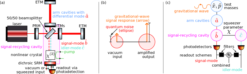
Figure 1: (a) Simplified optical configuration of nondegenerate internal squeezing in a dual-recycled Fabry-Perot Michelson interferometer. Abbreviations are ETM: end test mass, ITM: input test mass, PRM: power-recycling mirror, and SRM: signal-recycling mirror. (b) Representation of how signal-mode readout sensitivity is improved by amplifying the signal more than the noise danilishinQuantumMeasurementTheory2012 . (c) Mode diagram showing that the system consists of three coupled optical modes ($\hat{a},\hat{b},\hat{c}$) and that the gravitational-wave signal indirectly couples into the idler-mode.

In this paper, we explore the technique of nondegenerate internal squeezing explained below. Although this all-optical technique has an equivalent Hamiltonian to stable optomechanical filtering liBroadbandSensitivityImprovement2020 ; bentley_thesis_2021 , it has not been thoroughly examined to date. We analyse its performance in a future gravitational-wave detector with realistic optical loss and demonstrate further sensitivity improvement using variational readout and optimal filtering PhysRevD.65.022002 ; yap2019generation ; PhysRevResearch.3.043079 .

II Concept and model

Nondegenerate internal squeezing consists of a “squeezer” crystal with quadratic polarisability ($\chi^{(2)}$) inside the signal-recycling cavity of a dual-recycled Fabry-Perot Michelson interferometer as shown in Fig. 1(a); the squeezer annihilates a pump photon at (angular) frequency $2\omega_{0}+\Delta$ and creates a pair of photons at “signal-mode” (the carrier frequency $\omega_{0}$) and “idler-mode” ($\omega_{0}+\Delta$ for frequency separation $\Delta\neq 0$) frequencies resonant in the signal-recycling cavity. These pairs are Einstein-Podolsky-Rosen (EPR) correlated, amplified vacuum states schoriNarrowbandFrequencyTunable2002 ; reidDemonstrationEinsteinPodolskyRosenParadox1989 . The signal-mode is coupled to the differential arm mode that contains the gravitational-wave signal bond_2010 ; the idler-mode frequency is not resonant in the arms. This technique improves sensitivity by amplifying the gravitational-wave signal more than the quantum noise, as shown in Fig. 1(b), because the signal comes from the arms but the noise comes primarily from the readout port.

II.1 Analytic model

We model the system using an established analytic Hamiltonian approach danilishinQuantumMeasurementTheory2012 ; miaoEnhancingBandwidthGravitationalWave2015 ; liBroadbandSensitivityImprovement2020 ; korobkoQuantumExpanderGravitationalwave2019 ; schoriNarrowbandFrequencyTunable2002 . A single-mode “coupled-cavity” approximation is valid below the free-spectral range of the arms ($37.5$ kHz miaoEnhancingBandwidthGravitationalWave2015 ) and gives the differential arm mode (with annihilation Heisenberg operator $\hat{a}$), signal-mode ($\hat{b}$), and idler-mode ($\hat{c}$) shown in Fig. 1(c) that evolve according to the Hamiltonian

$$\hat{H} =\hat{H}_{0}+\hat{H}_{\text{int}}+\hat{H}_{\text{mech}}+\hat{H}_{\text{I/O}}$$ (1)

$$\hat{H}_{0}/\hbar =\omega_{0}\hat{a}^{\dagger}\hat{a}+\omega_{0}\hat{b}^{\dagger}\hat{b}+(\omega_{0}+\Delta)\hat{c}^{\dagger}\hat{c}+(2\omega_{0}+\Delta)\hat{u}^{\dagger}\hat{u}$$

$$\hat{H}_{\text{int}} =i\hbar\omega_{s}(\hat{a}\hat{b}^{\dagger}-\hat{a}^{\dagger}\hat{b})+\hbar g(\hat{u}\hat{b}^{\dagger}\hat{c}^{\dagger}+\hat{u}^{\dagger}\hat{b}\hat{c})/2$$

$$\hat{H}_{\text{mech}} =-\alpha(\hat{x}-L_{\text{arm}}h(t))\left(\hat{a}+\hat{a}^{\dagger}\right)/\sqrt{2}+\hat{p}^{2}/(2\mu)$$

$$\frac{\hat{H}_{\text{I/O}}}{i\hbar\sqrt{2}} =\int_{-\infty}^{\infty}\biggl{(}\sqrt{\gamma^{b}_{R}}\hat{B}^{\dagger}(\omega)\hat{b}+\sqrt{\gamma^{c}_{R}}\hat{C}^{\dagger}(\omega)\hat{c}+\sqrt{\gamma_{a}}\hat{N_{a}}^{\dagger}(\omega)\hat{a}$$

$$+\sqrt{\gamma_{b}}\hat{N_{b}}^{\dagger}(\omega)\hat{b}+\sqrt{\gamma_{c}}\hat{N_{c}}^{\dagger}(\omega)\hat{c}+\text{h.c.}\biggr{)}\frac{\text{d}\omega}{\sqrt{2\pi}}\,.$$

Here, $\hat{H}_{0}$ describes the uncoupled harmonic behaviour; $\hat{H}_{\text{int}}$ describes the optical interaction graham1968quantum ; $\hat{H}_{\text{mech}}$ describes the gravitational-wave strain ($h(t)$ for time $t$) coupling through the test masses’ differential mechanical mode (with free mass position $\hat{x}$ and momentum $\hat{p}$) via radiation pressure kimble2001conversion ; and $\hat{H}_{\text{I/O}}$ describes the readout (intra-cavity loss) rate $\gamma^{j}_{R}$ ($\gamma_{j}$) for $j=b,c$ ($a,b,c$) into vacuum bath modes $\hat{B}$,$\hat{C}$ ($\hat{N}_{j}$) that define the incoming fields $\hat{B}^{\text{in}}$,$\hat{C}^{\text{in}}$($\hat{N}^{\text{in}}_{\text{j}}$) gardiner1985input where $\gamma=-c/(4L)\log(1-T)$ for $c$ the speed of light, $L$ the cavity length, and $T$ the readout (loss) port transmission. We omit the natural evolution of the vacuum modes for brevity.

In Eq. 1, $\hbar$ is the reduced Plank constant, $\hat{u}$ is the pump mode, $\omega_{s}\approx c\sqrt{T_{\text{ITM}}/(4L_{\text{arm}}L_{\text{SRC}})}$ is the “sloshing” frequency korobkoQuantumExpanderGravitationalwave2019 ; thuring2007detuned , $T_{\text{ITM}}$ is the input test masses’ transmission, $L_{\text{arm}}$ ($L_{\text{SRC}}$) is the arm (signal-recycling) cavity length, $\chi^{(2)}$ determines the nonlinear coupling rate $g$ paschotta1994nonlinear , $\alpha=\sqrt{2P_{\text{circ}}\omega_{0}\hbar/(cL_{\text{arm}})}$ is the optomechanical coupling rate liBroadbandSensitivityImprovement2020 , $P_{\text{circ}}$ is the circulating (arm) power, and $\mu=M/4$ is the differential mechanical mode’s reduced mass (for test mass mass $M$).

For gravitational-wave detectors, the pump power should be kept below the squeezing threshold and a “reservoir pump” approximation is valid: $\hat{u}\mapsto ue^{i\phi}$ where $u$ is the constant real amplitude and $\phi$ is the pump phase walls_1995 ; martinelli2001classical ; korobkoQuantumExpanderGravitationalwave2019 ; schoriNarrowbandFrequencyTunable2002 . This simplifies the Interaction Frame Heisenberg-Langevin equations-of-motion PhysRevA.31.3761 ; PhysRevA.30.1386 to

$$\dot{\hat{a}} =-\omega_{s}\hat{b}+\frac{i\alpha}{\sqrt{2}\hbar}(\hat{x}-L_{\text{arm}}h(t))-\gamma_{a}\hat{a}+\sqrt{2\gamma_{a}}\hat{N}_{\text{a}}^{\text{in}}$$ (2)

$$\dot{\hat{b}} =\omega_{s}\hat{a}-i\chi e^{i\phi}\hat{c}^{\dagger}-\gamma^{b}_{\text{tot}}\hat{b}+\sqrt{2\gamma^{b}_{R}}\hat{B}^{\text{in}}+\sqrt{2\gamma_{b}}\hat{N}_{\text{b}}^{\text{in}}$$

$$\dot{\hat{c}} =-i\chi e^{i\phi}\hat{b}^{\dagger}-\gamma^{c}_{\text{tot}}\hat{c}+\sqrt{2\gamma^{c}_{R}}\hat{C}^{\text{in}}+\sqrt{2\gamma_{c}}\hat{N}_{\text{c}}^{\text{in}}$$

$$\dot{\hat{x}} =\frac{1}{\mu}\hat{p},\quad\dot{\hat{p}}=\frac{\alpha}{\sqrt{2}}(\hat{a}+\hat{a}^{\dagger})\,.$$

Here, $\chi=gu/2$ is the “squeezer parameter” (to be distinguished from the quadratic polarisability, $\chi^{(2)}$), $\gamma^{j}_{\text{tot}}=\gamma^{j}_{R}+\gamma_{j}$ for $j=b,c$, and each operator (e.g. $\hat{a}$) is implicitly the fluctuating component (e.g. $\delta\hat{a}(t)=\hat{a}(t)-\langle\hat{a}\rangle$ for the time-average $\langle\hat{a}\rangle$). By solving Eq. 2 linearly in the Fourier domain of frequency $\Omega$ to find the cavity modes, using input/output relations at the readout port to find the outgoing modes PhysRevA.31.3761 , and introducing optical detection loss $R_{\text{PD}}\in(0,1)$ and vacuum $\hat{N}_{\text{j,PD}}^{\text{in}}$ for $j=b,c$, the measured quadratures in the Quadrature Picture (e.g. $\hat{X}_{B_{\text{meas}},\theta}=\frac{1}{\sqrt{2}}(e^{-i\theta}\hat{B}_{\text{meas}}+e^{i\theta}\hat{B}_{\text{meas}}^{\dagger})$ for the signal-mode), describing the amplitude and phase of the light at the photodetector, are

$$\vec{\hat{X}}_{\text{meas}} =\mathbf{T}\vec{h}+\sum\nolimits_{j\in\{B/C^{\text{in}},N_{\text{a}}^{\text{in}},N_{\text{b/c}}^{\text{in}},N_{\text{PD}}^{\text{in}}\}}\mathbf{R}_{j}\vec{\hat{X}}_{j}\,.$$ (3)

Here, $\mathbf{T}$ ($\mathbf{R}$) is the resulting signal (noise) transfer matrix describing the relation between an input and the measured output. Each operator-vector contains two quadratures for each of the signal-mode and idler-mode, e.g.

$$\vec{\hat{X}}_{\text{meas}}=(\hat{X}_{B_{\text{meas}},0},\hat{X}_{B_{\text{meas}},\frac{\pi}{2}},\hat{X}_{C_{\text{meas}},0},\hat{X}_{C_{\text{meas}},\frac{\pi}{2}})^{\text{T}},$$ (4)

but $\vec{h}=\tilde{h}(\Omega)(1,1,0,0)^{\text{T}}$ because $\tilde{h}(\Omega)$ is $h(t)$’s Fourier transform and the idler-mode is not resonant in the arms.

Assuming uncorrelated vacuum noise inputs, the measured quantum noise as a (single-sided) power spectral density matrix is $\mathbf{S}_{X}(\Omega)=\sum_{j}\mathbf{R}_{j}({\mathbf{R}_{j}}^{\ast})^{\top}$ danilishinQuantumMeasurementTheory2012 . By Eq. 3, the linear response of the detector to the gravitational wave ($\tilde{h}(\Omega)$) is $\mathbf{T}(1,1,0,0)^{\text{T}}$; since its first component is zero, the fixed–readout angle signal-mode readout measures $\hat{X}_{B_{\text{meas}},\frac{\pi}{2}}$ with sensitivity moore2014gravitational

$$\sqrt{S_{h}(\Omega)}=\sqrt{(\mathbf{S}_{X}(\Omega))_{2,2}}/\absolutevalue{\left(\mathbf{T}(1,1,0,0)^{\text{T}}\right)_{2}}\,.$$ (5)

These results reduce to the expected lossless and high arm loss limits liBroadbandSensitivityImprovement2020 ; graham1968quantum .

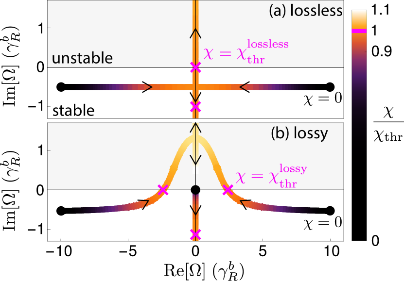
Figure 2: Poles of the transfer functions as the squeezer parameter increases from zero (marked by a dot). Beyond the squeezing threshold (marked by a cross) one or more poles enter the unstable region above the real axis. (a) Lossless and (b) lossy cases using the parameters in Table 1. The $\Omega=0$ pole from the free mass approximation is not shown.

II.2 Stability and squeezing threshold

The dynamical stability and squeezing threshold can be determined from the poles of the transfer functions. Here, the transfer functions (e.g. the coefficients of $\tilde{h}(\Omega)$ and $\hat{X}_{B^{\text{in}},\frac{\pi}{2}}$ in Eq. 3) are rational functions in $\Omega$ with the same denominator for each quadrature and each mode. Moreover, the zeros of the denominator are the same for the signal and noise up to multiplicity and a fixed pole at $\Omega=0$ from the free mass assumption that can be ignored. The system is stable if all of these poles in $\Omega$ have negative imaginary part nise_2019 , which occurs (as shown in Fig. 2) for squeezer parameter below the squeezing threshold given, in the relevant regime $\gamma_{a}<\gamma^{c}_{\text{tot}},\gamma_{a}\ll\omega_{s}$, by

$$\chi_{\text{thr}}^{\text{lossy}}=\sqrt{(\gamma_{a}+\gamma^{b}_{\text{tot}})(\gamma_{a}+\gamma^{c}_{\text{tot}}+\frac{\omega_{s}^{2}}{\gamma^{b}_{\text{tot}}+\gamma^{c}_{\text{tot}}})}\,.$$ (6)

The system — in this model — becomes unstable beyond the squeezing threshold because the reservoir-pump approximation implies unbounded coherent amplification of the cavity modes walls_1995 ; martinelli2001classical ; understanding the system’s physical behaviour above threshold would require extending the model beyond this approximation xingPumpDepletionParametric2022 . This novel method of determining threshold recovers the known values in the lossless ($\chi_{\text{thr}}^{\text{lossless}}=\omega_{s}$ liBroadbandSensitivityImprovement2020 ) and high arm loss ($\sqrt{\gamma^{b}_{\text{tot}}\gamma^{c}_{\text{tot}}}$ graham1968quantum ) limits.

III Results

carrier wavelength, $2\pi c/\omega_{0}$	2 $\mu\text{m}$
arm cavity length, $L_{\text{arm}}$	4 km
circulating arm power, $P_{\text{circ}}$	3 MW
test mass mass, $M$	200 kg
injected external squeezing	10 dB
intra-cavity loss, $T_{l,a;b(c)}$	100 ; 1000 (1000) ppm
detection loss, $R_{\text{PD}}$	$10\%$
SRM transmission, $T_{\text{SRM},b(c)}$	0.0152 (0)	0.046 (0)
SRC length, $L_{\text{SRC}}$	366.5 m	56 m
ITM transmission, $T_{\text{ITM}}$	0.0643	0.002
sloshing frequency, $\omega_{s}$	5 kHz	2.256 kHz
readout rate, $\gamma^{b(c)}_{R}$	0.5 (0) kHz	10.038 (0) kHz

Table 1: Baseline parameters for signal-mode readout with deviations shown in boldface next to the corresponding LIGO Voyager values LIGO_Voyager . The idler-mode values are shown in parentheses next to the corresponding signal-mode values and are achievable by means of a dichroic if the frequency separation ($\Delta$) can be made sufficiently large, e.g., using additional cavities. Although 10 dB frequency-dependent external squeezing is injected into the signal-mode (and, later, idler-mode), only ${\sim}7$ dB is measured due to loss.

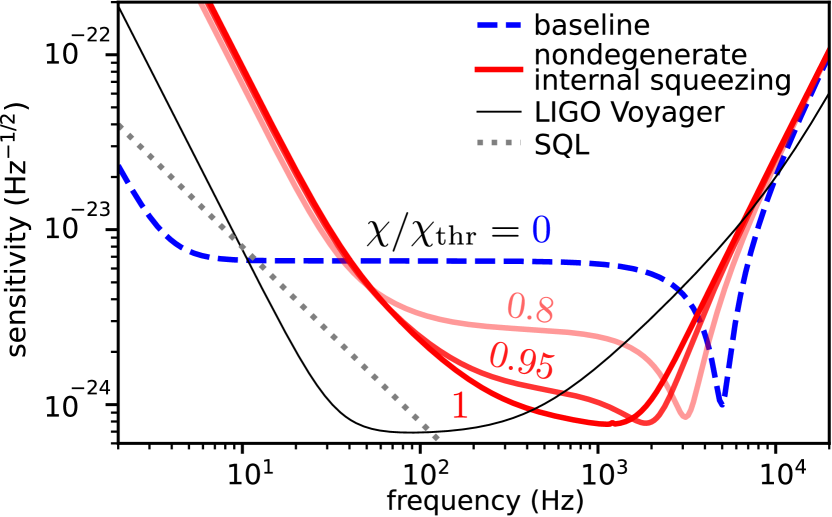
Figure 3: Sensitivity versus frequency for signal-mode readout with different squeezer parameters. The $\omega_{s}=5$ kHz feature in the baseline curve is the coupled-cavity pole. The baseline curve exceeds the Standard Quantum Limit (SQL) danilishinQuantumMeasurementTheory2012 using frequency-dependent external squeezing which is compatible and used with internal squeezing. The parameters in Table 1 are used. The LIGO Voyager LIGO_Voyager quantum noise–limited design curve is also shown.

Nondegenerate internal squeezing improves sensitivity at 40 Hz–4 kHz at the expense of frequencies below 40 Hz as shown in Fig. 3. Increasing the squeezer parameter further improves sensitivity without sacrificing bandwidth or requiring increased circulating power or arm length. These results use the parameters and realistic optical loss zhangBroadbandSignalRecycling2021 ; Danilishin_2019 in Table 1 based on LIGO Voyager LIGO_Voyager ; Table 1 contains a longer signal-recycling cavity than LIGO Voyager to improve kilohertz sensitivity liBroadbandSensitivityImprovement2020 .

Given current estimates of the neutron-star equation-of-state, the sensitivity required to detect a typical binary neutron-star post-merger signal at $50$ Mpc is $\sqrt{S_{h}}=5\times 10^{-25}\mathrm{Hz}^{-1/2}$ from 1–4 kHz PhysRevD.100.104029 ; miaoDesignGravitationalWaveDetectors2018 . With $\chi/\chi_{\text{thr}}=0.986$ and the parameters in Table 1 except $T_{\text{SRM},c}=110$ ppm (meaning that technological progress is required), signal-mode readout can achieve this target at ${\sim}1$ kHz. Achieving it across the entire 1–4 kHz band would require reduced loss and increased circulating power, arm length, pump power, and/or injected external squeezing.

III.1 Tolerance to decoherence from optical loss

Nondegenerate internal squeezing is more tolerant to decoherence from optical detection loss than a conventional gravitational-wave detector as shown in Fig. 4. Loss decreases the signal and pulls the quantum noise towards the vacuum level. When amplified, however, the signal and noise decrease at approximately the same rate and the sensitivity remains approximately constant. In comparison, degenerate internal squeezing experiences worse sensitivity degradation because the squeezed noise increases towards the vacuum level korobkoQuantumExpanderGravitationalwave2019 ; adyaQuantumEnhancedKHz2020 ; korobkoCompensatingQuantumDecoherenceTalk2021 .

Realistically, signal-mode readout is limited by idler-mode loss which agrees with mechanical idler-mode loss limiting stable optomechanical filtering liBroadbandSensitivityImprovement2020 ; miao2019quantum . To match the sensitivity of stable optomechanical filtering from Ref. liBroadbandSensitivityImprovement2020 , which assumes that the mechanical loss parameter-of-interest is a factor of ${\sim}16$ below existing technology, this technique requires a factor of ${\sim}18$ reduction in optical idler-mode loss; the required environmental temperature divided by mechanical quality factor (optical loss) is $6\times 10^{-10}K$ miaoEnhancingBandwidthGravitationalWave2015 (110 ppm) compared to $9.7\times 10^{-9}K$ masonetal2019 ; pageEnhancedDetectionHigh2018 (2000 ppm barsottiLIGOdoc2016 ) currently possible. This suggests that this technique is a viable all-optical alternative to stable optomechanical filtering. This is a key result: this loss-resistant technique is comparable to existing proposals.

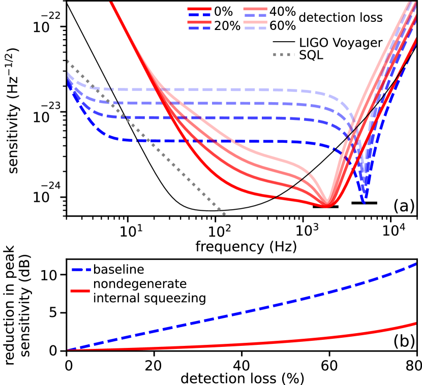
Figure 4: (a) Sensitivity versus frequency for signal-mode readout with different optical detection loss. (b) Peak sensitivity versus detection loss normalised to the peak sensitivity with $0\%$ detection loss — higher values indicate greater sensitivity degradation. The parameters, including intra-cavity loss, in Table 1 are used with $\chi/\chi_{\text{thr}}=0.95$.

III.2 Alternative readout schemes

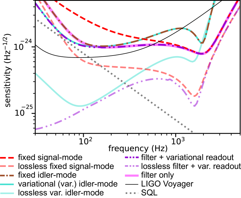
Figure 5: Sensitivity versus frequency for alternative readout schemes. The parameters in Table 1 are used with $\chi/\chi_{\text{thr}}=0.95$ except $T_{\text{SRM},c}\approx 1.54\times 10^{-4}$.

Idler-mode readout is possible, e.g. by an additional homodyne readout at the idler-mode frequency to measure $\hat{X}_{C_{\text{meas}},\theta_{c}}$, because the gravitational-wave signal is coupled in via the squeezer as shown in Fig. 1(c). Since the idler-mode is not directly coupled to the arms, fixed ($\theta_{c}=\phi$) idler-mode readout improves sensitivity differently than signal-mode readout as shown in Fig. 5. One advantage of idler-mode readout is that the idler-mode wavelength can be chosen to match higher quantum efficiency photodetectors than the $2~{}\mu\text{m}$ wavelength signal-mode singh_2019 . Realistically, idler-mode readout is limited by signal-mode loss ($T_{l,b}$), however, using idler-mode readout alone with the signal-mode readout port closed does not outperform a signal-mode readout detector.

Variational readout of each mode, achieved via homodyne readout and a filter cavity PhysRevD.65.022002 , can measure $\hat{X}_{C_{\text{vary}}}=\hat{X}_{C_{\text{meas}},\theta_{c}(\Omega)}$ and $\hat{X}_{B_{\text{vary}}}$ similar. This improves idler-mode readout, as shown in Fig. 5, by reducing the amplified quantum radiation-pressure noise danilishinQuantumMeasurementTheory2012 ; hild2012beyond using correlations generated ponderomotively at the test masses and coupled from the signal-mode PhysRevD.65.022002 . The correlation of the signal-mode quadratures is too low to improve sensitivity for high $\chi/\chi_{\text{thr}}$ (e.g. $0.95$).

The optimal readout scheme measures the optimal coherent linear combination of the signal-mode and idler-mode, as shown in Fig. 1(c), at each frequency, i.e. $\hat{X}_{\text{opt}}=\sum_{i\in\{B,C\}}G_{i}(\Omega)\hat{X}_{i_{\text{vary}}}\,,$ where $G_{i}$ are complex, acausal “filter” coefficients, such that $\absolutevalue{G_{B}}^{2}+\absolutevalue{G_{C}}^{2}=1$, simultaneously numerically optimised with the readout angles ($\theta_{b},\theta_{c}$). This scheme (“filter + variational readout” in Fig. 5) further improves sensitivity via recovering squeezing from the EPR-correlation ma_2017 ; schoriNarrowbandFrequencyTunable2002 ; liEnhancingInterferometerSensitivity2021 . Although decoherence reduces the EPR-correlation, the optimal filter remains more tolerant to detection loss than a conventional detector. In the lossless (i.e. no detection or intra-cavity loss) limit, the amplified quantum radiation-pressure noise at 30 Hz can be reduced by up to two orders-of-magnitude as shown in Fig. 5. Realistically, however, the filter is limited by signal-mode and idler-mode loss, and the optimal filter without variational readout (“filter only” in Fig. 5) achieves the same sensitivity above ${\sim}200$ Hz and is more feasible for a broadband (100 Hz–4 kHz) future gravitational-wave detector.

IV Conclusions

In this paper, we have explored nondegenerate internal squeezing: a viable, all-optical technique to enhance sensitivity. Using an analytic Hamiltonian model, we have found it to (1) be stable, (2) realistically improve sensitivity without sacrificing bandwidth or increasing the circulating power or arm length, and (3) be tolerant to decoherence from optical detection loss — an advantage over existing proposals. Using the parameters of a modified LIGO Voyager, we have shown that optimal filtering without variational readout is this technique’s preferred readout scheme out of those considered for kilohertz (1–4 kHz) and broadband (100 Hz–4 kHz) gravitational-wave detection. How to thermally compensate the 100 kW of power incident on the beamsplitter and achieve the large frequency separation required in Table 1 need further analysis. This technique may be used in general cavity-based quantum metrology, and our model characterises equivalent Hamiltonian systems, e.g. enhanced microwave axion detectors liBroadbandSensitivityImprovement2020 ; MARSH20161 ; PhysRevX.9.021023 .

- (1) B. P. Abbott, R. Abbott, T. Abbott, S. Abraham, F. Acernese, K. Ackley, C. Adams, V. Adya, C. Affeldt, M. Agathos, et al. 2020. Living Rev. Relativ., 23(1):1–69.
- (2) J. Aasi, B. P. Abbott, R. Abbott, T. Abbott, M. R. Abernathy, K. Ackley, C. Adams, T. Adams, P. Addesso, and et al. 2015. Class. Quantum Grav., 32:074001.
- (3) F. Acernese, M. Agathos, K. Agatsuma, D. Aisa, N. Allemandou, A. Allocca, J. Amarni, P. Astone, G. Balestri, G. Ballardin, et al. 2014. Class. Quantum Grav., 32(2):024001.
- (4) T. Akutsu, M. Ando, K. Arai, Y. Arai, S. Araki, A. Araya, N. Aritomi, H. Asada, Y. Aso, S. Atsuta, et al. 2018. arXiv:1811.08079.
- (5) R.-G. Cai, Z. Cao, Z.-K. Guo, S.-J. Wang, and T. Yang. 2017. Natl. Sci. Rev., 4(5):687–706.
- (6) M. Maggiore. Gravitational Waves: Volume 1: Theory and Experiments. Oxford University Press, 2007.
- (7) B. P. Abbott, R. Abbott, T. D. Abbott, S. Abraham, F. Acernese, K. Ackley, C. Adams, R. X. Adhikari, V. B. Adya, C. Affeldt, et al. 2019. Phys. Rev. X, 9(3):031040.
- (8) R. Abbott, T. D. Abbott, S. Abraham, F. Acernese, K. Ackley, A. Adams, C. Adams, R. X. Adhikari, V. B. Adya, C. Affeldt, et al. 2021. Phys. Rev. X, 11:021053.
- (9) R. Abbott, T. D. Abbott, F. Acernese, K. Ackley, C. Adams, N. Adhikari, R. X. Adhikari, V. B. Adya, C. Affeldt, D. Agarwal, et al. 2021. arXiv:2111.03606 [gr-qc].
- (10) S. Vitale. 2021. Science, 372(6546):eabc7397.
- (11) M. Breschi, S. Bernuzzi, F. Zappa, M. Agathos, A. Perego, D. Radice, and A. Nagar. 2019. Phys. Rev. D, 100:104029.
- (12) H. Miao, H. Yang, and D. Martynov. 2018. Phys. Rev. D, 98(4):044044.
- (13) R. X. Adhikari, K. Arai, A. F. Brooks, C. Wipf, O. Aguiar, P. Altin, B. Barr, L. Barsotti, R. Bassiri, A. Bell, et al. 2020. Class. Quantum Grav., 37(16):165003.
- (14) K. Ackley, V. B. Adya, P. Agrawal, P. Altin, G. Ashton, M. Bailes, E. Baltinas, A. Barbuio, D. Beniwal, C. Blair, et al. 2020. Publ. Astron. Soc, 37.
- (15) D. Reitze, R. X. Adhikari, S. Ballmer, B. Barish, L. Barsotti, G. Billingsley, D. A. Brown, Y. Chen, D. Coyne, R. Eisenstein, et al. 2019. arXiv:1907.04833.
- (16) M. Maggiore, C. Van Den Broeck, N. Bartolo, E. Belgacem, D. Bertacca, M. A. Bizouard, M. Branchesi, S. Clesse, S. Foffa, J. García-Bellido, et al. 2020. J. Cosmol. Astropart., 2020(03):050.
- (17) M. Shibata, K. Kyutoku, T. Yamamoto, and K. Taniguchi. 2009. Phys. Rev. D, 79:044030.
- (18) C. D. Ott. 2009. Class. Quantum Grav., 26(6):063001.
- (19) C. Messenger, K. Takami, S. Gossan, L. Rezzolla, and B. S. Sathyaprakash. 2014. Phys. Rev. X, 4:041004.
- (20) A. Buikema, C. Cahillane, G. L. Mansell, C. D. Blair, R. Abbott, C. Adams, R. X. Adhikari, A. Ananyeva, S. Appert, K. Arai, et al. 2020. Phys. Rev. D, 102(6):062003.
- (21) C. M. Caves. 1981. Phys. Rev. D, 23:1693–1708.
- (22) J. Mizuno. PhD thesis, AEI-Hannover, MPI for Gravitational Physics, Max Planck Society, 1995.
- (23) H. Miao, R. X. Adhikari, Y. Ma, B. Pang, and Y. Chen. 2017. Phys. Rev. Lett., 119(5):050801.
- (24) A. F. Brooks, G. Vajente, H. Yamamoto, R. Abbott, C. Adams, R. X. Adhikari, A. Ananyeva, S. Appert, K. Arai, J. S. Areeda, et al. 2021. Appl. Opt., 60(13):4047.
- (25) M. Evans, S. Gras, P. Fritschel, J. Miller, L. Barsotti, D. Martynov, A. Brooks, D. Coyne, R. Abbott, R. X. Adhikari, et al. 2015. Phys. Rev. Lett., 114:161102.
- (26) L. Barsotti, J. Harms, and R. Schnabel. 2018. Rep. Prog. Phys., 82(1):016905.
- (27) M. Tse, H. Yu, N. Kijbunchoo, A. Fernandez-Galiana, P. Dupej, L. Barsotti, C. D. Blair, D. D. Brown, S. E. Dwyer, A. Effler, et al. 2019. Phys. Rev. Lett., 123(23):231107.
- (28) J. Aasi, J. Abadie, B. P. Abbott, R. Abbott, T. D. Abbott, M. R. Abernathy, C. Adams, T. Adams, P. Addesso, R. X. Adhikari, et al. 2013. Nat. Photonics, 7(8):613–619.
- (29) D. Ganapathy, L. McCuller, J. G. Rollins, E. D. Hall, L. Barsotti, and M. Evans. 2021. Phys. Rev. D, 103(2).
- (30) F. Acernese, M. Agathos, L. Aiello, A. Allocca, A. Amato, S. Ansoldi, S. Antier, M. Arène, N. Arnaud, S. Ascenzi, et al. 2019. Phys. Rev. Lett., 123:231108.
- (31) K. L. D. and. 2015. Journal of Physics: Conference Series, 610:012015.
- (32) M. Page, J. Qin, J. La Fontaine, C. Zhao, and D. Blair. 2018. Phys. Rev. D, 97(12):124060.
- (33) M. Korobko, Y. Ma, Y. Chen, and R. Schnabel. 2019. Light Sci. Appl., 8(1):118.
- (34) V. B. Adya, M. J. Yap, D. Töyrä, T. G. McRae, P. A. Altin, L. K. Sarre, M. Meijerink, N. Kijbunchoo, B. J. J. Slagmolen, R. L. Ward, et al. 2020. Class. Quantum Grav., 37(7):07LT02.
- (35) X. Li, M. Goryachev, Y. Ma, M. E. Tobar, C. Zhao, R. X. Adhikari, and Y. Chen. 2020. arXiv:2012.00836 [quant-ph].
- (36) X. Li, J. Smetana, A. S. Ubhi, J. Bentley, Y. Chen, Y. Ma, H. Miao, and D. Martynov. 2021. Phys. Rev. D, 103:122001.
- (37) H. Miao, Y. Ma, C. Zhao, and Y. Chen. 2015. Phys. Rev. Lett., 115(21):211104.
- (38) A. Wicht, K. Danzmann, M. Fleischhauer, M. Scully, G. Müller, and R.-H. Rinkleff. 1997. Opt. Commun., 134(1):431–439.
- (39) M. Ying, X. Chen, Y. Hsu, D. Tsai, H. Pan, S. Chao, A. Sunderland, M. Page, B. Neil, L. Ju, et al. 2021. J. Phys., 54(3).
- (40) S. L. Danilishin and F. Y. Khalili. 2012. Living Rev. Relativ., 15(1):5.
- (41) J. Bentley. PhD thesis, University of Birmingham, 2021.
- (42) H. J. Kimble, Y. Levin, A. B. Matsko, K. S. Thorne, and S. P. Vyatchanin. 2001. Phys. Rev. D, 65:022002.
- (43) M. J. Yap, P. Altin, T. G. McRae, R. L. Ward, B. J. J. Slagmolen, and D. E. McClelland. 2020. Nat. Photonics, 14:223–226.
- (44) D. W. Gould, M. J. Yap, V. B. Adya, B. J. J. Slagmolen, R. L. Ward, and D. E. McClelland. 2021. Phys. Rev. Res., 3:043079.
- (45) C. Schori, J. L. Sørensen, and E. S. Polzik. 2002. Phys. Rev. A, 66(3):033802.
- (46) M. D. Reid. 1989. Phys. Rev. A, 40(2):913–923.
- (47) A. Freise and K. Strain. 2010. Living Rev. Relativ., 13(1).
- (48) R. Graham and H. Haken. 1968. Z. Phys. A, 210(3):276–302.
- (49) H. J. Kimble, Y. Levin, A. B. Matsko, K. S. Thorne, and S. P. Vyatchanin. 2001. Phys. Rev. D, 65(2):022002.
- (50) C. W. Gardiner and M. J. Collett. 1985. Phys. Rev. A, 31(6):3761.
- (51) A. Thüring, R. Schnabel, H. Lueck, and K. Danzmann. 2007. Optics letters, 32(8):985–987.
- (52) R. Paschotta, K. Fiedler, P. Kürz, and J. Mlynek. 1994. Appl. Phys. B, 58(2):117–122.
- (53) D. F. Walls and G. Milburn. Quantum Optics. Springer-Verlag, 1995.
- (54) M. Martinelli, C. Garrido Alzar, P. Souto Ribeiro, and P. Nussenzveig. 2001. Braz. J. Phys., 31:597–615.
- (55) C. W. Gardiner and M. J. Collett. 1985. Phys. Rev. A, 31:3761–3774.
- (56) M. J. Collett and C. W. Gardiner. 1984. Phys. Rev. A, 30:1386–1391.
- (57) C. J. Moore, R. H. Cole, and C. P. Berry. 2014. Class. Quantum Grav., 32(1):015014.
- (58) N. S. Nise. Control Systems Engineering. Wiley, 8th edition, 2019.
- (59) W. Xing and T. C. Ralph. 2022. arXiv:2201.01372 [quant-ph].
- (60) T. Zhang, J. Bentley, and H. Miao. 2021. Galaxies, 9(1):3.
- (61) S. L. Danilishin, F. Y. Khalili, and H. Miao. 2019. Living Rev. Relativ., 22(1).
- (62) M. Korobko, S. Steinlechner, J. Südbeck, and R. Schnabel. 2021. LIGO-Virgo-KAGRA Collaboration Meeting on September 6th. LIGO Doc. G2101870-v1.
- (63) H. Miao, N. D. Smith, and M. Evans. 2019. Phys. Rev. X, 9(1):011053.
- (64) D. Mason, J. Chen, M. Rossi, Y. Tsaturyan, and A. Schliesser. 2019. Nat. Phys., 15(8):745–749.
- (65) L. Barsotti. 2016. LIGO Doc. G1601199-v2.
- (66) S. Singh. 2019. LIGO Doc. T1900380-v1.
- (67) S. Hild. 2012. Class. Quantum Grav., 29(12):124006.
- (68) Y. Ma, H. Miao, B. Pang, M. Evans, C. Zhao, J. Harms, R. Schnabel, and Y. Chen. 2017. Nat. Phys., 13(8):776–780.
- (69) D. J. Marsh. 2016. Phys. Rep., 643:1–79.
- (70) M. Malnou, D. A. Palken, B. M. Brubaker, L. R. Vale, G. C. Hilton, and K. W. Lehnert. 2019. Phys. Rev. X, 9:021023.
- (71) Wolfram Research, Inc. 2010.
- (72) G. Van Rossum and F. L. Drake Jr. Python Tutorial. Centrum voor Wiskunde en Informatica Amsterdam, The Netherlands, 1995.
- (73) F. Pérez and B. E. Granger. 2007. Comput. Sci. Eng., 9(3).
- (74) T. Kluyver, B. Ragan-Kelley, F. Pérez, B. Granger, M. Bussonnier, J. Frederic, K. Kelley, J. Hamrick, J. Grout, S. Corlay, et al. In Positioning and Power in Academic Publishing: Players, Agents and Agendas, pages 87–90, 2016.
- (75) T. E. Oliphant. A guide to NumPy. Trelgol Publishing USA, 2006.
- (76) J. D. Hunter. 2007. Comput. Sci. Eng., 9(3):90–95.
- (77) A. Franzen. 2009. http://www.gwoptics.org/ComponentLibrary/.