Overparametrized linear dimensionality reductions:
From projection pursuit to two-layer neural networks111An earlier version of this paper was accepted for presentation at the Conference on Learning Theory (COLT) 2022, with the title “High-Dimensional Projection Pursuit:
Outer Bounds and Applications to Interpolation in Neural Networks.”
Abstract
Given a cloud of data points in , consider all projections onto -dimensional subspaces of and, for each such projection, the empirical distribution of the projected points. What does this collection of probability distributions look like when grow large?
We consider this question under the null model in which the points are i.i.d. standard Gaussian vectors, focusing on the asymptotic regime in which , with , while is fixed. Denoting by the set of probability distributions in that arise as low-dimensional projections in this limit, we establish new inner and outer bounds on . In particular, we characterize the Wasserstein radius of up to logarithmic factors, and determine it exactly for . We also prove sharp bounds in terms of Kullback-Leibler divergence and Rényi information dimension.
The previous question has application to unsupervised learning methods, such as projection pursuit and independent component analysis. We introduce a version of the same problem that is relevant for supervised learning, and prove a sharp Wasserstein radius bound. As an application, we establish an upper bound on the interpolation threshold of two-layers neural networks with hidden neurons.
1 Introduction and main results
1.1 A null model for unsupervised learning
Given data points , Friedman and Tukey [FT74] proposed to look for interesting structures by plotting histograms of their projections onto -dimensional subspaces (with ). They suggested to seek for projections that maximize a certain index of clustering of the resulting histograms. Diaconis and Freedman [DF84] showed that under incoherence conditions on the points , most one-dimensional projections are nearly Gaussian. They also studied the null model in which , in the high-dimensional setting . They proved that, if then the ‘least Gaussian’ one-dimensional projection converges to a standard Gaussian (in Kolmogorov-Smirnov distance), while, if , it does not.
We will study the (Gaussian) null model of [DF84], under the proportional asymptotics . Let denote the space of all probability measures on , and . Denote by the matrix with rows , . We say that is -feasible if there exists a sequence of random orthogonal matrices () such that the empirical distribution of the projections converges weakly to , in probability with respect to the randomness in . (Here denotes additional randomness that can be used in the construction of .) In formulas:
| (1) | ||||
| (2) |
(See Section 2 for clarifications about this definition.)
Understanding is relevant for a broad array of unsupervised learning methods. Indeed, non-Gaussian projections are sought by independent component analysis [HO00], blind deconvolution [LWDF11], and related methods [BKS+06, SNS16, Lop18].
The problem of characterizing was recently studied by Bickel, Kur and Nadler [BKN18], for the case . Denoting by the second moment of , and by the Kolmogorov-Smirnov distance between and , [BKN18] proved the following:
| (3) | ||||
| (4) |
The paper [BKN18] also proved that certain mixtures of a Gaussian and a non-Gaussian component are feasible for , leading the authors to conjecture that this is the case for all the feasible distributions.
We will establish several new results on this model:
- Wasserstein radius for .
-
Denoting by the second Wasserstein distance between two probability measures and , we prove that . Note that this implies as a corollary the outer bound in Eq. (3), but it is significantly stronger.
- KL-Wasserstein outer bound.
-
We show that, for any , is contained in a neighborhood of the set of distributions such that , with the Kullback-Leibler (KL) divergence (relative entropy). As a corollary, this bound implies an upper bound on the radius of that is tight within a factor . However, the KL bound is significantly tighter than the bound for distributions that are less regular than Gaussians.
- Information dimension bound.
-
Denoting by the lower information dimension of (see Definition 2.1), we prove that is contained in for .
For instance, if is supported on an -dimensional smooth manifold in , then , and therefore is -feasible only if .
- -KL divergence inner bound.
-
We establish an inner bound for the feasibility set , which is expressed in terms of and KL divergence. For probability distributions for which these two distances from are comparable, this inner bound implies a lower bound on the maximum for which is feasible, which is tight up to a logarithmic factor. As a comparison, the inner bound result in Eq. (3) only applies to the case .
1.2 A null model for supervised learning
Our main motivation to revisit projection pursuit comes from supervised learning, and we establish their connection below.
To be definite, we consider a data model whereby are i.i.d., with isotropic Gaussian covariates and responses depending on low-dimensional projections of the ’s. Namely, for , let be an orthogonal matrix such that . We assume that the conditional distribution of given only depends on :
| (5) |
(and ) for a measurable function . We notice in passing that this model can be easily generalized to continuous sub-Gaussian responses , and our proofs apply to this case as well.
In many supervised learning methods, one seeks a model that only depends on a low-dimensional projection of the covariates. Fitting such a model requires to consider the possible distributions over that can be obtained by projecting the covariates onto an -dimensional subspace of .
This motivates the following definition. We say that is -feasible if there exists a sequence of random orthogonal matrices () such that the empirical distribution of the pairs converges weakly to (in probability with respect to the randomness in , and ). In formulas:
Characterizing the set gives access to a number of statistical quantities of interest. In this paper, we present the following results.
- General ERM asymptotics.
-
We consider a class of empirical risk minimization (ERM) problems over functions of the form , where both and are optimized over. We show that the asymptotics of the minimum empirical risk can be expressed in terms of a variational problem over the feasibility set .
- Wasserstein bound for .
-
We prove an outer bound on for general , which generalizes the Wasserstein radius result obtained in the unsupervised setting. In fact this outer bound characterizes the maximum distance between the empirical distribution of one-dimensional projections and the expected distribution.
- Interpolation for two-layer networks.
-
As a corollary to the previous result, we prove that a neural network with two-layers and hidden neurons can separate data points in dimensions with margin only if (where the limit with is understood). Earlier bounds only required .
- Margin distributions for linear classifier.
-
We demonstrate the tightness of our bound by deriving the asymptotic distribution of the margins in linear max-margin classification.
The rest of this paper is organized as follows. We formally state our results for unsupervised and supervised learning, respectively, in Section 2, Section 3, and Section 4. We describe some of the proof ideas in Section 5, with actual proofs deferred to the appendices.
Notations
We denote by the Dirac measure at , where is a measurable space. The set of all probability measures on is denoted as . For a random variable , denotes the probability distribution of . For a positive integer , we let be the set . For two measures and , we use to denote their product measure.
We consistently use lowercase letters to denote scalars, boldface lowercase letters to denote vectors, and boldface uppercase letters to denote matrices. For a scalar , we write and . For two vectors and , denotes their scalar product. We use to denote the Euclidean norm of a vector . We denote by the unit sphere in .
We always use and to denote the CDF and PDF of a standard normal variable, respectively. We write if and are two independent random variables. We denote by the set of all orthogonal matrices such that .
Finally, whenever clear from the context, we identify a vector with its transpose : This reduces some notational burden, and amounts to identifying with its dual.
2 Outer bounds: Unsupervised learning
Before stating our results, it is useful to recall the definition of feasibility set (2), and to clarify one element of this definition. Note that is a random probability distribution on . We say that in probability if, for any , , where is a distance that metrizes weak convergence. For instance can be taken to be the bounded Lipschitz distance or the Lévy-Prokhorov metric.
Given two probability distributions on , we denote by the second Wasserstein distance between and . Namely
| (6) |
where the infimum is taken over the space of couplings of .
Theorem 2.1 (Wasserstein radius for ).
Consider the case . Then for any , we have
| (7) |
Remark 2.1.
The supremum above is achieved by taking . Indeed, as shown in the proof of Theorem 2.1, this distribution is feasible by taking , where is the top right singular vector of .
Recall the definition of the KL divergence. Given two probability measures and on a measure space , if is absolutely continuous with respect to , then
| (8) |
where denotes the Radon-Nikodym derivative of with respect to . Otherwise, .
Theorem 2.2 (KL-Wasserstein outer bound).
For , define the following neighborhood of :
Then, there exist absolute constants and such that for any , we have
As a direct consequence of Theorem 2.2, we obtain the following:
Theorem 2.3.
There exists an absolute constant such that
Further, there exists such that .
Remark 2.2.
This theorem gives an upper bound on the radius of for all . A comparison with Theorem 2.1 suggests that the factor might be due to the artifact of the proof, and we expect it to be removed via a more refined analysis. On the other hand, the lower bound shows that the factor is necessary.
Let us emphasize that even in the one-dimensional case, Theorem 2.2 is not a consequence of Theorem 2.1. There exist infeasible distributions that are excluded by Theorem 2.2 and satisfy . An interesting case is the one in which is supported on a set of lower dimension. In particular for certain values of , probability measures supported on low-dimensional manifolds in are not feasible, no matter how close they are to the standard normal distribution in distance.
Definition 2.1 (Information dimension [Rén59]).
Let be an arbitrary random variable in , and denote for the following discretization of :
Let denote the Shannon entropy of a discrete random variable , i.e., , and define
where and are called lower and upper information dimensions of , respectively. With an abuse of notation, we will write , when .
Theorem 2.4.
Assume , and satisfies . Then, is not -feasible. As a consequence, if is supported on an -dimensional smooth manifold in (where ) such that , then is not -feasible.
Remark 2.3.
Since any discrete distribution with finite entropy has information dimension equal to , we know that is not -feasible provided . As a consequence, for any , , we can construct a distribution such that , and yet is infeasible. This is achieved by discretizing on a scale , obtaining that is a countable combination of point masses at points in .
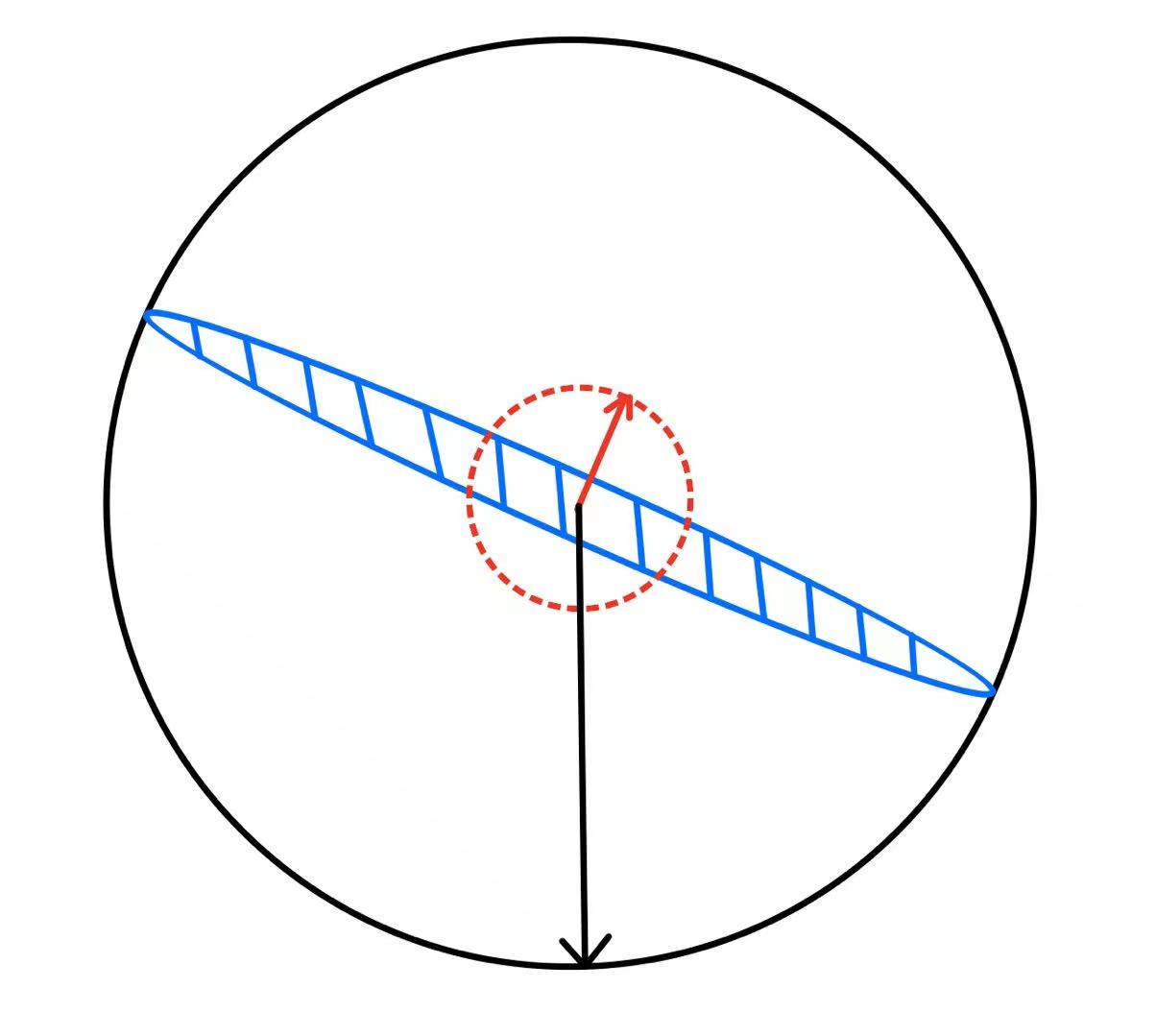
A cartoon of the geometry of is given in Figure 1.
Note that, since is closed under weak convergence (Lemma E.7), the last infeasibility result applies to distributions that have a density in but are sufficiently close —say— to a low-dimensional manifold.
3 Inner bounds: Unsupervised learning
In this section, we present our main results on inner bounds for the feasibility set . Given a target distribution , we will show that it is feasible (below a critical value of ) in two steps: First, we consider a discretization of supported on a finite set of points . We will prove that the corresponding discretization of the empirical distribution of the projected points converges to the discretization of . We then establish feasibility of by taking increasingly denser meshes .
For and a finite set , define the -discretization of as follows:
Definition 3.1 (-discretization).
For , denote the projection of onto as , namely
The -discretization of is then defined as where .
Let be a probability distribution with support on such that for every . We next define the feasibility lower bound for . As stated formally below, for we can find projections such that the -discretization of the empirical distribution of projected points is close to with probability bounded away from zero.
Definition 3.2 (Feasibility threshold of ).
For satisfying , let be the following probability distribution supported on :
We define the probability distribution supported on via:
| (9) |
where, specializing Eq. (8), we have . In words, is the information projection of the distribution onto the set of distributions on whose both margins are .
Next define via
| (10) |
(We set if , which is equivalent to defining only when .)
Finally, we define
| (11) |
We next establish that is indeed a lower bound on the feasibility threshold for . (Here, feasibility is understood for the discretized projections.)
Theorem 3.1.
Let be a probability distribution on the finite set giving strictly positive mass to every . If , then there exists a constant and a sequence of a random orthogonal matrices such that
where is the empirical distribution of the projected data points, and is the total variation distance.
In the next two subsections, we will apply this result to prove lower bounds on the supremum of such that for a probability distribution with a density on . We treat the cases and separately and carry out a more accurate analysis in the first case. As anticipated above, our proof is based on approximating by for a sequence of finite sets of increasing cardinality. It will be crucial to control the lower bounds along such a sequence. The following variational representation of the KL divergence turns out to be particularly useful.
Lemma 3.2 (Donsker-Varadhan representation of KL divergence).
Let and be two probability measures on the same space , then we have
Moreover, recalling and from Definition 3.2, and denoting
we get that
3.1 Inner bound for
Here we specialize our results to the case , and consequently obtain an inner bound for . To simplify our treatment, we will require that our target distribution has a density on , which satisfies the following assumption:
Assumption 3.1.
Denote by the density of the standard normal distribution. Assume that , , and that the chi-square distance between and is finite, namely
Since the KL divergence is always dominated by the chi-square distance, we know that .
Theorem 3.3 (Lower bound on feasibility threshold for ).
Let have density function satisfying Assumption 3.1, and denote
(Note that by Cauchy-Schwarz inequality.)
Define the following lower bound on the feasibility threshold for :
| (12) |
where . Then, as long as , is -feasible.
Proposition 3.4 (Characterization of ).
Let be as defined in Eq. (12). Then, we have
Remark 3.1.
Recall that always holds. If, in addition, , for a constant , then there exists another constant depending on such that the following lower bound on the feasibility threshold holds:
This matches the outer bound in Theorem 2.2 up to a logarithmic factor.
3.2 Inner bound for general
We now generalize the results in Section 3.1 to dimensions .
Assumption 3.2.
We assume that has zero mean, and . In particular, has a density which we denote by . Let be the density of , and further denote . For any , the function has the following multivariate Hermite expansion (see the proof of Theorem 3.5):
where , , , and . Moreover, we know that for ,
which is independent of due to rotational invariance of .
Theorem 3.5 (Lower bound on feasibility threshold for ).
Let satisfy Assumption 3.2, and define to be the supremum of all such that the following happens: There exists a neighborhood of , such that for any having singular values ,
and that
Then, as long as , is -feasible.
4 Main results: Supervised learning
In order to motivate our generalization of previous results to supervised learning, consider the following empirical risk minimization (ERM) problem:
| (13) |
Here the minimization is over in , the set of orthogonal matrices, and in a set of functions . For instance, we could consider (the set of functions with Lipschitz modulus at most ), or so that is a two-layer neural network with total second-layer weights bounded by and orthonormal first-layer weights. Finally allows to treat all two-layer networks with neurons and bounded first and second-layer weights.
The next proposition establishes that the minimum of the empirical risk is given asymptotically by a variational problem over the feasibility set .
Proposition 4.1.
Assume with . Further assume to be bounded continuous, and , for some constant . Then, we have
| (14) |
(For a sequence of random variables and a constant , if is the infimum of all such that .)
4.1 Wasserstein outer bound for
Throughout this section, we assume , so that . Recall the data model defined in Section 1.2, whereby and are such that
with . Notice that we allow for .
We are interested in the empirical distribution of , denoted by
We begin with an elementary calculation that characterizes the asymptotics of this distribution for a vector that does not depend on the data .
Lemma 4.2.
Let the random variables be such that
| (15) |
For independent of , define
| (16) |
Then, in the limit (not necessarily proportionally), we have, in probability,
| (17) |
In other words, the empirical distribution we are interested in, , is close to for ‘most’ directions . This is analogous to the result of [DF84] establishing, in the unsupervised setting, that one-dimensional projections are Gaussian along most directions. (Note however that, unlike [DF84], we assume here a specific data distribution.)
We next quantify the deviation of from along ‘atypical’ directions. It is useful to define a modified distance for future applications.
Definition 4.1 (-constrained distance).
Let and be two probability measures on . For any , the -constrained distance between and is defined by
| (18) |
where denotes the set of all couplings of and which satisfy
where . By convention whenever .
We notice that this definition can be easily generalized to distance for every , and to projections along more than one direction.
Theorem 4.3.
Consider i.i.d. data , with and , cf. Section 1.2. Assume that with with fixed. Then for all , we have, almost surely,
| (19) |
Informally, this theorem ensures that the distance between the empirical distribution of and the second marginal distribution of is upper bounded by if we match the two probability measures on their first marginal (by letting ).
Remark 4.1.
Since the constrained Wasserstein distance always dominates the original one, an immediate consequence of Theorem 4.3 is that, almost surely,
which further implies that
While the above bounds are for , any one-dimensional projection of a probability distribution in must belong to . We thus obtain the following outer bound on :
where we recall the triple from Lemma 4.2, and define for .
Remark 4.2.
While for simplicity we state Theorem 4.3 for the case of binary responses , the proof actually applies to the case of continuous sub-Gaussian responses as well.
4.2 Interpolation threshold for two-layers neural network
As mentioned at the beginning of this section, a bound on the feasibility set can be used to bound the typical value of the training error (minimum empirical risk) over certain function classes, in the proportional asymptotics. Of particular interest is the case of zero training error, which corresponds to interpolation222Notice that the vanishing of (14) does not imply exactly vanishing training error but . For instance, in the case of hinge loss this means that all but points are classified correctly with margin .. We provide an illustration of this application by considering binary classification with a positive margin , using two-layer networks with hidden neurons.
For , consider the loss function and the following set of functions:
where is a constant.
Recalling the definition of in Eq. (13), we have if and only if there exists a function such that for all . Here, denotes the collection of two-layers neural networks with bounded first and second-layer coefficients:
| (20) |
Our next theorem applies the upper bound of the previous section to bound the -margin interpolation threshold for this model.
Theorem 4.4.
Consider i.i.d. data where is independent of . Assume with fixed, and further assume that is -Lipschitz. Then,
| (21) |
Remark 4.3.
Notice that the bound of Theorem 4.3 holds for , while the last theorem considers models with general . In the proof we show that the bound can be leveraged to control higher-dimensional cases as well.
Notice thar the Lipschitz constant of is upper bounded by . Hence the last theorem indicates that a -margin interpolating network exists only if . The dependence on is the natural one: we expect vanishing training error to be possible only if the number of parameters is larger than the sample size . Despite this is an intuitive necessary condition, we are not aware of a proof of this fact, even in the asymptotic setting treated here. A recent paper [MZ20] proves that if a -margin solution exists, then which is significantly weaker in large dimensions.
We also point out that the case corresponds to linear separability, and has been studied in detail (see next section). In that case the condition above reduces to , which captures the known correct dependence on for bounded away from .
4.3 Distribution of margins for max-margin classification
In this section we assume and write . Hence, for , we have and , cf. Eq. (5). The max-margin classifier is defined by
| (22) |
Define the random variables as in Eq. (15), for . We will assume that is such that for all (Assumption 3 in [MRSY19]).
It was proven in [CS20, MRSY19] that, for , a -margin solution exists with high probability if , and does not exist with high probability if . The critical threshold is defined as
| (23) |
For , we define to be the unique such that , whose existence is ensured by the fact that is strictly decreasing.
Here we are interested in the distribution of margins for the max-margin solution. To be accurate, we denote the empirical distribution of margins by
| (24) |
The margin distribution provides useful information about the structure of the max-margin classifier. In order to state our result, we need to establish the following analytical fact.
Lemma 4.5.
The function defined in Eq. (23) has a unique maximizer .
Following the notation of this lemma, we define
| (25) |
The next theorem is proved by an application of the bound of Theorem 4.3.
Theorem 4.6.
Remark 4.4.
This result is already non-trivial in the case of purely random labels, i.e., if identically. In this case and the limiting distribution is where . In other words, is a Gaussian truncated at , with the missing density replaced by a point mass at . It is easy to check that the mass at is equal to :
with the standard Gaussian density. In words, roughly of the training samples have margin , and the others have Gaussian margins, conditional on being at least .
5 Proof techniques
In the previous sections we presented two types of general outer bounds for the set of -feasible probability measures: Tight uniform upper bound on , where ; Characterization of via the KL-Wasserstein neighborhood for general . We hereby briefly describe the methods we use to prove these two types of results, with most of the technical work deferred to the appendices. We will mainly focus on the unsupervised case: the supervised case is technically more cumbersome, but can be addressed using the same ideas. We also illustrate the lower bound on the radius by constructing specific feasible distributions on , and sketch the proof of the -KL inner bound via the second moment method.
Wasserstein outer bound for . We begin with defining the following random variable:
Note that a uniform upper bound is equivalent to a lower bound on . Applying a variant of Gordon’s Gaussian comparison inequality [Gor85, TOH15] (with some additional technical work since the domains are unbounded) then yields
where
Here, and are mutually independent, and further independent of .
It then suffices to obtain a high-probability lower bound for . By direct calculation,
By the law of large numbers, with high probability we have
for an (arbitrarily) small , which in turn implies . Hence, as . Consequently, the following holds with high probability:
Combining the above uniform (for ) upper bound with a compactness argument implies that any feasible distribution must satisfy .
KL-Wasserstein outer bound for general . The proof follows from a covering argument on the Stielfel manifold . Assume , then with high probability there exists a such that , where is an -covering of and the big- notation only hides universal constant. Here, denotes the empirical distribution . This calculation implies that is contained in a -neighborhood with radius of the set .
To prove Theorem 2.2, we need to show that is contained in a KL-divergence ball centered at . For any fixed and , the KL divergence between and is upper bounded by with probability at least (Sanov’s theorem, see, e.g., [DZ10, Thm. 6.2.10]). This result is a typical application of large deviations theory for empirical distributions. Now we can apply the union bound to . Properly choosing yields a high-probability upper bound on , which, together with the approximation, gives the desired KL-Wasserstein outer bound.
Lower bound on radius. The lower bound on the radius is obtained by taking , where is the -th right singular vector of . We therefore have , where is the -th singular value and is the -th left singular vector of . By the Bai-Yin law (see, e.g., [BS10]), almost surely, and by rotational invariance is uniformly random on the Stiefel manifold, whence it is easy to show that, in probability
It is then sufficient to compute .
-KL divergence inner bound. As described in Section 3, the proof follows the following scheme: Discretize the probability distribution using a finitely supported distribution ; Prove a feasibility result for the discrete distribution (Theorem 3.1); Control the limit of finer and finer discretizations Theorem 3.3 and Theorem 3.5).
The proof of Theorem 3.1 is based on the second moment method and is the most technical part of the paper. The second moment method has been successful in proving existence of solutions for random constraint satisfaction problems (CSPs) [AM02, ANP05, AM06]. Usually, one constructs a non-negative random variable such that if and only if a solution exists. The Paley-Zygmund inequality can then be used to lower bound the probability that there exists a solution:
In the context of projection pursuit, one seeks a projection matrix such that is close to the target distribution . Therefore, a nature choice for would be
where is the uniform measure on , and is a small neighborhood of in with respect to some topology. We then calculate the first and second moments of , and show that for below a certain feasibility threshold. When computing these moments, we use a refined version of the classical Sanov’s theorem to obtain exact asymptotics of the large deviation probability , which can be found in [din, Ney83].
Acknowledgements
This work was supported by the NSF through award DMS-2031883, the Simons Foundation through Award 814639 for the Collaboration on the Theoretical Foundations of Deep Learning, the NSF grant CCF-2006489, the ONR grant N00014-18-1-2729.
References
- [AM02] Dimitris Achlioptas and Cristopher Moore. The asymptotic order of the random k-sat threshold. In The 43rd Annual IEEE Symposium on Foundations of Computer Science, 2002. Proceedings., pages 779–788. IEEE, 2002.
- [AM06] Dimitris Achlioptas and Cristopher Moore. Random k-sat: Two moments suffice to cross a sharp threshold. SIAM Journal on Computing, 36(3):740–762, 2006.
- [ANP05] Dimitris Achlioptas, Assaf Naor, and Yuval Peres. Rigorous location of phase transitions in hard optimization problems. Nature, 435(7043):759–764, 2005.
- [BKN18] Peter J Bickel, Gil Kur, and Boaz Nadler. Projection pursuit in high dimensions. Proceedings of the National Academy of Sciences, 115(37):9151–9156, 2018.
- [BKS+06] Gilles Blanchard, Motoaki Kawanabe, Masashi Sugiyama, Vladimir Spokoiny, Klaus-Robert Müller, and Sam Roweis. In search of non-gaussian components of a high-dimensional distribution. Journal of Machine Learning Research, 7(2), 2006.
- [BS10] Zhidong Bai and Jack W Silverstein. Spectral analysis of large dimensional random matrices, volume 20. Springer, 2010.
- [CS20] Emmanuel J Candès and Pragya Sur. The phase transition for the existence of the maximum likelihood estimate in high-dimensional logistic regression. The Annals of Statistics, 48(1):27–42, 2020.
- [DB81] Nicolaas Govert De Bruijn. Asymptotic methods in analysis, volume 4. Courier Corporation, 1981.
- [DEL92] Persi W Diaconis, Morris L Eaton, and Steffen L Lauritzen. Finite de Finetti theorems in linear models and multivariate analysis. Scandinavian Journal of Statistics, pages 289–315, 1992.
- [DF84] Persi Diaconis and David Freedman. Asymptotics of graphical projection pursuit. The annals of statistics, pages 793–815, 1984.
- [DH18] Rishabh Dudeja and Daniel Hsu. Learning single-index models in gaussian space. In Conference On Learning Theory, pages 1887–1930. PMLR, 2018.
- [din] Mesures dominantes et théoreme de Sanov.
- [Dur19] Rick Durrett. Probability: theory and examples, volume 49. Cambridge university press, 2019.
- [DZ10] Amir Dembo and Ofer Zeitouni. Large Deviations Techniques and Applications. Springer Berlin Heidelberg, 2010.
- [Eat89] Morris L Eaton. Group invariance applications in statistics. IMS, 1989.
- [ES96] Peter Eichelsbacher and Uwe Schmock. Large deviations of products of empirical measures and U-Empirical measures in strong topologies. Univ. Bielefeld, Sonderforschungsbereich 343, Diskrete Strukturen in der Math., 1996.
- [FG15] Nicolas Fournier and Arnaud Guillin. On the rate of convergence in wasserstein distance of the empirical measure. Probability Theory and Related Fields, 162(3):707–738, 2015.
- [FT74] Jerome H Friedman and John W Tukey. A projection pursuit algorithm for exploratory data analysis. IEEE Transactions on computers, 100(9):881–890, 1974.
- [Gor85] Yehoram Gordon. Some inequalities for gaussian processes and applications. Israel Journal of Mathematics, 50(4):265–289, 1985.
- [HO00] Aapo Hyvärinen and Erkki Oja. Independent component analysis: algorithms and applications. Neural networks, 13(4-5):411–430, 2000.
- [Lop18] Nicola Loperfido. Skewness-based projection pursuit: A computational approach. Computational Statistics & Data Analysis, 120:42–57, 2018.
- [LWDF11] Anat Levin, Yair Weiss, Fredo Durand, and William T Freeman. Understanding blind deconvolution algorithms. IEEE transactions on pattern analysis and machine intelligence, 33(12):2354–2367, 2011.
- [MM21] Léo Miolane and Andrea Montanari. The distribution of the lasso: Uniform control over sparse balls and adaptive parameter tuning. The Annals of Statistics, 49(4):2313–2335, 2021.
- [MRSY19] Andrea Montanari, Feng Ruan, Youngtak Sohn, and Jun Yan. The generalization error of max-margin linear classifiers: High-dimensional asymptotics in the overparametrized regime. arXiv preprint arXiv:1911.01544, 2019.
- [MZ20] Andrea Montanari and Yiqiao Zhong. The interpolation phase transition in neural networks: Memorization and generalization under lazy training. arXiv preprint arXiv:2007.12826, 2020.
- [Ney83] Peter Ney. Dominating points and the asymptotics of large deviations for random walk on rd. The Annals of Probability, pages 158–167, 1983.
- [O’D14] Ryan O’Donnell. Analysis of boolean functions. Cambridge University Press, 2014.
- [Oui21] Frédéric Ouimet. A precise local limit theorem for the multinomial distribution and some applications. Journal of Statistical Planning and Inference, 215:218–233, 2021.
- [Rah17] Sharif Rahman. Wiener–hermite polynomial expansion for multivariate gaussian probability measures. Journal of Mathematical Analysis and Applications, 454(1):303–334, 2017.
- [Rén59] Alfréd Rényi. On the dimension and entropy of probability distributions. Acta Mathematica Academiae Scientiarum Hungarica, 10(1-2):193–215, 1959.
- [RV10] Mark Rudelson and Roman Vershynin. Non-asymptotic theory of random matrices: extreme singular values. In Proceedings of the International Congress of Mathematicians 2010 (ICM 2010) (In 4 Volumes) Vol. I: Plenary Lectures and Ceremonies Vols. II–IV: Invited Lectures, pages 1576–1602. World Scientific, 2010.
- [SF84] Minoru Siotani and Yasunori Fujikoshi. Asymptotic approximations for the distributions of multinomial goodness-of-fit statistics. Hiroshima mathematical journal, 14(1):115–124, 1984.
- [SNS16] Hiroaki Sasaki, Gang Niu, and Masashi Sugiyama. Non-gaussian component analysis with log-density gradient estimation. In Artificial Intelligence and Statistics, pages 1177–1185. PMLR, 2016.
- [Tal96] Michel Talagrand. Transportation cost for gaussian and other product measures. Geometric & Functional Analysis GAFA, 6(3):587–600, 1996.
- [TOH15] Christos Thrampoulidis, Samet Oymak, and Babak Hassibi. Regularized linear regression: A precise analysis of the estimation error. Proceedings of Machine Learning Research, 40:1683–1709, 2015.
- [VDVW96] Aad W Van Der Vaart and Jon Wellner. Weak convergence and empirical processes: with applications to statistics. Springer Science & Business Media, 1996.
- [Ver18] Roman Vershynin. High-dimensional probability: An introduction with applications in data science, volume 47. Cambridge university press, 2018.
- [Vil09] Cédric Villani. Optimal transport: old and new, volume 338. Springer, 2009.
- [WWW10] Ran Wang, Xinyi Wang, and Liming Wu. Sanov’s theorem in the Wasserstein distance: a necessary and sufficient condition. Statistics & Probability Letters, 80(5-6):505–512, 2010.
Appendix A Notations
Throughout the proof, we denote by and the operator norm and Frobenius norm of a matrix , respectively. We use and to refer to constants independent of and , whereas the values of and can change from line to line. We always assume the proportional limit with , which is often abbreviated as (or ). For example, when we write , it is understood that the limit is taken under and . We will use and for the standard big- and small- notation, where is the asymptotic variable. We occasionally write or if . We will write if and is such that .
Appendix B Proofs for Section 2: Unsupervised learning outer bounds
B.1 Proof of Theorem 2.1
Specializing the conclusion of Theorem 4.3 to the case , we obtain that for any , with probability one,
where is independent of for . This further implies that
Assume is -feasible, then there exists a sequence of random vectors such that
By Lemma E.4, . Hence, we can choose a subsequence such that almost surely. Along this subsequence, we have
According to Corollary 6.11 in [Vil09], the distance is lower semicontinuous (with respect to the weak topology on ), so we immediately get that
This proves the upper bound, i.e.,
Now we show that is achievable. Let be the singular value decomposition of , where are the left singular vectors of , is a diagonal matrix whose diagonal elements correspond to the singular values of , which we denote as , and are the right singular vectors of . Taking , then it follows that
According to [BS10, Theorem 5.11], we know that almost surely as . Moreover, due to rotational invariance of Gaussian random matrix we deduce that . Then, Lemma E.5 implies that as ,
Applying Slutsky’s theorem yields that
Therefore, is -feasible. Now, let and be two random variables, then we have
where the equality is achieved if and only if . We thus obtain that and the desired result follows naturally.
B.2 Proof of Theorem 2.2
This proof consists of two parts: (i) We show a KL-Wasserstein outer bound property as described in the Theorem statement with distance replaced by for any . This is necessary since we need a variant of Sanov’s theorem which is valid only for ; (ii) Then, we send to obtain the KL-Wasserstein outer bound for distance, making use of the crucial Lemma E.6.
Part (i). Fix , we will show that for any and , there exist constants , , such that with probability at least , the following happens: For all , we can find a satisfying
where we define . Similar to the proof of Theorem 4.3, we note that there exist positive constants and such that , see, e.g., Eq. (2.3) in [RV10]. Hence, without loss of generality we may assume from now on that , all future statements will be proven conditioned on this event that happens with high probability.
Recall that denotes the set of all orthogonal matrices, namely
Let be an -covering of such that for any , there exists satisfying for all . By definition, we know that
where is an absolute constant and is an -covering of . Now for any , choose as described above, we obtain the following estimate:
Therefore, it suffices to show that with probability no less than , for any , there exists such that
| (26) |
Let denote the second moment of a probability measure . Denoting the set of distributions that satisfy Eq. (26) (with replaced by ) as and defining , we get that for any fixed ,
where , and the last equality is due to the fact that .
According to a variant of Sanov’s theorem [WWW10, Thm. 1.1], we deduce that
where denotes the closure of with respect to the -topology that is induced by the distance in . It is straightforward to verify the conditions of Theorem 1.1 from [WWW10] for standard Gaussian distribution:
for any and . We next prove by contradiction that
Assume this is not true, then we can find a sequence of probability measures such that
Hence, for sufficiently large we have
which contradicts the assumption that . As a consequence, we obtain that
Hence, for large enough , applying a union bound gives that
which converges to exponentially fast as , since . This proves Eq. (26). It then follows that
This proves our claim. Using a similar argument as in the proof of Theorem 4.3, we deduce (by Borel-Cantelli Lemma) that with probability one, for all sufficiently large and , there exists satisfying
Part (ii). Now we continue the proof of Theorem 2.2. Let be an -feasible distribution, then there exists a sequence of random probability measures such that in probability. Similarly as in the proof of Theorem 2.1, we can assume without loss of generality that almost surely. For notational convenience we rewrite as . According to the previous claim from part (i), we know that for any and sufficiently large , there exists such that
where we denote . Based on the transport-entropy inequality [Tal96, Thm. 1.1], we know that the sequence has uniformly bounded second moments. Hence, is sequentially compact with respect to the -topology (as ), thus leading to the existence of a converging subsequence (still denoted as ) in metric. Consequently, there exists a satisfying that
Similar to the proof of Theorem 2.1, using the lower semicontinuity of distance yields that
Since we already know that , recasting as yields the following result: For any , there exists a probability measure such that
Now we are in position to complete the proof of Theorem 2.2. Take a sequence such that and let be defined as above. Using again the transport-entropy inequality, we know that for all , any subsequence of has a further subsequence which converges in metric (since is tight in -topology). Proceeding with the diagonal argument, we can find a subsequence (still denoted as ) such that
Note that satisfies as well, since any closed KL-divergence ball is compact (thus closed) in -topology if , see, e.g., Theorem 1.8 (c) from [ES96]. Moreover, we have
which further implies that
Applying Lemma E.6 immediately yields . This proves that for any and ,
Sending and using the compactness argument again gives the conclusion of Theorem 2.2.
B.3 Proof of Theorem 2.3
Fix , and let be as described in the statement of Theorem 2.2. According to the Transport-Entropy inequality [Tal96, Thm. 1.1], we obtain that
which leads to
Set . If , choosing gives
where the big- notation only hides an absolute constant. Otherwise, we take . It is immediate to see that
This completes the proof of the first part of Theorem 2.3. As for the lower bound, it suffices to take , where is the -th right singular vector of . Similar to the proof of Theorem 4.3, we can show that
and it is straightforward to verify .
B.4 Proof of Theorem 2.4
Since , we know that (abbreviated as ) and (abbreviated as ). Then Theorem 2.2 tells us that for all , there exists such that
Let denote the -discretization of as in Definition 2.1, namely if , then we know that
The first inequality is due to and the triangle inequality. Moreover, denoting , we know that
| (27) |
Since , we know that is absolutely continuous (with respect to the Lebesgue measure) with density . Furthermore, when is minimized, the optimal coupling must be such that for some measurable function , where , . Recalling and defining , we deduce that
where . Now let us estimate , we have
where we recall that is the second moment of . Now we define for all , and , then it follows that
which further implies that
We can show in a similar way that . Therefore, is a density on . For every , we then have
where follows from the non-negativity of the KL divergence. Summing up the above inequality for , we finally deduce that
which in turn implies that
Since we know that , sending in the above equation results a contradiction with Eq. (27). Hence, is not -feasible, as desired. To prove the “as a consequence” part we only need to notice that if supported on an -dimensional smooth manifold in , then , see, for example, the discussion following Theorem 4 in [Rén59].
Appendix C Proofs for Section 3: Unsupervised learning inner bounds
To avoid heavy notation, we denote and for each , and use and to represent the discrete distribution and , respectively. Therefore, . Moreover, we write and for and introduced in Definition 3.2. In terms of components, this means and for all .
C.1 Proofs of Theorem 3.1 and Lemma 3.2
Proof of Theorem 3.1.
Let denote the uniform measure on the Stielfel manifold , and is such that , and . From now on we denote and write for simplicity. Note that we can choose the vector such that for all , , and that . We further denote where for , and define the following random variable (note that is supported on ):
| (28) |
Then, we know that , and that such that . The lemma below establishes that this holds true with probability bounded away from zero under some conditions regarding and the ’s, which will be verified later.
Lemma C.1.
Define the following probability distribution on :
| (29) |
In fact, is the information projection of the distribution onto the set of distributions on whose both margins are . Assume that , and that there exist and such that for all large enough,
| (30) |
Then, we have .
The proof of Lemma C.1 will be deferred to Section C.4. Next it suffices to verify the conditions of Lemma C.1. Note that by our assumption, and , which implies that . To show Eq. (30), let us choose , then by Definition 3.2, we know that achieves its unique minimum at , thus leading to
| (31) |
By our assumption, and Eq. (47) holds (see also Lemma E.8 (c)), whose correctness is established only on the definition of . Using Lemma E.9, we then conclude that
| (32) |
Moreover, based on the proof of Lemma E.9 and the envelope theorem, we further deduce that
| (33) |
where in we use the fact that is uniquely minimized at , and follows from Lemma E.8 (a): . On the other hand, using Taylor expansion, we get that
Combining these estimates together with Eq. (31) immediately implies the first part of Eq. (30).
To prove the second part, note that . Therefore, we can choose such that
and satisfying
Then, we have
for sufficiently large . Note that Eq. (32) will still be true if we replace by , meaning that
for sufficiently large . Combining the above estimates, we finally get that
This concludes the proof of Eq. (30). Applying Lemmas C.1, we know that with probability bounded away from zero, there exists a random orthogonal matrix such that . By our assumption, . This completes the proof of Theorem 3.1. ∎
Proof of Lemma 3.2.
The first equality can be obtained by directly differentiating the right hand side, and one can verify that the supremum is achieved at , where is any constant. Using this relationship, we obtain that
where follows from the constraints on . Now, making a change of variable
we obtain that
This completes the proof. ∎
C.2 Proofs of Theorem 3.3 and Proposition 3.4
Proof of Theorem 3.3.
First, we show that the optimum of the maximin problem on the right hand side of Eq. (12) is achieved at , where is the unique solution to the equation
| (34) |
Note that, on the one hand, the left hand side of Eq. (34) is an increasing function of , which equals when , and diverges to when . On the other hand, the right hand side of Eq. (34) is decreasing in and always positive. According to the intermediate zero theorem, we know that Eq. (34) has a unique solution . It then follows that
Next, we show that there exists a finite set , and the corresponding discrete distribution obtained by projecting the probability measure onto (i.e., ), such that , and consequently . According to Definition 3.2, this is equivalent to the claim that the function achieves its unique minimum at , where . To prove our claim, let us fix this , and consider the following two situations:
Case . : According to Lemma 3.2, we have (choose for all )
| (35) |
Denote by the PDF of . Then, we have
where is the interval . By direct computation, we get that
| (36) |
where is a family of equicontinuous functions on any compact set in . Using this representation for , we then obtain that
By Assumption 3.1, . Therefore, we can find a discrete set such that
thus leading to
Since is equicontinuous on any compact set, we know that for any , there exists a discretization , such that the following holds uniformly for :
| (37) |
This is achieved by first choosing to be large enough, so that the integral outside the compact set (convex hull of ) is uniformly small for . Then, we can control the approximation error of the Riemann sum on a sufficiently refined grid. Combining Eq.s (35) and (37), we obtain that
where the last line follows from the definition of . Therefore, if we can show that under the assumptions of Theorem 3.3,
| (38) |
then there exists an such that for all ,
where the last line follows from the well-known inequality , and equality holds only for . Hence, we have verified that
The remaining part of Case will be devoted to proving Eq. (38). Denote . Then according to Assumption 3.1, we have
| (39) |
and similarly
where represents the expectation taken under . According to Eq. (39), we have the following expansion in (where is the standard Gaussian measure):
Here, the sequence are normalized Hermite polynomials, satisfying that
where . Moreover, is a complete orthonormal basis of . Using this representation, we thus obtain that
where the last step follows from [DH18, Lem. 3] (see also [O’D14]). Note that for , we have
Hence, Eq. (38) is equivalent to
which follows from the definition of and our assumption.
Case . : Using the chain rule for KL divergence, and notice , we get that
Note that . Hence, as long as , we can conclude that
Since we can choose the discretization to be refined enough such that is (arbitrarily) close to , we only need to require that , which is exactly the assumption of Theorem 3.3. This concludes the proof for Case .
Combining our discussion for both cases, it follows that achieves its unique minimum at , which completes the proof of our claim.
We now return to the proof of Theorem 3.3. First, we show that for any , there exists a constant such that
for all small enough . To this end, note that similar to the proof of Theorem 4.3, we can show that with high probability,
for some constant only depending on . Since , one can choose a discrete set such that , and
with high probability. According to Theorem 3.1, with probability bounded away from zero, there exists a random unit vector such that
for large enough, which further implies by triangle inequality. Therefore, we deduce that
where only depends on . Note that in the proof of Theorem 3.1, we actually showed that there exists such that for all small enough . Hence, there exists a such that for all ,
| (40) |
This proves our claim. Now we are in position to show that is -feasible. Let us define for ,
Then, for any , it follows that
meaning that is ()-Lipschitz. Using Gaussian concentration inequality, we obtain that
which further implies that for some , for example, . Note that Eq. (40) implies . Hence, for large we must have , and consequently with high probability. To conclude, we have proved that for all ,
As a consequence, there exists such that for all , we can find a sequence of random unit vectors such that
Using a diagonal argument similar to the proof of Lemma E.7, we can show that is -feasible, as desired. This completes the proof of Theorem 3.3. ∎
Proof of Proposition 3.4.
For simplicity, let us denote
By definition of , we have
where follows from the simple inequality , and is due to the fact that does not depend on . Noticing that , we obtain
by direct calculation. Therefore, it finally follows that
This completes the proof. ∎
C.3 Proof of Theorem 3.5
Assume . Let be the neighborhood of in that satisfies our assumptions, we will first show that there exists a finite set , and the corresponding discrete distribution obtained by projecting the probability measure onto , i.e., , such that the function
achieves its unique minimum at , where . As in the proof of Theorem 3.3, consider the following two cases:
Case . : Similar to the discretization arguments in Case in the proof of Theorem 3.3, we obtain that there exists a small , such that
where is the PDF of . Denoting , we get that
where by Assumption 3.2, we know that
Note that the above identities hold as well if we replace by , where is any orthogonal matrix in . This is due to the rotational invariance of standard Gaussian distribution. According to Lemma E.10, the function admits the following expansion in : (here is the standard Gaussian measure on )
where , , , and . Now, let be the singular value decomposition of , where , and for all . Then, it follows that
where is due to the fact that , and follows from [DH18, Lem. 3]. Moreover, by definition of , we have
Note that by our assumption, for any , the following inequality holds:
| (41) |
Hence, we conclude that for any . This completes the discussion for Case .
Case . : The argument here is completely the same as Case in the proof of Theorem 3.3. We only need to require that
| (42) |
which is already guaranteed by the theorem statement. For example, if we take for some , then we have
and Eq. (42) is equivalent to .
Combining the arguments in Case and proves our claim. The rest part of this proof is completely identical to the sharp concentration argument in the proof of Theorem 3.3.
C.4 Proof of Lemma C.1
According to the Paley-Zygmund inequality,
where the intermediate bound follows from the Cauchy-Schwarz inequality. Therefore, it suffices to show that as with . To this end, let us calculate the first and second moments of . By definition, for ,
Note that for any , . Hence,
By our assumption, for all , as . Using Stirling’s formula gives
To calculate , we first write as a double integral:
Denoting , we observe two useful facts:
- (a)
-
(b)
For , we have
(43)
Therefore, it follows that
where denotes the probability taken under Eq. (43), , and d is understood as . To compute the probability in the above integral, recall that
| (44) |
and define
Moreover, recall the definition of from Eq. (29), we deduce that
According to Lemma E.8 (b) and the optimality of , we know that ,
which further implies that
As a consequence, we have
| (45) |
Note that this inequality can be deduced from [DZ10, Lem. 2.1.9] as well.
Now, let us consider the following two cases:
Case . . Using Eq. (45), it follows that
Note that , and by our assumption,
where the last step follows from Lemma E.8 (a). This in turn implies that, for all large enough and ,
| (46) |
It then suffices to consider only the integral over .
Case . . We start with defining for fixed :
Then, according to the local limit theorem for multinomial distribution (cf. [Oui21, Thm. 2.1] and [SF84, Lem. 2.1]), we obtain that
where the quantity is uniformly small for all such that , since
| (47) |
which is a result of Lemma E.8 (c). Now define for , , we know that the ’s should satisfy
These constraints define an open set in an -dimensional subspace of , with diverging radius as . Therefore, the summation over is well-approximated by a Riemann integral, namely
where , and we define
which is a constant only depending on and . The convergence here is uniform in because of Eq. (47). Now let us consider the summation outside . For any , using again Stirling’s formula yields
where is a constant only depending on . By definition, there exists such that , thus leading to
which further implies that
The right hand side of the above equation is uniformly for all satisfying . Combining the above estimates yields
thus leading to
| (48) |
From the asymptotics for derived earlier, we know that .
Based on the estimates in Case and , i.e., Eq. (46) and Eq. (48), we finally obtain that
Hence, it suffices to show that
| (49) |
By our assumption, one can choose such that
Therefore, for large enough , it follows that
as desired. Here, is because of , in we use Laplace’s method (see e.g., Chap. 4.2 of [DB81]), and follows from the choice of . The constant has an explicit form:
where . This completes the proof of Lemma C.1. Note that here the constant is uniformly upper bounded for with a fixed probability measure, and the discrete set sufficiently refined. As a consequence, there exists a constant satisfying that for all such and .
Appendix D Proofs for Section 4: Applications to supervised learning
D.1 Proof of Proposition 4.1
We first show that
For any fixed , choose and such that
Since , we know that there exists a sequence of random orthogonal matrices such that in probability. As is Lipschitz-continuous and is bounded continuous, we deduce that as ,
By definition, we have
thus leading to
as . Since is arbitrary, this proves
Next we prove the inverse bound. Defining the set of -feasible random probability measures on as:
we will first show that
| (50) |
where the expectation is taken over the randomness in . To show Eq. (50), let us denote by the corresponding empirical minimizer of and the empirical distribution of , i.e., , we thus obtain that
By our outer bound, i.e., Theorem 4.3, is a tight sequence of random elements in equipped with the bounded Lipschitz distance that metrizes weak convergence, since the distance always dominates the bounded Lipschitz distance. In fact, we have according to the dual representation of . Therefore, has a subsequence which weakly converges to some random probability measure in distribution. By definition, . We then deduce that
where follows from the boundedness of , and follows from Fatou’s lemma and Skorokhod’s representation theorem for probability measures on Polish space (note that is a Polish space). This completes the proof of Eq. (50).
Now it suffices to show that
Fix and , we know that for any , , where we denote
By definition, there is a sequence of random probability measures such that in distribution. According to the Portmanteau lemma, we deduce that
since is an open set. Using the same idea as in the proof of Theorem 3.3, i.e., sharp concentration of , one can conclude that for any ,
which further implies that
Therefore, is -feasible. As a consequence, we have for all , , thus leading to the following estimates:
as desired. Finally, we obtain that
Combining this with the upper bound completes the proof of Proposition 4.1.
D.2 Proofs of Lemma 4.2 and Theorem 4.3
Proof of Lemma 4.2.
Similarly as in the proof of Theorem 4.3, we can write
By assumption, is independent of . Therefore,
where is independent of as well. The desired result then follows by applying Glivenko-Cantelli Theorem. ∎
Proof of Theorem 4.3.
According to the orthogonal invariance property of isotropic normal distribution, we may assume without loss of generality that
where , , and . Moreover, for each we have
From now on we only assume that is sub-Gaussian and , which is all we need for this proof as pointed out in Remark 4.2. We further denote , then we know that . Hence, for any , it follows that
For simplicity, we denote and , then we have the following decomposition:
Now let us consider the random variable:
where in the last step we use Lagrange multiplier method, and the vector represents the dual variable. Recall that , and is distributed as Eq. (15). We first show that for any , there exist positive constants and such that
| (51) |
Using standard norm bound on Gaussian random matrices (see e.g., Corollary 7.7.3 in [Ver18]), we know that there exists a constant , such that . On this event, for any we have , which in turn implies that
where is to be determined. The first equality holds since for , the inner maximum becomes . Therefore, we obtain the following inequality:
For future convenience, we denote the domain of the outer minimum by , i.e.,
Next we upper bound with Lemma E.1. Let and be independent standard normal vectors, and further independent of . Then we know that conditioning on , is independent of . Define the following linearized version of :
Note that with high probability, the following holds:
which further implies that the objective function in the minimax problem that defines is continuous (Lemma E.2 (ii)). Therefore, according to Lemma E.1, we have for all ,
Choose and integrate over the above inequality, we obtain that . Moreover, straightforward calculation reveals that
Now we aim to estimate . By Lemma E.2 (i), it follows that for all such that and ,
Note that . According to Lemma E.3, there exist positive constants and , such that
Denote , then with probability at least , we can find a coupling satisfying
which further implies that , and that
where follows from Cauchy-Schwarz inequality. Therefore, we conclude that with probability at least ,
thus leading to
Using standard large deviation bounds (see e.g. [Dur19]), we know that there exists satisfying
Combing all these estimates, we finally obtain that with probability no less than , the following happens: For any , , and , we have
which leads to . Therefore,
Finally, we get that
where only depends on and . This proves Eq. (51).
D.3 Proof of Theorem 4.4
With a slight abuse of notation, let us recast as where and . Denote and define the following empirical distribution:
Then is a probability measure on . Define the random vector on the same probability space such that
Hence, we may write . Now assume that with probability bounded away from , a -margin interpolator exists, i.e., and
then almost surely under , we have
| (52) |
Now let us denote for , , and . By our assumption, we can assume that . (Otherwise, one may choose such a subsequence.) Then for any fixed and , according to Theorem 4.3, with high probability we have
As a consequence, there exists a coupling such that , and that
| (53) |
thus leading to (notice that by independence)
where is due to the fact that is -Lipschitz and , and the last inequality follows from Eq. (53). Now for any constant , as long as , we can choose and to be small enough so that
Taking expectation on both sides of Eq. (52), we finally obtain that with probability bounded away from ,
| (54) |
where the last inequality follows from the definition of : . Therefore, if we choose
then Eq. (54) will result a contradiction. To conclude, as long as
a -margin interpolator does not exist with high probability, namely . This completes the proof of Theorem 4.4.
D.4 Proofs of Lemma 4.5 and Theorem 4.6
Proof of Lemma 4.5.
Since is continuous, its maximum must be achieved at some . We show that such is unique. Otherwise, assume that there exists such that
Denote this maximum by , then by definition of we get that
Let us define a new function by , where is the closed unit disk in . Then, from Lemma 6.3 (a) in [MRSY19] we know that is convex, thus leading to
Denote , . Since and is strictly convex, we know that . We further denote
Then, it follows that
where the last inequality is due to the fact that . We finally obtain that
a contradiction. Therefore, the maximizer must be unique. ∎
Proof of Theorem 4.6.
Without loss of generality, let us assume that and denote . For one can write , where , and that
Then, Theorem 4.3 implies that, for any , with high probability we have
Denote , and
then there exists a coupling satisfying
which leads to
where and follow from Cauchy-Schwarz inequality, is because of and . Hence, we can choose a sufficiently small ( is enough) such that
which further implies that
Let , then according to Theorem 1 (b) in [MRSY19] we know that
meaning that with high probability. In other words, if we denote , then with high probability we have , , and there exists a coupling such that
| (55) |
where . For , let us define
Then Lemma 4.5 implies that for all , and if and only if . Hence, Eq. (55) can be rewritten as
which further implies that
where the last inequality follows from the fact that
For future convenience, we denote , then it follows that
| (56) |
and , . Note that when , we have , which leads to
Comparing this inequality with Eq. (56) yields that . Note that for sufficiently close to or ( is small), the quantity
is bounded away from . Hence, for small enough, we must have . Moreover, Eq. (56) implies that there exists a constant which only depends on so that
Therefore, we finally obtain that
thus leading to the following estimate:
where is due to the fact that , is due to the fact that the mapping is -Lipschitz. We thus conclude that for any , happens with probability converging to one as . Sending gives
This completes the proof of Theorem 4.6. ∎
Appendix E Auxiliary Lemmas
Lemma E.1 (Corollary G.1 from [MM21]).
Let and be compact sets and let be a continuous function. Let , and be independent standard Gaussian vectors. For and , we define and . Define
Then we have:
-
(i)
For all ,
-
(ii)
If and are convex and if is convex-concave, then for all ,
The next lemma collects some useful properties regarding the constrained second Wasserstein distance, which is introduced in Definition 4.1:
Lemma E.2.
The followings are true about :
-
(i)
satisfies the constrained triangle inequality: Let be three probability measures defined on the same space, and , then we have
-
(ii)
Let be such that , for all , and let be a fixed probability distribution on . Define the function
Then, for fixed , is continuous in on the set .
Proof.
Denote for . For any , there exist two couplings and such that
According to the gluing lemma in Chapter 1 of [Vil09], there exists a coupling such that , and that
Letting gives the desired inequality.
We first note that whether only depends on . Assume , then for any , one has the following inequality:
It follows similarly that . This proves the continuity of . ∎
We also need the following lemma which characterizes the convergence rate of the empirical measure in distance. This lemma is a corollary of Theorem 2 in [FG15].
Lemma E.3.
Let and be i.i.d. sub-Gaussian random vectors in , then for any , there exist positive constants and such that
where and only depend on and the common distribution .
Proof.
The lemma below is a standard result which connects in probability weak convergence and convergence in bounded-Lipschitz distance between distributions. Its proof is based on standard approximation arguments, and can be found in some well-known probability textbooks (cf. [VDVW96]).
Lemma E.4.
Let be a sequence of random probability measures on a Polish space , and be a fixed probability measure on the same space, then as , weakly converges to in probability if and only if in probability, where
Here, stands for the class of all bounded Lipschitz functions on , i.e., if and only if for all , and , where is the metric of .
The next lemma characterizes the limiting empirical distribution of a uniform random vector on a high-dimensional unit sphere:
Lemma E.5.
Assume , then as ,
Proof.
Let , then we know that almost surely. By the strong law of large numbers, it follows that . Hence, Slutsky’s theorem implies that
Moreover, from rotational invariance of normal distribution we deduce that
thus leading to
By our assumption, . Hence we have
This implies that in probability and completes the proof. ∎
The following lemma deals with the continuity of distance with respect to :
Lemma E.6.
Let and be two probability measures with finite -th moments () on a Polish space . Assume is such that for all , . Then we have .
Proof.
By assumption, we know that for any and , there exists a coupling of and such that . Note that the -th moment of is uniformly bounded, hence the sequence is tight. Consequently, there exists a subsequence (still denoted as ) which weakly converges to . Using Skorokhod’s representation theorem, we can assume with out loss of generality that almost surely as . Applying Fatou’s lemma implies that
thus leading to . Sending yields the desired result. ∎
For the sake of completeness, we include the closure property of the set of -feasible distributions. Note that the following lemma applies to in the supervised case as well.
Lemma E.7.
The set is closed under weak limit in .
Proof.
Let be a sequence of -feasible probability distributions on , and that weakly converges to as . We aim to show that is -feasible as well.
By definition of -feasibility, for each fixed , there exists a sequence of random orthogonal matrices such that
According to Lemma E.4, we know that in probability as , where denotes the bounded-Lipschitz distance which metrizes weak convergence.
Consider , then there exists a subsequence of such that almost surely. For , there exists a further subsequence of such that almost surely. Proceeding similarly for and using the diagonal argument, we finally deduce that there exists a subsequence of such that for all ,
Now we know that almost surely for all , and . Fix , we can choose such that
Since , for any , there exists satisfying , and such that , , thus leading to
Hence as , and as a consequence we obtain that
Finally, let us define (note that is also random). Then is a random orthogonal matrix. We further define
then it follows that almost surely as . This will remain true if is replaced by any subsequence as well, which implies that is -feasible, as desired. This completes the proof. ∎
The next lemmas collect some useful properties regarding the information projection onto an affine subspace of discrete probability measures:
Lemma E.8.
Let be a probability distribution on satisfying for all , and be a probability vector such that for all . Define
| (57) |
Then, we have
-
(a)
There exist two vectors and with positive components, such that for all . Moreover, and are uniquely determined (up to a multiplicative constant) by the equations
(58) -
(b)
For any satisfying the marginalization constraints in Eq. (57), we have
-
(c)
For any , .
Proof.
Note that the optimization problem (57) is a convex one with affine constraints, and its feasibility set has non-empty interior. Hence, Slater’s condition is satisfied. According to strong duality, there exist vectors and such that
Differentiating the objective function, we obtain that
Setting and then proves part (a). To see the equations satisfied by and , we note that
and similarly . To prove uniqueness, fix , then is uniquely determined, and each is uniquely determined. For part (b), by direct calculation, we get that
Now let us prove part (c). Denote , for any , one has
Similarly, we can show that , which further implies
thus leading to
This concludes the proof. ∎
Lemma E.9.
Under the assumptions of Lemma E.8, define
Then is a Lipschitz function of . Moreover, the Lipschitz constant is upper bounded by a function of .
Proof.
The lemma below establishes the completeness of multivariate Hermite polynomials in , whose proof can be found in [Rah17, Prop. 13]:
Lemma E.10.
Let be the sequence of univariate Hermite polynomials, then the functions
consist a complete orthonormal basis of .