Existence and uniqueness of the globally conservative solutions for a weakly dissipative Camassa-Holm equation in time weighted $H^{1}(\mathbb{R})$ space

Abstract

In this paper, we prove that the existence and uniqueness of globally weak solutions to the Cauchy problem for the weakly dissipative Camassa-Holm equation in time weighted $H^{1}$ space. First, we derive an equivalent semi-linear system by introducing some new variables, and present the globally conservative solutions of this equation in time weighted $H^{1}$ space. Second, we show that the peakon solutions are conservative weak solutions in $H^{1}.$ Finally, given a conservative solution, we introduce a set of auxiliary variables tailored to this particular solution, and prove that these variables satisfy a particular semilinear system having unique solutions. In turn, we get the uniqueness of the conservative solution in t he original variables.

Keywords: A weakly dissipative Camassa-Holm equation; Globally weak solutions; Peakon solutions; Uniqueness
Mathematics Subject Classification: 35Q53, 35B30, 35B65, 35C05

1 Introduction

    Recently, Freire studied the weakly dissipative Camassa-Holm equation [18]

$$\left\{\begin{array}[]{l}u_{t}-u_{txx}+3uu_{x}+\lambda(u-u_{xx})=2uu_{x}+uu_{xxx}+\alpha u+\beta u^{2}u_{x}+\gamma u^{3}u_{x}+\Gamma u_{xxx},~{}x\in\mathbb{R},\ t>0,\\ u(0,x)=u_{0},\end{array}\right.$$ (1.1)

where $\alpha,\beta,\gamma,\Gamma$ are any real numbers, and $\lambda>0$. The above equation (1.1) can be rewritten as

$$\left\{\begin{array}[]{l}u_{t}+(u+\Gamma)u_{x}+\lambda u=Q,~{}x\in\mathbb{R},\ t>0,\\ u(0,x)=u_{0},\end{array}\right.$$ (1.2)

with $Q=\Lambda^{-2}\partial_{x}\Big{(}h(u)-u^{2}-\frac{1}{2}u_{x}^{2}\Big{)}$ and $h(u)=(\alpha+\Gamma)u+\frac{\beta}{3}u^{3}+\frac{\gamma}{4}u^{4},~{}\Lambda^{-2}=(1-\partial_{xx})^{-1}.$ The local well-posedness of its Cauchy problem in Sobolev spaces $H^{s}$ with $s>\frac{3}{2}.$ Meng and Yin [23] proved the local well-posedness and global strong solutions under the condition that small initial data to (1.1) in critial Besov spaces $B^{s}_{p,r}$ with $(\rm i).~{}s>1+\frac{1}{p};~{}(\rm ii).~{}s=1+\frac{1}{p},~{}r=1,~{}p\in[1,\infty).$ The integrability and the existence of global strong solutions were studied in Sobolev spaces [12]. In particular, the equation (1.1) has the portery with $\|u\|_{H^{1}}=e^{-\lambda t}\|u_{0}\|_{H^{1}}.$

As $\lambda=\alpha=\beta=\gamma=\Gamma=0,$ it reduces to the Camassa-Holm (CH) equation [11, 10]

$$u_{t}-u_{xxt}=3uu_{x}-2u_{x}u_{xx}-uu_{xxx},$$ (1.3)

which is completely integrable, and has bi-Hamiltonian structure [4, 10].The local well-posedness for the Cauchy problem of the CH equation in Sobolev spaces and Besov spaces were presented in [21, 25, 6, 14, 13, 19, 27].The ill-posedness for the CH equation has been studied in [15, 16, Lij022Ill]. Its existence and uniqueness of global weak solutions with initial data $u_{0}\in H^{1}(\mathbb{R})$ were proved in [9, 26, 17, 3]. Moreover, the CH equation has globally conservative, dissipative solutions and algebro-geometric solutions [2, 1, 24].

In this paper, we will prove the existence and uniqueness of the globally conservative solutions to (1.1) in time weighted $H^{1}$ space. Letting $k=e^{\lambda t}u$, we conclude that $\|k\|_{H^{1}}=\|u_{0}\|_{H^{1}}.$ Hence, the existence and uniqueness of the globally conservative solutions of (1.2) in time weighted $H^{1}$ space can be transformed into the existence and uniqueness of the globally conservative solutions to the following equation

$$\left\{\begin{aligned} &k_{t}+(e^{{-\lambda}t}k+\Gamma)k_{x}=-\Lambda^{-2}\partial_{x}(-H(k)+e^{{-\lambda}t}k^{2}+\frac{e^{{-\lambda}t}}{2}k_{x}^{2}),\\ &k(0,x)=\bar{k}=u_{0},\end{aligned}\right.$$ (1.4)

where $H(k)=(\alpha+\Gamma)k+\frac{\beta e^{{-2\lambda}t}}{3}k^{3}+\frac{\gamma e^{{-3\lambda}t}}{4}k^{4}.$ Noticing that (1.1) and (1.4) are equivalent. Consequently, in this paper, we mainly study the global conservative weak solutions of (1.4) with initial data $\bar{k}\in H^{1}(\mathbb{R}),$ and prove that the equation (1.4) has a unique solution, globally in time. However, in the process of proving the globally conservative solutions, in order to get the estimate $\|\Lambda^{-2}\partial_{x}\cdot\Big{(}(\alpha+\Gamma)k\Big{)}\|_{L^{\infty}}$ (see Theorem 3.6 ), we use variable transformations to handle the term, which the idea comes from the previous works [22].

The paper is organized as follows. In Section 2, we give some definitions and estimates, which will be used in the sequel. Sections 3, 4 are devoted to construct a solution to an equivalent semi-linear system by introducing a set of new variables, this yields a conservative solution to the equation (1.4). In Section 5, we prove that the peakon solution of (1.4) is conserved in $H^{1}.$ In Section 6, by constructing an ordinary differential system, we prove that the conservative solutions of (1.4) is unique.

2 Premiliary

In this section, we first recall some definitions of globally conservative weak solutions for (2.1) and give some results. We study the following equation

$$\left\{\begin{aligned} &k_{t}+(e^{{-\lambda}t}k+\Gamma)k_{x}=-{P}_{x},\quad t>0,\ x\in\mathbb{R},\\ &k(0,x)=\bar{k}=\bar{u},\\ \end{aligned}\right.$$ (2.1)

with $P$ is defined as a convolution:

$$P\triangleq\frac{1}{2}e^{-|x|}\ast\Big{[}-\Big{(}(\alpha+\Gamma)k+\frac{\beta e^{{-2\lambda}t}}{3}k^{3}+\frac{\gamma e^{{-3\lambda}t}}{4}k^{4}\Big{)}+e^{-\lambda t}k^{2}+\frac{e^{{-\lambda}t}}{2}k_{x}^{2}\Big{]}.$$ (2.2)

For simplify the presentation, we introduce the following notation

$$H(k)=-\Big{(}(\alpha+\Gamma)k+\frac{\beta e^{{-2\lambda}t}}{3}k^{3}+\frac{\gamma e^{{-3\lambda}t}}{4}k^{4}\Big{)},~{}~{}H_{2}(k)=e^{-\lambda t}k^{2}+\frac{e^{{-\lambda}t}}{2}k_{x}^{2}.$$

For smooth solutions, differentiating (2.1) with respect to $x$, we have

$$k_{tx}+(e^{{-\lambda}t}k+\Gamma)k_{x}=e^{{-\lambda}t}k^{2}-H(k)-\frac{e^{{-\lambda}t}}{2}k_{x}^{2}-{P}(t,x).$$ (2.3)

It follows from (2.1)-(2.3) that

$$(k^{2})_{t}+(\frac{2e^{-\lambda t}k^{3}}{3}+{\Gamma k^{2}}+2k{P})_{x}=2k_{x}{P},$$

$$(k^{2}_{x})_{t}+\Big{(}e^{-\lambda t}kk^{2}_{x}+\Gamma k_{x}^{2}+(\alpha+\Gamma)k^{2}+\frac{e^{-2\lambda t}\beta k^{4}}{6}+\frac{e^{-3\lambda t}\gamma k^{5}}{10}-\frac{2e^{-\lambda t}k^{3}}{3}\Big{)}_{x}=-2k_{x}{P}.$$ (2.4)

Hence

$${E}(t)=\Big{(}\int_{\mathbb{R}}(k^{2}+k^{2}_{x})(t,x)dx\Big{)}^{\frac{1}{2}}=\Big{(}\int_{\mathbb{R}}(\bar{k}^{2}+\bar{k}_{x}^{2})(x)dx\Big{)}^{\frac{1}{2}}={E}_{0}.$$ (2.5)

Setting $w=k_{x}^{2},$ the equation (2.4) yields

$$w_{t}+((e^{{-\lambda}t}k+\Gamma)w)_{x}=2k_{x}(e^{{-\lambda}t}k^{2}-H(k)-P).$$ (2.6)

For $\bar{k}\in H^{1}(\mathbb{R}),$ Young’s inequality entails that

$$\|{P}\|_{L^{\infty}},~{}\|{P}_{x}\|_{L^{\infty}} \leq C\Big{(}\|e^{-|x|}\|_{L^{1}}\|H(k)\|_{L^{\infty}}+\|e^{-|x|}\|_{L^{\infty}}\|H_{2}(k)\|_{L^{1}}\Big{)}$$

$$\leq C\Big{(}{E}_{0}^{\frac{1}{2}}+{E}_{0}+{E}_{0}^{\frac{3}{2}}+{E}_{0}^{2}\Big{)},$$

$$\|{P}\|_{L^{2}},~{}~{}~{}\|{P}_{x}\|_{L^{2}} \leq C\Big{(}\|e^{-|x|}\|_{L^{1}}\|H(k)\|_{L^{2}}+\|e^{-|x|}\|_{L^{2}}\|H_{2}(k)\|_{L^{1}}\Big{)}$$

$$\leq C\Big{(}{E}_{0}^{\frac{1}{2}}+{E}_{0}+{E}_{0}^{\frac{3}{2}}+{E}_{0}^{2}\Big{)}.$$

Let us briefly recall the definition of conservative weak solutions for convenience.

Definition 2.1.

Let $\bar{k}\in H^{1}(\mathbb{R}).$ Then $k(t,x)\in L^{\infty}(\mathbb{R}^{+};H^{1}(\mathbb{R}))$ is a conservative weak solution to the Cauchy problem (2.1) when $k(t,x)$ satisfies the following equation

$$\int_{\mathbb{R}^{+}}\int_{\mathbb{R}}\Big{(}k\psi_{t}+(\frac{e^{-\lambda t}k^{2}}{2}+\Gamma k)\psi_{x}+{P}_{x}\psi\Big{)}(t,x)dxdt+\int_{\mathbb{R}}\bar{k}(x)\psi(0,x)dx=0$$ (2.7)

for any $\psi\in C_{c}^{\infty}(\mathbb{R}^{+},\mathcal{D}).$ Moreover, the quantities $\|k\|_{H^{1}}$ are conserved in time.

Definition 2.2.

Let $\bar{k}\in H^{1}(\mathbb{R}).$ If $k(t,x)$ is a conservative weak solution for the Cauchy problem (2.1), such that the following properties hold:

$(1).$ The funtion $k$ provides a solution for the Cauchy problem (2.1) in the sence of Definition 2.1.

$(2).$ If $w=k_{x}^{2}$ provides a distributional solution to the balance law (2.6),

$$\int_{\mathbb{R}^{+}}\int_{\mathbb{R}}[k_{x}^{2}\phi_{t}+(e^{{-\lambda}t}k+\Gamma)w\phi_{x}+2k_{x}(e^{{-\lambda}t}k^{2}-H(k)-P)\phi]dxdt+\int_{\mathbb{R}}\bar{k}_{x}^{2}(x)\phi(0,x))dxdt=0,$$ (2.8)

for any test function $\phi\in C_{c}^{1}({\mathbb{R}}^{2}).$

The main theorem of this paper is as follows.

Theorem 2.3.

For any initial data $\bar{k}\in H^{1}(\mathbb{R})$, the Cauchy problem (2.1) has a unique global conservative solution in the sense of Definition 2.2.

Notations. In Section 6, in order not to be ambiguous, we assume that $k(t,-\infty)=0,$ it follows that $\int_{-\infty}^{y(t)}k_{x}dx=k(t,y(t)).$

3 Global solutions in Lagrange coordinates

  This section is devoted to getting a system equivalent to (2.1) by introducing a coordinate transformation into Lagrange coordinates, and to proving the existence of globally conservative solutions.

3.1 An equivalent system

  Given $\bar{k}\in H^{1}(\mathbb{R})$ be the initial data and a new variable $\xi\in\mathbb{R}$. Define the nondecreasing map $\xi\mapsto\bar{y}(t,\xi)$ via the following equation

$$\int_{0}^{\bar{y}(\xi)}\bar{k}_{x}^{2}dx+\bar{y}=\xi.$$ (3.1)

Let $k=k(t,x)\in H^{1}(\mathbb{R})$ be the solution of equation (2.1) and the characteristic $y(t,\xi):t\mapsto y(t,\cdot)$ as the solutions of

$$\left\{\begin{aligned} &y_{t}(t,\xi)=e^{-\lambda t}k(t,y(t))+\Gamma,\\ &y(0,\xi)=\bar{y}.\end{aligned}\right.$$ (3.2)

Our new variables are

$$K(t,\xi)=k(t,y(t,\xi)),\quad V(t,\xi)=\frac{k_{x}^{2}\circ y}{1+k_{x}^{2}\circ y},\ W(t,\xi)=\frac{k_{x}\circ y}{1+k_{x}^{2}\circ y},\quad Q(t,\xi)=({1+k_{x}^{2}\circ y})\cdot y_{\xi},$$ (3.3)

From (3.2)-(3.3), we deduce that

$${P}(t,\xi)=\frac{1}{2}\int_{-\infty}^{\infty}e^{-|y(t,\xi)-x|}\Big{(}-H(K)Q(1-V)+e^{{-\lambda}t}K^{2}Q(1-V)+\frac{e^{{-\lambda}t}}{2}QV\Big{)}(\eta)d\eta,$$ (3.4)

and $G(t,\xi)\triangleq P_{x}(t,y),$

$$G(t,\xi)=-\frac{1}{2}\int_{\mathbb{R}}{\rm sgn}(y(t,\xi)-x)e^{-|y(t,\xi)-x|}\Big{(}-H(K)Q(1-V)+e^{{-\lambda}t}K^{2}Q(1-V)+\frac{e^{{-\lambda}t}}{2}QV\Big{)}(\eta)d\eta.$$ (3.5)

Noting that the fact the $y(t,\cdot)$ is an increasing function and letting $x=y(t,\eta),$ we infer that

$$P(t,\xi) =\frac{1}{2}\int_{\mathbb{R}}{\rm sgn}(\xi-\eta)e^{-|\int_{{\eta}}^{{\xi}}Q(1-V)(s)ds|}\Big{(}-H(K)Q(1-V)+e^{{-\lambda}t}K^{2}Q(1-V)+\frac{e^{{-\lambda}t}}{2}QV\Big{)}(\eta)d\eta,$$ (3.6)

$$G(t,\xi) =-\frac{1}{2}\int_{\mathbb{R}}{\rm sgn}(\xi-\eta)e^{-|\int_{{\eta}}^{{\xi}}Q(1-V)(s)ds|}\Big{(}-H(K)Q(1-V)+e^{{-\lambda}t}K^{2}Q(1-V)+\frac{e^{{-\lambda}t}}{2}QV\Big{)}(\eta)d\eta,$$ (3.7)

where the index $t$ is omited. Now, giving another variable $Z(t,\xi)$ defined as $Z(t,\xi)=y(t,\xi)-\xi-\Gamma t,$ we obtain

$$\left\{\begin{aligned} &Z_{t}(t,\xi)=e^{-\lambda t}K(t,\xi),\\ &Z(0,\xi)=\bar{y}(\xi).\end{aligned}\right.$$ (3.8)

Hence, the derivatives of $G$ and $P$ are given by

$$G_{\xi}(t,\xi) =-e^{{-\lambda}t}K^{2}Q(1-V)-\frac{e^{{-\lambda}t}}{2}QV+H(K)Q(1-V)+{P}(1+Z_{\xi}),$$ (3.9)

$${P}_{\xi}(t,\xi) =G(1+Z_{\xi}).$$ (3.10)

Combining (3.2)-(3.3) and (3.6)-(3.7), we obtain

$$\left\{\begin{aligned} y_{t}~{}&=e^{{-\lambda}t}K+\Gamma,\\ K_{t}&=-G,\\ V_{t}~{}&=2W\Big{(}e^{{-\lambda}t}K^{2}(1-V)-H(K)(1-V)-\frac{e^{{-\lambda}t}}{2}V-{P}(1-V)\Big{)},\\ W_{t}&=(1-2V)\Big{(}e^{{-\lambda}t}K^{2}(1-V)-H(K)(1-V)-\frac{e^{{-\lambda}t}}{2}V-{P}(1-V)\Big{)},\\ Q_{t}&=2WQ\Big{(}\frac{e^{{-\lambda}t}}{2}+e^{{-\lambda}t}K^{2}-H(K)-{P}\Big{)}.\\ \end{aligned}\right.$$ (3.11)

Differentiating (3.11) yields

$$\left\{\begin{aligned} y_{\xi t}~{}&=e^{{-\lambda}t}K_{\xi},\\ K_{t\xi}&=e^{{-\lambda}t}K^{2}Q(1-V)+\frac{e^{{-\lambda}t}}{2}QV-H(K)Q(1-V)-{P}(1+Z_{\xi}),\\ V_{t}~{}~{}&=2W\Big{(}e^{{-\lambda}t}K^{2}(1-V)-H(K)(1-V)-\frac{e^{{-\lambda}t}}{2}V-{P}(1-V)\Big{)},\\ W_{t}~{}&=(1-2V)\Big{(}e^{{-\lambda}t}K^{2}(1-V)-H(K)(1-V)-\frac{e^{{-\lambda}t}}{2}V-{P}(1-V)\Big{)},\\ Q_{t}~{}&=2WQ\Big{(}\frac{e^{{-\lambda}t}}{2}+e^{{-\lambda}t}K^{2}-H(K)-{P}\Big{)}.\\ \end{aligned}\right.$$ (3.12)

3.2 Global weak solutions of the equivalent system

  This subsection is devoted to the proof of global solution of an equivalent semi-linear system (3.11). Let $\bar{k}\in H^{1}(\mathbb{R}).$ By (3.8), the system (3.11) is equivalent to

$$\left\{\begin{aligned} Z_{t}~{}&=e^{{-\lambda}t}K,\\ K_{t}~{}&=-G,\\ V_{t}~{}~{}&=2W\Big{(}e^{{-\lambda}t}K^{2}(1-V)-H(K)(1-V)-\frac{e^{{-\lambda}t}}{2}V-{P}(1-V)\Big{)},\\ W_{t}~{}&=(1-2V)\Big{(}e^{{-\lambda}t}K^{2}(1-V)-H(K)(1-V)-\frac{e^{{-\lambda}t}}{2}V-{P}(1-V)\Big{)},\\ Q_{t}~{}&=2WQ\Big{(}\frac{e^{{-\lambda}t}}{2}+e^{{-\lambda}t}K^{2}-H(K)-{P}\Big{)}.\\ \end{aligned}\right.$$ (3.13)

Moreover, we have

$$\left\{\begin{aligned} Z_{\xi t}&=e^{{-\lambda}t}K_{\xi},\\ K_{t\xi}&=e^{{-\lambda}t}K^{2}Q(1-V)+\frac{e^{{-\lambda}t}}{2}QV-H(K)Q(1-V)-{P}(1+Z_{\xi}),\\ V_{t}~{}&=2W\Big{(}e^{{-\lambda}t}K^{2}(1-V)-H(K)(1-V)-\frac{e^{{-\lambda}t}}{2}V-{P}(1-V)\Big{)},\\ W_{t}&=(1-2V)\Big{(}e^{{-\lambda}t}K^{2}(1-V)-H(K)(1-V)-\frac{e^{{-\lambda}t}}{2}V-{P}(1-V)\Big{)},\\ Q_{t}&=2WQ\Big{(}\frac{e^{{-\lambda}t}}{2}+e^{{-\lambda}t}K^{2}-H(K)-{P}\Big{)}.\\ \end{aligned}\right.$$ (3.14)

Hence, we get the following initial data $(\bar{y},\bar{K},\bar{V},\bar{W},\bar{Q})$

$$\left\{\begin{aligned} \int_{0}^{\bar{y}}\bar{k}_{x}^{2}&dx+\bar{y}(\xi)=\xi,\\ \bar{K}(\xi)&=\bar{k}\circ\bar{y}(\xi),\\ \bar{V}(\xi)&=\frac{\bar{k}_{x}^{2}\circ\bar{y}}{1+\bar{k}_{x}^{2}\circ\bar{y}(\xi)},\\ \bar{W}(\xi)&=\frac{\bar{k}_{x}\circ\bar{y}(\xi)}{1+\bar{k}_{x}^{2}\circ\bar{y}(\xi)},\\ \bar{Q}(\xi)&=(1+\bar{k}_{x}^{2}\circ\bar{y})\bar{y}_{\xi}(\xi)=1.\\ \end{aligned}\right.$$ (3.15)

We will prove that the system (3.13) is a well-posed system of oridinary differential equations in the Banach space $\Omega$ where

$$\Omega=H^{1}\cap W^{1,\infty}\times H^{1}\cap W^{1,\infty}\times L^{2}\cap L^{\infty}\times L^{2}\cap L^{\infty}\times L^{\infty}.$$

For any $X=(Z,K,V,W,Q)\in\Omega,$ the norm on $\Omega$ is given by

$$\|X\|_{\Omega}=\|Z\|_{{H^{1}}\cap W^{1,\infty}}\times\|K\|_{{H^{1}}\cap W^{1,\infty}}\times\|V\|_{{L^{2}}\cap L^{\infty}}\times\|W\|_{{L^{2}}\cap L^{\infty}}\times\|Q\|_{L^{\infty}}.$$

Indeed, for $\bar{k}\in H^{1}(\mathbb{R}),$ we can see that $\bar{X}=(\bar{Z},\bar{K},\bar{V},\bar{W},\bar{Q})\in\Omega,$ we thus get $K\in W^{1,\infty}.$ In the process of proving existence, it is not necessary for $K\in W^{1,\infty},$ which is used to prove uniqueness.

Before providing our main results in this paper, we first give the following lemmas.

Lemma 3.1.

Let $X=(Z,K,V,W,Q)\in\Omega,$ we define the maps $P$ and $G$ as ${P}(X):=P$ and $G(X):={P}_{x}\circ y$ where $P$ and $G$ are given by (3.4)-(3.5). Then, ${P}$ and $G$ are Lipschitz maps on bounds sets from $\Omega$ to $H^{1}\cap W^{1,\infty}$. Moreover, (3.9)-(3.10) hold.

Proof.

Let $\Omega_{M}$ is a bounded subsets of $\Omega,$ which is defined as

$$\Omega_{M}=\{X=(Z,K,V,W,Q)\in\Omega|~{}\|X\|_{\Omega}\leq M\}.$$

Step 1: ${P}$ and $G$ are maps from $\Omega_{M}$ to $H^{1}\cap W^{1,\infty}$. Combining (3.4)-(3.5) with Young’s inequality, we have

$$\|{P}(X)\|_{L^{2}},~{}\|G(X)\|_{L^{2}} \leq C\|e^{-|x|}\|_{L^{1}}\Big{(}\|H(K)\|_{L^{2}\cap L^{\infty}}\|Q(1-V)\|_{L^{\infty}}+e^{{-\lambda}t}\|K^{2}\|_{L^{2}}\|Q(1-V)\|_{L^{\infty}}$$

$$~{}~{}+e^{{-\lambda}t}\|Q\|_{L^{\infty}}\|V\|_{L^{2}}\Big{)}\leq CM,$$

$$\|{P}(X)\|_{L^{\infty}},~{}\|G(X)\|_{L^{\infty}} \leq C\|e^{-|x|}\|_{L^{1}}\Big{(}\|H(K)\|_{L^{\infty}}\|Q(1-V)\|_{L^{\infty}}+e^{{-\lambda}t}\|K^{2}\|_{L^{\infty}}\|Q(1-V)\|_{L^{\infty}}$$

$$~{}~{}+e^{{-\lambda}t}\|Q\|_{L^{\infty}}\|V\|_{L^{\infty}}\Big{)}\leq CM.$$

Similarly, we obtain

$$\|P_{\xi}(X)\|_{L^{2}\cap L^{\infty}},~{}\|G_{\xi}(X)\|_{L^{2}\cap L^{\infty}}\leq CM.$$

Step 2: $P$ and $G$ are Lipschitz maps from $\Omega_{M}$ to $H^{1}\cap W^{1,\infty}$. For $X=(Z,K,W,Q,V)$ and $\tilde{X}=(\tilde{Z},\tilde{K},\tilde{V},\tilde{W},\tilde{Q})$ be two elements in $\Omega_{M}.$ According to [27], we deduce that

$$\|P(X)-P(\tilde{X})\|_{H^{1}\cap W^{1,\infty}},~{}\|G(X)-G(\tilde{X})\|_{H^{1}\cap W^{1,\infty}}\leq C\|X-\tilde{X}\|_{\Omega}.$$

Combining Step 1 and Step 2, we finish the proof of Lemma 3.1. ∎

Lemma 3.2.

Let $X=(Z,K,V,W,Q)\in\Omega$ be a solution the system (3.13). Then, for almost everywhere $\xi\in\mathbb{R},$ we have

$$W^{2}+V^{2}=V,$$ (3.16)

$$y_{\xi}~{}=Q(1-V),$$ (3.17)

$$K_{\xi}=WQ.$$ (3.18)

Moreover, we have

$$\frac{d}{dt}\tilde{E}(t)=\frac{d}{dt}\int_{\mathbb{R}}(K^{2}Q(1-V)+QV)(t,\xi)d\xi=0.$$ (3.19)

Proof.

Combining (3.11)-(3.12), we deduce that

$$(W^{2}+V^{2})_{t}=V_{t},$$

from which it follows

$$(W^{2}+V^{2})_{t}= 2WW_{t}+2VV_{t}$$

$$= 2W(2V-1)\Big{(}e^{{-\lambda}t}K^{2}(1-V)-H(K)(1-V)-\frac{e^{{-\lambda}t}}{2}V-{P}(1-V)\Big{)}$$

$$+4VW\Big{(}e^{{-\lambda}t}K^{2}(1-V)-H(K)(1-V)-\frac{e^{{-\lambda}t}}{2}V-{P}(1-V)\Big{)}=V_{t}.$$ (3.20)

By the same token, we deduce that

$$y_{\xi t}=(Q(1-V))_{t},$$ (3.21)

$$K_{\xi t}=(WQ)_{t}.$$ (3.22)

As $t=0,$ (3.2)-(3.22) remains hold. Hence, we arrive at (3.16)-(3.18). Moreover, it follows from (3.16)-(3.18) that

$$0\leq V\leq 1,~{}~{}~{}|W|\leq\frac{1}{2}.$$ (3.23)

Thereby, $V(t,\xi)$ and $W(t,\xi)$ are uniformly bounded in $L^{\infty}([0,T];\mathbb{R}).$

We now turn to prove (3.19). Using the fact that $\int_{\mathbb{R}}(QV)_{t}(t,\xi)d\xi=2\int_{\mathbb{R}}WQP(t,\xi)d\xi=-2\int_{\mathbb{R}}2KQ(1-V)G(t,\xi)d\xi$ and (3.13), we deduce that

$$\frac{d}{dt}\tilde{E}(t)= \int_{\mathbb{R}}\Big{(}2K_{t}KQ(1-V)+K^{2}Q_{t}-K^{2}(QV)_{t}+(QV)_{t}\Big{)}(t,\xi)d\xi$$

$$= \int_{\mathbb{R}}\Big{(}GQ(1-V)+2KWQP-2KWQP\Big{)}(t,\xi)d\xi$$

$$= \int_{\mathbb{R}}G\cdot y_{\xi}(t,\xi)d\xi=\int_{\mathbb{R}}P_{\xi}(t,\xi)d\xi=0.$$

This means

$$\tilde{E}(t)=\int K^{2}Q(1-V)+QV)(t,\xi)d\xi=\tilde{E}(0)\triangleq\tilde{E}_{0}=E^{2}_{0}.$$ (3.24)

Thus, the conservative law $\eqref{E0}$ in the new variables remains constant in time. ∎

The following lemma and corollary which we have learned from [22] are essential.

Lemma 3.3.

[28] Assume that $g(x)$ is differentiable on a.e. $[a,b],$ $f(x)\in L^{1}[c,d],$ and $g([a,b])\subset[c,d].$ Then we have that $F(g(t))$ is absolutely continuous on $[a,b]$ if and only of $f(g(t))g^{\prime}(t)\in L^{1}[c,d]$ and $\int_{g(a)}^{g(b)}f(x)dx=\int_{a}^{b}f(g(t))g^{\prime}(t)dt$ with $F(x)=\int_{c}^{x}f(t)dt.$

Corollary 3.4.

[28] Assume that $g(x)$ is absolutely continuous on $[a,b],f(x)\in L^{1}[c,d],$ and $g([a,b])\subset[c,d].$ If $g(x)$ is monotonous or $f(x)\in L^{\infty}[c,d].$ Then we have $\int_{g(a)}^{g(b)}f(x)dx=\int_{a}^{b}f(g(t))g^{\prime}(t)dt.$

We now prove the short time existence of solutions to (3.13) as follows.

Theorem 3.5.

Given $\bar{k}\in H^{1}(\mathbb{R}).$ Then there exists a time $T>0$ such that the system (3.13)-(3.15) has a unique solution $X=(Z(t),K(t),V(t),W(t),Q(t))\in L^{\infty}([0,T];\Omega).$

Proof.

For $\bar{k}\in H^{1}(\mathbb{R}),$ one can get $\bar{X}=(\bar{Z},\bar{K},\bar{V},\bar{W},\bar{Q})\in\Omega.$ Let $\Omega_{M}$ be a bounded subset of $\Omega,$ defined as

$$\Omega_{M}=\{X=(Z,K,V,W,Q)\in\Omega|~{}\|X\|_{\Omega}\leq M\}.$$

We need to check that the right-hand side of the system (3.13) is Lipschitz continuous from $\Omega_{M}$ to $\Omega.$ Now, we proceed as in the proof of Lemma 3.1. Therefore, the right-hand side of the system (3.13) is Lipschitz on $\Omega_{M}.$ By the standard theory of ordinary differential equations, we conclude that there exists a unique solution $X=(Z(t),K(t),V(t),W(t),Q(t))$ be the short time solution of the system 3.13 in $L^{\infty}([0,T];\Omega).$ ∎

Next, we turn to the proof of existence of global solutions of the Cauchy problem (3.13)-(3.15).

Theorem 3.6.

Let $\bar{k}\in H^{1}(\mathbb{R}).$ Then the local solution $X=(Z(t),K(t),V(t),W(t),Q(t))$ of (3.13) is a unique globally conservative solution in $L^{\infty}(\mathbb{R}^{+};\Omega).$

Proof.

In order to prove the existence the global solutions, we shall demonstrate the local solution $X=(Z(t),K(t),V(t),W(t),Q(t))$ is uniformly bounded in $\Omega$ on any bounded time interval $[0,T]$ with any $T>0.$ Lemma 3.2 guarantees that

$$\sup\limits_{\xi\in\mathbb{R}}|K^{2}(\xi)|\leq 2\int_{\mathbb{R}}|KK_{\xi}|d\xi\leq 2(\int_{\mathbb{R}}|K^{2}Q(1-V)|d\xi)^{\frac{1}{2}}(\int_{\mathbb{R}}|(QV)|d\xi)^{\frac{1}{2}}\leq C\tilde{E}(0).$$ (3.25)

Combining (3.23) and (3.25), we infer that $K,~{}V$ and $W$ are uniformly bounded in $L^{\infty}.$ However, we cannot obtain $\int_{\mathbb{R}}e^{-|\int_{\eta}^{\xi}Q(1-V)(s)ds|}KQ(1-V)(\eta)d\eta$ is bounded in $L^{\infty}.$ Therefore, we use variable transformations and contradiction argument to handle the problem. According to the Cauchy problem (3.13)-(3.15), we get $\bar{y}(\xi)\in L^{\infty}_{loc}$ is strictly monotonous and

$$|\bar{y}(\xi_{2})-\bar{y}(\xi_{1})|=|\int_{\bar{y}(\xi_{1})}^{\bar{y}(\xi_{2})}1~{}dx|\leq|\int_{\bar{y}(\xi_{1})}^{\bar{y}(\xi_{2})}(1+\bar{k}_{x}^{2})dx|\leq|\xi_{2}-\xi_{1}|,$$

from which implies $\bar{y}(\xi)$ is local Lipschitz continuous function. Lemma 3.5 entails that $K(t,\xi)$ is Lipschitz continuous as it maps $\Omega_{M}$ to $H^{1}\cap W^{1,\infty}.$ From (3.13)-(3.15), there exists a $0\leq T<\infty$ such that $y(t,\xi)\in H^{1}_{loc}$ for $t\in[0,T),$ which means $y(t,\xi)$ is a local absolutely continuous function for $t\in[0,T).$ Making use of Corollary 3.4 for $t\in[0,T)$ and $[a,b]\subset\mathbb{R},$ we arrive at

$$\|\frac{1}{2}\int_{a}^{b}e^{-|\int_{\eta}^{\xi}Q(1-V)(s)ds|}|K|Q(1-V)(\eta)d\eta\|_{L^{\infty}} \leq\frac{1}{2}\|K\|_{L^{\infty}}\|\int_{a}^{b}e^{-|y(\xi)-y(\eta)|}y_{\xi}d\eta\||_{L^{\infty}}$$

$$\leq\frac{1}{2}\|K\|_{L^{\infty}}\int_{-\infty}^{+\infty}e^{-|y|}dy.$$ (3.26)

As $a\rightarrow-\infty,b\rightarrow+\infty,$ the left side of (3.26) is monotonic. Applying the monotonic convergence theorem, we see that there exists a limit on the left side of (3.26). Therefore, we obtain

$$\|\int_{\mathbb{R}}e^{-|\int_{\eta}^{\xi}Q(1-V)(s)ds|}KQ(1-V)(\eta)d\eta\|_{L^{\infty}}\leq\frac{1}{2}\|K\|_{L^{\infty}}\int_{-\infty}^{+\infty}e^{-|s|}ds\leq C\tilde{E}_{0}^{\frac{1}{2}}.$$

Combining the above estimate and (3.23)-(3.25), we have

$$\|G\|_{L^{\infty}} \leq C\Big{(}\tilde{E}(0)^{\frac{1}{2}}+\|e^{-|x|}\|_{L^{\infty}}(\int K^{2}Q(1-V)+QVd\eta)$$

$$~{}~{}+\|e^{-|x|}\|_{L^{\infty}}\cdot(\|K\|_{L^{\infty}}+\|K\|^{2}_{L^{\infty}})\int K^{2}Q(1-V)d\eta\Big{)}$$

$$\leq C\Big{(}{\tilde{E}_{0}}^{\frac{1}{2}}+{\tilde{E}_{0}}+\tilde{E}_{0}^{\frac{3}{2}}+{\tilde{E}^{2}_{0}}\Big{)}.$$ (3.27)

Likewise, we get

$$\|(P,P_{\xi})\|_{L^{2}\cap L^{\infty}},~{}\|(G,G_{\xi})\|_{L^{2}\cap L^{\infty}}\leq C\Big{(}{\tilde{E}_{0}}^{\frac{1}{2}}+{\tilde{E}_{0}}+\tilde{E}_{0}^{\frac{3}{2}}+{\tilde{E}^{2}_{0}}\Big{)}.$$ (3.28)

Hence, one can get from (3.13) that

$$|Q_{t}|\leq C\Big{(}{\tilde{E}_{0}}^{\frac{1}{2}}+{\tilde{E}_{0}}+\tilde{E}_{0}^{\frac{3}{2}}+{\tilde{E}^{2}_{0}}\Big{)},$$

which implies

$$\exp\{-C\Big{(}{\tilde{E}_{0}}^{\frac{1}{2}}+{\tilde{E}_{0}}+\tilde{E}_{0}^{\frac{3}{2}}+{\tilde{E}^{2}_{0}}\Big{)}t\}\leq Q(t)\leq\exp\{{C\Big{(}{\tilde{E}_{0}}^{\frac{1}{2}}+{\tilde{E}_{0}}+\tilde{E}_{0}^{\frac{3}{2}}+{\tilde{E}^{2}_{0}}\Big{)}t}\}.$$

From (3.17), we have

$$\|y_{\xi}\|_{L^{\infty}}\leq\|Q\|_{L^{\infty}}\leq\exp\{{C\Big{(}{\tilde{E}_{0}}^{\frac{1}{2}}+{\tilde{E}_{0}}+\tilde{E}_{0}^{\frac{3}{2}}+{\tilde{E}^{2}_{0}}\Big{)}T}\}.$$ (3.29)

It follows that

$$\bar{y}(\xi)-C\Big{(}{\tilde{E}_{0}}^{\frac{1}{2}}+{\tilde{E}_{0}}+\tilde{E}_{0}^{\frac{3}{2}}+\tilde{E}^{2}_{0}\Big{)}t\leq y(t,\xi)\leq\bar{y}(\xi)+C\Big{(}{\tilde{E}_{0}}^{\frac{1}{2}}+{\tilde{E}_{0}}+\tilde{E}_{0}^{\frac{3}{2}}+\tilde{E}^{2}_{0}\Big{)}t.$$ (3.30)

This means $y(t,\xi)$ is bounded in $L^{\infty}_{loc}$ for all $t\in[0,T],$ then we have $y(t,\xi)\in H^{1}_{loc}$ for $t\in[0,T].$ According to contradiction argument, we can prove that $T$ in the above results connot have a upper bound, we conclude that the above the results are vaild for $t\in\mathbb{R}.$

Taking advantage of (3.2)-(3.30) and the system (3.13), we get the following estimates

$$\frac{d}{dt}\|K\|^{2}_{L^{2}} \leq C\|K\|_{L^{2}}\Big{(}{\tilde{E}_{0}}^{\frac{1}{2}}+{\tilde{E}_{0}}+\tilde{E}_{0}^{\frac{3}{2}}+\tilde{E}^{2}_{0}\Big{)},$$

$$\frac{d}{dt}\|V\|^{2}_{L^{2}} \leq C(\|V\|^{2}_{L^{2}}+\|V\|_{L^{2}})\Big{(}{\tilde{E}_{0}}^{\frac{1}{2}}+{\tilde{E}_{0}}+\tilde{E}_{0}^{\frac{3}{2}}+\tilde{E}^{2}_{0}\Big{)},$$

and

$$\frac{d}{dt}\|W\|^{2}_{L^{2}} \leq C\|W\|_{L^{2}}\Big{(}{\tilde{E}_{0}}^{\frac{1}{2}}+{\tilde{E}_{0}}+\tilde{E}_{0}^{\frac{3}{2}}+\tilde{E}^{2}_{0}\Big{)}.~{}~{}~{}~{}~{}~{}~{}~{}~{}~{}~{}~{}$$

In addition, using (3.16)-(3.17), we have

$$\|K_{\xi}\|_{L^{2}}\leq C\|W\|_{L^{2}}\|Q\|_{L^{\infty}},~{}~{}\|K_{\xi}\|_{L^{\infty}}\leq C\|W\|_{L^{\infty}}\|Q\|_{L^{\infty}}.$$

Therefore, we finish the proof of Theorem 3.6. ∎

Theorem 3.7.

[17] Let $X=(Z,K,V,W,Q)$ be the corresponding solution of the system (3.13) with the initial data $\bar{X}=(\bar{Z},\bar{K},\bar{V},\bar{W},\bar{Q})\in L^{\infty}([0,T];\Omega)$ given by Theorem 3.5. Then, $(Z_{\xi},K_{\xi},V,W,Q)$ is a solution of the system (3.14), and

$$(Z_{\xi},K_{\xi},V,W,Q)\in(L^{2}\cap L^{\infty})^{4}\times L^{\infty}.$$

Moreover, we have $y_{\xi}\geq 0$ and $meas\mathcal{(N)}=0$ with

$$\mathcal{N}=\{(t,\xi)\in[0,T]\times\mathbb{R}~{}|~{}y_{\xi}=0\}.$$

Remark 3.8.

Let $\bar{k}\in H^{1}(\mathbb{R}),$ the system (3.11) also has a globally unique solution in $L^{\infty}(\mathbb{R}^{+};\Omega).$

4 Solutions to the original equation

This section is devoted to proving that the globally conservative weak solution to the original equation.

Theorem 4.1.

Let $\bar{k}\in H^{1}(\mathbb{R}).$ Then, the Cauchy problem (2.1) has a globally conservative solution in the sence of Definition 2.1.

Proof.

From Remark 3.8, we know that the system (3.11) has a unique globally conservative weak solution. Then, the mapping $t\mapsto y(t,\xi)$ provides a solution to the Cauchy problem

$$\left\{\begin{aligned} &y_{t}(t,\xi)=e^{-\lambda t}K(t,\xi)+\Gamma,\\ &y(0,\xi)=\bar{y}(\xi).\end{aligned}\right.$$ (4.1)

Set

$$k(t,x)=K(t,\xi),~{}~{}if~{}x=y(t,\xi).$$ (4.2)

We need to check that (4.2) is well-defined. (3.1) and (3.30) entail that

$$\lim_{\xi\rightarrow\pm\infty}y(t,\xi)=\pm\infty.$$

Thanks to (3.17), we see that $y_{\xi}\geq 0$ for all $t\geq 0$ and $a.e.~{}\xi\in\mathbb{R}.$ Moreover, the map $\xi\mapsto y(t,\xi)$ is nondecreasing. Assume that ${\xi}_{1}<\xi_{2}$ but $y(t,\xi_{1})=y(t,\xi_{2}),$ it follows that

$$0=\int_{\xi_{1}}^{\xi_{2}}y_{\xi}(t,\eta)d\eta=\int_{\xi_{1}}^{\xi_{2}}Q(1-V)(t,\eta)d\eta.$$

If $Q\neq 0$, we deduce that $V=1$ and $W=0$ in $[\xi_{1},\xi_{2}].$ Therefore, we have

$$K(t,\xi_{1})-K(t,\xi_{2})=\int_{\xi_{1}}^{\xi_{2}}K_{\xi}(\eta)d\eta=\int_{\xi_{1}}^{\xi_{2}}WQ(\eta)d\eta.$$

If $Q=0,$ the above equality also make sense. Then, for all $t\geq 0$ and $x\in\mathbb{R},$ the map $(t,x)\mapsto k(t,x)$ is well-defined. According to the definition (4.2), we give

$$k_{x}(t,y(t,\xi))=\frac{W}{1-V},~{}if~{}x=y(t,\xi),~{}y_{\xi}\neq 0.$$ (4.3)

Applying (3.24), (4.3) and changing the variables, we see that

$$E(t)= \int_{\mathbb{R}}(k^{2}+k_{x}^{2})(x)dx=\int_{\mathbb{R}\cap\{y_{\xi}\neq 0\}}(k^{2}+k_{x}^{2})(t,y(t,\xi))y_{\xi}d\xi$$

$$= \int_{\mathbb{R}\cap\{y_{\xi}\neq 0\}}(K^{2}Q(1-V)+QV)(\xi)d\xi=\int_{\mathbb{R}}(K^{2}Q(1-V)+QV)(\xi)d\xi$$

$$= \tilde{E}(t)=\tilde{E}_{0}=\int_{\mathbb{R}}(\bar{k}^{2}+\bar{k}_{x}^{2})(x)dx,$$

which implies $k$ is uniformly bounded in $H^{1}(\mathbb{R}).$ On the other hand, $k$ satisfies (2.1). Indeed, for every $\phi\in C^{\infty}_{c}(\mathbb{R}^{+},\mathcal{D}),$ we have

$$\int_{\mathbb{R}^{+}}\int_{\mathbb{R}}(-k\phi_{t}+(e^{{-\lambda}t}k+\Gamma)(t,x)k_{x}\phi(t,x)dxdt$$

$$= \int_{\mathbb{R}^{+}}\int_{\mathbb{R}}(-k\phi_{t}+(e^{{-\lambda}t}k+\Gamma)k_{x}\phi)(t,y(t,\xi))y_{\xi}d\xi dt$$

$$= \int_{\mathbb{R}^{+}}\int_{\mathbb{R}}-K\phi_{t}(t,y(t,\xi)y_{\xi}+(e^{{-\lambda}t}K+\Gamma)K_{\xi}\phi(t,y(t,\xi))d\xi dt$$

$$= \int_{\mathbb{R}^{+}}\int_{\mathbb{R}}-K(\phi(t,y(t,\xi)y_{\xi})_{t}+e^{{-\lambda}t}(K^{2}\phi(t,y(t,\xi)))_{\xi}+\Gamma(K\phi(t,y(t,\xi)))_{\xi}d\xi dt$$

$$= \int_{\mathbb{R}^{+}}\int_{\mathbb{R}}-U(\psi(t,y(t,\xi)y_{\xi})_{t}d\xi dt$$

$$= \int_{\mathbb{R}^{+}}\int_{\mathbb{R}}K_{t}\phi(t,y(t,\xi))y_{\xi}d\xi dt+\int_{\mathbb{R}}\bar{K}(\xi)\phi(0,\xi)\bar{y}_{\xi}(\xi)d\xi$$

$$= \int_{\mathbb{R}^{+}}\int_{\mathbb{R}}-P_{x}(t,y(t,\xi))y_{\xi}d\xi dt+\int_{\mathbb{R}}\bar{K}(\xi)\phi(0,\xi)\bar{y}_{\xi}d\xi$$

$$= \int_{\mathbb{R}^{+}}\int_{\mathbb{R}}-P_{x}(t,x)dxdt+\int_{\mathbb{R}}\bar{k}(x)\phi(0,x)dx,$$

with

$$(\phi(t,y(t,\xi)y_{\xi})_{t}=\phi_{t}(t,y(t,\xi))\cdot y_{\xi}+\phi_{x}((t,y(t,\xi))(K+\Gamma)(t,\xi)\cdot y_{\xi}+\phi(t,y(t,\xi))(K+\Gamma)_{\xi},$$

and

$$P_{x}(t,y(t,\xi))= \frac{1}{2}(\int_{y(t,\xi)}^{+\infty}-\int_{-\infty}^{y(t,\xi)})e^{-|y(t,\xi)-x|}(-H(k)+e^{{-\lambda}t}k^{2}+\frac{e^{{-\lambda}t}}{2}k_{x}^{2})(t,x)dx$$

$$= \frac{1}{2}(\int_{\xi}^{+\infty}-\int_{-\infty}^{{\xi}})e^{-|\int_{\eta}^{{\xi}}Q(1-V)(t,s)ds|}(-H(K)Q(1-V)+e^{{-\lambda}t}K^{2}Q(1-V)+\frac{e^{{-\lambda}t}}{2}QV)d\xi^{\prime}$$

$$= G(t,\xi).$$

Likewise, we get

$$\int_{\mathbb{R}^{+}}\int_{\mathbb{R}}[k_{x}^{2}\phi_{t}+(e^{{-\lambda}t}k+\Gamma)w\phi_{x}+2k_{x}(e^{{-\lambda}t}k^{2}-H(k)-P)\phi]dxdt+\int_{\mathbb{R}}\bar{k}_{x}^{2}(x)\phi(0,x))dxdt=0.$$ (4.4)

Hence, we conclude that $k(t,x)$ is a globally conservative solution to (2.1) in the sense of Definition 2.2. ∎

5 Peakon solutions

In this section, we give a conservative solution in time-weighted $H^{1}$ space with the peakon solutions of (1.1) in the following form

$$u(t,x)=\sum_{i=1}^{n}p_{i}(t)e^{-|x-q_{i}(t)|},$$ (5.1)

where $p_{i}(t),q_{i}(t),i=1,...,n$ are smooth functions with respect to $t.$

Theorem 5.1.

Let $q_{1}(t)<q_{2}(t)<...<q_{n}(t).$ Then (5.1) are weak solutions of O.D.E. in the following

$$\left\{\begin{aligned} &2\dot{p}_{i}-2p_{i}(a_{i}-b_{i})+2\lambda p_{i}=0,\\ &-2p_{i}\dot{q}_{i}+2p_{i}(a_{i}+b_{i}+p_{i})+2\Gamma p_{i}=0,\\ \end{aligned}\right.$$

where $a_{i}=\sum_{j<i}p_{j}e^{q_{j}-q_{i}},b_{i}=\sum_{j<i}p_{j}e^{q_{i}-q_{j}}.$

Proof.

For any $i\in\{0,...n+1\},$ let

$$u_{i}(x,t)=\sum_{j=1}^{i}p_{j}(t)e^{q_{j}(t)-x}+\sum_{j=i+1}^{n}p_{j}(t)e^{x-q_{j}(t)},$$

where $u_{i}(t,x)\in C^{\infty}$ in the space variable. Then (5.1) can be rewritten as

$$u(t,x)=\sum_{i=0}^{n}u_{i}(t,x)\chi_{i}(x),$$

which $\chi_{i}$ represents the characteristic function in interval $[q_{i},q_{i+1}),\ i=1,...,n$ and $q_{0}=-\infty,\ q_{n+1}=\infty.$ Owing that $\chi_{i}$ has disjoint supports, we have

$$(u+\Gamma)u_{x}=\sum_{i=0}^{n}(u_{i}+\Gamma)u_{i,x}\chi_{i}.$$

Therefore

$$\Big{(}(u+\Gamma)u_{x}\Big{)}_{x} =\sum_{i=0}^{n}\Big{(}(u_{i}+\Gamma)u_{i,x}\Big{)}_{x}\chi_{i}+\sum_{i=1}^{n}((u_{i}+\Gamma)u_{i,x})(q_{i})\delta_{q_{i}}-\sum_{i=0}^{n-1}\Big{(}((u_{i}+\Gamma)u_{{i},x}\Big{)}(q_{i+1})\delta_{q_{i+1}}$$

$$=\sum_{i=0}^{n}\Big{(}(u_{i}+\Gamma)u_{i,x}\Big{)}_{x}\chi_{i}+\sum_{i=1}^{n}[(u_{i}+\Gamma)u_{i,x}]_{q_{i}}\delta_{q_{i}},$$ (5.2)

which $[v]_{{q_{i}}}=v(q_{i}^{+})-v(q_{i}^{-}).$ Noting that $u$ is continuous, one can get $u=u_{i}=u_{i,xx}$ on every interval $(q_{i},q_{i+1})$ and $[u^{2}]_{q_{i}}=0.$ Differentiating (5), we obtain

$$\Big{(}(u+\Gamma)u_{x}\Big{)}_{xx} =\sum_{i=0}^{n}\Big{(}(u_{i}+\Gamma)u_{i,x}\Big{)}_{xx}\chi_{i}+\sum_{i=1}^{n}[((u_{i}+\Gamma)u_{i,x})_{x}]_{q_{i}}\delta_{q_{i}}+\sum_{i=1}^{n}[(u_{i}+\Gamma)u_{i,x}]_{q_{i}}\delta_{q_{i}}^{\prime}$$

$$=\sum_{i=0}^{n}\Big{(}(u_{i}+\Gamma)u_{i,x}\Big{)}_{xx}\chi_{i}+\sum_{i=1}^{n}[u_{x}^{2}+u^{2}+\Gamma u]_{q_{i}}\delta_{q_{i}}+\sum_{i=1}^{n}[(u+\Gamma)u_{x}]_{q_{i}}\delta_{q_{i}}^{\prime}$$

$$=\sum_{i=0}^{n}\Big{(}(u_{i}+\Gamma)u_{i,x}\Big{)}_{xx}\chi_{i}+\sum_{i=1}^{n}[u_{x}^{2}+\Gamma u]_{q_{i}}\delta_{q_{i}}+\sum_{i=1}^{n}[(u+\Gamma)u_{x}]_{q_{i}}\delta_{q_{i}}^{\prime}.$$ (5.3)

Likewise, we have

$$(\frac{1}{2}u_{x}^{2}-\alpha u-\frac{\beta}{3}u^{3}-\frac{\gamma}{4}u^{4})_{x} =\sum_{i=0}^{n}(\frac{1}{2}u_{i,x}^{2}-\alpha u_{i}-\frac{\beta}{3}u_{i}^{3}-\frac{\gamma}{4}u_{i}^{4})_{x}\chi_{i}$$

$$~{}~{}~{}+\sum_{i=1}^{n}[\frac{1}{2}u_{x}^{2}-\alpha u-\frac{\beta}{3}u^{3}-\frac{\gamma}{4}u^{4}]_{q_{i}}\delta_{q_{i}},$$ (5.4)

$$u_{t}-u_{xxt}=\sum_{i=0}^{n}(u_{i,t}- u_{i,xxt})\chi_{i}-\sum_{i=1}^{n}([u_{xt}]_{q_{i}}\delta_{q_{i}}+[u_{t}]_{q_{i}}\delta_{q_{i}}^{\prime}).$$ (5.5)

It follows from (5)-(5.5) that

$$\sum_{i=0}^{n}\{u_{i,t}-u_{i,xxt}+3u_{i}u_{i.x}-\Big{(}(u_{i}+\Gamma)u_{i,x}\Big{)}_{xx}+(\frac{1}{2}u_{i,x}^{2}-\alpha u_{i}-\frac{\beta}{3}u_{i}^{3}-\frac{\gamma}{4}u_{i}^{4})_{x}+\lambda(u_{i}-u_{i,xx})\}\chi_{i}$$

$$~{}~{}~{}+\sum_{i=1}^{n}\{-[u_{i,t}]_{q_{i}}-[u_{x}^{2}+u^{2}+\Gamma u]_{q_{i}}+[\frac{1}{2}u_{x}^{2}-\alpha u-\frac{\beta}{3}u^{3}-\frac{\gamma}{4}u^{4}]_{q_{i}}-\lambda[u_{x}]_{q_{i}}\}\delta_{q_{i}}$$

$$~{}~{}~{}+\sum_{i=1}^{n}\{-[u_{t}]_{q_{i}}-[(u+\Gamma)u_{x}]_{q_{i}}-\lambda[u]_{q_{i}}\}\delta_{q_{i}}^{\prime}=0.$$

For $\chi_{i},\delta_{q_{j}},\delta_{q_{k}}^{\prime},i,j,k=1,...,n,$ we have

$$\left\{\begin{aligned} &-[u_{i,t}]_{q_{i}}-[u_{x}^{2}]_{q_{i}}+[u^{2}]_{q_{i}}+\Gamma[u]_{q_{i}}+\frac{1}{2}[u_{x}^{2}]_{q_{i}}-\alpha[u]_{q_{i}}-\frac{\beta}{3}[u^{3}]_{q_{i}}-\frac{\gamma}{4}[u^{4}]_{q_{i}}-\lambda[u_{x}]_{q_{i}}=0,\\ &-[u_{t}]_{q_{i}}-[(u+\Gamma)u_{x}]_{q_{i}}-\lambda[u]_{q_{i}}=0.\end{aligned}\right.$$ (5.6)

According to the definition of $a_{i},b_{i},i=1,...,n,$ we have

$$[u_{t}]_{q_{i}}=2p_{i}\dot{q}_{i},~{}[u_{xt}]_{q_{i}}=-2\dot{p}_{i},~{}~{}~{}~{}~{}~{}~{}~{}~{}~{}[uu_{x}]_{q_{i}}=-2p_{i}(a_{i}+p_{i}+b_{i}),$$ (5.7)

$$[u_{x}]_{q_{i}}=-2{p}_{i},\ [u_{x}^{2}]_{q_{i}}~{}=4p_{i}(a_{i}-b_{i}),\ [u]_{q_{i}}=[u^{2}]_{q_{i}}=[u_{xx}]_{q_{i}}=0.$$ (5.8)

Substituting (5.7), (5.8) into (5.6), we end up with

$$\left\{\begin{aligned} &2\dot{p}_{i}-2p_{i}(a_{i}-b_{i})+2\lambda p_{i}=0,\\ &-2p_{i}\dot{q}_{i}+2p_{i}(a_{i}+p_{i}+b_{i})+2\Gamma{p}_{i}=0.\end{aligned}\right.$$

Now, we consider that $n=1$ and $a_{1}=b_{1}=0.$ Then we have

$$\left\{\begin{aligned} &2\dot{p}+2\lambda p=0,\\ &-2p\dot{q}+2p^{2}+2\Gamma p=0,\end{aligned}\right.$$

which implies that

$$\left\{\begin{aligned} &p=p(0)e^{-\lambda t},\\ &q=\frac{1}{\lambda}p(0)(1-e^{-\lambda t})+\Gamma t+q(0),\quad\quad\lambda>0,\\ &q=p(0)t+\Gamma t+q(0),\quad\quad\quad\quad\quad\quad\quad\lambda=0.\end{aligned}\right.$$ (5.9)

It follows that

$$u(t,x) =p(0)e^{-\lambda t}e^{-|x-q(t)|},$$

$$k(t,x) =e^{\lambda t}u(t,x)=p(0)e^{-|x-q(t)|}\Rightarrow\|k\|_{H^{1}}=\|\bar{k}\|_{H^{1}}.$$

Figure 1 shows the evolution behavior of single peak solitary solutions with dissipative coefficient $\lambda$ with $p(0)=\frac{1}{2},~{}q(0)=1,~{}\Gamma=-2,$

(a) $\lambda=1$

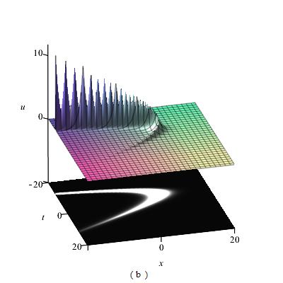
(b) $\lambda=\frac{1}{4}$

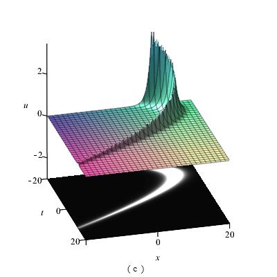
(c) $\lambda=\frac{1}{10}$

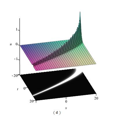
(d) $\lambda=\frac{1}{15}$

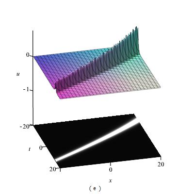
(e) $\lambda=\frac{1}{30}$

(f) $\lambda=0$

Figure 1: (a)$\lambda=1$; (b)$\lambda=\frac{1}{4}$; (c)$\lambda=\frac{1}{10}$; (d)$\lambda=\frac{1}{15}$; (e)$\lambda=\frac{1}{30}$; (f)$\lambda=0$.

Note that $(1-\partial_{xx})u=\delta_{0}\in\mathcal{M}\hookrightarrow B^{0}_{1,\infty}\hookrightarrow B^{-\frac{1}{2}}_{1,\infty},$ where $\mathcal{M}$ is bounded measures spaces. Thanks to $B^{\frac{3}{2}}_{2,\infty}\hookrightarrow H^{1}(\mathbb{R})$, we get $u\in H^{1}(\mathbb{R}).$ Hence, $k(t,x)$ is a conservative solution of equation (1.1) in $H^{1},$ in other words, $u(t,x)$ is a conservative solution in time weighted $H^{1}$ space. Moreover, we infer that

$$\lim\limits_{\lambda\rightarrow 0}q(t)=q(0).$$

∎

6 Uniqueness of solutions for the original equation

In this section, we consider the uniqueness solutions for (2.1). Our main result is as follows.

Theorem 6.1.

Let $k(t,x)\in H^{1}$ be a conservative weak solutions to the Cauchy problem (2.1) in the sense of Definition 2.2. Then $k(t,x)$ is unique.

6.1 Uniqueness of characteristic

This subsection is devoted to the study of the uniqueness of the characteristic to (2.1). Let $k=k(t,x)$ be a conservative solution of (2.1) and satisfy (2.6). Let $y(t,\xi)$ still denote the characteristic

$$\left\{\begin{aligned} &y_{t}(t,\xi)=e^{-\lambda t}k(t,y(t))+\Gamma,\\ &y(0,\xi)=\bar{y}.\end{aligned}\right.$$ (6.1)

Introduce new coordinates $(t,\beta)$ relative to the original coordinates $(t,x)$ by the following transformation

$$y(t,\beta)+\int_{-\infty}^{y(t,\beta)}k_{x}^{2}(t,z)dz=\beta.$$ (6.2)

At time $t$ where the measure $\mu_{(t)}$ is not absolutely continuous with respect to the Lebesgue measure, For any time $t$ and $\beta\in\mathbb{R}$, define $y(t,\beta)$ to be the unique $y$ such that

$$y(t,\beta)+\mu_{(t)}\{(-\infty,y)\}\leq\beta\leq y(t,\beta)+\mu_{(t)}\{(-\infty,y]\}.$$ (6.3)

Combining (3.26) and (6.1), we get

$$\frac{d}{dt}\int_{-\infty}^{y(t)}k_{x}^{2}dx=\int_{-\infty}^{y(t)}2k_{x}(e^{{-\lambda}t}k^{2}-H(k)-P)dx.$$ (6.4)

Now we give the following lemma to prove the Lipschitz continuity of $x$ and $k$ as functions of the variables $t,\beta.$

Lemma 6.2.

Let $k(t,x)$ be a conservative solution of (2.1). Then, for all $t\geq 0$, the following maps

$$\beta\mapsto y(t,\beta),$$

$$\beta\mapsto k(t,y(t,\beta)),$$

defined by (6.3), are Lipschitz continuous with constant $1.$ Moreover, the map $t\mapsto y(t,\beta)$ is also Lipschitz continuous with a constant depending only on $\|\bar{k}\|_{H^{1}}.$

Proof.

Step 1. For any fixed time $t\geq 0$, the map

$$x\mapsto\beta(t,y):=x+\int_{-\infty}^{x}k_{x}^{2}(t,y)dy$$

is right continuous and strictly increasing. This means the inverse $\beta\mapsto x(t,\beta)$ is well-defined, continuous, nondecreasing. Given ${\beta}_{1}<{\beta}_{2}$, we have

$$y(t,{\beta}_{2})-y(t,{\beta}_{1})=({\beta}_{2}-{\beta}_{1})-\int_{y(t,{\beta}_{1})}^{y(t,{\beta}_{2})}k_{x}^{2}(t,z)dz\leq{\beta}_{2}-{\beta}_{1}.$$

One can conclude that $\beta\mapsto y(t,\beta)$ is Lipschitz continuous.

Step 2. Let ${\beta}_{1}<{\beta}_{2}$. Then, it follows that

$$|k(t,{\beta}_{2})-k(t,{\beta}_{1})| \leq\int_{y(t,{\beta}_{1})}^{y(t,{\beta}_{2})}|k_{x}(t,z)|dz\leq\int_{y(t,{\beta}_{1})}^{y(t,{\beta}_{2})}\frac{1}{2}(1+k_{x}^{2})dz$$

$$\leq\frac{1}{2}[y(t,{\beta}_{2})-y(t,{\beta}_{1})+\int_{y(t,{\beta}_{1})}^{y(t,{\beta}_{2})}k_{x}^{2}(t,z)]dz\leq{\beta}_{2}-{\beta}_{1}.$$

Therefore, we arrive at the map $\beta\mapsto k(t,y(t,\beta))$ is Lipschitz continuous.

Step 3. According to (2.5), we have

$$\|2[e^{{-\lambda}t}k^{2}-P-H(k)]k_{x}\|_{L^{1}}\leq\|-H(k)+e^{{-\lambda}t}k^{2}-P\|_{L^{2}}\|k_{x}\|_{L^{2}}\leq C_{E_{0}}.$$

If $t>\tau,$ we obtain

$${\mu}_{t}\{(-\infty,y-C_{E_{0}}(t-\tau))\}\leq {\mu_{\tau}}\{(-\infty,y)\}+\int_{\tau}^{t}\|2[e^{{-\lambda}t}k^{2}-P-H(k)]k_{x}\|_{L^{1}}dt$$

$$\leq {\mu_{\tau}}\{(-\infty,y)\}+C_{E_{0}}(t-\tau).$$

Defining $y^{-}(t):=y-C_{E_{0}}(t-\tau),$ we get

$$y^{-}(t)+{\mu}_{t}\{(-\infty,y^{-}(t)]\} \leq y-C_{E_{0}}(t-\tau)+{\mu}_{\tau}\{(-\infty,y)\}+C_{0}(t-\tau)$$

$$\leq y+{\mu}_{\tau}\{(-\infty,y)\}\leq\beta,$$

which implies $y(t,\beta)\geq y^{-}(t).$

Likewise, defining $y^{+}(t):=y+C_{E_{0}}(t-\tau),$ it follows that

$$y^{+}(t)+{\mu}_{(t)}\{(-\infty,y^{+}(t)]\} \geq y+C_{E_{0}}(t-\tau)+{\mu}_{\tau}\{(-\infty,y)\}+C_{E_{0}}(t-\tau)$$

$$\geq y+{\mu}_{\tau}\{(-\infty,y)\}\geq\beta.$$

Hence, we deduce that $y(t,\beta)\leq y^{+}(t):=y+C_{E_{0}}(t-\tau).$ ∎

Lemma 6.3.

Let $k(t,x)\in H^{1}(\mathbb{R})$ be a conservative solution of the Cauchy problem (2.1). Then, for any $\bar{y}(\xi)\in\mathbb{R},$ there exists a unique Lipschitz continuous map $t\mapsto y(t,\beta):=y(t,\beta(t,\xi))$ which satisfies both (6.1) and (6.4), where $y(t,\beta)$ is the solution of (6.1). Moreover, for any $0\leq\tau\leq t$ one has

$$k(t,y(t))-k(\tau,y(\tau))=-\int_{\tau}^{t}P_{x}(s,y(s))ds.$$ (6.5)

Proof.

Step 1. Assume that $y(t)$ is the characteristic beginning at $\bar{y}(\xi)=\xi\in\mathbb{R}$, which is defined as $t\rightarrow y(t)=y(t,\beta(t)),$ the map $\beta(\cdot)$ is to be determined. Let $y(t)$ be the solution of (6.1) and (6.4). For $t\notin\mathcal{N},$ we have

$$\beta(t,\xi)= y(t)+\int_{0}^{y(t)}k_{x}^{2}(z)dz$$

$$= \int_{0}^{t}\frac{d}{ds}(y(s)+\int_{0}^{y(s)}k_{x}^{2}(s,z)dz)ds+\bar{y}(\xi)+\int_{-\infty}^{\bar{y}(\xi)}\bar{k}_{x}^{2}(z)dz$$

$$= \bar{y}+\int_{0}^{\bar{y}(\xi)}\bar{k}_{x}^{2}(z)dz+\int_{0}^{t}\Gamma+\{\int_{-\infty}^{y(t)}\Big{(}e^{{-\lambda}t}k_{x}+2k_{x}(e^{{-\lambda}t}k^{2}-P-H(k))\Big{)}(s,z)dz\}ds.$$ (6.6)

Set

$$F(t,\beta(t,\xi))\triangleq\Gamma+\int_{-\infty}^{y(t,\beta(t,\xi))}\Big{(}e^{{-\lambda}t}k_{x}+2k_{x}(e^{{-\lambda}t}k^{2}-P-H(k))\Big{)}dy=\xi,$$ (6.7)

and

$$\bar{\beta}(t,\xi)\triangleq\bar{y}(\xi){+}\int_{\infty}^{\bar{y}}\bar{k}_{x}^{2}dy=\xi.$$ (6.8)

According to (6.1)-(6.8), it follows that

$$\beta(t,\xi)=\xi+\int_{0}^{t}F(s,\beta(s,\xi))ds.$$ (6.9)

Step 2. Since $\|k\|_{H^{1}}=\|\bar{k}\|_{H^{1}},$ $y_{\beta}=\frac{1}{1+k^{2}_{x}}$ and the map $\beta\mapsto k(t,y(t,\beta))$ is Lipschitz continuous, we get

$$F_{\beta}=\{e^{{-\lambda}t}k_{x}+2k_{x}[e^{{-\lambda}t}k^{2}-P-H(k)]\}y_{\beta}=\frac{e^{{-\lambda}t}k_{x}+2k_{x}[e^{{-\lambda}t}k^{2}-P-H(k)]}{1+k_{x}^{2}}.$$

It follows that

$$\|F_{\beta}\|_{L^{\infty}}\leq C_{E_{0}}.$$

Moreover

$$|F(s,{\beta}_{2})-F(s,{\beta}_{1})|\leq C_{E_{0}}|{\beta}_{2}-{\beta}_{1}|.$$ (6.10)

Then, the map $\beta\mapsto F(t,\beta(t))$ is Lipschitz continuous. Moreover, the map $\xi\mapsto\beta(t,\xi)$ is strictly monotonic and Lipschitz continuous. From (6.10), we get

$$|\beta(t,{\xi}_{2})-\beta(t,{\xi}_{1})| \leq|{\xi}_{2}-{\xi}_{1}|+\int_{0}^{t}|F(s,\beta(s,{\xi}_{2}))-F(s,\beta(s,{\xi}_{2}))|ds$$

$$\leq|{\xi}_{2}-{\xi}_{1}|+C_{E_{0}}\int_{0}^{t}|\beta(t,{\xi}_{2})-\beta(t,{\xi}_{1})|.$$

The Gronwall inequality ensures that

$$|\beta(t,{\xi}_{2})-\beta(t,{\xi}_{1})|\leq|{\xi}_{2}-{\xi}_{1}|e^{C_{E_{0}}t}.$$

Consequently, for any $\xi_{2}>\xi_{1},$ we get

$$\beta(t,{\xi}_{2})-\beta(t,{\xi}_{1})={\xi}_{2}-{\xi}_{1}+\int_{0}^{t}F(s,\beta(s,{\xi}_{2}))-F(s,\beta(s,{\xi}_{2}))ds\geq({\xi}_{2}-{\xi}_{1})(1-C_{E_{0}}t),$$

which means that monotonicity makes sense as $t$ sufficiently small and the solution $\beta(\cdot)$ of the integral equation (6.9) depends Lipschitz continuously on the initial data. Without loss of generality, assume that $t$ is enough small, otherwise we can use the continuous method. In addition, the map $\xi\mapsto F(t,y(t,\beta(t,\xi)))$ is also Lipschitz continuous.

Step 3. Owing to $F$ is uniformly Lipschitz continuous, we can check that existence and uniqueness of solution of (6.9) by the fixed point theorem. We introduce the Banach space of all continuous function $\beta:{\mathbb{R}}^{+}\rightarrow\mathbb{R}$ with weighted norm

$$\|\beta\|:=\sup\limits_{t\geq 0}e^{-2Ct}|\beta(t)|.$$

For this space, we see that the Picard map

$$(\mathbb{P}\beta)(t)=\bar{\beta}+\int_{0}^{t}F(s,\beta(s))ds$$

is a strict contraction. If $\|{\beta}_{2}-{\beta}_{1}\|=h>0$, we obtain

$$|{\beta}_{2}(s)-{\beta}_{1}(s)|\leq he^{2Cs}.$$

Then, we deduce that

$$|(\mathbb{P}{\beta}_{2})(t)-(\mathbb{P}{\beta}_{1})(t)|\leq\int_{0}|F(s,{\beta}_{2})-F(s,{\beta}_{1})|ds\leq C\int_{0}^{t}|{\beta}_{2}-{\beta}_{1}|ds\leq|\int_{0}^{t}Che^{2Cs}ds|\leq\frac{h}{2}e^{2Ct}.$$

This means $\|(\mathbb{P}{\beta}_{2})(t)-(\mathbb{P}{\beta}_{1})(t)\|\leq\frac{h}{2}.$ The contraction mapping principle guarantees that (6.9) has a unique solution. Thanks to the arbitrary of the $T,$ we infer that the integral equation (6.9) has a unique solution on ${\mathbb{R}}^{+}.$

Step 4. Combining (6.1) and the integral equation (6.9), we infer that the uniqueness of $x(t,\beta)$ depends on the uniqueness of $\beta(t,\xi).$ From the previous analysis, the map $t\mapsto y(t)=y(t,\beta(t,\xi))$ provides the unique solution to (6.9). Owing to $\beta(t)$ and $x(t,\beta(t,\xi))$ are Lipschitz continuous, then $\beta(t,\xi)$ and $x(t)$ are differentiable a.e. Next, we need to prove that (6.1) satisfies (6.1). Indeed, at any $\tau>0,$ we have

(1) $y(\tau)$ is differentiable at $t=\tau;$

(2) the measure ${\mu}_{(\tau)}$ is absolutely continuous.

We argue by contradiction, assume that $(1)$ does not hold, we get ${y}^{\prime}(\tau)\neq e^{{-\lambda}\tau}k(\tau,y(\tau))+\Gamma$. Then, there exists some $\epsilon_{0}>0,$ such that

$${y}^{\prime}(\tau)=e^{{-\lambda}\tau}k(\tau,y(\tau))+\Gamma+2{\epsilon}_{0}.$$ (6.11)

Therefore, for $\delta>0$ sufficiently small, it follows that

$$y^{+}(t):=y(\tau)+(t-\tau)[e^{{-\lambda}t}k(\tau,y(\tau))+\Gamma+\epsilon_{0}]<y(t),~{}for~{}t\in(\tau,\tau+\delta].$$ (6.12)

The approximation argument guarantees that (2.8) remain hold for any test function $\phi\in H^{1}(\mathbb{R})$ with compact support. For any $\epsilon>0$ enough small, we give the following functions

$$\varrho^{\varepsilon}(s,y)=\left\{\begin{array}[]{rcl}0,&y\leq-{\varepsilon}^{-1},\\ y+{\varepsilon}^{-1},&~{}~{}-{\varepsilon}^{-1}\leq y\leq 1-{\varepsilon}^{-1},\\ 1-{\varepsilon}^{-1}(y-y(s)),&~{}~{}~{}~{}~{}~{}y^{+}(s)\leq y\leq y^{+}(s)+\varepsilon,\\ 0,&~{}~{}~{}~{}~{}~{}y\geq y^{+}(s)+\varepsilon,\end{array}\right.$$ (6.13)

$$\chi^{\varepsilon}(s)=\left\{\begin{array}[]{rcl}0,&~{}~{}~{}~{}~{}~{}~{}~{}~{}~{}s\leq\tau-{\varepsilon}^{-1},\\ {\varepsilon}^{-1}(s-\tau+\varepsilon),&~{}~{}\tau-{\varepsilon}\leq s\leq\tau,\\ 1-{\varepsilon}^{-1}(s-t),&~{}~{}t\leq s\leq t+\varepsilon,\\ 0,&~{}~{}~{}~{}~{}~{}~{}s\geq t+\varepsilon.\end{array}\right.$$ (6.14)

Define

$$\phi^{\varepsilon}(s,y)=\min\{{\varrho^{\varepsilon}(s,y),\chi^{\varepsilon}(s)}\}.$$

Let ${\phi}^{\varepsilon}$ be the test function in (2.8). Therefore, one has

$$\int_{\mathbb{R}^{+}}\int_{\mathbb{R}}k^{2}_{x}\phi^{\varepsilon}_{t}+(e^{{-\lambda}t}k+\Gamma)k^{2}_{x}{\phi}_{x}^{\varepsilon}+2(e^{{-\lambda}t}k^{2}-P-H(k)))\phi^{\varepsilon}dxdt=0,$$

which means

$$\int_{\tau-\varepsilon}^{t+\varepsilon}\int_{-{\varepsilon}^{-1}}^{y^{+}(s)-\varepsilon}k^{2}_{x}\phi^{\varepsilon}_{t}+((e^{{-\lambda}t}k^{2}-P-H(k))))\phi^{\varepsilon}dydt=0.$$ (6.15)

If $t$ is sufficiently close to $\tau,$ we have

$$\lim\limits_{\varepsilon\rightarrow 0}\int_{\tau}^{t}\int_{y^{+}(s)-\varepsilon}^{y^{+}(s)+\varepsilon}k^{2}_{x}[\phi^{\varepsilon}_{t}+(e^{{-\lambda}t}k+\Gamma)\phi^{\varepsilon}_{x}](s,x)dy)ds\geq 0.$$

Using the fact that $e^{{-\lambda}s}k(s,y(s))<e^{{-\lambda}\tau}k(\tau,y(\tau))+{\epsilon}_{0}$ and ${\phi}_{x}^{\epsilon}\leq 0.$ For any $s\in[\tau+\varepsilon,t-\varepsilon],$ we infer that

$$0={\phi}_{t}^{\varepsilon}+[e^{{-\lambda}\tau}k^{2}(\tau,y(\tau))+\Gamma]{\phi}_{x}^{\varepsilon}\leq{\phi}_{t}^{\varepsilon}+(e^{{-\lambda}s}k(s,y(s))+\Gamma){\phi}_{x}^{\varepsilon}.$$ (6.16)

Noticing that the family of measures ${\mu}_{t}$ depends continuously on $t$ in the topology of weak convergence, taking the limit of (6.15) as $\epsilon\rightarrow 0$, we obtain

$$0= \int_{-\infty}^{y(\tau)}k^{2}_{x}(\tau,y)dy-\int_{-\infty}^{y^{+}(t)}k^{2}_{x}(t,y)dy+\int_{\tau}^{t}\int_{-\infty}^{y^{+}(s)}2k_{x}((e^{{-\lambda}t}k^{2}-P-H(k))))\phi^{\varepsilon}(s,y)dyds$$

$$+\lim\limits_{\varepsilon\rightarrow 0}\int_{\tau}^{t}\int_{{y^{+}}(s)-\varepsilon}^{{y^{+}}(s)+\varepsilon}k^{2}_{x}[\phi^{\varepsilon}_{t}+(e^{{-\lambda}t}k+\Gamma)\phi^{\varepsilon}_{x}](s,y)dyds$$

$$\geq \int_{-\infty}^{y(\tau)}k^{2}_{x}(\tau,y)dy-\int_{-\infty}^{y^{+}(t)}k^{2}_{x}(t,y)dy+\int_{\tau}^{t}\int_{-\infty}^{y(s)}2k_{x}(((e^{{-\lambda}t}k^{2}-P-H(k)))))\phi^{\varepsilon}(s,y)dyds$$

$$+\underbrace{\int_{\tau}^{t}\int_{y(s)}^{{y^{+}}(s)}2k_{x}(e^{{-\lambda}t}k^{2}-P-H(k))\phi^{\varepsilon}(s,y)dyds}_{o_{1}(t-\tau)}.$$ (6.17)

That is

$${\mu}_{t}\{(-\infty,{y}^{+}(t)]\}\geq {\mu}_{\tau}\{(-\infty,{y}(\tau)]\}+\int_{\tau}^{t}\int_{-\infty}^{y(s)}2k_{x}(e^{{-\lambda}t}k^{2}-P-H(k))\phi^{\varepsilon}(s,y)dyds+o_{1}(t-\tau).$$

From (6.12) and the map $t\mapsto y(t)$ is Lipschitz continuity, we have

$$|o_{1}(t-\tau)|\leq \|2(e^{{-\lambda}t}k^{2}-P-H(k))\|_{L^{\infty}}\int_{\tau}^{t}\int_{{y}(s)}^{{y}^{+}(s)}|k_{x}(s,y)|dyds$$

$$\leq \|2(e^{{-\lambda}t}k^{2}-P-H(k)\|_{L^{\infty}}\|k_{x}\|_{L^{2}}\int_{\tau}^{t}(y(s)-{y}^{+}(s))^{\frac{1}{2}}ds$$

$$\leq C(t-\tau)^{\frac{3}{2}},$$ (6.18)

where $o_{1}(t-\tau)$ satisfies $\frac{o_{1}(t-\tau)}{t-\tau}\rightarrow 0$ as $t\rightarrow\tau$ and $C$ depend on $E_{0}.$
Combining (6.9), (6.12) and (6.1)-(6.1), for $t$ being close enough to $\tau$, we have

$$\beta(t)= \beta(\tau)+(t-\tau)\Big{(}e^{{-\lambda}t}k(\tau,y(\tau))+\Gamma+\int_{-\infty}^{{y}(\tau)}2k_{x}[-e^{{-\lambda}t}k^{2}-P-H(k)](s,y)dyds\Big{)}+o_{2}(t-\tau)$$

$$= y(t)+{\mu}_{t}\{(-\infty,{y}(t)]\}$$

$$> y(\tau)+(t-\tau)[e^{{-\lambda}t}k(\tau,y(\tau))+\Gamma+{\epsilon}_{0}]+{\mu}_{\tau}\{(-\infty,{y}(\tau)]\}$$

$$+\int_{\tau}^{t}\int_{-\infty}^{{y}(s)}2k_{x}[(e^{{-\lambda}t}k^{2}-P-H(k))]dyds+o_{1}(t-\tau).$$ (6.19)

with $o_{2}(t-\tau)$ satisfies $\frac{o_{1}(t-\tau)}{t-\tau}\rightarrow 0$ as $t\rightarrow\tau.$ From (6.1), we have

$$~{}~{}~{}(t- \tau)\Big{(}\int_{-\infty}^{{y}(\tau)}2k_{x}[e^{{-\lambda}t}k^{2}-P-H(k)](s,y)dy\Big{)}+o_{2}(t-\tau)$$

$$\geq(t-\tau){\epsilon}_{0}+\int_{\tau}^{t}\int_{-\infty}^{{y}(s)}2k_{x}[e^{{-\lambda}t}k^{2}-P-H(k)](s,y)dyds+o_{1}(t-\tau).$$

Dividing both sides by $t-\tau$ and letting $t\rightarrow\tau$, one has ${\epsilon}_{0}<0,$ which contradicts with ${\epsilon}_{0}>0$. In addition, for the case ${\epsilon}_{0}<0,$ we follow the similar strategy as ${\epsilon}_{0}>0$. Hence, we conclude that $y(t)$ is differentiable at $t=\tau.$

Step 5. It follows from Definition 2.1 that

$$\int_{\mathbb{R}^{+}}\int_{\mathbb{R}}k\phi_{t}+\frac{(e^{{-\lambda}t}k+\Gamma)}{2}k_{x}{\phi}_{x}+P_{x}\phi_{x}dxdt+\int_{{\mathbb{R}}}\bar{k}(x){\phi}(0,x)dx=0,$$ (6.20)

for any test function $\phi\in C_{c}^{\infty}.$ The approximation argument guarantees that the equation (6.20) remains hold, for any test function $\psi$ which is Lipschitz continuous with compact support. Note that the map $y\rightarrow k(t,y)$ is absolutely continuous and integrate by parts with respect to $x$. Therefore, for any $\varphi\in C_{c}^{\infty}$, taking $\phi={\varphi}_{x}$. we have

$$\int_{\mathbb{R}^{+}}\int_{\mathbb{R}}k_{x}\varphi_{t}+(e^{{-\lambda}t}k+\Gamma)k_{x}{\varphi}_{x}-P_{x}\varphi_{x}dxdt+\int_{{\mathbb{R}}}\bar{k}_{x}(x){\varphi}(0,x)dx=0.$$ (6.21)

For any $\epsilon\geq 0$ sufficiently small, we give the following function

$$\varrho^{\varepsilon}(s,y)=\left\{\begin{array}[]{rcl}0,&~{}~{}~{}~{}y\leq-{\varepsilon}^{-1},\\ y+{\varepsilon}^{-1},&~{}~{}~{}~{}~{}~{}-{\varepsilon}^{-1}\leq y\leq 1-{\varepsilon}^{-1},\\ 1,&1-{\varepsilon}^{-1}\leq y\leq y(s),\\ 1-{\varepsilon}^{-1}(y-y(s)),&~{}~{}~{}~{}~{}~{}~{}~{}~{}y(s)\leq y\leq y(s)+\varepsilon,\\ 0&~{}~{}~{}~{}~{}~{}~{}~{}y\geq y(s)+\varepsilon,\end{array}\right.$$

and

$$\psi^{\varepsilon}(s,y)=\min\{{\varrho^{\varepsilon}(s,y),\chi^{\varepsilon}(s)}\},$$

where $\chi^{\varepsilon}$ is defined in (6.14). Let $\varphi=\psi^{\varepsilon}$ and $\epsilon\rightarrow 0$. Then, it follows from the continuity property of function $P_{x}$ that

$$\int_{-\infty}^{y(t)}k_{x}(t,y)dy =\int_{-\infty}^{y(\tau)}k_{x}(\tau,y)dy-\int_{\tau}^{t}P_{x}(s,y(s))ds$$

$$~{}~{}~{}+\lim\limits_{\varepsilon\rightarrow 0}\int_{\tau-\varepsilon}^{t+\varepsilon}\int_{{y}(s)}^{{y}(s)+\varepsilon}k_{x}[{\psi}_{t}^{\varepsilon}+(e^{{-\lambda}t}k+\Gamma){\psi}_{x}^{\varepsilon}]dyds.$$

Hence, it is shown that

$$\lim\limits_{\varepsilon\rightarrow 0}\int_{\tau-\varepsilon}^{t+\varepsilon}\int_{{y}(s)}^{{y}(s)+\varepsilon}k_{x}[{\psi}_{t}^{\varepsilon}+(e^{{-\lambda}t}k+\Gamma){\psi}_{x}^{\varepsilon}]dyds$$

$$=\lim\limits_{\varepsilon\rightarrow 0}\Big{(}\int_{\tau-\varepsilon}^{\tau}+\int_{\tau}^{t}+\int_{t}^{t+\varepsilon}\Big{)}\int_{{y}(s)}^{{y}(s)+\varepsilon}k_{x}[{\psi}_{t}^{\varepsilon}+(e^{{-\lambda}t}k+\Gamma){\psi}_{x}^{\varepsilon}]dyds=0.$$ (6.22)

First, we claim that

$$\lim\limits_{\varepsilon\rightarrow 0}\int_{\tau}^{t}\int_{{y}(s)}^{{y}(s)+\varepsilon}k_{x}[{\psi}_{t}^{\varepsilon}+(e^{{-\lambda}t}k+\Gamma){\psi}_{x}^{\varepsilon}]dyds=0.$$

Taking advantage of Cauchy’s inequality and $k_{x}\in L^{2}$, one has

$$|\int_{\tau-\varepsilon}^{t}\int_{{y}(s)}^{{y}(s)+\varepsilon}k_{x}[{\psi}_{t}^{\varepsilon}+(e^{{-\lambda}t}k+\Gamma){\psi}_{x}^{\varepsilon}]dyds|$$

$$\leq\int_{\tau-\varepsilon}^{t}\Big{(}\int_{{y}(s)}^{{y}(s)+\varepsilon}|k_{x}|^{2}dy\Big{)}^{\frac{1}{2}}\Big{(}\int_{{y}(s)}^{{y}(s)+\varepsilon}[{\psi}_{t}^{\varepsilon}+(e^{{-\lambda}t}k+\Gamma){\psi}_{x}^{\varepsilon}]^{2}dy\Big{)}^{\frac{1}{2}}ds.$$

Define

$${\pi}_{\varepsilon}(s)=\Big{(}\sup\limits_{x\in\mathbb{R}}\int_{{y}(s)}^{{y}(s)+\varepsilon}k_{x}^{2}(s,y)dy\Big{)}^{\frac{1}{2}}.$$

Note that the function ${\pi}_{\epsilon}(s)$ is uniformly bounded for $\epsilon$ and $\lim\limits_{\varepsilon\rightarrow 0}{\pi}_{\varepsilon}(s)=0$ almost every time $t.$ Hence, it follows from the dominated convergence theorem that

$$\lim\limits_{\varepsilon\rightarrow 0}\int_{\tau}^{t}\Big{(}\sup\limits_{x\in\mathbb{R}}\int_{{y}(s)}^{{y}(s)+\varepsilon}k_{x}^{2}(s,y)dy\Big{)}^{\frac{1}{2}}ds\leq\lim\limits_{\varepsilon\rightarrow 0}\int_{\tau}^{t}{\pi}_{\varepsilon}(s)ds=0.$$ (6.23)

In addition, for all $s\in[\tau,t]$, one can get from the definition of $\psi_{\epsilon}$ that

$${\psi}_{x}^{\varepsilon}(s,y)=-{\varepsilon}^{-1},\quad{\psi}_{t}^{\varepsilon}(s,y)+(e^{{-\lambda}s}k(s,y(s))+\Gamma){\psi}_{x}^{\varepsilon}(s,y)=0,$$ (6.24)

with $y(s)<y<y(s)+\epsilon.$ Then, it follows from (6.24) that

$$\int_{{y}(s)}^{{y}(s)+\varepsilon}({\psi}_{t}^{\varepsilon}(s,y)+(e^{{-\lambda}s}k(s,x(s))+\Gamma){\psi}_{x}^{\varepsilon}(s,y))^{2}dy$$

$$={\varepsilon}^{-2}\int_{{y}(s)}^{{y}(s)+\varepsilon}(k(s,y)-{k(s,y(s))})^{2}dy$$

$$\leq{\varepsilon}^{-1}\Big{(}\max\limits_{y(s)<y<y(s)+\epsilon}|k(s,y)-{k(s,y(s))}|\Big{)}^{2}$$

$$\leq{\varepsilon}^{-1}\Big{(}\int_{{y}(s)}^{{y}(s)+\varepsilon}|k(s,y)-{k(s,y(s))}|dy\Big{)}^{2}$$

$$\leq{\varepsilon}^{-{\frac{1}{2}}}({\varepsilon}^{{\frac{1}{2}}}\|k_{x}(s)\|_{H^{1}})^{2}\leq C\|k(s)\|_{H^{1}}.$$ (6.25)

Using (6.23) and (6.1), we obtain

$$\lim\limits_{\varepsilon\rightarrow 0}\int_{\tau}^{t}\int_{{y}(s)}^{{y}(s)+\varepsilon}k_{x}[{\psi}_{t}^{\varepsilon}+(e^{{-\lambda}s}k+\Gamma){\psi}_{x}^{\varepsilon}](s,y)dyds=0.$$ (6.26)

The Cauchy-Schwartz inequality and (6.24) entail that

$$\lim\limits_{\varepsilon\rightarrow 0}(\int_{\tau-\varepsilon}^{t}+\int_{t}^{t+\varepsilon})\int_{{y}(s)}^{{y}(s)+\varepsilon}k_{x}[{\psi}_{t}^{\varepsilon}+(e^{{-\lambda}s}k+\Gamma){\psi}_{x}^{\varepsilon}](s,y)dyds$$

$$\leq\lim\limits_{\varepsilon\rightarrow 0}(\int_{\tau-\varepsilon}^{t}+\int_{t}^{t+\varepsilon})\Big{(}\int_{{y}(s)}^{{y}(s)+\varepsilon}|k_{x}|^{2}dy\Big{)}^{\frac{1}{2}}(\int_{{y}(s)}^{{y}(s)+\varepsilon}[{\psi}_{t}^{\varepsilon}+(e^{{-\lambda}s}k+\Gamma){\psi}_{x}^{\varepsilon}]^{2}dy\Big{)}^{\frac{1}{2}}ds$$

$$\leq\lim\limits_{\varepsilon\rightarrow 0}2\epsilon\|k(s)\|_{H^{1}}\Big{(}\int_{{y}(s)}^{{y}(s)+\varepsilon}2{\epsilon}^{-2}\|k\|_{L^{\infty}}^{2}dy\Big{)}^{\frac{1}{2}}$$

$$\leq\lim\limits_{\varepsilon\rightarrow 0}C{\epsilon}^{\frac{1}{2}}=0.$$ (6.27)

Combining (6.26)-(6.1), we arrive at (6.1).

Step 6. Using the uniqueness of $\beta(t,\xi),$ we can deduce that the uniqueness of $y(t,\xi).$ ∎

The following lemma is to prove the Lipschitz continuity of $k$ with respect to $t$ under the Lagrange coordinates.

Lemma 6.4.

Let $k=k(t,x)$ be a conservative solution to (2.1). Then the map $(t,\beta)\mapsto k(t,y(t,\beta))$ is Lipschitz continuous with a constant depending only on the norm $\|\bar{k}\|_{H^{1}}.$

Proof.

Combining (6.7) and (6.9), we get

$$|k(t,y(t,\bar{\beta}))-k(\tau,\bar{\beta})|\leq |k(t,y(t,\bar{\beta}))-k(t,y(t,{\beta}(t)))|+|k(t,y(t,{\beta}(t)))-k(\tau,y(\tau,{\beta}(\tau)))|$$

$$\leq \frac{1}{2}|{\beta}(t)-\bar{\beta}|+(t-\tau)\|P_{x}\|_{L^{\infty}}$$

$$\leq (t-\tau)(\frac{1}{2}\|F\|_{L^{\infty}}+\|P_{x}\|_{L^{\infty}}),$$

which implies the map $(t,\beta)\mapsto k(t,x(t,\beta))$ is Lipschitz continuous. ∎

Lemma 6.5.

Let $k\in H^{1}(\mathbb{R})$ and define the convolution $P$ being as in (2.2). Then $P_{x}$ is absolutely continuous and satisfies

$$P_{xx}=P-\Big{(}-H(k)+e^{-\lambda t}k^{2}+\frac{e^{{-\lambda}t}}{2}k_{x}^{2}\Big{)}.$$ (6.28)

Proof.

The function $\psi(s)=\frac{e^{-|x|}}{2}$ satisfies the distributional identity

$$D^{2}_{x}\psi=\psi-\delta_{0}.$$

Thanks to $\delta_{0}$ denotes a unit Dirac mass at the origin. Thus, for all function $f\in L^{1}(\mathbb{R}),$ the convolution satisfies

$$D^{2}_{x}(\psi\ast f)=\psi\ast f-f.$$

Choosing $f=-H(k)+e^{-\lambda t}k^{2}+\frac{e^{{-\lambda}t}}{2}k_{x}^{2},$ we obtain the desired result. ∎

6.2 Proof of uniqueness

We need to seek a good characteristic, and employ haw the gradient $k_{x}$ of a conservative solution varies along the good characteristic, and complete the proof of uniqueness.

Proof.

Step 1. Lemmas 6.3-6.4 ensure that the map $(t,\xi)\mapsto(y,k)(t,\xi)$ and $\xi\mapsto F(t,\xi)$ are Lipschitz continuous. Thanks to Rademacher’s theorem, the partial derivatives $y_{t},y_{\xi},k_{t},k_{\xi}$ and $F_{\xi}$ exist almost everywhere. Moreover, $y(t,\xi)$ is the unique solution to (5.1), and the following holds.

(GC) For a.e. $\xi$ and a.e. $t\geq 0$, the point $(t,\beta(t,\bar{\beta}))$ is a Lebesgue point for the partial derivatives $y_{t},y_{\xi},k_{t},k_{\xi}$ and $F_{\xi}$. Moreover, $y_{\xi}(t,\xi)>0$ for $a.e.~{}t\geq 0.$

If (GC) holds, then $t\rightarrow y(t,\xi)$ is a good characteristic.

Step 2. We now construct an ODE to describe that the quantities $k_{\xi}$ and $x_{\xi}$ vary along a good characteristic. Supposing that $t,~{}\tau\notin\mathcal{N},$ and $y(t,\xi)$ is a good characteristic, we then have

$$y(t,\beta(t,\xi))=\bar{y}(\xi)+\int_{0}^{t}(e^{-\lambda s}k(s,\beta(s,\xi))+\Gamma)ds.$$

Differentiating the above equation with respect to $\xi$, we deduce that

$$y_{\xi}=\bar{y}_{\xi}(\xi)+\int_{0}^{t}k_{\xi}(s,\xi)d\xi.$$ (6.29)

Likewise, we have

$$k_{\xi}=\bar{k}_{x}(\bar{y}(\xi))\bar{y}_{\xi}-\int_{0}^{t}G_{\xi}(s,\xi)d\xi.$$ (6.30)

From (6.29)-(6.30), we end up with

$$\left\{\begin{aligned} &y_{t\xi}=e^{-\lambda t}k_{\xi},\\ &k_{t\xi}=-G_{\xi}.\end{aligned}\right.$$ (6.31)

Step 3. We now return to the original coordinates $(t,x)$ and derive an evolution equation for the partial derivative $k_{x}$ along a “good” characteristic curve. For a fixed point $(t,x)$ with $t\notin\mathcal{N}$. Suppose that $\bar{x}$ is a Lebesgue point for the map $x\rightarrow k_{x}(t,x)$, and $\xi$ satisfies $x=y(t,\xi),$ and suppose that $t\rightarrow y(t,\xi)$ is a good characteristic, which implies (GC) holds. From (6.1) we have

$$y_{\beta}(t,\beta)=\frac{1}{1+k^{2}_{x}(t,y)}>0,\ \beta(t,\xi)>0,$$ (6.32)

which implies that $y_{\xi}(t,\xi)>0.$

Hence, the partial derivative $k_{x}$ can be calculated as shown below

$$k_{x}(t,y(t,\beta(t;\tau,\bar{\beta})))=\frac{k_{\xi}(t,y(t,\beta(t,{\xi})))}{y_{\xi}(t,\beta(t;\bar{\xi}))}.$$

Applying (6.31) to describe the evolution of $k_{\xi}$ and $y_{\xi},$ we infer that the map $t\rightarrow k_{x}(t,y(t,\beta(t,{\xi})))$ is absolutely continuous. It follows that

$$\frac{d}{dt}k_{x}(t,y(t,\beta(t;\tau,{\xi}))) =\frac{d(\frac{k_{\xi}}{y_{\xi}})}{dt}=\frac{y_{\xi}F_{\xi}-e^{-\lambda t}{k_{\xi}}^{2}}{{y_{\xi}}^{2}}.$$

Hence, we conclude that as long as $y_{\beta}\neq 0$, the map $t\rightarrow k_{x}$ is absolutely continuous.

Step 4. Let

$$K(t,\xi)=k(t,y(t,\xi)),\quad V(t,\xi)=\frac{k_{x}^{2}\circ y}{1+k_{x}^{2}\circ y},$$

$$W(t,\xi)=\frac{k_{x}\circ y}{1+k_{x}^{2}\circ y},\quad Q(t,\xi)=({1+k_{x}^{2}\circ y})\cdot y_{\xi}.$$

From which it follows that

$$\left\{\begin{aligned} y_{t}&=e^{{-\lambda}t}K+\Gamma,\\ K_{t}&=-G,\\ V_{t}&=2W\Big{(}e^{{-\lambda}t}K^{2}(1-V)-H(K)(1-V)-\frac{e^{{-\lambda}t}}{2}V-{P}(1-V)\Big{)},\\ W_{t}&=(1-2V)\Big{(}e^{{-\lambda}t}K^{2}(1-V)-H(K)(1-V)-\frac{e^{{-\lambda}t}}{2}V-{P}(1-V)\Big{)},\\ Q_{t}&=2WQ\Big{(}\frac{e^{{-\lambda}t}}{2}+e^{{-\lambda}t}K^{2}-H(K)-{P}\Big{)}.\\ \end{aligned}\right.$$ (6.33)

For any $\xi\in\mathbb{R},$ we deduce that the following initial conditions

$$\left\{\begin{aligned} \int_{0}^{\bar{y}}\bar{k}_{x}^{2}&dx+\bar{y}(\xi)=\xi,\\ \bar{K}(\xi)&=\bar{k}\circ\bar{y}(\xi),\\ \bar{V}(\xi)&=\frac{\bar{k}_{x}^{2}\circ\bar{y}}{1+\bar{k}_{x}^{2}\circ\bar{y}(\xi)},\\ \bar{W}(\xi)&=\frac{\bar{k}_{x}\circ\bar{y}(\xi)}{1+\bar{k}_{x}^{2}\circ\bar{y}(\xi)},\\ \bar{Q}(\xi)&=(1+\bar{k}_{x}^{2}\circ\bar{y})\bar{y}_{\xi}(\xi)=1.\\ \end{aligned}\right.$$ (6.34)

Making use of all coefficients is Lipschitz continuous and the previous steps again, the system (6.33)-(6.34) has a unique globally solution.

Step 5. Let $k$ and $\tilde{k}$ be two conservative weak solution of (2.1) with the same initial data $\bar{k}\in H^{1}(\mathbb{R})$ . For $a.e.~{}t\geq 0,$ the corresponding Lipschitz continuous maps $\xi\mapsto y(t,\xi),{\xi}\mapsto\tilde{y}(t,\beta)$ are strictly increasing. Hence they have continuous inverses, say $x\mapsto{y}^{-1}(t,x),x\mapsto{\tilde{y}}^{-1}(t,x)$. Thus, we deduce that

$$y(t,\xi)=\tilde{y}(t,\xi),\ k(t,y(t,\xi))=\tilde{k}(t,{y}(t,\xi)).$$

Moreover, for $a.e.~{}t\geq 0$, we have

$$k(t,x)=k(t,y(t,\xi))=\tilde{k}(t,\tilde{y}(t,\xi))=\tilde{k}(t,x).$$

Then, we finish the proof of Theorem 6.3. ∎

Proof of Theorem 2.3.

Theorem 4.1 and Theorem 6.1 ensure that the equation (2.1) has a unique globally conservative solution. $~{}~{}~{}~{}~{}~{}~{}~{}~{}~{}~{}~{}~{}~{}~{}~{}~{}~{}~{}~{}~{}~{}~{}~{}~{}~{}~{}~{}~{}~{}~{}~{}~{}~{}~{}~{}~{}~{}~{}~{}~{}~{}~{}~{}~{}~{}~{}~{}~{}~{}~{}~{}~{}~{}~{}~{}~{}~{}~{}~{}~{}~{}~{}~{}~{}~{}~{}~{}~{}~{}~{}~{}~{}~{}~{}~{}~{}~{}~{}~{}~{}~{}~{}~{}~{}~{}~{}~{}~{}~{}\square$

Acknowledgements. This work was partially supported by NNSFC (Grant No. 12171493), the FDCT (Grant No. 0091/2018/A3), the Guangdong Special Support Program (Grant No.8-2015).

References

- [1] A. Bressan, A. Constantin, Global conservative solutions of the Camassa-Holm equation. Arch. Ration. Mech. Anal., 183(2):215–239, 2007.
- [2] A. Bressan, A. Constantin, Global dissipative solutions of the Camassa-Holm equation. Anal. Appl., 5(1):1–27, 2007.
- [3] A. Bressan, G. Chen, Q. Zhang, Uniqueness of conservative solutions to the Camassa-Holm equation via characteristics. Discrete Contin. Dyn. Syst., 35(1):25–42, 2015.
- [4] R. Camassa, D. D. Holm, An integrable shallow water equation with peaked solitons. Phys. Rev. Lett., 71(11):1661–1664, 1993.
- [5] A. Constantin, Existence of permanent and breaking waves for a shallow water equation: a geometric approach. Ann. Inst. Fourier (Grenoble), 50(2):321–362, 2000.
- [6] A. Constantin, J. Escher, Global existence and blow-up for a shallow water equation. Ann. Scuola Norm. Sup. Pisa Cl. Sci. (4), 26(2):303–328, 1998.
- [7] A. Constantin, J. Escher, Wave breaking for nonlinear nonlocal shallow water equations. Acta Math., 181(2):229–243, 1998.
- [8] A. Constantin, J. Escher, Well-posedness, global existence, and blowup phenomena for a periodic quasi-linear hyperbolic equation. Comm. Pure Appl. Math., 51(5):475–504, 1998.
- [9] A. Constantin, L. Molinet, Global weak solutions for a shallow water equation. Comm. Math. Phys., 211(1):45–61, 2000.
- [10] A. Constantin, On the scattering problem for the Camassa-Holm equation. R. Soc. Lond. Proc. Ser. A Math. Phys. Eng. Sci., 457(2008):953–970, 2001.
- [11] A. Constantin, D. Lannes, The hydrodynamical relevance of the Camassa-Holm and Degasperis-Procesi equations. Arch. Ration. Mech. Anal., 192(1):165–186, 2009.
- [12] P. L. da Silva, I. L. Freire, Integrability, existence of global solutions, and wave breaking criteria for a generalization of the Camassa-Holm equation. Stud. Appl. Math., 145(3):537–562, 2020.
- [13] R. Danchin, A few remarks on the Camassa-Holm equation. Differential Integral Equations, 14(8):953–988, 2001.
- [14] R. Danchin, A note on well-posedness for Camassa-Holm equation. J. Differential Equations, 192(2):429–444, 2003.
- [15] Y. Guo, W. Ye, Z. Yin, Ill-posedness for the cauchy problem of the Camassa-Holm equation in . J. Differential Equations 327: 127-144, 2022.
- [16] Z. Guo, X. Liu, L. Molinet, Z. Yin, Ill-posedness of the Camassa-Holm and related equations in the critical space. J. Differential Equations, 266(2-3):1698–1707, 2019.
- [17] H. Holden, X. Raynaud, Global conservative solutions of the Camassa-Holm equation—a Lagrangian point of view. Comm. Partial Differential Equations, 32(10-12):1511–1549, 2007.
- [18] I. L. Freire, Wave breaking for shallow water models with time decaying solutions. J. Differential Equations, 269(4):3769–3793, 2020.
- [19] J. Li, Z. Yin, Remarks on the well-posedness of Camassa-Holm type equations in Besov spaces. J. Differential Equations, 261(11):6125–6143, 2016.
- [20] J. Li, Y. Yu, W. Zhu, Ill-posedness for the Camassa-Holm and related equations in Besov spaces. J. Differential Equations, 306:403–417, 2022.
- [21] Y. Li, P. J. Olver, Well-posedness and blow-up solutions for an integrable nonlinearly dispersive model wave equation. J. Differential Equations, 162(1):27–63, 2000.
- [22] Z. Luo, Z. Qiao, Z. Yin, Globally conservative solutions for the modified Camassa-Holm (MOCH) equation. J. Math. Phys., 62(9):Paper No. 091506, 12, 2021.
- [23] Z. Meng, Z. Yin, On the Cauchy problem for a weakly dissipative Camassa-Holm equation in critical Besov spaces. arXiv:2206.05013, 2022.
- [24] Z. Qiao, The Camassa-Holm hierarchy, related n-dimensional integrable systems, and algebro-geometric solution on a symplectic submanifold. Communications in Mathematical Physics, 239(1-2):309–341, 2003.
- [25] G. Rodríguez-Blanco, On the Cauchy problem for the Camassa-Holm equation. Nonlinear Anal., 46(3):309–327, 2001.
- [26] Z. Xin, P. Zhang, On the weak solutions to a shallow water equation. Comm. Pure Appl. Math., 53(11):1411–1433, 2000.
- [27] W. Ye, Z. Yin, Y. Guo, A new result for the local well-posedness of the Camassa-Holm type equations in critial Besov spaces . arXiv: 2101.00803,2021.
- [28] M. Zhou, The Theory of Function of Real Variables. Peking University Press, Beijing, 2008.