Gauss-Bonnet black holes in $(2+1)$ dimensions: Perturbative aspects and entropy features

Abstract

We investigate some aspects of the $(2+1)$-dimensional Gauss-Bonnet black hole proposed in Hennigar et al. (2020a, 2021). The perturbations of scalar and massless spinorial fields are studied suggesting the dynamical stability of the geometry. The field evolution is analyzed calculating the quasinormal modes for different parameters and exploring the influence of the coupling constant of the theory. The hydrodynamical modes are also obtained in the small coupling limit. Furthermore, the entropy bound and the dominant semiclassical correction to the black hole entropy are calculated.

I Introduction

Lower dimensional gravity has been a very active field for a long time in theoretical physics due to both its simplicity and its features, which have a strong similarity to those in the four-dimensional gravity theory. Black hole solutions were found in several lower dimensional models like the well-known $(2+1)$-dimensional BTZ (Bañados-Teitelboim-Zanelli) black hole Banados et al. (1992) and the solutions of Jackiw gravity Jackiw (1985) in $(1+1)$-dimensions among others (for an extensive survey see Mann (1992)). The Gauss-Bonnet (GB) gravity is a particular case of Lovelock theories Lovelock (1971), which includes higher curvature corrections to the Einstein-Hilbert action given in terms of the Riemann tensor. The equations of motion are differential equations of second-order for the metric tensor components. A special feature of those higher-curvature terms is that they are identically zero if the spacetime dimension is bounded by $D<5$.

More recently, a proposal to evade the Lovelock theorem and allow higher-curvature terms, in particular, the GB term, to survive without extra fields for $D<5$ was proposed in Glavan and Lin (2020). Nevertheless, in several papers its was shown that such a proposal leads to an ill-defined theory Gürses et al. (2020); Hennigar et al. (2020b); Arrechea et al. (2021). Despite such inconsonance, it is still possible to include the four-dimensional GB corrections in a consistent way Lu and Pang (2020); Kobayashi (2020), showing that the four-dimensional solution reported in Glavan and Lin (2020) could be obtained from a scalar-tensor theory which is a subclass of Horndeski family Horndeski (1974). Following the same guidelines, a $(2+1)$-dimensional black hole solution with GB correction was found by Henningar et al. Hennigar et al. (2020a, 2021). Such a family of solutions admits a generalization of the BTZ black hole, which is recovered in the limit when the GB coupling goes to zero. In our present work we are interested in a deeper comprehension of those GB-BTZ black holes in $(2+1)$ dimensions, specially in the role that the GB coupling constant plays on the stability when the metric is perturbed by probe fields.

As it is essential to understand in which situations a black hole solution is stable under small perturbations, the study of the field propagation and the determination of the quasinormal spectrum due to probe matter fields in the geometry of the (2+1)-dimensional GB-BTZ black holes can shed some light on this stability. Moreover, the stable or unstable nature of the metric is closely related to the shape of each wave potential Horowitz and Hubeny (2000).

Much work has been done on linear perturbations of GB black holes in different dimensions. Recent studies include the gravitational perturbations and the ringdown phase of black holes in Einstein-dilaton-Gauss-Bonnet gravity in four dimensions Blázquez-Salcedo et al. (2016) and the use of quasi-periodic oscillations to constrain the space of parameters of the theory Maselli et al. (2015). In addition, in Konoplya et al. (2020) the calculation of the black hole shadow radius is implemented in the Einstein-scalar-Gauss-Bonnet gravity with non-trivial scalar hair and in Konoplya and Zinhailo (2020) the quasinormal modes and the stability of the new four-dimensional Gauss-Bonnet black holes were investigated. Moreover, an interesting relation between the shadow radius and quasinormal spectrum was stablished in Jusufi (2020a, b); Cuadros-Melgar et al. (2020). Whether such a relation can be assigned to three-dimensional black holes still remains an open question.

In addition, we are interested in exploring some thermodynamical aspects of the (2+1)-dimensional GB-BTZ black hole. Since the pioneering works of Bekenstein Bekenstein (1973) and Hawking Hawking (1975), which led to the identification of the black hole surface gravity and the event horizon area with the temperature and the entropy of a thermodynamical system, respectively, the black hole thermodynamics has developed and brought different techniques that have improved our understanding of the properties of these remarkable objects. One of these physical quantities is the black hole entropy, which accounts for the maximum entropy a physical system can carry. If an object is captured by a black hole, according to the generalized second law of thermodynamics, the entropy should always increase as well as the event horizon area since they are connected through the Bekenstein-Hawking classical formula, $S_{BH}=Area/4$. Based on this observation, Bekenstein proposed the existence of an upper bound on the entropy of any system Bekenstein (1981) carrying an energy $E$ and with a characteristic dimension $R$, i.e., $S\leq 2\pi ER$, which proved to be universal until nowadays. Along with this subject is the need to include quantum aspects in the description of black hole entropy. In this way, ’t Hooft brought a proposal forward by considering a thermal bath of scalar fields just outside the event horizon so that they could contribute to the entropy provided that a cut-off both close and far from the black hole is included. This technique is known as the brickwall method ’t Hooft (1985) and its calculation leads to a dominant correction also correlated to the event horizon area. In fact, the coefficient of proportionality is universal for each spacetime dimensionality. It is our aim to verify if these properties can be fulfilled by the (2+1)-dimensional GB-BTZ black hole.

The paper is organized as follows. In Sec.II we discuss the main features of $(2+1)$ GB-BTZ black hole solution. In Sec.III we compute the quasinormal modes and frequencies due to a massless scalar probe field and discuss the effect of the GB coupling upon the stability. Sec.IV brings the massless spinorial field as the probe field and the quasinormal modes and spectrum are obtained. In Sec.V the hydrodynamic approximation for the probe scalar field in the limit of small GB coupling constant is considered and its interpretation in terms of gauge/gravity correspondence is discussed. Sec.VI is devoted to some thermodynamical aspects of the black hole solutions. Finally, in Sec.VII, we discuss our results and possible perspectives for future work.

II Gauss-Bonnet black hole solutions in $(2+1)$-dimensions

The action that describes the Gauss-Bonnet (GB) gravity in $(2+1)$-dimensions, encoding the main characteristics of its $(3+1)$-dimensional counterpart, is given by Hennigar et al. (2020a),

$$S=\int d^{3}x\sqrt{-g}\left\{R-2\Lambda+\alpha\left[\phi\mathcal{G}+4G^{ab}\partial_{a}\phi\partial_{b}\phi-4(\partial\phi)^{2}\square\phi+2((\nabla\phi)^{2})^{2}\right]\right\}\,,$$ (1)

where we have the Einstein-Hilbert term plus a cosmological constant $\Lambda$, the corrections coming from the GB term  $\mathcal{G}=R_{abcd}R^{abcd}-4R_{ab}R^{ab}+R^{2}$, being $\alpha$ the GB coupling constant, and an additional scalar field $\phi$. Notice that the same coupling between the Einstein tensor $G_{ab}$ and the kinetic term of $\phi$ is present in the Horndeski theory and, indeed, the theory represented by the action (1) is a special case of Horndeski class Horndeski (1974).

As pointed out in Hennigar et al. (2020a), the GB part of (1) can be obtained at least by two different methods. Namely, a Kaluza-Klein (KK) dimensional reduction of a $D$-dimensional theory compactified on an internal maximally symmetric space that leads to a $D=3$ GB gravity Lu and Pang (2020) and the generalization of Ross-Mann method to obtain the $D\rightarrow 2$ limit of General Relativity Mann and Ross (1993) through a conformal transformation on the metric $\tilde{g_{ab}}=e^{\Psi}g_{ab}$ and an expansion of the action around the spatial dimension of interest. Both methods lead to the action (1) as long as the maximally symmetric space used in the KK approach is flat, otherwise, additional terms are generated Hennigar et al. (2020a),

$$S_{\lambda}=-2\int d^{3}x\sqrt{-g}\left[\lambda e^{-2\phi}\left(R+6(\partial\phi)^{2}\right)+3\lambda^{2}e^{-4\phi}\right]\,,$$ (2)

where $\lambda$ represents the curvature of the internal space.

In order to obtain black hole solutions to the GB gravity in $(2+1)$ dimensions we consider the equations of motion that come from the action (1) together with the additional terms (2) and the following ansatz for the line element Hennigar et al. (2020a),

$$ds^{2}=-f(r)dt^{2}+\frac{1}{f(r)h(r)}dr^{2}+r^{2}\left(d\varphi-\frac{J}{2r^{2}}dt\right)^{2}\,,$$ (3)

where $J$ is a constant. In addition, the scalar field $\phi$ depends only on the radial coordinate, $\phi=\phi(r)$. Then, using this ansatz and varying the action with respect to $f(r)$, $h(r)$, and $\phi(r)$ we obtain three equations of motion, whose simplest solution is the BTZ black hole Banados et al. (1992) when considering $h(r)=1$, $\phi=\hbox{constant}$ and $\lambda=0$,

$$f_{BTZ}(r)=-M+\frac{r^{2}}{L^{2}}+\frac{J}{4r^{2}}\,,$$ (4)

with $M$ and $J$ denoting the black hole mass and angular momentum, respectively, and the cosmological constant $\Lambda$ is related to the curvature radius $L$ by $\Lambda=L^{-2}$.

Furthermore, new black hole solutions in three dimensions depending on the GB coupling are achieved by considering a non-constant scalar field $\phi(r)$. In the static case $J=0$ and setting $\lambda=0$ the equations of motion admit the following solution Hennigar et al. (2020a),

$$f(r)_{\pm}=-\frac{r^{2}}{2\alpha}\left(1\pm\sqrt{1+\frac{4\alpha}{r^{2}}\left(-M+\frac{r^{2}}{L^{2}}\right)}\right)\,,$$ (5)

$$\phi(r)=\ln\left(\frac{r}{L}\right)\,.$$ (6)

The positive branch $f(r)_{+}$ of solution (5) does not have a well-defined limit as the GB coupling constant goes to zero, in fact, in this limit it reduces to

$$f(r)_{+}\approx M-\frac{r^{2}}{L^{2}}-\frac{r^{2}}{\alpha}\,,$$ (7)

which goes to infinity as $\alpha\rightarrow 0$. In this sense, the positive branch does not describe a physical system. Conversely, the negative branch $f(r)_{-}$ reduces to BTZ black hole in the same limit. Also, at large distances the negative branch is described by an AdS-like metric, what yields a condition on the allowed values of the GB coupling in order to have a well-defined solution at spatial infinity, i.e., $\alpha>-L^{2}/4$.

Since the negative branch admits a bounded limit for small $\alpha$ and is well behaved at large distances, we are going to consider only $f(r)_{-}$ as black hole solution and, thus, we will drop the subscript $-$ in $f(r)_{-}$ from now on. As the event horizon $r=r_{+}$ of this metric is the same as that of the BTZ solution, $r_{+}=LM^{1/2}$, we see that the GB coupling does not change the location of the event horizon. Moreover, the near horizon limit of $f(r)$ is given by

$$f(r)\approx\frac{2M^{1/2}}{L}(r-r_{+})+\mathcal{O}((r-r_{+})^{2})\,,$$ (8)

showing that $\alpha$ contributes only for large distances from $r_{+}$.

Furthermore, we can distinguish two cases in the internal geometric structure of the negative branch. When $\alpha>0$, the black hole has a branch singularity analogous to GB higher-dimensional solutions. This singularity can be found by using the condition that the argument of the square root in the metric vanishes, thus we have

$$r_{b}=2L\sqrt{\frac{M\alpha}{L^{2}+4\alpha}}=2\sqrt{\frac{\alpha}{L^{2}+4\alpha}}\,r_{+}<r_{+}\,,$$ (9)

where the last inequality shows that the branch singularity remains inside the event horizon. Around $r_{b}$ the Kretschmann scalar behaves as

$$K\equiv R_{\alpha\beta\mu\nu}R^{\alpha\beta\mu\nu}\sim\frac{r_{b}^{3}(L^{2}+4\alpha)}{32\alpha^{2}L^{2}(r-r_{b})^{3}}+\cdots\,.$$ (10)

This type of divergence is the same found in higher-dimensional GB solutions Torii and Maeda (2005) and shows that $r_{b}$ is a true curvature singularity.

On the other hand, when $-L^{2}/4<\alpha<0$, the metric continues until $r=0$, where the Kretschmann scalar behaves as

$$K\sim-\frac{2M}{\alpha r^{2}}+\cdots\,,$$ (11)

showing that at $r=0$ a curvature singularity is located.

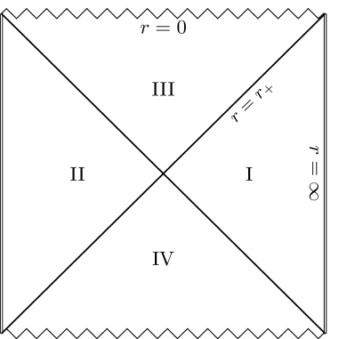
The Kruskal-Szekeres extension of black solution (5) and its Penrose-Carter diagram can be constructed by a detailed examination of the metric near the event horizon $r=r_{+}$ and at spatial infinity $r\rightarrow\infty$.

Near the event horizon it is possible to approximate the function $f(r)$ as $f(r)\approx 2\kappa_{+}(r-r_{+})$, where $\kappa_{+}=f^{\prime}(r_{+})/2$, and in this region the tortoise coordinate $r_{*}$ can be written as

$$r_{*}\approx\frac{1}{\kappa_{+}}\ln{|\kappa_{+}(r-r_{+})|}.$$ (12)

Defining a double null system of coordinates, $U_{+}=t-r_{*}$ and $V_{+}=t+r_{*}$, we obtain the Kruskal-Szekeres extension near the event horizon,

$$U_{+}V_{+}=\mp\kappa_{+}|(r-r_{+})|,$$ (13)

in which the minus sign refers to the region $r>r_{+}$ and the plus sign corresponds to the region $r<r_{+}$.

At spatial infinity $r\rightarrow\infty$ the Kruskal-Szekeres extension reads

$$U_{\infty}V_{\infty}=-e^{\frac{2}{L^{2}r^{2}}}.$$ (14)

Combining each extension (13)-(14) through the Penrose coordinates $T=\frac{1}{2}(\tilde{U}+\tilde{V})$ and $R=\frac{1}{2}(\tilde{U}-\tilde{V})$ with $\tilde{U}=\arctan(U)$ and $\tilde{V}=\arctan(V)$, we accomplish the Penrose-Carter diagrams for the entire spacetime as shown in Fig. 1. Notice that the structure of these diagrams is the same as that of the $(2+1)$-dimensional black hole in the presence of anisotropic fluids de Oliveira and Fontana (2018). The spatial infinity is conformally AdS and the nature of the singularity located at $r=r_{b}$ ($\alpha>0$) or $r=0$ ($-L^{2}/4<\alpha<0$) is spacelike. In both cases the singularity is always covered by an event horizon at $r=r_{+}$.

Figure 1: Penrose-Carter diagrams for the $(2+1)$-dimensional GB-BTZ black hole with $\alpha>0$ (left) and $-L^{2}/4<\alpha<0$ (right).

After describing the main features of the black hole spacetime, in the next sections we are going to consider two different kinds of probe fields evolving in such geometry, namely, the massless scalar and the massless spinor fields. The analysis of the dynamics of the fields provides some insight on the black hole stability through the computation of quasinormal frequencies as we will see.

III Probe scalar field

Let us consider a massless scalar field $\Psi(x^{\mu})$, whose dynamics is governed by the Klein-Gordon equation,

$$\frac{1}{\sqrt{-g}}\partial_{\mu}\left(\sqrt{-g}g^{\mu\nu}\partial_{\nu}\Psi\right)=0,$$ (15)

in the geometry of a GB-BTZ black hole (5) with $x^{\mu}=(t,r,\varphi)$. The tortoise coordinate defined through $dr_{*}=dr/f$ has its domain on the region I of the diagram shown in Fig. 1, running from $-\infty$ to a constant value as $r\in[r_{+},\infty]$. Performing the following separation of variables

$$\Psi(t,r,\varphi)=\sum_{m}\frac{\psi(r,t)}{\sqrt{r}}e^{im\varphi}=\sum_{m}\frac{R(r)}{\sqrt{r}}e^{-i\omega t+im\varphi},$$ (16)

the field equation (15) can be cast to the form

$$\frac{d^{2}R}{dr_{*}^{2}}+\left(\omega^{2}-V(r)\right)R=0,$$ (17)

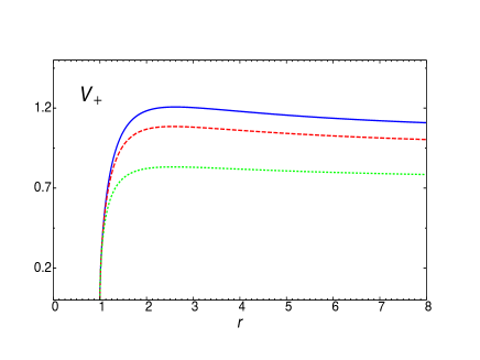
in which $V(r)$ is the effective potential for the scalar field dynamics in the black hole geometry. Explicitly, we have

$$V(r)=f(r)\left(\frac{m^{2}}{r^{2}}-\frac{f(r)}{4r^{2}}+\frac{1}{2r}\frac{df(r)}{dr}\right).$$ (18)

The effective potential $V(r)$ depends on all the parameters that characterize the black hole geometry $(M,L,\alpha)$ and on the scalar field azimutal number $m$.

In Fig. 2 we plot different potentials varying the GB parameter $\alpha$ with fixed $M$, $L$, and $m$. For $\alpha=0$ we recover the effective potential for the BTZ black hole Cardoso and Lemos (2001) and as $\alpha$ increases, the value of the potential for a given radial position $r$ decreases, showing that the GB coupling attenuates the interaction between the geometry and the probe massless scalar field.

Figure 2: (color online) Main panel: Effective scalar potential $V(r)$ with $m=0$, $M=L=1$ for different values of GB coupling $\alpha=0$ (blue), $\alpha=5\times 10^{-2}$ (dashed red), and $\alpha=3\times 10^{-1}$ (dotted green). Upper left panel: Effective scalar potential $V(r)$ with $m=2$, $M=L=1$ for different values of GB coupling $\alpha=0$ (blue), $\alpha=5\times 10^{-2}$ (dashed red), and $\alpha=3\times 10^{-1}$ (dotted green).

The quasinormal spectra due to the evolution of a massless scalar field can be obtained with several known methods. We consider the characteristic integration in double null coordinates given by $du=dt-dr_{*}$ and $dv=dt+dr_{*}$, turning Eq. (17) to the form

$$\left(4\frac{\partial^{2}}{\partial u\partial v}+V(r)\right)\psi=0.$$ (19)

Now, the usual discretization scheme (described in the specific literature Konoplya and Zhidenko (2011) and references therein) gives the following equation,

$$\psi_{N}=\left(1+\frac{h^{2}}{16}V_{S}\right)^{-1}\left(\psi_{W}+\psi_{E}-\psi_{S}-\frac{h^{2}}{16}(V_{W}\psi_{W}+V_{E}\psi_{E}+V_{S}\psi_{S})\right)\,,$$ (20)

which we can integrate yielding the field evolution with the quasinormal signal present. After getting the field profile, acquired through the characteristic integration, we can apply the Prony method described in Konoplya and Zhidenko (2011) to pick up the frequencies.

In order to cross-check the results of the obtained quasinormal modes, we also developed a Frobenius method, similar to that of Ref. Horowitz and Hubeny (2000). The equations for this numerical implementation are given in Appendix A. We obtained a good agreement between the results collected with both methods for $\alpha<0.13$. The maximum deviation between the results of both methods appears in the case of very small $\alpha$. Actually, for $\alpha=10^{-4}$ we obtained an outcome with a $2\%$ maximal deviation in the cases of higher $r_{+}$. Except for those occurrences, the convergence of both methods is higher than $0.2\%$. The Tables 1 and 2 display the quasinormal frequencies for different geometry parameters.

Table 1: The fundamental quasinormal modes for a massless scalar field with $L=1$ and azimutal number $m=0$.

	$r_{+}=1$		$r_{+}=10$		$r_{+}=100$
$\alpha$	$\Re(\omega)$	$-\Im(\omega)$	$\Re(\omega)$	$-\Im(\omega)$	$\Re(\omega)$	$-\Im(\omega)$
$1\cdot 10^{-4}$	0.0201015	1.99975	0.204054	19.99609	2.04054	199.96092
$1\cdot 10^{-3}$	0.0633286	1.99781	0.633286	19.97806	6.33286	199.78061
$1\cdot 10^{-2}$	0.198807	1.97948	1.98807	19.79481	19.88068	197.94808
$1\cdot 10^{-1}$	0.572319	1.79642	5.72319	17.96419	57.23187	179.64185
$2\cdot 10^{-1}$	0.718720	1.62834	7.18720	16.28342	71.87195	162.83424
$3\cdot 10^{-1}$	0.788886	1.49642	7.88886	14.96417	78.88860	149.64175
$4\cdot 10^{-1}$	0.825547	1.39082	8.25547	13.90820	82.55466	139.08200
$5\cdot 10^{-1}$	0.844776	1.30425	8.44776	13.04249	84.47757	130.42490

Table 2: The fundamental quasinormal modes for a massless scalar field with $L=1$ and azimutal number $m=1$.

	$r_{+}=1$		$r_{+}=10$		$r_{+}=100$
$\alpha$	$\Re(\omega)$	$-\Im(\omega)$	$\Re(\omega)$	$-\Im(\omega)$	$\Re(\omega)$	$-\Im(\omega)$
$1\cdot 10^{-4}$	0.999652	1.99883	1.02051	19.99608	2.27236	199.96092
$1\cdot 10^{-3}$	1.00185	1.99727	1.18394	19.97796	6.41138	199.78060
$1\cdot 10^{-2}$	1.01893	1.97500	2.22700	19.79394	19.90599	197.94799
$1\cdot 10^{-1}$	1.13028	1.77622	5.80817	17.96072	57.24044	179.64150
$2\cdot 10^{-1}$	1.18365	1.60429	7.25065	16.27948	71.87833	162.83384
$3\cdot 10^{-1}$	1.20435	1.47060	7.94319	14.96002	78.89406	149.64133
$4\cdot 10^{-1}$	1.20937	1.36369	8.30458	13.90386	82.55958	139.08156
$5\cdot 10^{-1}$	1.20626	1.27595	8.49345	13.03798	84.48215	130.42445

The fundamental frequencies with $m=0$ show an interesting feature: there is a linear scaling between the real and imaginary parts of $\omega$ and the black hole event horizon, a characteristic first observed in Horowitz and Hubeny (2000). In that work the temperature and the quasinormal modes are fitted by a straight line for large black holes (high $r_{+}$) in AdS universes. However, for intermediate size black holes (with size of the order of the AdS radius) this scaling disappears. One of the reasons put forward by the authors is that when the temperature is slowly lowered, one encounters the Hawking-Page transition and the supergravity description is no longer valid, i.e., the relaxation time is not related to the imaginary part of the fundamental quasinormal frequency anymore. In our case we still preserve the scaling with the temperature even for intermediate size black holes since the relation $T\propto r_{+}$ is always valid. Thus, using the same argument given in Ref. Horowitz and Hubeny (2000) we can conclude that this scaling is kept because there are no phase transitions in the (2+1)-dimensional GB-BTZ black hole, a fact that we will briefly discuss in Sec. VI.

Figure 3: Quasinormal modes of the GB-BTZ black hole for different coupling parameter. The azimutal number of the field reads $m=0$.

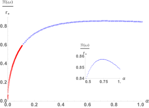
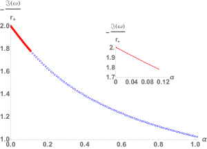
In Fig. 3 we show the quasinormal modes for different values of $\alpha$ parameter. The interesting feature here is the increment of the value of $\Re(\omega)$ with increasing $\alpha$, together with the attenuation of $-\Im(\omega)$. In the small-$\alpha$ regime ($m=0$) our results for the real part of the frequency suggest a scaling given by

$$\Re(\omega)=(0.843-0.738e^{-10.663\alpha})r_{+}\,,$$ (21)

and a linear scaling for the imaginary part expressed by

$$-\Im(\omega)=(1.9999-2.0435\alpha)r_{+}\,,$$ (22)

with linear correlation factor $R^{2}=0.99976$.

In Fig. 3, we observe that the real part of the quasinormal frequencies increases with $\alpha$, reaching a maximum at $\alpha=\alpha_{max}$ and then starts to decrease. The same behavior was obtained in the case of massless scalar perturbations of the $(3+1)$-dimensional GB black hole Konoplya and Zinhailo (2020), where the value $\alpha=\alpha_{max}$ indicates the possibility of gravitational instabilities since $\Re(\omega)$ is non-monotonic.

Since no negative potential was present in the region I of the Penrose diagram for every tested parameter, we consistently found no instabilities in the propagation of the scalar field subject to well-behaved initial data. Thus, the scalar perturbation can be decomposed after an initial burst in the traditional towers of quasinormal modes labeled by an overtone number. Whether more than one family of quasinormal modes can exist in the (2+1)-dimensional GB-BTZ black hole geometry remains an open issue to be further investigated.

In the next section we follow our stability study with the Weyl field, whose perturbative analysis is also performed with the same tools described in the present section.

IV Probe massless spinorial field

In this section we are going to consider the problem of a massless spinor field $\Phi$ evolving in the geometry of the (2+1)-dimensional GB-BTZ black hole (5). The equation that dictates the dynamics of $\Phi$ is the well-known Dirac equation in its covariant form,

$$i\gamma^{(a)}e_{(a)}^{\;\mu}\nabla_{\mu}\Phi=0,$$ (23)

where our index notation is the following, Latin indices enclosed in parenthesis refer to the coordinates defined in the flat tangent space and Greek indices indicate the spacetime coordinates. In the tangent space we define the triad basis as in Eq. (84) and the spinor covariant derivative $\nabla_{\mu}$ is given by the following expression,

$$\nabla_{\mu}=\partial_{\mu}+\frac{1}{8}\omega^{(a)(b)}\left[\gamma_{(a)},\gamma_{(b)}\right],$$ (24)

in terms of spin connections $\omega_{\mu}^{(a)(b)}$ and gamma matrices $\gamma^{(a)}$, which can be written in terms of usual Pauli matrices . The components of the spin connection can be computed using the expression in terms of the triad and the spacetime metric connections $\Gamma_{\mu\rho}^{\nu}$ as

$$\omega_{\mu}^{(a)(b)}=e_{\nu}^{(a)}\partial_{\mu}e^{(b)\nu}+e_{\nu}^{(a)}\Gamma^{\nu}_{\mu\rho}e^{\rho(b)}.$$ (25)

The explicit expressions for the triad basis and the metric connections are given in Appendix B. Here we list the two non-vanishing components of $\omega_{\mu}^{(a)(b)}$, computed using the expressions (84)-(B),

$$\omega_{t}^{(t)(r)}=\frac{1}{2}\frac{df}{dr}\,,\quad\omega_{\varphi}^{(r)(\varphi)}=-\sqrt{f}.$$ (26)

The spinor field $\Phi$ can be written in terms of its two-components $\Phi_{1}$ and $\Phi_{2}$ as

$$\Phi=\begin{pmatrix}\Phi_{1}(t,r,\varphi)&\\ \Phi_{2}(t,r,\varphi)&\\ \end{pmatrix}.$$ (27)

Using the tortoise coordinate $r_{*}$ and redefining the spinor components as

$$\begin{pmatrix}\Phi_{1}(t,r,\varphi)&\\ \Phi_{2}(t,r,\varphi)&\\ \end{pmatrix}=\begin{pmatrix}i\left(r^{2}f\right)^{1/4}e^{-i\omega t+im\varphi}Y_{+}(r)&\\ \left(r^{2}f\right)^{1/4}e^{-i\omega t+im\varphi}Y_{-}(r)&\\ \end{pmatrix},$$ (28)

the Dirac equation (23) can be cast to the following form

$$\left(\frac{d}{dr_{*}}\pm i\omega\right)Y_{\pm}=WY_{\mp},$$ (29)

where the superpotential $W$ is given by

$$W=m\frac{\sqrt{f}}{r}.$$ (30)

Figure 4: Left panel: Potential $V_{+}$ for the massless spinor with $\alpha=0$ (blue), $\alpha=0.1$ (dashed red), and $\alpha=0.5$ (dotted green). Right panel: Potential $V_{-}$ for the massless spinor with the same values of $\alpha$ as in the left panel.

The final step to obtain the so-called superpartner potentials $V_{\pm}$ is to introduce the pair of coordinates $R_{+}$ and $R_{-}$ as $R_{\pm}=Y_{+}\pm Y_{-}$ into (29), so that

$$\left(\frac{d^{2}}{dr_{*}^{2}}+\omega^{2}\right)R_{\pm}=V_{\pm}R_{\pm}\,,$$ (31)

where $V_{\pm}$ can be expressed in terms of the superpotential $W$ as

$$V_{\pm}=W^{2}\pm\frac{dW}{dr_{*}}\,.$$ (32)

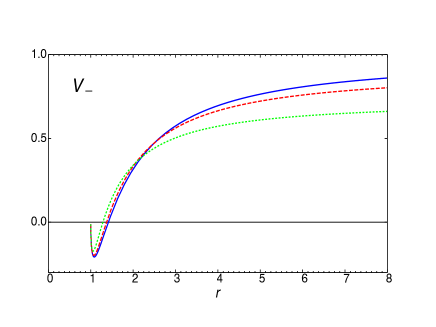
Finally, the explicit form of the superpartner potentials for the massless spinorial field evolving in the spacetime of the (2+1)-dimensional GB-BTZ black hole is

$$V_{\pm}=m^{2}\frac{f}{r^{2}}\pm m\frac{\sqrt{f}}{r}\left[\frac{1}{2}\frac{df}{dr}-\frac{f}{r}\right].$$ (33)

The propagation of a massless spinor field in the black hole geometry dictated by Eq. (31) recovers the quasinormal modes through the signal of field profiles. The profiles are obtained as described in the previous section with the double null integration technique. After an initial perturbation (gauge), the quasinormal evolution takes place and the frequencies are drawn with the Prony method, mentioned in the previous section. We use the usual gaussian packages in null coordinates as initial surface to evolve the field.

Table 3: The fundamental quasinormal modes for a massless spinorial field with $L=1$ and azimutal number $m=1$ with potential $V_{+}$. The frequencies represent a stable field evolution with a purely imaginary decay, except for $r_{+}=1$.

$r_{+}$	$\alpha$
	0.001	0.01	0.1	0.2	0.3	0.4	0.5
1	1.10795	1.10722	1.09530	1.07726	1.05788	1.03867	1.02019
	-0.86224i	-0.85258i	-0.76950i	-0.69847i	-0.64240i	-0.59673i	-0.55863i
5	-2.71475i	-2.71715i	-2.74155i	-2.77000i	-2.80042i	-2.83343i	-2.86972i
10	-5.10072i	-5.10171i	-5.11161i	-5.12270i	-5.13402i	-5.14566i	-5.15771i
50	-25.01925i	-25.01943i	-25.02117i	-25.02308i	-25.02501i	-25.02695i	-25.02893i
100	-50.00967i	-50.00976i	-50.01062i	-50.01158i	-50.01253i	-50.01350i	-50.01448i

Table 4: The fundamental quasinormal modes for a massless spinorial field with $L=1$ and azimutal number $m=1$ with potential $V_{-}$. The frequencies represent a stable field evolution with a purely imaginary decay.

$r_{+}$	$\alpha$
	0.001	0.01	0.1	0.2	0.3	0.4	0.5
1	-0.10731i	-0.10670i	-0.10115i	-0.095998i	-0.091609i	-0.087790i	-0.084415i
5	-2.33789i	-2.33677i	-2.32594i	-2.31449i	-2.30348i	-2.29281i	-2.28241i
10	-4.91111i	-4.91040i	-4.90340i	-4.89582i	-4.88837i	-4.88098i	-4.87362i
50	-24.98117i	-24.98100i	-24.97936i	-24.97756i	-24.97576i	-24.97395i	-24.97211i
100	-49.99043i	-49.99035i	-49.98951i	-49.98858i	-49.98766i	-49.98673i	-49.98579i

The quasinormal modes are listed in the Tables 3 and 4. There we can verify an interesting behavior: for increasing $\alpha$ the damping factor varies in opposite directions, increasing for $V_{+}$ and decreasing for $V_{-}$. This effect is more pronounced for small $r_{+}$ such that the spectra of larger black holes are very mildly influenced by the variation of $\alpha$. A scaling between $r_{+}$ and the quasinormal frequency emerges for large black holes,

$$\omega\simeq\frac{r_{+}}{2}$$ (34)

for both $V_{+}$ and $V_{-}$. This is the same result obtained for the quasinormal modes of the BTZ black hole to zeroth order in $m$ de Oliveira and Fontana (2018). Interestingly, $\alpha$ plays no important role in the spectra for large black holes in the spinorial field profile contrarily to the scalar case.

The evolution of the massless spinorial field was extensively investigated with our methods and found to be stable. The field profile, after an initial burst, decomposes into a tower of quasinormal modes from which specific cases are listed in Tables 3 and 4. This is an expected result for the potential $V_{+}$, however, it is not granted for the potential $V_{-}$ since a small region with $V<0$ exists for $r>r_{+}$ in this case.

As usual, in AdS-like black holes the spectra for both $V_{+}$ and $V_{-}$ are not the same. Such behavior of isospectrality of the potentials is found whenever a series expansion of the transmission coefficients associated to $W$ is the same for $V_{+}$ and $V_{-}$ Chandrasekhar (1985); Cardoso (2004). The fact that

$$W\Big{|}_{r\rightarrow r_{+}}^{r\rightarrow\infty}=W_{\infty}>0\,.$$ (35)

is sufficient to break the isospectrality of the potentials.

V Scalar quasinormal modes in the hydrodynamical approximation

In this section we are going to consider the hydrodynamical limit of probe scalar field. In general, an interacting theory can be described by means of hydrodynamics in the limit of large wavelength and small wavenumbers compared to the typical temperature of the system Landau and Lifshitz (1987). From Gauge/Gravity correspondence it is well-know that the characteristic thermalization timescale for a dual thermal state at the boundary is given by the inverse of the imaginary part of the fundamental quasinormal frequency in the hydrodynamical limit Horowitz and Hubeny (2000). Such a result has been confirmed in $(2+1)-$dimensional black holes with Lifshitz scaling Abdalla et al. (2012).

In order to establish this limit, we define the quantities $\mathfrak{w}=\omega/2\pi T$ and $\mathfrak{q}=m/2\pi T$ and consider the limit $\mathfrak{q}\rightarrow 0$, such that the radial equation for the massless scalar field can be cast to

$$R^{\prime\prime}(u)+\left[\frac{h^{\prime}}{h}-\frac{1}{u}\right]R^{\prime}(u)+\frac{4\alpha^{2}}{h^{2}L^{4}}\mathfrak{w}^{2}R(u)=0,$$ (36)

where we have performed the change of variable $u=r_{+}/r$ and defined

$$h=1-\left[1+\frac{4\alpha}{L^{2}}(1-u^{2})\right]^{1/2}.$$ (37)

In the case in which $\mathfrak{w}<<1$ we expand $R(u)$ in powers of $\mathfrak{w}$,

$$R(u)\approx h(u)^{\sigma}\left(F_{0}(u)+i\mathfrak{w}F_{1}(u)+\mathcal{O}(\mathfrak{w}^{2})\right).$$ (38)

The exponent $\sigma$ is determined by imposing the ingoing boundary condition for the scalar field at the location of the black hole event horizon $r_{+}$. We thus obtain $\sigma=-i\mathfrak{w}/2$.

Substituting the expansion (38) in the scalar field radial equation (36) we obtain two ordinary differential equations for the functions $F_{0}(u)$ and $F_{1}(u)$,

$$F_{0}^{\prime\prime}(u)+\left(\frac{h^{\prime}}{h}-\frac{1}{u}\right)F_{0}^{\prime}(u)=0\,,$$ (39)

$$F_{1}^{\prime\prime}(u)+\left(\frac{h^{\prime}}{h}-\frac{1}{u}\right)F_{1}^{\prime}(u)-\frac{h^{\prime}}{h}F_{0}^{\prime}+\left(\frac{h^{\prime}}{u}-h^{\prime\prime}\right)\frac{F_{0}}{2h}=0\,.$$ (40)

In order to analyze the influence of GB coupling constant $\alpha$ on the frequencies in the hydrodynamical limit, we will consider the small-$\alpha$ limit. Expanding $h(u)$ in such a limit we obtain,

$$h(u)\approx\frac{2}{L^{2}}(u^{2}-1)\left[\alpha+\frac{\alpha^{2}}{L^{2}}(u^{2}-1)\right]\,.$$ (41)

In this scenario the solution for Eq. (39) is

$$F_{0}(u)=A-\frac{B}{2L^{2}}\ln\left[{\frac{(u^{2}-1)}{(L^{2}+\alpha(u^{2}-1))}}\right]\,,$$ (42)

where $A$ and $B$ are constants. To satisfy the ingoing boundary condition at the event horizon and avoid divergences in $F_{0}(u)$, we need impose $B=0$ in (42). Thus, the solution becomes $F_{0}(u)=A$. With this result we solve Eq. (40) for $F_{1}(u)$ obtaining,

$$F_{1}(u)=C+\frac{2A\alpha-D}{2L^{2}}\ln{(u^{2}-1)}+\frac{D+2A(L^{2}-\alpha)}{2L^{2}}\ln{[L^{2}+(u^{2}-1)\alpha]},$$ (43)

where $C$ and $D$ are constants. Again, the solution has to be finite as $u\rightarrow 1$, thus, we must have $D=2A\alpha$. Also, the ingoing boundary condition at the event horizon implies that $F_{1}(1)=0$, then,

$$C=-A\ln{(L^{2})}.$$ (44)

Finally, the solution for $F_{1}(u)$, finite and obeying the physical boundary condition at the event horizon, turns to be

$$F_{1}(u)=A\ln{\left[1+\frac{\alpha}{L^{2}}(u^{2}-1)\right]}.$$ (45)

Replacing the solutions for $F_{0}(u)$ and $F_{1}(u)$ back in Eq. (38) we have

$$R(u)=A\,h(u)^{-i\mathfrak{w}/2}\left\{1+i\mathfrak{w}\ln{\left[1+\frac{\alpha}{L^{2}}(u^{2}-1)\right]}\right\}\,.$$ (46)

Imposing the Dirichlet boundary condition at spatial infinity for the scalar field, $R(0)=0$, we arrive to the following allowed set of frequencies,

$$\mathfrak{w}=\frac{i}{\ln{\left(1-\frac{\alpha}{L^{2}}\right)}},$$ (47)

which in terms of black hole temperature $T$ reads

$$\omega=\frac{2\pi Ti}{\ln{\left(1-\frac{\alpha}{L^{2}}\right)}}.$$ (48)

The hydrodynamical frequencies are purely imaginary, showing the same behavior as the three-dimensional black holes with Lifshitz symmetry Abdalla et al. (2012) and those surrounded by anisotropic fluids de Oliveira and Fontana (2018). In terms of Gauge/Gravity correspondence the perturbation of a black hole in the gravity side is equivalent to perturb a thermal state in the gauge theory side. In this context, the inverse of the imaginary part of the fundamental quasinormal frequency corresponds to the relaxation time which the perturbed thermal state needs in order to return to thermal equilibrium. Thus, in our case this timescale is given by

$$\tau=\frac{\ln{\left(1-\frac{\alpha}{L^{2}}\right)}}{2\pi T}.$$ (49)

At high temperatures the timescale $\tau$ approaches zero suggesting that the perturbations of thermal states in the $(1+1)-$field theory are not long-lived. However, as $\alpha$ increases (provided that $-L^{2}/4<\alpha<0$) with fixed black hole temperature, the timescale $\tau$ increases as well indicating the possibility of having long-lived perturbations in the gauge theory.

In the next section we will discuss some aspects of the thermodynamics of (2+1)-dimensional GB-BTZ black holes.

VI Thermodynamical aspects

The thermodynamics of the black hole described by the negative branch of Eq. (5) is very simple as quoted by Hennigar et al. (2020a), in which the main thermodynamical variables are listed as follows,

$$T=\frac{r_{+}}{2\pi L^{2}}\,,\quad P=\frac{1}{8\pi L^{2}}\,,\quad V=\pi r_{+}^{2}\,,$$

$$M=\frac{r_{+}^{2}}{8L^{2}}\,,\quad S=\frac{\pi r_{+}}{2}\,,\psi_{\alpha}=0\,,$$ (50)

where $\psi_{\alpha}$ is the potential conjugated to the GB parameter. In particular, we notice that its Hawking temperature grows monotonically with $r_{+}$, so that there are no phase transitions. This fact can also be seen from the simple equation of state obtained combining $T$, $V$, and $P$ in the list of Eqs.(VI),

$$P=\frac{T}{v}\,,$$ (51)

where we have defined the specific volume as ${v}=4\sqrt{V/\pi}$. This equation clearly has no critical points.

Another analysis that supports this conclusion is the study of null geodesics in this geometry. It is known that the photon sphere radius and the impact parameter related to it play an interesting role during a black hole phase transition and can serve as order parameters to describe such a phenomenon Wei and Liu (2018). Thus, by considering the Lagrangian

$$2{\cal L}=-f(r)\dot{t}^{2}+\frac{\dot{r}^{2}}{f(r)}+r^{2}\dot{\varphi}^{2}\,,$$ (52)

and the constants of motion defined by the generalized momenta corresponding to $t$ and $\varphi$,

$$p_{t}=-f(r)\dot{t}=-E\,,\qquad p_{\varphi}=r^{2}\dot{\varphi}=L\,,$$ (53)

we can obtain the radial equation for a photon moving in this spacetime,

$$\dot{r}^{2}+V_{eff}=0\,,\quad\hbox{with }\quad V_{eff}=\frac{fL^{2}}{r^{2}}-E^{2}\,.$$ (54)

Applying the usual conditions in order to obtain the photon sphere radius $r_{ps}$

$$V_{eff}=0\,,\quad\frac{dV_{eff}}{dr}=0\,,\quad\frac{d^{2}V_{eff}}{dr^{2}}<0\quad\hbox{at }r_{ps}\,,$$ (55)

we notice that the second equation of set (55) cannot be solved for any finite $r_{ps}$. In fact, as happens in BTZ solution, this (2+1)-dimensional GB-BTZ black hole has no photon circumference. Then, the absence of phase transitions becomes evident.

In what follows we discuss some entropy aspects for this geometry, namely, we calculate the Bekenstein entropy bound and the leading correction to the black hole entropy using the brickwall method.

VI.1 Entropy bound

We consider the motion of a particle near a black hole described by the metric (5). The constants of motion correspond to the energy and angular momentum of the particle, respectively,

$$E = \pi_{t}=g_{tt}\dot{t}\,,$$

$$J = -\pi_{\varphi}=-g_{\varphi\varphi}\dot{\varphi}\,.$$ (56)

In addition, the energy conservation for a particle of mass $m$ implies,

$$-m^{2}=g^{\mu\nu}\pi_{\mu}\pi_{\nu}\,,$$ (57)

so that

$$r^{2}E^{2}-J^{2}f(r)-m^{2}r^{2}f(r)=0\,,$$ (58)

whose solution gives an expression for the particle’s energy,

$$E=\frac{\sqrt{f(r)}}{r}\sqrt{J^{2}+m^{2}r^{2}}\,.$$ (59)

As the particle is gradually approaching the black hole, it finally reaches the event horizon when the proper distance from its center of mass to this horizon equals $R$, the characteristic dimension of the particle,

$$\int_{r_{+}}^{r_{+}+\delta(R)}\sqrt{g_{rr}}dr=R\,,$$ (60)

where the upper limit of the integral represents the point of capture of the particle by the black hole. Expanding to first order we obtain for $\delta$,

$$\delta(R)\approx\frac{r_{+}R^{2}}{2L^{2}}\,.$$ (61)

And we can minimize the energy (59) at the point of capture with respect to the particle’s angular momentum, i.e.,

$$\frac{dE}{dJ}\bigg{|}_{r_{+}+\delta}=0\quad\Rightarrow\quad J=0\,,$$ (62)

thus obtaining,

$$E_{min}=m\sqrt{f(r_{+}+\delta)}=\frac{mr_{+}R}{L^{2}}\,.$$ (63)

Now, according to the first law of thermodynamics we have that

$$dM=E_{min}=T\,dS=\frac{\kappa}{2\pi}dS\,,$$ (64)

being $\kappa$ the surface gravity at the event horizon,

$$\kappa=\frac{f^{\prime}}{2}\bigg{|}_{r=r_{+}}=\frac{r_{+}}{L^{2}}\,.$$ (65)

At the same time, the generalized second law of thermodynamics says that after the capture of the particle the entropy of the black hole cannot decrease,

$$S_{BH}(M+dM)\geq S_{BH}(M)+S\,.$$ (66)

Thus, combining both laws we can obtain an upper bound on the entropy of the particle

$$S\leq dS=S_{BH}(M+dM)-S_{BH}(M)=2\pi mR\equiv 2\pi ER\,.$$ (67)

This bound shows to be independent of the black hole parameters and agrees with the universal result obtained by Bekenstein Bekenstein (1981), valid for any dimensionality.

VI.2 Entropy semiclassical correction

In order to find semiclassical corrections to the black hole entropy, we use ’t Hooft’s brickwall method ’t Hooft (1985). This method considers a thermal bath of scalar fields quantized using the partition function of statistical mechanics, whose leading contribution yields the Bekenstein-Hawking formula. The method introduces certain conditions on the scalar field $\Phi$ aiming to avoid divergences, namely, an ultraviolet cut-off near the event horizon ($\Phi=0$ for $r\leq r_{+}+\epsilon$) and an infrared cut-off far from the black hole ($\Phi=0$ for $r\geq L\gg r_{+}$).

The scalar field of mass $\mu$ obeys the massive version of the Klein-Gordon equation given by Eq. (15),

$$\frac{1}{\sqrt{-g}}\partial_{\mu}(\sqrt{-g}g^{\mu\nu}\partial_{\nu}\Phi)-\mu^{2}\Phi=0\,.$$ (68)

Using the ansatz $\Phi(t,r,\varphi)=e^{-iEt+im\varphi}R(r)$ the radial part of Eq. (68) turns out to be

$$\frac{d^{2}R}{dr^{2}}+\left(\frac{f^{\prime}}{f}+\frac{1}{r}\right)\frac{dR}{dr}+\frac{1}{f}\left(\frac{E^{2}}{f}-\frac{m^{2}}{r^{2}}-\mu^{2}\right)R=0\,.$$ (69)

In order to obtain the radial wave number $K$, we use a WKB approximation for $R(r)\sim e^{iS(r)}$, with $S(r)$ being a rapidly varying phase. To leading order the only significative contribution to the radial wave number comes from the first derivative of $S$ obtained from the real part of Eq. (69),

$$K\equiv S^{\prime}=\frac{1}{\sqrt{f}}\left[\frac{E^{2}}{f}-\left(\frac{m^{2}}{r^{2}}+\mu^{2}\right)\right]^{1/2}\,.$$ (70)

Then, we use $K$ to quantize the number of radial modes $n_{r}$ of the field as follows,

$$\pi n_{r}=\int_{r_{+}+\epsilon}^{L}K(r,m,E)\,dr\,.$$ (71)

Moreover, in order to find the black hole entropy of the system, we calculate the Helmholtz free energy $F$ of the scalar thermal bath with temperature $\beta^{-1}=\kappa/2\pi$ as follows,

$$F=\frac{1}{\beta}\int 2\,dm\int\ln(1-e^{-\beta E})\,dn_{r}=-\int 2\,dm\int\frac{n_{r}}{e^{\beta E}-1}\,dE\,.$$ (72)

Performing the integral in $m$ and using Eq. (71) we obtain

$$F=-\frac{1}{2}\int_{0}^{\infty}\frac{dE}{e^{\beta E}-1}\int_{1+\bar{\epsilon}}^{\bar{L}}\frac{r_{+}^{2}y}{\sqrt{f(y)}}\left(\frac{E^{2}}{f(y)}-\mu^{2}\right)dy\,,$$ (73)

where we rescaled the quantities, $y=r/r_{+}$, $\bar{L}=L/r_{+}$, and $\bar{\epsilon}=\epsilon/r_{+}$. Thus, the metric coefficient can be written as

$$f(y)=-\frac{r_{+}^{2}}{2\alpha}y^{2}\left[1-\sqrt{1+\frac{4\alpha}{y^{2}L^{2}}(y^{2}-1)}\right]\,.$$ (74)

Expanding near the event horizon where $y\rightarrow 1$ and performing the Bose-Einstein integral we get

$$F\approx-\frac{\zeta(3)}{\beta^{3}}\frac{(2\alpha)^{3/2}}{r_{+}}\int_{1+\bar{\epsilon}}^{\bar{L}}\left[-1+\sqrt{1+\frac{4\alpha}{L^{2}}(y^{2}-1)}\right]^{-3/2}dy\,,$$ (75)

with $\zeta(x)$ being the Riemann zeta function. The semiclassical correction we are searching comes from the divergent contribution of Eq. (75), i.e., from the lower limit of the integral, whose leading order term reads,

$$F_{\epsilon}=-\frac{\zeta(3)L^{3}}{\beta^{3}\sqrt{2r_{+}\epsilon}}\,.$$ (76)

The corresponding entropy $S_{\epsilon}$ follows directly,

$$S_{\epsilon}=\beta^{2}\frac{\partial F_{\epsilon}}{\partial\beta}=\frac{3\zeta(3)L^{3}}{\beta^{2}\sqrt{2r_{+}\epsilon}}\,.$$ (77)

In order to write this correction in a more familiar way, we use the proper thickness $\xi$ defined as

$$\xi=\int_{r_{+}}^{r_{+}+\epsilon}\sqrt{g_{rr}}\,dr\approx\frac{L\sqrt{2\epsilon}}{\sqrt{r_{+}}}\,,$$ (78)

as well as the event horizon “area” $A=2\pi r_{+}$ and the Hawking temperature $T=\frac{1}{\beta}=\frac{r_{+}}{2\pi L^{2}}$, obtained from the surface gravity (65), to finally achieve,

$$S_{\epsilon}=\frac{3\zeta(3)A}{8\pi^{3}\xi}\,,$$ (79)

which is a universal expression in three-dimensional gravity Kim et al. (2006); Kim and Son (2009).

VII Final Remarks

In this paper, we have studied the perturbative and thermodynamical aspects of the $(2+1)$-dimensional GB-BTZ black hole found by Hennigar et. al. Hennigar et al. (2020a, 2021). This solution describes a family of lower-dimensional black holes parametrized by the mass term $M$, the AdS₃ radius $L$, and the GB coupling constant $\alpha$. Also, the BTZ limit of the solutions exists as $\alpha\rightarrow 0$, and the event horizon is located at $r_{+}=LM^{1/2}$. In order to understand the role of the GB coupling constant $\alpha$ in the context of the black hole stability problem, we performed the computations and analysis of the GB-BTZ black hole quasinormal spectrum. In addition, the Bekenstein entropy bound and the semiclassical correction to the Bekenstein-Hawking entropy were also computed.

We analyzed two different types of perturbations represented by a scalar field and a massless spinorial field. For intermediate black holes, both scalar and spinorial perturbations are affected reasonably by the variation of the GB coupling constant, although the influence in the scalar case is much more pronounced. This is also true for large black holes perturbed by the scalar field. Interestingly enough, such a picture changes for large black holes in the massless spinorial case, where the influence of the coupling constant is almost insignificant. To first order in the angular momentum we can understand the perturbation in a common ground as the same reported for a BTZ black hole when $\alpha=0$ (see e. g. de Oliveira and Fontana (2018)), establishing no role played by $\alpha$ on the perturbation. In both cases analyzed here the extensive search for profiles with different geometry parameters results in a stable spacetime against the field perturbations.

The quasinormal modes obtained for the scalar and spinorial perturbations in the background of the GB-BTZ black hole are assembled in Tables 1 to 4 and display interesting features of the geometry, already described in the previous sections. In the scalar case, for instance, we remark the presence of a peak in the graphic of $\frac{\Re(\omega)}{r_{+}}$ vs. $\alpha$ and the linear scaling of $\alpha$ and $-\frac{\Im(\omega)}{r_{+}}$ in the small-$\alpha$ regime. Moreover, for the fundamental mode we see a linear scaling between the quasinormal frequencies and the temperature of the black hole, which can be interpreted as an absence of phase transitions in the model, also confirmed by the thermodynamical analysis.

As for the massless spinorial perturbation, only oscillatory modes are present for the scalar field with $V_{-}$ potential, different from what is found in the pure BTZ case Cardoso and Lemos (2001) and the (2+1)-dimensional Lifshitz black hole Cuadros-Melgar et al. (2012). In the case of $V_{+}$ potential a critical $r_{+}$ exists such that it points out the transition from oscillatory to non-oscillatory modes, a behavior also found in $(2+1)$-dimensional-black holes with anisotropic fluids de Oliveira and Fontana (2018).

Subsequently, regarding the quasinormal spectrum due to scalar perturbations, we found that the hydrodynamical or high-temperature approximation leads to an exact result for the quasinormal spectrum $w=i(2\pi T)/\ln(1-\alpha/L^{2})$ in the small-$\alpha$ limit provided that $-L^{2}/4<\alpha<0$. As the hydrodynamical frequencies are purely imaginary, there is not oscillatory phase in this limit either. In the context of Gauge/Gravity correspondence this result suggests that perturbations of thermal states in the $(1+1)-$field theory are not long-lived.

Afterwards, we briefly discussed the thermodynamics of the (2+1)-dimensional GB-BTZ black hole, stressing that there are no phase transitions since its temperature is a monotonic growing function, a result that is also reinforced by the absence of a photon circumference in the geometry. Furthermore, we calculated the Bekenstein entropy bound for an object captured by this black hole obeying the first and second laws of thermodynamics. Our result complies with the universality of the bound. In addition, we computed the leading semiclassical correction to the Bekenstein-Hawking entropy by means of the brickwall method. This correction shows a perfect agreement with other (2+1)-dimensional black holes.

Finally, according to our results we can conclude that the (2+1)-dimensional GB-BTZ black holes are dynamically stable under scalar and spinorial linear perturbations. We should also stress that as in this dimensionality the metric or gravitational perturbations reduce to a scalar mode only because there are no propagating degrees of freedom Carlip (2005), what also happens even in higher-dimensional braneworld models Cuadros-Melgar et al. (2011), our stability analysis is a good candidate for a definitive answer on this matter. Moreover, this dynamical stability is also accompanied by a thermodynamical stability and a full agreement of our results with the universality of entropy aspects discussed here. The stability analysis of more general solutions, including charge or angular momentum as shown in Ref.Hennigar et al. (2020c), is left for future works.

Appendix A Frobenius method for the Klein-Gordon equation

The Frobenius method we developed for the scalar field propagation starts by taking Eq. (17) and defining a new variable $x=r^{-1}$. In such coordinates the field equation reads

$$s\psi^{\prime\prime}+\tau\psi^{\prime}+u\psi=0\,,$$ (80)

in which prime denotes a derivative with respect to $x$ and the functions $s$, $\tau$, and $u$ are given by

$$s=f^{2}x^{4}\equiv\sum_{n=0}^{\infty}s_{n}(x-x_{+})^{n+\delta}\,,$$

$$\tau=fx^{2}(2xf+x^{2}f^{\prime})\equiv\sum_{n=0}^{\infty}\tau_{n}(x-x_{+})^{n+\delta}\,,$$

$$u=\omega^{2}-V\equiv\sum_{n=0}^{\infty}u_{n}(x-x_{+})^{n+\delta}\,.$$ (81)

Now, using the Ansatz $\psi=\sum a_{n}(x-x_{+})^{n+\delta}$ the solution to leading order (indicial relation) is given by the expression,

$$\delta=\pm i\frac{\omega r_{+}}{2M}\,,$$ (82)

being the negative sign the correct one according to the right boundary condition. Substituting the ansatz in the field equation we still retain the recurrence relation,

$$a_{n}=-\frac{1}{D_{n}}\sum_{k=0}^{n-1}\{s_{n-k+2}[k(k-1)+\delta(2k-1)+\delta^{2}]+\tau_{n-k+1}[k+\delta]+u_{n-k}\}a_{k}$$ (83)

with $D_{n}=n(n+2\delta)s_{2}$. Such a expression allows us to solve the quasinormal problem in a similar way as that described in Horowitz and Hubeny (2000).

Appendix B Metric connections and triad basis

The components of triad basis for the metric (5) are given by

$$e_{t}^{(a)}=\sqrt{f(r)}\,\delta_{t}^{(a)},\hskip 8.5359pte_{r}^{(a)}=\frac{1}{\sqrt{f}}\,\delta^{(a)}_{r},\hskip 8.5359pte_{\varphi}^{(a)}=r\,\delta_{\varphi}^{(a)},$$ (84)

and the metric connections read

$$\Gamma_{tr}^{t}=\frac{d}{dr}\left[\ln(\sqrt{f})\right],\hskip 8.5359pt\Gamma_{rr}^{r}=\frac{d}{dr}\left[\ln\left(\frac{1}{\sqrt{f}}\right)\right],\hskip 8.5359pt\Gamma_{tt}^{r}=\frac{f}{2}\frac{df}{dr}\,,$$

$$\Gamma_{\varphi\varphi}^{r}=-rf,\hskip 8.5359pt\Gamma_{r\varphi}^{\varphi}=\frac{1}{r}\,.$$ (85)

References

- Hennigar et al. (2020a) R. A. Hennigar, D. Kubiznak, R. B. Mann, and C. Pollack, Phys. Lett. B 808, 135657 (2020a), arXiv:2004.12995 [gr-qc] .
- Hennigar et al. (2021) R. A. Hennigar, D. Kubiznak, and R. B. Mann, Class. Quant. Grav. 38, 03LT01 (2021), arXiv:2005.13732 [gr-qc] .
- Banados et al. (1992) M. Banados, C. Teitelboim, and J. Zanelli, Phys. Rev. Lett. 69, 1849 (1992), arXiv:hep-th/9204099 .
- Jackiw (1985) R. Jackiw, Nucl. Phys. B 252, 343 (1985).
- Mann (1992) R. B. Mann, Gen. Rel. Grav. 24, 433 (1992).
- Lovelock (1971) D. Lovelock, J. Math. Phys. 12, 498 (1971).
- Glavan and Lin (2020) D. Glavan and C. Lin, Phys. Rev. Lett. 124, 081301 (2020), 1905.03601 .
- Gürses et al. (2020) M. Gürses, T. c. Şişman, and B. Tekin, Eur. Phys. J. C 80, 647 (2020), 2004.03390 .
- Hennigar et al. (2020b) R. A. Hennigar, D. Kubizňák, R. B. Mann, and C. Pollack, JHEP 07, 027 (2020b), arXiv:2004.09472 [gr-qc] .
- Arrechea et al. (2021) J. Arrechea, A. Delhom, and A. Jiménez-Cano, Chin. Phys. C 45, 013107 (2021), arXiv:2004.12998 [gr-qc] .
- Lu and Pang (2020) H. Lu and Y. Pang, Phys. Lett. B 809, 135717 (2020), arXiv:2003.11552 [gr-qc] .
- Kobayashi (2020) T. Kobayashi, JCAP 07, 013 (2020), arXiv:2003.12771 [gr-qc] .
- Horndeski (1974) G. W. Horndeski, Int. J. Theor. Phys. 10, 363 (1974).
- Horowitz and Hubeny (2000) G. T. Horowitz and V. E. Hubeny, Phys. Rev. D 62, 024027 (2000), arXiv:hep-th/9909056 .
- Blázquez-Salcedo et al. (2016) J. L. Blázquez-Salcedo, C. F. B. Macedo, V. Cardoso, V. Ferrari, L. Gualtieri, F. S. Khoo, J. Kunz, and P. Pani, Phys. Rev. D 94, 104024 (2016), arXiv:1609.01286 [gr-qc] .
- Maselli et al. (2015) A. Maselli, L. Gualtieri, P. Pani, L. Stella, and V. Ferrari, Astrophys. J. 801, 115 (2015), arXiv:1412.3473 [astro-ph.HE] .
- Konoplya et al. (2020) R. A. Konoplya, T. Pappas, and A. Zhidenko, Phys. Rev. D 101, 044054 (2020), arXiv:1907.10112 [gr-qc] .
- Konoplya and Zinhailo (2020) R. A. Konoplya and A. F. Zinhailo, Eur. Phys. J. C 80, 1049 (2020), arXiv:2003.01188 [gr-qc] .
- Jusufi (2020a) K. Jusufi, Phys. Rev. D 101, 084055 (2020a).
- Jusufi (2020b) K. Jusufi, Phys. Rev. D 101, 124063 (2020b).
- Cuadros-Melgar et al. (2020) B. Cuadros-Melgar, R. Fontana, and J. de Oliveira, Phys. Lett. B 811, 135966 (2020).
- Bekenstein (1973) J. D. Bekenstein, Phys. Rev. D 7, 949 (1973).
- Hawking (1975) S. W. Hawking, Commun. Math. Phys. 43, 199 (1975).
- Bekenstein (1981) J. D. Bekenstein, Phys. Rev. D 23, 287 (1981).
- ’t Hooft (1985) G. ’t Hooft, Nucl. Phys. B 256, 727 (1985).
- Note (1) Notice that the GB term identically vanishes in a -dimensional spacetime.
- Mann and Ross (1993) R. B. Mann and S. F. Ross, Class. Quant. Grav. 10, 1405 (1993), arXiv:gr-qc/9208004 .
- Torii and Maeda (2005) T. Torii and H. Maeda, Phys. Rev. D 71, 124002 (2005).
- de Oliveira and Fontana (2018) J. de Oliveira and R. D. B. Fontana, Phys. Rev. D 98, 044005 (2018), arXiv:1804.00210 [gr-qc] .
- Cardoso and Lemos (2001) V. Cardoso and J. P. S. Lemos, Phys. Rev. D 63, 124015 (2001), arXiv:gr-qc/0101052 .
- Konoplya and Zhidenko (2011) R. Konoplya and A. Zhidenko, Rev. Mod. Phys. 83, 793 (2011), arXiv:1102.4014 [gr-qc] .
- Note (2) In this work we set , and .
- Chandrasekhar (1985) S. Chandrasekhar, The mathematical theory of black holes (Oxford Classic Texts in the Physical Sciences, 1985).
- Cardoso (2004) V. Cardoso, “Quasinormal modes and gravitational radiation in black hole spacetimes,” (2004), arXiv:gr-qc/0404093 [gr-qc] .
- Landau and Lifshitz (1987) L. D. Landau and E. M. Lifshitz, Fluid Mechanics, 2nd ed., Course of Theoretical Physics, Vol. 6 (Pergamon, 1987).
- Abdalla et al. (2012) E. Abdalla, J. de Oliveira, A. Lima-Santos, and A. B. Pavan, Phys. Lett. B 709, 276 (2012), arXiv:1108.6283 [hep-th] .
- Wei and Liu (2018) S.-W. Wei and Y.-X. Liu, Phys. Rev. D 97, 104027 (2018), arXiv:1711.01522 [gr-qc] .
- Note (3) As we are working in (2+1) dimensions, photon circumference would be a more appropiate term.
- Kim et al. (2006) W. Kim, E. J. Son, M. Eune, and Y. J. Park, J. Korean Phys. Soc. 49, 15 (2006).
- Kim and Son (2009) W. Kim and E. J. Son, Phys. Lett. B 673, 90 (2009), arXiv:0812.0876 [hep-th] .
- Cuadros-Melgar et al. (2012) B. Cuadros-Melgar, J. de Oliveira, and C. E. Pellicer, Phys. Rev. D 85, 024014 (2012).
- Carlip (2005) S. Carlip, Living Rev. Rel. 8, 1 (2005).
- Cuadros-Melgar et al. (2011) B. Cuadros-Melgar, E. Papantonopoulos, M. Tsoukalas, and V. Zamarias, JHEP 03, 010 (2011).
- Hennigar et al. (2020c) R. A. Hennigar, D. Kubizňák, and R. B. Mann, Class. Quant. Grav. 38, 03LT01 (2020c).