Radial diffusion in corotating magnetosphere of Pulsar PSR J0737-3039B

Abstract

Rich observational phenomenology associated with Pulsar B in PSR J0737$-$3039A/B system resembles in many respects phenomena observed in the Earth and Jupiter magnetospheres, originating due to the wind-magnetosphere interaction. We consider particle dynamics in the fast corotating magnetosphere of Pulsar B, when the spin period is shorter than the third adiabatic period. We demonstrate that trapped particles occasionally experience large radial variations of the L-parameter (effective radial distance) due to the parametric interaction of the gyration motion with the large scale electric fields induced by the deformations of the magnetosphere, in what could be called a betatron-induced diffusion. The dynamics of particles from the wind of Pulsar A trapped inside Pulsar B magnetosphere  is governed by Mathieu’s equation, so that the parametrically unstable orbits are occasionally activated; particle dynamics is not diffusive per se. The model explains the high plasma density on the closed field lines of Pulsar B, and the fact that the observed eclipsing region is several times smaller than predicted by the hydrodynamic models.

1 Introduction

The discovery of eclipsing binary pulsar system PSR J0737-3039A/B (Burgay et al., 2003; Lyne et al., 2004) has been hailed as a milestone both in observational search for an important predicted product of stellar evolution, as an important tool in studying relativistic gravitational physics, and plasma physics in close environment of neutron stars (Breton et al., 2008; Podsiadlowski et al., 2005; Kramer et al., 2006; Kramer & Wex, 2009; Kramer & Stairs, 2008).

In this system, a fast recycled Pulsar A with period $P_{A}=22.7$ msec orbits a slower but younger Pulsar B which has a period $P_{B}=2.77$ sec in the tightest binary neutron star orbit of $P_{b}=2.4$ hours. In addition to testing general relativity, this system provides a truly golden opportunity to verify and advance our models of pulsars magnetospheres, mechanisms of generation of radio emission and properties of their relativistic winds. This is made possible by a fortunate coincidence that the line of sight lies almost in the orbital plane, with inclination less than half a degree (Ransom et al., 2004; Lyutikov & Thompson, 2005).

This leads to a number of exceptional observational properties of the system. The most important one is that Pulsar A is eclipsed once per orbit, for a duration of $\sim 30$ s centered around superior conjunction (when Pulsar B is between the observer and Pulsar A). The width of the eclipse is only a weak function of the observing frequency (Kaspi et al., 2004). Most surprisingly, during eclipse the Pulsar A radio flux is modulated by the rotation of Pulsar B: there are narrow, transparent windows in which the flux from Pulsar A rises nearly to the unabsorbed level (McLaughlin et al., 2004). Importantly, the width of the region which causes this periodic modulation is smaller by a factor of $\sim 4-6$ than the estimated size of the magnetosphere of Pulsar B.

The basis for understanding the behavior of the system is provided by the work of Lyutikov & Thompson (2005) (see also Lyutikov, 2005; Lomiashvili & Lyutikov, 2014), who constructed a model of A eclipses, which successfully reproduces the eclipse light curves, down to intricate details. The model assumes that the radio pulses of A are absorbed by relativistic particles populating the B magnetosphere through synchrotron absorption. The modulation of the radio flux during the eclipse is due to the fact that – at some rotational phases of Pulsar B – the line of sight only passes through open magnetic field lines where absorption is assumed to be negligible. The model explains most of the properties of the eclipse: its asymmetric form, the nearly frequency-independent duration, and the modulation of the brightness of Pulsar A at both once and twice the rotation frequency of Pulsar B in different parts of the eclipse. There are modest deviations between the model and the data near the edges of the eclipse that could be used to probe the distortion of magnetic field lines from a true dipole.

Importantly, the plasma on closed field lines should be very dense, with multiplicity $\sim 10^{6}$ of the Goldreich & Julian (1969) density. Presence of high multiplicity, relativistically hot plasma on the closed field lines of Pulsar B is somewhat surprising, but not unreasonable. Dense, relativistically hot plasma can be effectively stored in the outer magnetosphere, where cyclotron cooling is slow (Lyutikov & Thompson, 2005). The gradual loss of particles inward through the cooling radius, occurring on time scales of millions of Pulsar B periods, can be easily compensated by a relatively weak upward flux driven by a fluctuating component of the current. For example, if suspended material is resupplied at a rate of one Goldreich-Julian density per B period and the particle residence time is million periods, the equilibrium density will be as high as $10^{6}n_{GJ}$.

2 Plasma entry from wind of A into magnetosphere of B

There are two challenges that the model of Lyutikov & Thompson (2005); Lomiashvili & Lyutikov (2014) requires to be explained. One is that closed field lines are populated with hot dense plasma, exceeding the minimal Goldreich-Julian density by a factor $\sim 10^{5}$. This runs contrary to the conventional view that closed field lines are dead, populated by a cold plasma with minimum Goldreich-Julian density.

Second, the size of eclipsing region is some 4-6 times smaller than the expected size of the wind-confined magnetosphere  of Pulsar B (Lyutikov & Thompson, 2005). For approximately dipolar field, $B^{2}\propto r^{-6}$, this is a large difference, if one considers the pressure balance.

The current model addresses both these points: particles from the Pulsar A wind diffuse inward from the magnetopause. As a result plasma density increases inward within the magnetosphere. This explains both the high multiplicity of absorbing plasma and the smaller eclipse size.

Three steps are involved: first particle should penetrate the closed field lines. Then particles diffuse inwards - this is the topic of the present paper. Finally particles precipitate due to synchrotron losses. In this paper we address the second question: how does the particle diffusion proceeds in a corotating magnetosphere of Pulsar B.

As for particles’ entry into the magnetosphere, there are two generic ways plasma may enter magnetosphere, through the cusp region (reconnection model (Dungey, 1961)) and through plasma instabilities over the whole interface (dayside reconnection Axford & Hines, 1961; Akasofu, 1964; Kennel, 1973; Coroniti, 1974; Sonnerup et al., 1981). The relative importance of two mechanisms depend on the details of the magnetospheric structure (see, eg a comparison of Jovian and Earth auroras Zhang et al., 2021).

The orbital dependence of the pulsed X-ray emission from Pulsar B (Iacolina et al., 2016) is due to reconnection-induced, orbital phase-dependent penetration of the wind plasma onto closed field lines. The plasma entry through the cusp depends on the average angle between the cusp normal and the wind (Kallenrode, 2004); in the Double Pulsar system this average angle depends on the orbital location.

Even without cusp penetration, observations of the planetary magnetospheres  indicate that the magnetospheric boundary is porous, allowing $\sim 10\%$ of the incoming plasma to penetrate (Heikkila & Winningham, 1971).

One of the key observational and theoretical problems in planetary magnetospheres is radial diffusion of trapped plasma particles and the associated formation of Van Allen radiation belts (Coroniti, 1974; Schulz & Lanzerotti, 1974; Thorne, 2010; Summers et al., 1998; Li & Hudson, 2019). Radial diffusion in the Earth magnetosphere requires violation of the third adiabatic invariant associated with particle’s drift around the Earth. Typically the third invariant is violated due to resonant interaction of the electron drift motion with ultra-low frequency (ULF, mHetz range) electromagnetic fluctuations. (ULF waves are global oscillations of the earth magnetic field, see e.g.  Ukhorskiy et al., 2005).

In this paper we consider the question of plasma dynamics in the magnetosphere of Pulsar B: “How does radial diffusion proceed in highly co-rotating Pulsar B’s magnetosphere?” We demonstrate that radial diffusion in the Pulsar B magnetosphere will proceed in a different way if compared with the case of the Earth and Jupiter: in a highly corotating regime. Most importantly the spin frequency in this case is much larger than the third adiabatic frequency. This is a new, unexplored regime of radial diffusion. As we demonstrate in this paper, periodic perturbations of the magnetosphere due to the rotation of Pulsar B “rotationally pump-in” particles from larger radii towards the star without a need for additional scattering by fluctuating disturbances.

3 Dungey-type model of corotating magnetosphere

3.1 Oscillating Dungey-type magnetospheres

We start with a mathematically simple Dungey-type magnetospheres, and extend it to more realistic geometries in §6.

The structure of the planetary magnetospheres distorted by the Solar wind is a mathematically complicated problem (e.g.  Tsyganenko, 2002; Joy et al., 2002). Dungey (1961) constructed a simple, but highly illuminating model of the interaction of the planetary magnetospheres with the solar wind. The model approximates the magnetosphere as spherical, and provides analytical estimates of the overall structure, like the location of the magnetopause. Dungey model of magnetosphere, when the total magnetic field is represented as a linear sum of dipole fields plus wind’s magnetic field, is a very successful model of plasma entry into Earth magnetosphere.

Importantly, in the case of Pulsar B the confined magnetosphere  is in corotation. This makes it similar to the Jovian magnetosphere, where corotation dominates up-to magnetopause, opposite to Earth case where corotation is observed only at low plasma sphere (Brice & Ioannidis, 1970).

Below we adopt the simple prescription of Dungey (1961) for the structure of corotating magnetosphere of Pulsar B. Since magnetic field lines are compresses at the head part of the magnetosphere, and stretched out in the tail part, we approximate this periodic expansion-contraction as an oscillating Dungey magnetospheres.

This simplification neglects day/night and dawn-dusk asymmetry within the magnetospheres. Dawn-dusk asymmetry means that the magnetopause on the dawn side is further away than on dusk. This is seen in simulations Jovian magnetosphere (Ogino et al., 1998), as well as in simulations of Pulsar B (Spitkovsky & Arons, 2004).

In some respect, the relativistic magnetically dominated magnetospheres of pulsar B is simpler than the Earth/Jupiter magnetospheres. Since both the pulsar magnetospheres  and the winds are highly magnetized we can neglect plasma loading, but still allow plasma to carry currents required by the dynamics - a dynamic force-free approximation. Effects of gravity are not important. There is no rotationally supported magneto-disk, where dipolar field lines are stretched out by centripetal force acting on the trapped plasma, as in Jupiter. There is also no Io to supply the plasma internally. Also, Pulsar B does not have the tail plasma sheet: beyond the Pulsar B’s light cylinder interaction of the pulsars proceeds via wind-wind interaction, not of the wind and static magnetic field. (See interesting early discussion by Kennel & Coroniti, 1975).

3.2 Mathematics of oscillating magnetospheres

Let’s approximate the magnetosphere  of B as spherical, with oscillating radius $R_{0}(t)$. The following are the solutions for magnetic potential $\Phi$, magnetic flux function $\Psi$, toroidal component of the vector potential $A_{\phi}$, the magnetic field, the electric field, and toroidal currents:

$$\Phi=-\left(\frac{R_{0}{}^{2}}{r^{2}}+\frac{2r}{R_{0}}\right)\cos(\theta)\mbox{}$$

$$\Psi=\left(\frac{R_{0}{}^{2}}{r}-\frac{r^{2}}{R_{0}}\right)\sin^{2}(\theta)\mbox{}$$

$$A_{\phi}=\left(\frac{R_{0}{}^{2}}{r^{2}}-\frac{r}{R_{0}}\right)\sin(\theta)\mbox{}$$

$${\bf B}=\nabla\Phi={\rm curl\,}{\bf A}=\nabla\Psi\times\nabla\phi=\left\{\cos(\theta)\left(\frac{2R_{0}{}^{2}}{r^{3}}-\frac{2}{R_{0}}\right),\frac{\sin(\theta)\left(\frac{R_{0}{}^{3}}{r^{3}}+2\right)}{R_{0}},0\right\}\mbox{}$$

$${\bf E}=\left\{0,0,-\frac{\sin(\theta)\left(r^{3}+2R_{0}{}^{3}\right)\dot{R_{0}}}{r^{2}R_{0}{}^{2}}\right\}\mbox{}$$

$$E_{\phi}=-\partial_{t}A_{\phi}\mbox{}$$

$$\nabla\times{\bf E}=-\partial_{t}{\bf B}\mbox{}$$

$$J_{\phi}=\nabla\times{\bf B}-\partial_{t}{\bf E}=\frac{\sin(\theta)\left(R_{0}\left(r^{3}+2R_{0}{}^{3}\right){\ddot{R}_{0}}-2\left(r^{3}-R_{0}{}^{3}\right)\left(\dot{R}_{0}\right){}^{2}\right)}{r^{2}R_{0}{}^{3}}$$ (1)

where overall normalization and the factor $4\pi$ have been absorbed into the definitions.

Equation for field line

$$\frac{\left(1-\tilde{r}^{3}\right)\sin^{2}(\theta)}{\tilde{r}}=\frac{1-L^{3}}{L}\mbox{}$$

$$\tilde{r}=\frac{r}{R_{0}}$$ (2)

Parameter $0<L<1$ is the analogue of the conventional magnetic shell parameter in the theory of radial diffusion, but defined at each moment with respect to the overall radius at that time.

The electromagnetic drift velocity

$$\beta_{EM}=\frac{{\bf E}\times{\bf B}}{B^{2}}=\left\{\sin^{2}(\theta)\left(5r^{3}R_{0}{}^{3}+2r^{6}+2R_{0}{}^{6}\right),\sin(2\theta)\left(r^{3}R_{0}{}^{3}+r^{6}-2R_{0}{}^{6}\right),0\right\}\times\mbox{}$$

$$\frac{2r\dot{R}_{0}}{-4r^{3}(3\cos(2\theta)+1)R_{0}{}^{4}+8r^{6}R_{0}+(3\cos(2\theta)+5)R_{0}{}^{7}}\mbox{}$$

$$|\beta_{EM}|=\frac{\sqrt{2}r\sin(\theta)\left(r^{3}+2R_{0}{}^{3}\right)}{\sqrt{-4r^{3}(3\cos(2\theta)+1)R_{0}{}^{5}+8r^{6}R_{0}{}^{2}+(3\cos(2\theta)+5)R_{0}{}^{8}}}{\dot{R}_{0}}$$ (3)

Fig. 1. On the surface $\beta_{EM}=\{{\dot{R}_{0}},0,0\}$.

Since electromagnetic velocity is perpendicular to magnetic field, this is approximately the rate of change of $L$. Importantly, $\beta_{EM}\approx r/R_{0}$ - it varies slowly within the magnetospheres. The electromagnetic-induced diffusion is not suppressed by large magnetic field closer to the star.

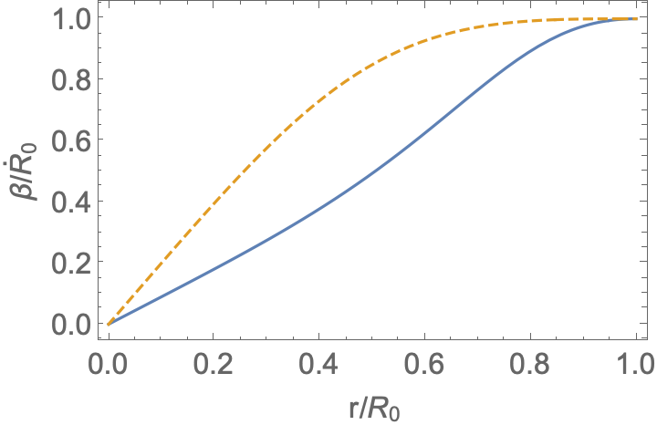
Figure 1: Velocity $|\beta_{EM}|$ of oscillating Dungey’s magnetospheres: top curve for $\theta=\pi/2$, bottom for $\theta=\pi/4$. This illustrates that the velocity of oscalailateiton is $\beta\approx r$.

The above solutions establish the large scale electromagnetic field within the magnetosphere. Next we consider particle dynamics in the given electromagnetic fields, first theoretically in §4, and then numerically in §5

4 Theory of radial diffusion in corotating magnetospheres

4.1 The three adiabatic invariants

For particles trapped on closed field lines, there are three adiabatic invariants: first associated with cyclotron motion around a field line, second associate with bouncing motion between the magnetic poles, and a third one associated with azimuthal B-cross-grad-B drift.

In the Double Pulsar, the conservations of the first invariant is assured by very short cyclotron time even at the magnetospheric boundary. The second adiabatic invariant is mildly conserved in the corotating magnetosphere, which extends nearly to the light cylinder. The bounce period for relativistic particle (second adiabatic invariant, Walt, 2005, Eq. 4.28)

$$\tau_{b}\sim 5.4{r\over c}\leq{2\pi}/\Omega_{B}$$ (4)

This is somewhat shorter than the Pulsar B period at the outer parts of the magnetosphere, and even shorter deeper inside magnetosphere – the second invariant is mostly conserved, and is well conserved in the inner regions.

Thus, similarly to the case of planetary magnetospheres, radial diffusion in the Pulsar B magnetosphere occurs through breakdown of the third adiabatic invariant: spin-induced variation of the magnetosphere lead to changing $L$ parameter. We consider this process next.

4.2 Magnetic pumping/betatron induced diffusion

As an illustration how varying magnetic field leads to diffusion, let’s consider straight magnetic field changing in time $B_{z}=B$. (This is a local approximation, hence we are not concerned with the global structure of the fields.) Choosing vector potential in the Landau gauge

$${\bf A}=-\{By,0,0\}$$ (5)

We find the Hamiltonian

$$H=\frac{(p_{x}+By)^{2}+p_{y}^{2}}{2}$$ (6)

The $x$ momentum is a conserved quantity,

$$p_{x}=p_{x,0}$$ (7)

while equation for $y$-momentum becomes

$$\partial_{t}p_{y}=-B(p_{x,0}+By)\mbox{}$$

$$\partial_{t}y=p_{y}$$ (8)

with the appropriate constants ($c,m_{e},e$) set to unity.

For harmonic variation of the field (this is to be used in the expression for vector potential (5))

$$B=B_{0}+(\delta B)\cos(\Omega t)$$ (9)

we find

$$\ddot{p}_{y}={(\delta B)}\Omega\sin(\Omega t)\left(-\frac{2\dot{p}_{y}}{{B_{0}}+{(\delta B)}\cos(\Omega t)}-{p_{x,0}}\right)-p_{y}({B_{0}}+{(\delta B)}\cos(\Omega t))^{2}\approx\mbox{}$$

$${(\delta B)}\left(-\frac{\Omega\sin(\Omega t)\left({B_{0}}{p_{x,0}}+2\dot{p}_{y}\right)}{{B_{0}}}-2{B_{0}}p_{y}\cos(\Omega t)\right)-{B_{0}}^{2}p_{y}$$ (10)

For small frequencies $\Omega\to 0$ this reduces to Mathieu’s equation

$$\ddot{p_{y}}+{B_{0}}^{2}p_{y}+2{B_{0}}{(\delta B)}\cos(\Omega t)p_{y}=0$$ (11)

Mathieu’s equation has instability bands (McLAchlan, 1947): this is the origin of radial diffusion in corotating magnetospheres.

4.3 The diffusion coefficient

The particle motion within the magnetosphere of Pulsar B obeys Mathieu’s equation. As parameters of the orbit change, particle motion occasionally becomes unstable, with large changes in the L-parameter. The motion is stochastic, but non-diffusive, periods of constant L-parameter are intermittent with periods of rapid radial evolution. To understand time-average behavior we may still use a concept of diffusion (time-averaging here means that motion is averaged over sufficiently long times, including many episodes of rapid L-evolution).

The particles trapped in the magnetosphere  of Pulsar B form the analogues of planetary radiation belts (van Allen belts). Both in planetary magnetospheres and the Pulsar B particles are injected at the magnetosheath, and then diffuse inward. The radial diffusion is achieved by breaking of the 3d adiabatic invariant (Fälthammar, 1968) and is described by radial diffusion equation

$$\partial_{t}f=\partial_{L}\left(D_{LL}{1\over L^{2}}\partial_{L}(L^{2}f)\right)$$ (12)

where $D_{LL}$ is the diffusion coefficient

The diffusion coefficient $D_{LL}$ is a product of typical velocity times typical jump in $L$. The diffusion is driven by the E-cross-B velocity oscillations, approximately $\propto L$, Fig. 1. The induced diffusions is a non-adiabatic effect, proportional to the Larmor radius of the particles. Conservation of the first adiabatic invariant implies betatron condition $\epsilon_{\perp}\propto B$ - as a result, the Larmor radius remains nearly constant as a particle diffuse inward. Thus, $D_{LL}=\kappa_{0}L$, where $\kappa$ is some constant. Then the rate of change of average value of $<L>$ is

$$\partial_{t}<L>\propto\kappa_{0}={\rm constant}$$ (13)

while the steady state is

$$f\propto\frac{1}{L}$$ (14)

Qualitatively, this is our main result: diffusion in fast corotating magnetospheres produces density of trapped particles $\propto 1/r$.

5 Simulations

5.1 Code verification

We have developed a Boris-based pusher (Boris & Roberts, 1969; Birdsall & Langdon, 1991). Particles are injected at a given radius and move in the fields given by (1), At each point the $L$ parameters is calculated according to (2). We verified that for non-rotating case $\Omega=0$ and sufficiently small Larmor radius parameter $L$ remains constant, Fig. 2.

We also verified that if initial velocity of particles is zero, they just move with the electromagnetic drift velocity (1). Non-zero initial momentum, even if directed along the local magnetic field, leads to complicated particle dynamics with changing $L$ parameter. This is due to both effects of finite Larmor radius, and various drifts.

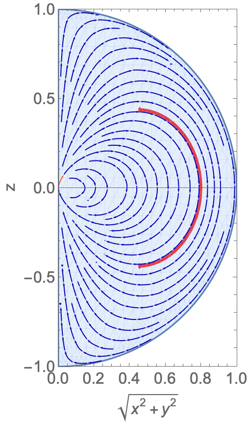
Figure 2: Example of particle motion calculated with our code in steady-state Dungey field ($z-\sqrt{x^{2}+y^{2}}$ and $x-y$ projections). Particle is injected at $L=0.8$ at the equator. It experiences bouncing motion. The parameter $L$ remains constant

5.2 Analysis of simulations

For small gyration momenta particles initially just follow the magnetic field, with extra the drift motion. But eventually gets out of phase and the trajectory becomes random. We observe that the dynamics is not of a simple diffusion type: long intervals of just periodic oscillations are interrupted by intervals of fast diffusion, Fig. 4. We attribute these changes to the complicated structure of unstable bands of the Mathieu’s equation, see (11).

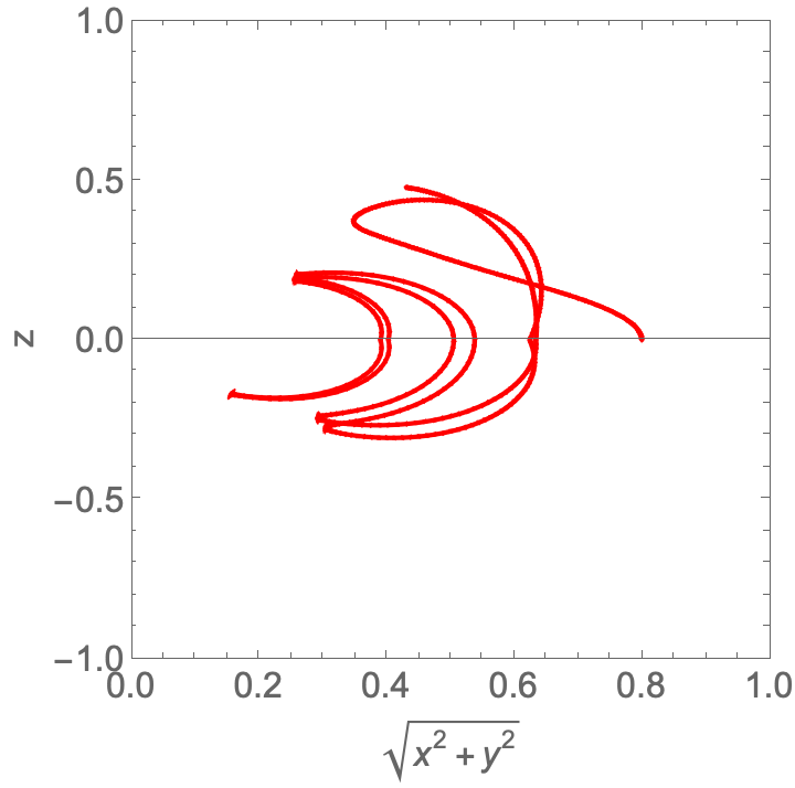
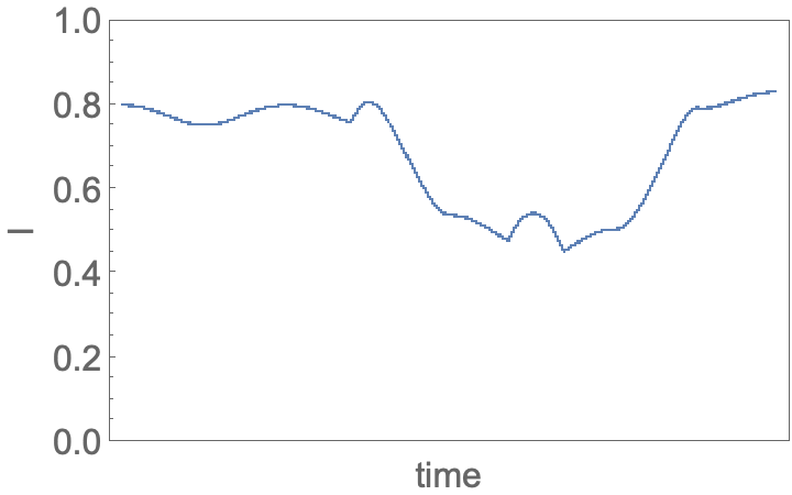
Figure 3: Particle trajectory for time-dependent oscillations of the overall radius, $\delta R=0.1$. Particle experiences diffusion in $L$ and stochastic trajectory (right panel).

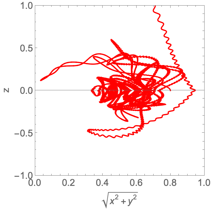
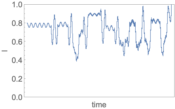
Figure 4: An example demonstrating that intervals of just periodic oscillations are often intermittent with intervals of fast diffusion. This is expected, since the particle motion is controlled by the Mathieu’s equation (11) which has stable/unstable bands depending on the parameters.

We also observe that some injected particles often quickly escape. We attribute this to the fact that the value of the E-cross-B drift is larger at larger radii. Thus, a particle oscillating along a given field line will have larger radial velocity when it is further out.

One of the main points of the present work is illustrated in Fig. 5, which shows that particles drift inwards from the injection point.

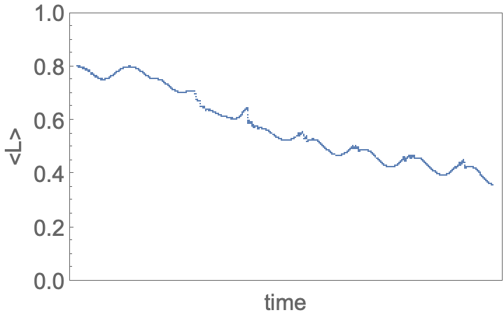
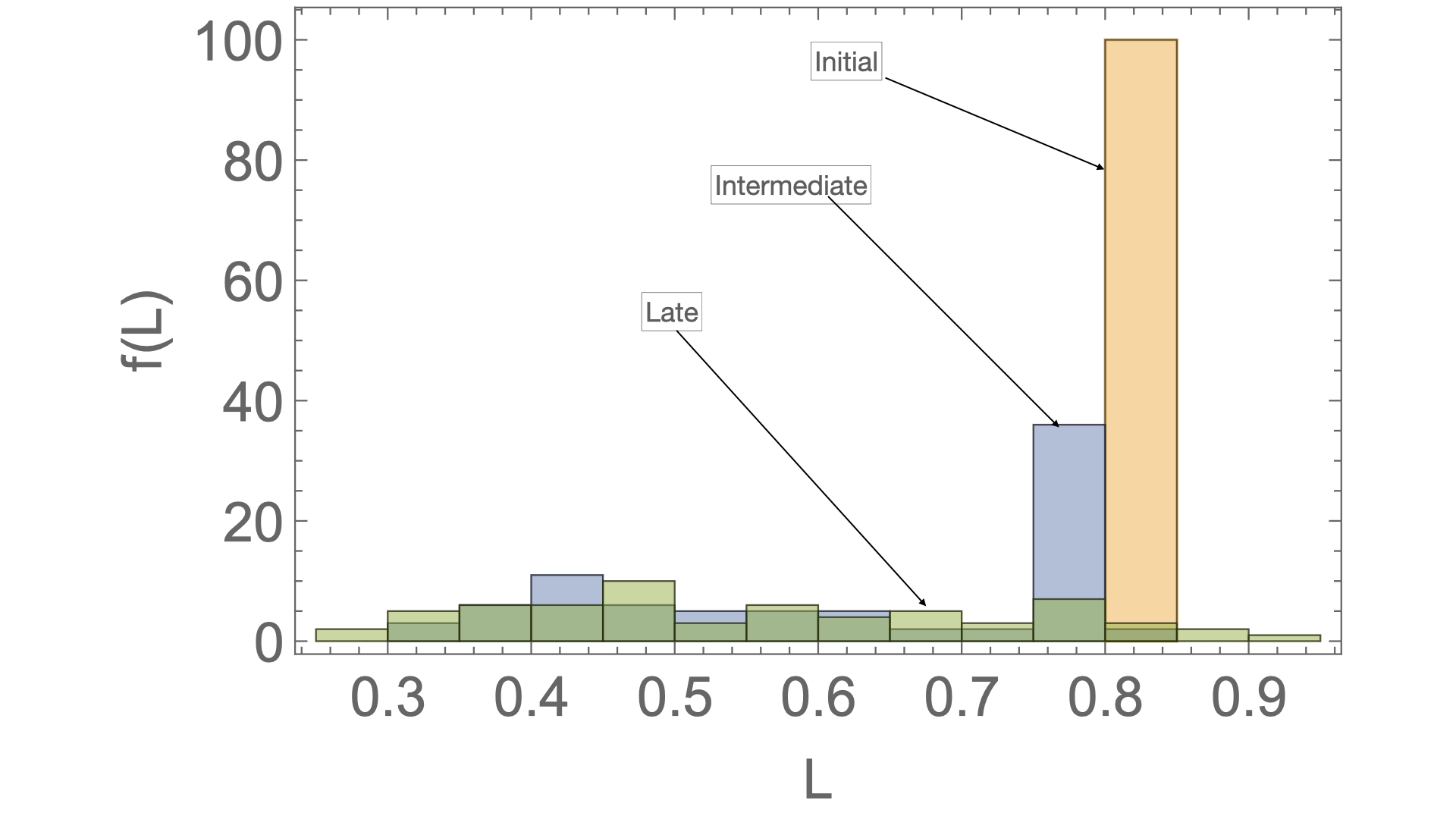
Figure 5: Left Panel: Average value of the $L$ parameter as a function of time, showing that particles on average drift inwards. Particles are injected at $L=0.8$ with the same total momentum but random direction. Right Panel: evolution of the distribution $f(L)$ - particles are injected at $L=0.8$, and generally diffuse inward.

The diffusion is not homogeneous (in a sense that it does not obey the conventional diffusion equation), but stochastic: many particles remain at a fixed $L$, until they get into the regime of a parametric resonance.

6 Radial diffusion in rotating distorted magnetosphere

Next we complement our analysis with a model of distorted and rotating confined magnetospheres, following Stern (1994); Tsyganenko (1995), (previously applied to the Double Pulsar by Lyutikov (2005)). It is a different way of modeling the distorted magnetosphere: instead of time-dependent underlying fields we construct a spatially-dependent models of rotating confined magnetic configurations. (We also note a relevant paper by Elkington et al., 2003, where a somewhat different model of the distorted planetary field was used. Importantly, the magnetosphere was not co-rotating in that study.)

First we employ the method of distortion transformation of Euler potentials (Stern, 1994; Voigt, 1981) to find magnetic field. A major advantage of the stretching model of magnetosphere is that it reproduces fairly well the structure of a tilted dipole (Stern, 1994). Next we find rotationally induced electric field, and then repeat out calculations of the trajectories. This method is somewhat different from the oscillating Dungey’s magnetosphere: in the case all the fields are stationary.

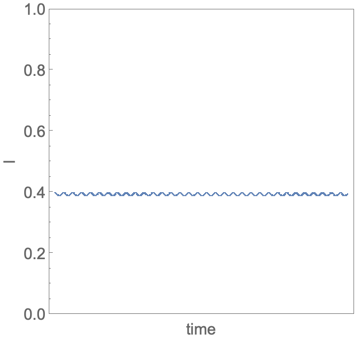
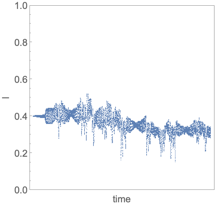
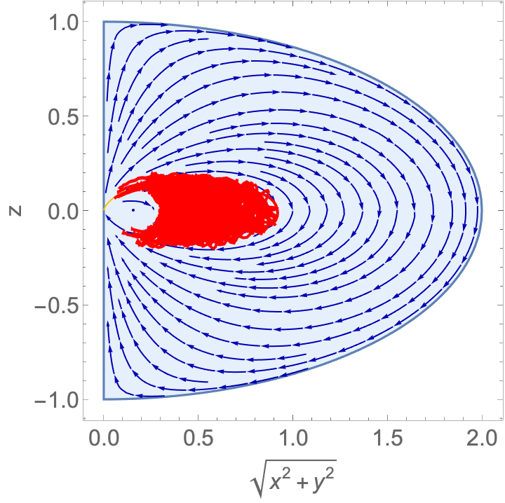
Figure 6: Top row: $\Omega=0$ case. Evolution of the L-parameter $L(t)$ (left panel) and particle trajectory $z(\sqrt{x^{2}+y^{2}})$ (right panel). Bottom row: $\Omega=0.05$. Same initial velocities, distortion parameter $C=1/2$. Initial location corresponds to $L=0.4$.

Magnetic field can be described by two Euler potentials $\alpha$ and $\beta$ (sometimes called Clebsh potentials):

$${\bf B}=\nabla\alpha\times\nabla\beta$$ (15)

so that magnetic field line is defined by an intersection of surfaces with constant $\alpha$ and $\beta$. Magnetosphere of B enshrouded by magnetopause resembles a dipole field compressed on the dayside and stretched out on the nightside. The structure of the nightside magnetosphere can be approximated by stretching transformations of the Euler potentials $\alpha$ and $\beta$.

In axially-symmetric magnetosphere,

$$\alpha=\Phi,\,\mbox{Eq. (\ref{1}), with constant $R_{0}$}\mbox{}$$

$$\beta=\phi$$ (16)

Converting to Cartesian coordinates, stretching the $x$ coordinate by transformation $x\to Cx$ we find the new Euler potentials and the magnetic field  ${\bf B}_{1}$ (relations become cumbersome so we omit then here: the procedure is clear). By construction the new field ${\bf B}_{1}$ satisfies ${\rm\,div\,}{\bf B}_{1}=0$. The shape of the cavity is

$$C^{2}x^{2}+y^{2}+z^{2}=R_{0}^{2}$$ (17)

On the surface the normal component of the magnetic field vanishes.

The $L$ parameter (2) is now defined as

$$\frac{\left(x^{2}+y^{2}\right)\left(R_{0}^{3}-\left(C^{2}x^{2}+y^{2}+z^{2}\right)^{3/2}\right)}{\left(x^{2}+y^{2}+z^{2}\right)\sqrt{C^{2}x^{2}+y^{2}+z^{2}}}=\frac{1-L^{3}}{L}$$ (18)

As novel step, let’s assume that the central star is rotating. Purely for simplicity, and to demonstrate the principal effect, let’s assume that the star’s spin is along $z$ axis, so that inside the cavity the plasma moves with constant coordinate $z$. This requires

$$C^{2}x\beta_{x}+y\beta_{y}=0$$ (19)

Thus

$$\beta_{x}=-\frac{y\Omega\sqrt{x^{2}+y^{2}}}{C^{2}x\sqrt{\frac{y^{2}}{C^{4}x^{2}}+1}}\mbox{}$$

$$\beta_{y}=\frac{\Omega\sqrt{x^{2}+y^{2}}}{\sqrt{\frac{y^{2}}{C^{4}x^{2}}+1}}$$ (20)

The electric field is then

$${\bf E}_{1}=-{\bf\beta}\times{\bf B}_{1}$$ (21)

Using fields $B_{1}$ and $E_{1}$ in the Boris pusher, we find dynamics very similar to the case of oscillating Dungey magnetosphere, Fig. 6.

The results of the two approaches (oscillating Dungey magnetosphere, and the stretched out rotating magnetosphere) show qualitatively the same picture: strong radial diffusion is induced by the rotating magnetosphere. Thus, using two complementary methods: oscillating Dungey’s magnetosphere and rotating stationary magnetosphere we arrive at the same result: betatron-type induced radial diffusion.

7 Application to Pulsar B

Let us assume that injection rate is fraction of influx of the Pulsar A wind hitting the Pulsar B magnetosphere. Pulsar A’s spindown power can be related to the particle influx at Pulsar B magnetosphere:

$$L_{A}=4\pi r_{AB}^{2}n\Gamma_{w}mc^{3}$$ (22)

where $L_{A}$ is Pulsar A’s spindown power, $r_{AB}$ is the distance between two pulsars, and $\Gamma_{w}$ is the Lorentz factor of the Pulsar A’s wind ($\sigma\sim 1$ is assumed for estimates).

The magnetosphere of Pulsar B covers approximately $10^{-3}$ of $4\pi$, as seen from Pulsar A (Lyutikov & Thompson, 2005). Let’s assume that efficiency of getting into magnetosphere is $\zeta$ (it likely depends on the orbital phase, e.g.  as a fraction of polar cap “facing the wind”). The injection rate is then

$$\dot{N}={L_{A}\eta\zeta\over\Gamma_{w}mc^{2}}$$ (23)

The density of particles in the magnetosphere is determined by the balance of the injection rate (23) and the rate at which particles fall onto the star due to radiative losses. Radiative decay rate is $N/(\kappa P_{B})$

$$\dot{N}=N/(\kappa P_{B})\mbox{}$$

$$N=\dot{N}\kappa P_{B}$$ (24)

where

$$\kappa=\frac{1}{8}\left(\frac{R_{m}}{R_{cool}}\right)^{-3}\sim 2\times 10^{-5}$$ (25)

is the inverse of a typical time (in periods of Pulsar B) that particles spend in the magnetospheres, $R_{m}=4\times 10^{9}$ cm is the radius of the wind-confined magnetosphere of Pulsar B, $R_{cool}=2.4\times 10^{8}$ cm is the cooling radius (where cooling time becomes of the order of the Pulsar B period), Lyutikov & Thompson (2005).

The equilibrium density is then

$$n={N\over(4\pi/3)R_{m}^{3}}={\dot{N}\kappa P_{B}\over(4\pi/3)R_{m}^{3}}\mbox{}$$

$$\lambda={n\over n_{GJ}}={3\pi eL_{A}\eta\kappa\zeta\over B_{m}cmR_{m}^{3}\Gamma_{w}\Omega_{B}^{2}}={3\times 10^{8}\over\Gamma_{w}/(10^{5})}$$ (26)

($\lambda$ is the over-density with respect to the Goldreich & Julian (1969)) density $n_{GJ}$). The estimate (26) exceeds the minimal density required imposed by the eclipse model of Lyutikov & Thompson (2005).

8 Discussion

In this paper we discuss an unusual regime of radial diffusion in the wind-confined magnetospheres: when the secondary (Pulsar B in this case) is fast rotating, so that the rotational period is shorter than the time scale of azimuthal drifts. In this regime the third adiabatic invariant is strongly violated just by the electromagnetic fields arising from rotational compression of the magnetosphere. No extra turbulence is needed. We demonstrate that in this case the radial diffusions is driven purely by the rotating of the central star - there is no need for turbulent pitch angle scattering to induce the radial diffusion. The radial diffusion occurs to what can be called “a betatron-induced diffusion”: fluctuations of the electric field (either in Lagrangian or Eulerian sense - the two models we considered) induce (occasional) parametric instability in particle’s orbits.

Thus, the magnetospheric boundary is indeed where Lyutikov & Thompson (2005) calculated it to be. But the density of the trapped practices increases inward - hence smaller eclipsing region, by a factor of $\sim 3$.

9 ACKNOWLEDGEMENTS

I would like to thank Mary Hudson for comments on the manuscript and Maura McLaughlin for discussions. This work had been supported by NASA grants 80NSSC17K0757 and 80NSSC20K0910, NSF grants 1903332 and 1908590.

10 DATA AVAILABILITY

The data underlying this article will be shared on reasonable request to the corresponding author.

References

- Akasofu (1964) Akasofu, S. I. 1964, Planet. Space Sci., 12, 273
- Axford & Hines (1961) Axford, W. I. & Hines, C. O. 1961, Canadian Journal of Physics, 39, 1433
- Birdsall & Langdon (1991) Birdsall, C. K. & Langdon, A. B. 1991, Plasma Physics via Computer Simulation
- Boris & Roberts (1969) Boris, J. P. & Roberts, K. V. 1969, Journal of Computational Physics, 4, 552
- Breton et al. (2008) Breton, R. P., Kaspi, V. M., Kramer, M., McLaughlin, M. A., Lyutikov, M., Ransom, S. M., Stairs, I. H., Ferdman, R. D., Camilo, F., & Possenti, A. 2008, Science, 321, 104
- Brice & Ioannidis (1970) Brice, N. M. & Ioannidis, G. A. 1970, Icarus, 13, 173
- Burgay et al. (2003) Burgay, M., D’Amico, N., Possenti, A., Manchester, R. N., Lyne, A. G., Joshi, B. C., McLaughlin, M. A., Kramer, M., Sarkissian, J. M., Camilo, F., Kalogera, V., Kim, C., & Lorimer, D. R. 2003, Nature, 426, 531
- Coroniti (1974) Coroniti, F. V. 1974, ApJS, 27, 261
- Dungey (1961) Dungey, J. W. 1961, Physical Review Letters, 6, 47
- Elkington et al. (2003) Elkington, S. R., Hudson, M. K., & Chan, A. A. 2003, Journal of Geophysical Research (Space Physics), 108, 1116
- Fälthammar (1968) Fälthammar, C.-G. 1968, in Earth’s Particles and Fields, ed. B. M. McCormac, 157
- Goldreich & Julian (1969) Goldreich, P. & Julian, W. H. 1969, ApJ, 157, 869
- Heikkila & Winningham (1971) Heikkila, W. J. & Winningham, J. D. 1971, J. Geophys. Res., 76, 883
- Iacolina et al. (2016) Iacolina, M. N., Pellizzoni, A., Egron, E., Possenti, A., Breton, R., Lyutikov, M., Kramer, M., Burgay, M., Motta, S. E., De Luca, A., & Tiengo, A. 2016, ApJ, 824, 87
- Joy et al. (2002) Joy, S. P., Kivelson, M. G., Walker, R. J., Khurana, K. K., Russell, C. T., & Ogino, T. 2002, Journal of Geophysical Research (Space Physics), 107, 1309
- Kallenrode (2004) Kallenrode, M.-B. 2004, Space physics : an introduction to plasmas and particles in the heliosphere and magnetospheres
- Kaspi et al. (2004) Kaspi, V. M., Ransom, S. M., Backer, D. C., Ramachandran, R., Demorest, P., Arons, J., & Spitkovsky, A. 2004, ApJ, 613, L137
- Kennel (1973) Kennel, C. F. 1973, Space Sci. Rev., 14, 511
- Kennel & Coroniti (1975) Kennel, C. F. & Coroniti, F. V. 1975, Space Sci. Rev., 17, 857
- Kramer & Stairs (2008) Kramer, M. & Stairs, I. H. 2008, ARA&A, 46, 541
- Kramer et al. (2006) Kramer, M., Stairs, I. H., Manchester, R. N., McLaughlin, M. A., Lyne, A. G., Ferdman, R. D., Burgay, M., Lorimer, D. R., Possenti, A., D’Amico, N., Sarkissian, J. M., Hobbs, G. B., Reynolds, J. E., Freire, P. C. C., & Camilo, F. 2006, Science, 314, 97
- Kramer & Wex (2009) Kramer, M. & Wex, N. 2009, Classical and Quantum Gravity, 26, 073001
- Li & Hudson (2019) Li, W. & Hudson, M. K. 2019, Journal of Geophysical Research (Space Physics), 124, 8319
- Lomiashvili & Lyutikov (2014) Lomiashvili, D. & Lyutikov, M. 2014, MNRAS, 441, 690
- Lyne et al. (2004) Lyne, A. G., Burgay, M., Kramer, M., Possenti, A., Manchester, R. N., Camilo, F., McLaughlin, M. A., Lorimer, D. R., D’Amico, N., Joshi, B. C., Reynolds, J., & Freire, P. C. C. 2004, Science, 303, 1153
- Lyutikov (2005) Lyutikov, M. 2005, MNRAS, 362, 1078
- Lyutikov & Thompson (2005) Lyutikov, M. & Thompson, C. 2005, ApJ, 634, 1223
- McLAchlan (1947) McLAchlan, N. 1947, Theory and Application of Mathieu Functions (Oxford University Press)
- McLaughlin et al. (2004) McLaughlin, M. A., Camilo, F., Burgay, M., D’Amico, N., Joshi, B. C., Kramer, M., Lorimer, D. R., Lyne, A. G., Manchester, R. N., & Possenti, A. 2004, ApJ, 605, L41
- Ogino et al. (1998) Ogino, T., Walker, R. J., & Kivelson, M. G. 1998, J. Geophys. Res., 103, 225
- Podsiadlowski et al. (2005) Podsiadlowski, P., Dewi, J. D. M., Lesaffre, P., Miller, J. C., Newton, W. G., & Stone, J. R. 2005, MNRAS, 361, 1243
- Ransom et al. (2004) Ransom, S. M., Kaspi, V. M., Ramachandran, R., Demorest, P., Backer, D. C., Pfahl, E. D., Ghigo, F. D., & Kaplan, D. L. 2004, ApJ, 609, L71
- Schulz & Lanzerotti (1974) Schulz, M. & Lanzerotti, L. J. 1974, Particle diffusion in the radiation belts (Physics and Chemistry in Space, Berlin: Springer, 1974)
- Sonnerup et al. (1981) Sonnerup, B. U. O., Paschmann, G., Papamastorakis, I., Sckopke, N., Haerendel, G., Bame, S. J., Asbridge, J. R., Gosling, J. T., & Russell, C. T. 1981, J. Geophys. Res., 86, 10049
- Spitkovsky & Arons (2004) Spitkovsky, A. & Arons, J. 2004, in 35th COSPAR Scientific Assembly, Vol. 35, 4117
- Stern (1994) Stern, D. P. 1994, J. Geophys. Res., 99, 17169
- Summers et al. (1998) Summers, D., Thorne, R. M., & Xiao, F. 1998, J. Geophys. Res., 103, 20487
- Thorne (2010) Thorne, R. M. 2010, Geophys. Res. Lett., 37, L22107
- Tsyganenko (1995) Tsyganenko, N. A. 1995, J. Geophys. Res., 100, 5599
- Tsyganenko (2002) —. 2002, Journal of Geophysical Research (Space Physics), 107, 1179
- Ukhorskiy et al. (2005) Ukhorskiy, A. Y., Takahashi, K., Anderson, B. J., & Korth, H. 2005, Journal of Geophysical Research (Space Physics), 110, A10202
- Voigt (1981) Voigt, G. H. 1981, Planet. Space Sci., 29, 1
- Walt (2005) Walt, M. 2005, Introduction to Geomagnetically Trapped Radiation
- Zhang et al. (2021) Zhang, B., Delamere, P. A., Yao, Z., Bonfond, B., Lin, D., Sorathia, K. A., Brambles, O. J., Lotko, W., Garretson, J. S., Merkin, V. G., Grodent, D., Dunn, W. R., & Lyon, J. G. 2021, Science Advances, 7, eabd1204