A statistical reconstruction algorithm for positronium lifetime imaging using time-of-flight positron emission tomography

Abstract

Positron emission tomography (PET) has been widely used for the diagnosis of serious diseases including cancer and Alzheimer’s disease, based on the uptake of radiolabeled molecules that target certain pathological signatures. Recently, a novel imaging mode known as positronium lifetime imaging (PLI) has been shown possible with time-of-flight (TOF) PET as well. PLI is also of practical interest because it can provide complementary disease information reflecting conditions of the tissue microenvironment via mechanisms that are independent of tracer uptake. However, for the present practical systems that have a finite TOF resolution, the PLI reconstruction problem has yet to be fully formulated for the development of accurate reconstruction algorithms. This paper addresses this challenge by developing a statistical model for the PLI data and deriving a maximum-likelihood algorithm for reconstructing lifetime images alongside the uptake images. By using computer simulation data, we show that the proposed algorithm can produce quantitatively accurate lifetime images.

I Introduction

The physics that enables positronium lifetime imaging (PLI) with time-of-flight (TOF) positron emission tomography (PET) has recently been elucidated, and the feasibility of PLI has been experimentally demonstrated [1, 2, 3, 4, 5]. PET is widely used for revealing the functional state of an organ or tissue by the uptake of a specific PET molecule as governed by its physiological and biochemical interactions with the body. On the other hand, PLI measures the lifetime of positronium, which is a meta-stable electron-positron pair formed by a positron released by a PET molecule [6]. Interactions between positronium and nearby molecules such as oxygen that contain an unpaired electron will shorten its lifetime. Therefore, the positronium lifetime can quantitatively reflect the presence and concentration of such molecules in the tissue microenvironment independent of the uptake mechanism of the PET molecule. This is of clinical interest because, for example, hypoxic tissues are resistant to many therapeutics [4, 7]. Knowing the local tissue oxygenation may lead to better treatment outcomes for cancer. Additionally, PLI could open the door for the creation of novel contrast mechanisms for PET.

Presently, PLI is demonstrated by using experimental setups that allow unambiguous separation of the events according their origins in space [8, 9]. However, the present TOF-PET systems have a coincidence resolving time (CRT) in the range of 200 - 600 ps full width at half maximum (FWHM) [10, 11, 12], corresponding to a spatial uncertainty of 3-9 cm. PLI reconstruction under finite TOF resolutions is a topic of interest and significance.

This issue potentially can be addressed by the development of a statistical model relating the unknown uptake and lifetime images to the PLI data to allow inversion of the data. to avoid information loss due to averaging. The inverse Laplace transform method has been proposed for separating the lifetime components in a voxel [13]. So far, this idea has only been investigated by Qi and Huang [14]. We call such approach as the penalized surrogate (PS) method in this article. In their models, the lifetime measurement does not include the effects of the finite time resolution of the detectors or the difference in the flight time of the gamma rays associated with an event before they are detected. The main contribution of this paper is the development of a more complete model for the 2-dimensional PLI data. We also develop a computationally efficient algorithm using the Limited-memory Broyden-Fletcher-Goldfarb-Shanno Bound (L-BFGS-B) method available from scipy.optimize [15], including the positivity condition for producing the maximum likelihood (ML) estimator of this model. Using computer-simulated data, we demonstrate that the resulting algorithm can accurately recover the lifetime image from data acquired by TOF-PET systems.

The remainder of this paper is organized as follows. Section II formulates the statistical model for the PLI list-mode data and uses the model to develop an algorithm for obtaining the maximum likelihood estimates of both uptake and lifetime images. Section III describes the computer-simulation study and presents the results. Section IV provides a summary and conclusion.

II Statistical model for PLI

II-A Detection of a PLI event

Figure 1 illustrates the use of a two-dimensional (2d) TOF-PET system that consists of a ring of uniformly spaced detectors. Contrary to the traditional PET, PLI uses an isotope such as Sc-44 that emits a positron and a prompt gamma essentially at the same time [16, 17]. Such isotope has a much larger positron range than a typical F-18 used in PET, which can drastically deteriorate spatial resolution [18]. In this work, as in [14] positron range is ignored.

Suppose that an isotope decay occurs at location ${\bm{r}}_{decay}$ at time $t_{decay}$. As depicted by the blue line in the figure, the prompt gamma travels a distance $\alpha_{\gamma}$ from ${\bm{r}}_{decay}$ towards the detector ring at a random angle $\phi_{\gamma}$, detected by detector $i_{\gamma}$ at time $t_{\gamma}=t_{decay}+\alpha_{\gamma}/v_{c}$, where $v_{c}$ is the speed of light.

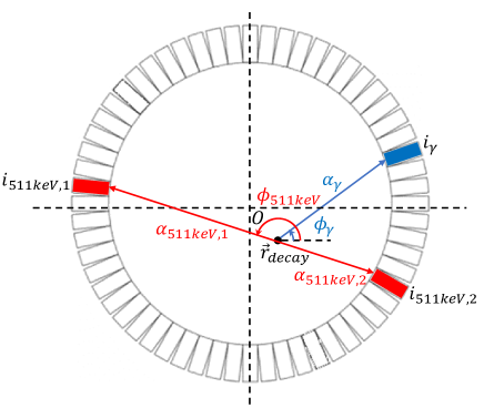
Figure 1: Detection of a PLI event using 2-d TOF-PET system.

There are three lifetime components, only the ortho-positronium (o-Ps) component is sensitive to the environment and therefore is of interest, and the single exponential approximation is accurate except for small tau because the o-Ps lifetime is the longest. In this article we focus on the o-Ps mean lifetime that is affected by the properties of neighboring tissues. We will consider the multiexponential distribution for our future research work. The exponential distribution in Eq. (1) that is reasonable for the o-Ps lifetime distribution [8] is described as follows. The released positron annihilates after time $\tau$ that follows an exponential distribution $\mbox{Exp}(\tau;\lambda)$ defined by

$$f(\tau;\lambda)=\lambda e^{-\lambda\tau},\ \tau\geq 0,$$ (1)

and $f(\tau;\lambda)=0$ for $\tau<0.$ The decay rate constant $\lambda$ (whose inverse $\lambda^{-1}$ is the lifetime) depends on the condition surrounding the positronium. The red line in the Fig. 1 illustrates the two opposite 511 keV gamma rays by annihilation. They travel from ${\bm{r}}_{decay}$ at a random angle $\phi_{511keV}$ and are detected by detectors $i_{511keV,1}$ and $i_{511keV,2}$ at time $t_{511keV,1}=t_{decay}+\tau+\alpha_{511keV,1}/v_{c}$ and $t_{511keV,2}=t_{decay}+\tau+\alpha_{511keV,2}/v_{c}$ respectively, where $\alpha_{511keV,1}$ and $\alpha_{511keV,2}$ are the photon travelling distances that these photons travel.

The conventional TOF-PET system reports $i_{511keV,1}$, $i_{511keV,2}$, and the TOF given by

$$\Delta t_{511keV}=t_{511keV,1}-t_{511keV,2}=(\alpha_{511keV,1}-\alpha_{511keV,2})/v_{c}.$$ (2)

We assume that the system is extended to be capable of triple-coincidence detection and reports additionally $i_{\gamma}$ and

$$\Delta t_{\gamma} =(t_{511keV,1}+t_{511keV,2})/2-t_{\gamma}$$

$$=\tau+(\alpha_{511keV,1}+\alpha_{511keV,2}-2\alpha_{\gamma})/(2v_{c}).$$ (3)

Note that $\alpha_{511keV,1}+\alpha_{511keV,2}$ can be determined from $i_{511keV,1}$ and $i_{511keV,2}$ because it equals the distance between the corresponding detectors. Additionally, if $\Delta t_{511keV}$ is exactly known, ${\bm{r}}_{decay}$ can be identified, and then $\alpha_{\gamma}$ can be computed from $i_{\gamma}$ and ${\bm{r}}_{decay}$. Then, Eq. (3) can be used to compute $\tau$ from $\Delta t_{\gamma}.$

In a real system, the time measurement has limited precision and is typically binned and stored as integers. CRT refers to the uncertainty of $\Delta t_{511keV}$ in FWHM. With a finite CRT, ${\bm{r}}_{decay}$ cannot be precisely determined. A CRT of 200 ps to a 600 ps corresponds to an uncertainty of 3 cm to 9 cm uncertainty in ${\bm{r}}_{decay}$. $\Delta t_{\gamma}$ also has limited precision and is binned has limited precision. Hence, in Eq. (3) $\alpha_{\gamma}$ is not precisely observed and all the time measurements involved contain statistical variations.

II-B Probability model of the PLI list-mode data

In conventional PET, the measured data is assigned to the line of response (LOR) $\mathcal{L}(i_{511keV,1},i_{511keV,2})$ that connects the two detectors $i_{511keV,1}$ and $i_{511keV,2}$ that detect the annihilation photons. In TOF-PET, an LOR is further divided into a number of non-overlapping segments and an event detected at the LOR is assigned to one of these segments according to the measured TOF value. In the literature, a specific TOF bin on a specific LOR is sometimes referred to as a line of segment (LOS). In this paper, the LOS will be indexed by a multi-index $c=(i_{511keV,1},i_{511keV,2},t)$ to identify the TOF bin $t$ on the LOR $\mathcal{L}(i_{511keV,1},i_{511keV,2})$. A PLI event is represented by $w=(c,i_{\gamma}$, $\Delta t_{\gamma})$ where $c$ identifies the LOS for the annihilation photon, $i_{\gamma}$ identifies the detector that receives the prompt gamma, and $\Delta t_{\gamma}$, as defined in Eq. (3), is the time difference between the detections of the annihilation photons and the prompt gamma. The detected PLI events are then given as a list of $w_{k}=(c_{k},i_{\gamma,k},\Delta t_{\gamma,k})$, where $k=1,\cdots,N_{k}$ is the event index and $N_{k}$ is the total number of events acquired. This PLI list-mode (LM) data is denoted by $\mathcal{W}_{N_{k}}=\{w_{k}\}_{k=1}^{N_{k}}$.

II-B1 Calculation of the system matrix

An element $H_{c,j}$ of the system matrix $\bm{H}$ is proportional to the probability that a positron decay occurring inside image pixel $j$ would give rise to an event at LOR $c$. The system matrix is pre-computed and stored as follows. Given $i_{511keV,1}$ and $i_{511keV,2}$, we applied the ray-tracing method that we previously implemented for computed tomography [19] to identify all pixels that $\mathcal{L}(i_{511keV,1},i_{511keV,2})$ intersects with, as well as the two intersections at the boundaries of these pixels. For one of these intersecting pixels, say $j^{\prime}$, a Gaussian function whose width equals the CRT is placed along the LOR, centered at the midpoint between the intersecting boundary points of the pixel. Then, the area of this function within each TOF bin is calculated by using $(2/\sqrt{\pi})\int_{a}^{b}e^{-t^{2}}dt=\textrm{erf}(b)-\textrm{erf}(a)$, where $\textrm{erf}(x)$ is the error function. The calculated areas give $H_{(i_{511keV,1},i_{511keV,2},k),j^{\prime}}$, $\forall k$. For all other pixels $j$ that does not intersect with the LOR, we set $H_{(i_{511keV,1},i_{511keV,2},k),j}=0,\forall k$.

II-B2 Maximum likelihood estimation

The PLI LM dataset includes the traditional TOF-PET LM data $\mathcal{C}_{N_{k}}=\{c_{k}\}_{k=1}^{N_{k}}$. We consider images ${\bm{f}}=[f_{j}]$ and ${\bm{\lambda}}=[\lambda_{j}]$ with $f_{j}\geq 0$ and $\lambda_{j}\geq 0$ which are the PET isotope concentration and positronium decay rate constant within voxel $j$. We derive the likelihood function of $(\bm{\lambda},\bm{f})$ in the appendix. The log-likelihood of $(\bm{\lambda},\bm{f})$ with the Gaussian blur using the convolution of a Gaussian distribution and an exponential distribution given $\mathcal{W}^{0}_{N}$ is

$$\ell(\bm{\lambda},\bm{f};\mathcal{W}^{0}_{N})=\sum_{k=1}^{N_{k}}\log\left(\sum_{j=1}^{N_{j}}H_{c_{k},j}f_{j}\mbox{EMG}(\tau_{k};\lambda_{j},\sigma^{2})\right),$$ (4)

where an exponentially modified Gaussian (EMG) distribution

$$\mbox{EMG}(\tau_{k};\lambda,\sigma^{2})=\frac{1}{2}\lambda_{j}e^{-\lambda_{j}(\tau_{k}-\frac{1}{2}\sigma^{2}\lambda_{j})}\left(1+\mbox{erf}\left(\frac{\tau_{k}-\lambda_{j}\sigma^{2}}{\sqrt{2}\sigma}\right)\right).$$

We derive the maximum likelihood estimation (MLE) based on the true $\tau_{k}$ like the model in [14], and denote the PLI LM data as $\mathcal{W}^{0}_{N_{k}}=\{w_{k}^{0}\}_{k=1}^{N_{k}}$, where $w_{k}^{0}=(c_{k},\tau_{k}).$ The MLE of $\bm{\lambda}$ based on the profile log-likelihood of $({\bm{\lambda}},\hat{\bm{f}})$ given $\mathcal{W}^{0}_{N_{k}}$ is

$$\footnotesize\arg\max_{\bm{\lambda}}\ell({\bm{\lambda}};\hat{\bm{f}},\mathcal{W}^{0}_{N_{k}})=\arg\max_{\bm{\lambda}}\sum_{k=1}^{N_{k}}\log\left(\sum_{j=1}^{N_{j}}H_{c_{k},j}\hat{f}_{j}\mbox{EMG}(\tau_{k};\lambda_{j},\sigma^{2})\right),$$ (5)

where the MLE of ${\bm{f}}$, $\hat{\bm{f}}$ based on the marginal log-likelihood of ${\bm{f}}$ given $\mathcal{C}_{N_{k}}$ is

$$\arg\max_{{\bm{f}}}\ell({\bm{f}};\mathcal{C}_{N_{k}})=\arg\max_{{\bm{f}}}\sum_{k=1}^{N_{k}}\log\left(\sum_{j=1}^{N_{j}}H_{c_{k},j}f_{j}\right).$$ (6)

Here $N_{j}$ is the number of image pixels. Please read the details about the log-likelihoods in the appendix.

We use the maximum likelihood expectation maximization (MLEM) algorithm for estimating ${\bm{f}}$ [20]. The ML estimates for ${\bm{f}}$ and ${\bm{\lambda}}$ are obtained from the above log likelihoods using gradient-based methods. The gradient of $\ell({\bm{\lambda}},{\bm{f}};\mathcal{W}^{0}_{N_{k}})$ with respect to ${\bm{\lambda}}$ is shown in the appendix.

III Computer-simulation studies

The PLI LM data $\mathcal{W}_{N_{k}}$ was generated by Monte-Carlo methods for a scanner that consists of $N_{det}$ detectors uniformly spaced on a ring of diameter $D$. Given $\bm{f}$, an image pixel $j$ is randomly sampled according to $\bm{f}$, where $f_{j}$ gives the relative probability for it to occur in pixel $j$ given a decay. Then, a point ${\bm{r}}_{decay}=(x_{decay},y_{decay})^{T}$ that falls inside the area of the pixel $j$: $A_{j}=[x_{j},x_{j}\pm\Delta x/2)\times[y_{j},y_{j}\pm\Delta y/2)$, where $(x_{j},y_{j})$ is the coordinate of the center of pixel $j$, $\Delta x$ and $\Delta y$ are the pixel sizes along the $x$ and $y$ directions, is sampled from $\mathcal{U}_{A_{j}}$, where $\mathcal{U}_{S}$ represents a uniform distribution over set $S$. A prompt gamma is emitted at ${\bm{r}}_{decay}$ at an angle $\phi_{\gamma}$ that is sampled from $\mathcal{U}_{[0,2\pi)}$. Then, $\alpha_{\gamma}$, the distance the prompt gamma travels before detection, is a solution of the following equation

$$|{\bm{r}}_{decay}+\alpha_{\gamma}\hat{\bm{\phi}}_{\gamma}|=D/2,$$ (7)

where $\hat{\bm{\phi}}=(\cos\phi,\sin\phi)^{T}$ is the unit vector in the direction of $\phi$. This equation has two solutions given by

$$\alpha_{\gamma}^{\pm}=-\hat{\bm{\phi}}_{\gamma}^{T}{\bm{r}}_{decay}\pm\sqrt{(\hat{\bm{\phi}}_{\gamma}^{T}{\bm{r}}_{decay})^{2}-||{\bm{r}}_{decay}||^{2}+D^{2}/4}.$$ (8)

These solutions correspond to the distances traveled in angle $\phi_{\gamma}$ and $\phi_{\gamma}+\pi$. Since $\phi_{\gamma}$ is sampled from $\mathcal{U}_{[0,2\pi)}$, we can arbitrarily choose one of these solutions, say $\alpha_{\gamma}^{+},$ without affecting the distribution of $\alpha_{\gamma}$. The detector $i_{\gamma}$ is determined using the location ${\bm{r}}_{detect}={\bm{r}}_{decay}+\alpha_{\gamma}^{+}\hat{\bm{\phi}}_{\gamma}$, where the prompt gamma hits the detector ring at

$$i_{\gamma}=\left\lfloor\left(\frac{N_{det}}{2\pi}\right)\measuredangle{\bm{r}}_{detect}\right\rfloor,$$ (9)

where $\measuredangle{\bm{r}}$ denotes the angle of $\bm{r}$ and $\lfloor x\rfloor$ is the largest integer that is smaller than or equal to $x$.

For the annihilation photons, we also sample an emission angle $\phi_{511keV}$ from $\mathcal{U}_{[0,2\pi)}$. Replacing $\phi_{\gamma}$ in Eq. (8) with $\phi_{511keV}$ yields two solutions $\alpha_{511keV,1}$ and $\alpha_{511keV,2}$, which are the distances traveled by the two opposite photons. We then employ Eq. (9) with obvious substitutions to obtain $i_{511keV,1}$ and $i_{511keV,2}$. Then, $\tau\sim\mbox{Exp}(\tau;\lambda_{j})$; i.e., a $\tau$ is sampled from $\mbox{Exp}(\tau;\lambda_{j})$. The detection time of the annihilation photons and prompt gamma with respect to $t_{decay}$, the time of positron decay, are calculated by $t_{511keV,1}=\tau+|\alpha_{511keV,1}|/v_{c}$, $t_{511keV,2}=\tau+|\alpha_{511keV,2}|/v_{c}$, and $t_{\gamma}=|\alpha_{\gamma}|/v_{c}$. To account for the uncertainty in time measurement, these values are replaced by $t_{511keV,1}^{\prime}\sim\mathcal{N}(t_{511keV,1},\sigma^{2})$, $t_{511keV,2}^{\prime}\sim\mathcal{N}(t_{511keV,2},\sigma^{2})$, and $t_{\gamma}^{\prime}\sim\mathcal{N}(t_{\gamma},\sigma^{2})$ where $\sigma^{2}=(\textrm{CRT}/2\sqrt{2\ln 2})^{2}/2$ and $\mathcal{N}(\mu,\sigma^{2})$ is a Gaussian distribution with mean $\mu$ and variance $\sigma^{2}$. Then, we compute $\Delta t^{\prime}_{511keV}=t^{\prime}_{511keV,2}-t^{\prime}_{511keV,1}$ and $\Delta t^{\prime}_{\gamma}=(t^{\prime}_{511keV,2}+t^{\prime}_{511keV,1})/2-t^{\prime}_{\gamma}$, and discretize them according to the width of TOF bins of the simulated system. From Eq. (3), we obtain the measured lifetime as

$$\tau^{\prime}=\Delta t^{\prime}_{\gamma}-\frac{\alpha_{511keV,1}+\alpha_{511keV,2}-2\alpha_{\gamma}}{2v_{c}}.$$ (10)

We generate PLI LM data as described above with $N_{det}=364$, $D=57.2$ cm, and $CRT=570$ ps. Thirteen 285 ps-width time bins were used. These settings yield $1.72$ million TOF-PET channels. As in [14], $\lambda_{j}^{-1}$ was also estimated by backprojecting (BP) the events into pixels according to $\bm{H}$ and then taking the average of $\tau^{\prime}_{k}$. For each pixel $j$,

$$(\hat{\bm{\lambda}}^{-1}_{BP})_{j}=\frac{\sum_{k}H_{c_{k},j}\tau^{\prime}_{k}}{\sum_{k}H_{c_{k},j}}.$$ (11)

We refer to the above backprojecting and the proposed MLE reconstruction methods as BP and ML, respectively.

We considered two numerical phantoms, shown in Fig. 2, for evaluating the proposed reconstruction method. Phantom 1’s rate-constant image contains four discs that have different $\lambda$ values: $0.4$ and $0.6$ ns^-1 from the background: $0.0$ ns^-1. The rate-constant image contains two 3.4 cm diameter discs with different $\lambda$ values: $0.4$ and $0.6$ ns^-1 from the background: $0.0$ ns^-1 in phantom 2. The expected number of events to generate were 1.5 million and 1 million, respectively, for phantom 1 and phantom 2. Here we only consider valid triple-coincidence events described by $w_{k}=(c_{k},\tau_{k})$. The effects of attenuation, scattering, and random events are beyond the scope of this manuscript, and hence not included in the simulation. All images are discretized into square pixels of 3.27$\times$3.27 mm², with 41$\times$41 pixels for phantom 1, and 65$\times$65 pixels for phantom 2.

IV Results

IV-A Activity and decay rate constant reconstruction

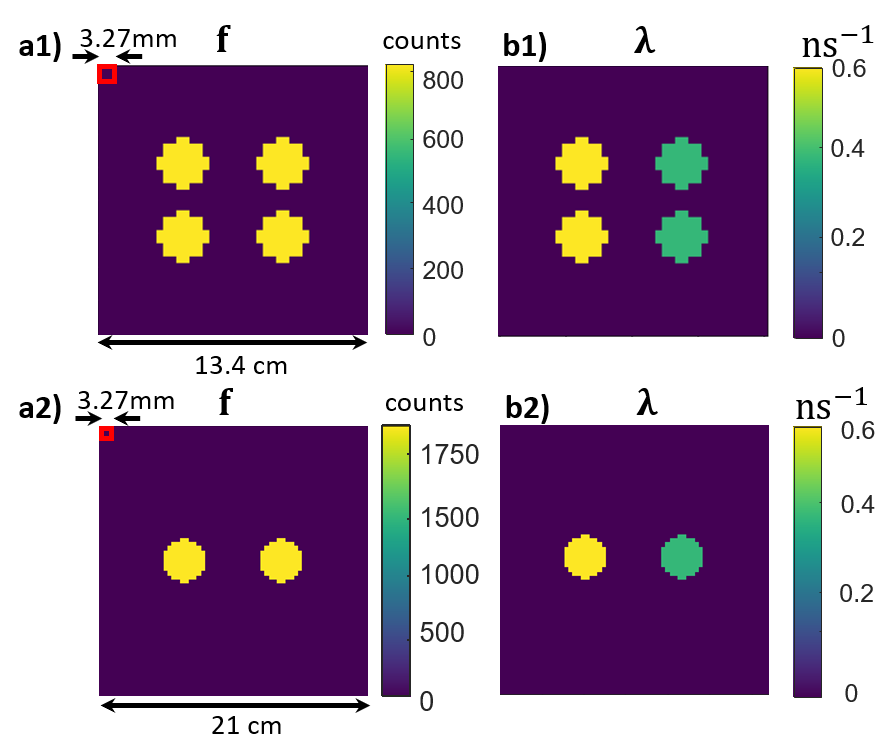
Figure 2: Activity images (left column) and rate-constant images (right column) of phantom 1 (top row) and phantom 2 (bottom row). These images consists of 3.27$\times$3.27 mm² square pixels.

Figure 3 compares images obtained for phantom 1 by the proposed ML method, the penalized surrogate method with $\beta=10$ and the number of iterations $m=5$, and the BP method. We use the following formula to estimated $\hat{\bm{\lambda}}_{BP}$ of the penalized surrogate (PS) method:

$$\hat{\lambda}_{j}^{(m+1)}=\frac{\sum_{k=1}^{N_{k}}u_{c_{k},j}^{(m)}}{\beta_{j}^{m}+\sum_{k=1}^{N_{k}}u_{c_{k},j}^{(m)}\tau^{\prime}_{k}},$$ (12)

where $\beta_{j}^{m}=\eta_{j}^{m}\beta$ is an adjusted regularized parameter for pixel j and $\eta_{j}^{m}$ is an integer between $\pm$ the number of neighborhoods of pixel $j$ (the details of the three cases of choosing $\eta_{j}^{m}$ is described in the appendix of [14]) and

$$u_{c_{k},j}^{(m+1)}=\frac{H_{c_{k},j}\hat{f}_{j}\lambda_{j}^{(m)}\mbox{EMG}(\tau^{\prime}_{k};\lambda_{j}^{(m)},\sigma^{2})}{\sum_{l=1}^{N_{j}}H_{c_{k},l}\hat{f}_{l}\lambda_{j}^{(m)}\mbox{EMG}(\tau^{\prime}_{k};\lambda_{l}^{(m)},\sigma^{2})}.$$

Notice that the method in [14] uses an exponential likelihood for the lifetime decay, but here we use the EMG likelihood in order to compare with the proposed ML method, which uses the EMG likelihood.

We also quantify the reconstruction accuracy with the normalized mean square error (NMSE), defined by

$$\text{NMSE}=\frac{\|\hat{\bm{\lambda}}-{\bm{\lambda}}\|^{2}}{\|{\bm{\lambda}}\|^{2}},$$ (13)

where $\hat{\bm{\lambda}}$ and $\bm{\lambda}$ are the reconstructed and ground-truth images, respectively, and $\|\cdot\|$ is the Euclidean norm. CRT $=570$ ps corresponds to a spatial uncertainty of 8.5 cm, which is larger than half of the largest dimension of the phantom. As a result, Fig. 3(b) shows a significantly blurred $\hat{\bm{\lambda}}_{BP}$ and the four discs can be barely seen. In contrast, Fig. 3(a1) shows that the four discs are distinct from the background in $\hat{\bm{\lambda}}_{ML}$ obtained by the proposed method. Their edges are also well identifiable. Fig. 3(c) compares the horizontal profiles across the center of the reconstructed and ground-truth images, showing that the profile of $\hat{\bm{\lambda}}_{ML}$ agrees with the truth and that of $\hat{\bm{\lambda}}_{BP}$ is almost flat. The NMSEs of $\hat{\bm{\lambda}}_{ML}$ , $\hat{\bm{\lambda}}_{PS}~{}$and $\hat{\bm{\lambda}}_{BP}$ are $0.11$, $3.32$, and $7.26$. Our proposed method provides better accuracy than the penalized method in the horizontal profile plots in Fig. 3(c) and Fig. 4(c) and overall images because the penalized method could not perform well especially the pixels on the edge of phantoms. The results further show that the BP method cannot produce a useful estimate of $\bm{\lambda}$ given the poor CRT of the simulated system, but the proposed method can produce a qualitatively and quantitatively better estimate of $\bm{\lambda}$. Figure 4 shows the results obtained for phantom 2. The NMSEs of $\hat{\bm{\lambda}}_{ML}$ , $\hat{\bm{\lambda}}_{PS}~{}$ with m = 1 and $\hat{\bm{\lambda}}_{BP}$ are $0.10$, $0.24$, and $21.65$, respectively.

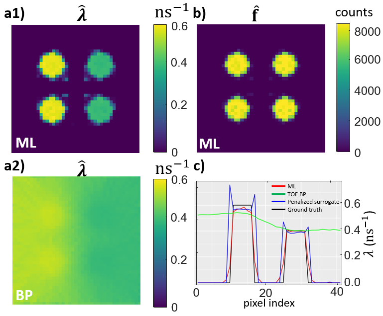
Figure 3: Results obtained for phantom 1. $\hat{\bm{\lambda}}_{ML}$ and $\hat{\bm{f}}_{ML}$ in panels a1) & b) produced by the proposed reconstruction method. (b) $\hat{\bm{\lambda}}_{BP}$ in panel a2) produced by using Eq. (11). (c) Horizontal profiles across the center of the reconstructed images $\hat{\bm{\lambda}}_{BP}$, $\hat{\bm{\lambda}}_{PS}$ and $\hat{\bm{\lambda}}_{ML}$, and of the ground-truth image $\bm{\lambda}$ in panel c).

We observe that $\bm{f}$ and $\bm{\lambda}$ of this phantom have different spatial patterns. Since estimation of $\bm{\lambda}$ depends on $\bm{f}$, potentially the resulting $\hat{\bm{\lambda}}$ can contain patterns of $\bm{f}$ if the reconstruction method is not accurate. Here we quantify the cross-talks between the activity map and the decay rate constant map with the cross-correlation, which is defined as the inner product of the residue of $\hat{\bm{\lambda}}$ and $\bm{f}$ normalized by the the Euclidean norms of $\bm{f}$ and $\hat{\bm{\lambda}}$ as follows:

$$C:=\frac{(\hat{\bm{\lambda}}-\bm{\lambda})^{T}\cdot\bm{f}}{\|\bm{\lambda}\|\|\bm{f}\|}.$$ (14)

The small cross-correlations shown in Table I using the ML, penalized surrogate, and BP methods for phantoms 1 and 2 indicate that the cross-talks from $\bm{f}$ into $\hat{\bm{\lambda}}$ are negligible.

Correlation
Phantom	Proposed	Penalized	Back
	method	surrogate	projection
1	$-3.37\times 10^{-2}$	$-4.12\times 10^{-2}$	$-5.56\times 10^{-2}$
2	$-2.11\times 10^{-2}$	$-4.99\times 10^{-2}$	$-7.39\times 10^{-2}$

TABLE I: Comparisons of the cross-correlations using the three methods for two phantoms.

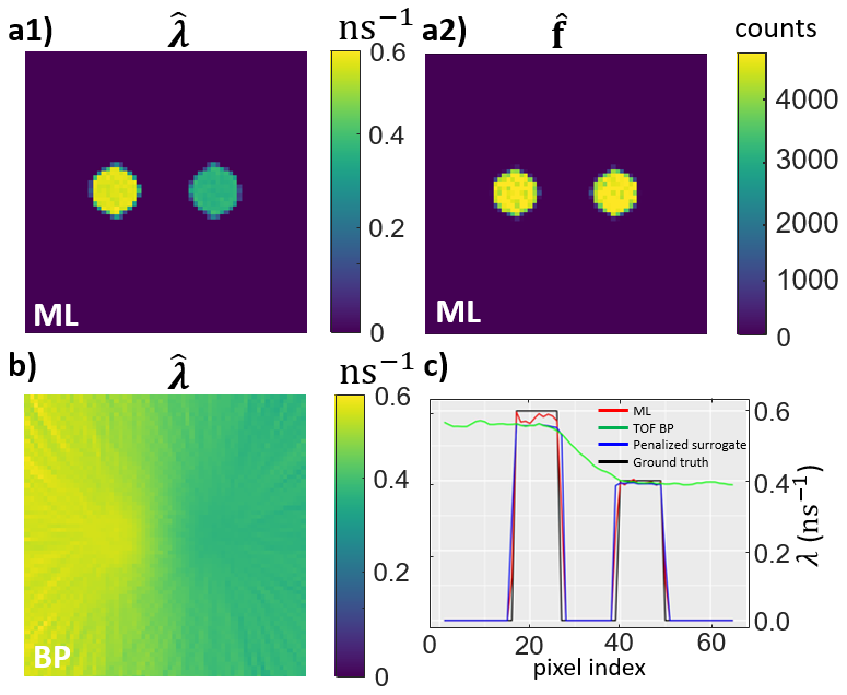
Figure 4: Results obtained for phantom 2. $\hat{\bm{\lambda}}_{ML}$ and $\hat{\bm{f}}_{ML}$ in panels a1) & a2) produced by the proposed reconstruction method. (b) $\hat{\bm{\lambda}}_{BP}$ in panel b) produced by using Eq. (11). (c) Horizontal profiles across the center of the two two discs the reconstructed images $\hat{\bm{\lambda}}_{ML}$ and $\hat{\bm{\lambda}}_{ML}$, and of the ground-truth image $\bm{\lambda}$ in panel c).

IV-B Effects of CRT

To understand the effect of different CRTs on our ML-based reconstruction method, we performed reconstructions from simulated events with CRT values 200, 400 and 600 ps using a phantom with activity and lifetime decay rate maps shown in Fig. 7.

The width of time bin was selected to be equal to $CRT/2$. The number of events is 3 million for generating all the list mode events. At each of the CRT value, ten independent Monte Carlo instances were generated for testing the reconstruction performance. Fig. 7 shows the average of the NMSE of the reconstructed decay rate constant map using an Exponential distribution for the lifetime decays (Exp-MLE), and the proposed MLE using an Exponential modified Gaussian distribution for the lifetime decays (EMG-MLE). A larger CRT contributes to higher uncertainty in the estimated lifetime $\tau^{\prime}_{k}$ associated with each event, leading to higher NMSE. The results of the MLE using our proposed methods and Exponential distribution indicate that a smaller CRT always contributes to better reconstruction and EMG-MLE consistently yields lower NMSE compared to Exp-MLE for different CRTs. Furthermore, Fig. 8 compares the horizontal profiles across the center of the two top discs of the ground truth $\bm{\lambda}$ map and the reconstructed images obtained by the EMG-MLE and Exp-MLE. These results demonstrate that EMG-MLE consistently achieves superior accuracy for all CRT values.

IV-C Comparisons of different approaches

Bias² and variance of $\hat{\bm{\lambda}}_{ML}$, $\hat{\bm{\lambda}}_{PS}$ and $\hat{\bm{\lambda}}_{BP}$ are used to evaluate the performances of these three methods given $\bm{f}$ and $\hat{\bm{f}}$ on phantom 1. Five simulations were generated independently. The results shown in Table II. indicate that the bias² and variance of $\hat{\bm{\lambda}}$ reconstructed by our method perform better than those of reconstructed by the penalized surrogate method. The bias² and variance produced by our method and the penalized surrogate method using the true $\bm{f}$ are less than those using $\hat{\bm{f}}$. This means that true $\bm{f}$ provides more accuracy than the estimated $\bm{f}$. While the bias² of $\bm{f}$ constructed by the penalized surrogate method is slightly less than the bias² using our proposed method, our proposed method results in much more smaller bias² and variance using $\hat{\bm{f}}$. The $\hat{\bm{\lambda}}_{ML}$ has less variation than the penalized surrogate method in both $\bm{f}$ and $\hat{\bm{f}}$.

Given	Quantitative	Proposed	Penalized	Back
	comparison	method	surrogate	projection
$f$	Bias2	$3.67\times 10^{-3}$	$2.14\times 10^{-3}$	$7.25$
	Variance	$9.89\times 10^{-6}$	$1.40\times 10^{-5}$	$6.07\times 10^{-5}$
$\hat{\bm{f}}$	Bias2	$1.11\times 10^{-1}$	$2.17$	$7.25$
	Variance	$2.69\times 10^{-4}$	$6.73\times 10^{-1}$	$6.07\times 10^{-5}$

TABLE II: Comparisons of bias² and variance.

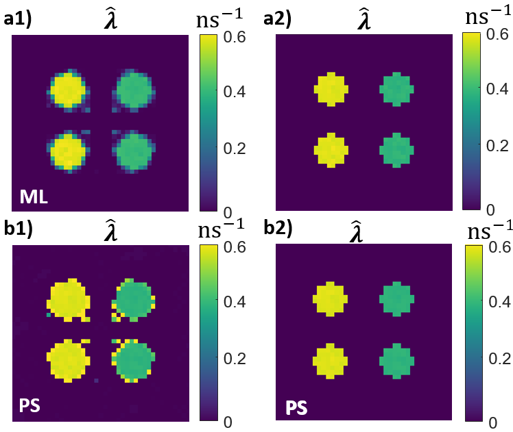
Figure 5: Results obtained for phantom 1. (a1 & a2) $\hat{\bm{\lambda}}_{ML}$ and $\hat{\bm{\lambda}}_{ML}$ produced by the proposed reconstruction method with $\hat{\bm{f}~{}}$ and $~{}\bm{f}$ respectively. (b1 & b2) $\hat{\bm{\lambda}}_{PS}$ produced by the penalized surrogate method [14] with $\hat{\bm{f}~{}}$ and $~{}\bm{f}$, respectively.

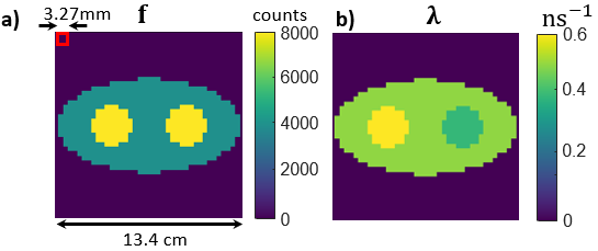
Figure 6: The activity map (a) and the lifetime decay rate map (b) of a 13.4 cm phantom with pixel size of 3.27 mm used for the ML reconstructions under different CRTs in Fig. 7.

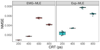
Figure 7: The NMSEs of the 10 replications of $\bm{\lambda}$ reconstruction as a function of CRT. The insets show the reconstructed decay rate constant maps using the number of events $3$ million

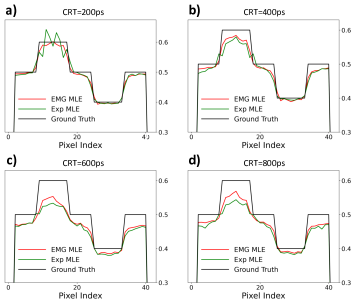
Figure 8: The cross-section at the center of the two top discs of the reconstructed $\hat{\bm{\lambda}}_{ML}$ and the true $\bm{\lambda}$ (red: EMG-MLE, green: Exp-MLE) for Phantom 1, where the reconstructed $\hat{\bm{\lambda}}_{ML}$ is averaged from 10 simulations. (a) CRT = 200 ps. (b) CRT = 400 ps. (c) CRT = 600 ps. (d) CRT = 800 ps.

We compare the the estimated $\lambda$ maps using the proposed EMG-MLE and the penalized surrogate (PS) methods in Fig. 5. We further access the reconstruction accuracy of the MLE using an Exponential distribution for the lifetime decays (Exp-MLE), and the proposed MLE using an Exponential modified Gaussian distribution for the lifetime decays (EMG-MLE), 10 simulations for Phantom 1 were performed for different CRTs ranging from 200 ps to 800 ps using 3 million PLI events and the estimated $\bm{f}$ map, employing both EMG-MLE and Exp-MLE methods. Fig. 8 compares the horizontal profiles across the center of the two top discs of the ground truth $\bm{\lambda}$ map and the reconstructed images obtained by the EMG-MLE and Exp-MLE. These results demonstrate that EMG-MLE consistently achieves superior accuracy for all CRT values. Furthermore, Fig. 7 displays the NMSE obtained from the 10 simulations across various CRTs using both EMG-MLE and Exp-MLE for the activity and lifetime maps in Fig. 6. It reveals that EMG-MLE consistently yields lower NMSE compared to Exp-MLE for different CRTs.

V Summary and Discussions

We developed an ML-based algorithm for reconstructing the positronium lifetime image from LM data acquired by a TOF-PET system having that is extended to detect triple coincidences when a $\beta^{+}+\gamma$ isotope such as Sc-44 is used. We conducted computer-simulation studies for a 2-d TOF-PET system whose configuration parameters are close to existing clinical TOF-PET systems with 288 detectors on a 57 cm diameter ring and a 570 ps CRT. Given the CRT of 570 ps, the statistical error in $\tau^{\prime}_{k}$ obtained by using Eq. (10) can be as large as $0.6$ ns. The $\hat{\bm{\lambda}}_{ML}$ results agree with the ground truth well. We considered two numerical phantoms and showed that the proposed reconstruction method was successful. The resulting $\hat{\bm{\lambda}}_{ML}$ maps showed good contrast, sharpness and quantitatively accurate images. There were very little cross-talks from the activity $\bm{f}$ image.

Bayesian modeling and computation and regularized optimization with parallel computation methods will be explored for the development of algorithms suitable for real 3-d TOF-PET systems. Our studies have not considered attenuation, scatter, and random events. Since PLI events are triple-coincidence events, their number can be significantly limited unless a highly sensitive system is used. Hence, total-body systems are recommended for PLI [3, 21]. The potential degrading effects of attenuation, scatter, and randomness on the reconstruction of lifetime images need to be investigated. The performance of the reconstruction method for low-count data needs to be studied more thoroughly. These topics will be considered in our future works.

Appendix

We derive the joint likelihood of the PLI and activities as follows. In PLI, the emitting positrons from pixel $j$ represent a spatiotemporal point process that obeys a Poisson process with rate $f_{j}$. Consequently, the number of the positron emissions follows a Poisson distribution with rate $f_{j}t$ during the scan within time interval with bin $t$. Let $Pr(c_{k},\tau_{k},j\mid\bm{\lambda},\bm{f})$ denote the probability of a detected event to originate in pixel $j$ and take the event $(c_{k},\tau_{k})$ given $\bm{f}$, the voxelized image of the concentration of the PET isotope, and $\bm{\lambda}$, the voxelized image of the decay rate constant. We assume that all $f_{j}\geq 0$ and $\lambda_{j}\geq 0;$ i.e., all $\bm{f}$ and $\bm{\lambda}$ images’ pixel values are nonnegative. Then the probability of an event $(c_{k},\tau_{k},j)$ given $(\bm{\lambda},\bm{f})$ is the number of positron emissions with $\tau_{k}$ detected by channel $c_{k}$ from pixel $j$ (defined as $n_{1}$) divided by the number of all possible events with time bin $t$ from pixel $j$ at the $k$th channel and time delay $(c_{k},\tau_{k})$ (defined as $n_{2}$). The discrete approximation of the event probability within the infinitesimal time bin width $d\tau_{k}$ with time discretization is derived as follows:

$$Pr(c_{k},\tau_{k},j\mid\bm{\lambda},\bm{f})=\frac{n_{1}}{n_{2}},$$ (15)

where

$$n_{1}\approx(f_{j}t)H_{c_{k},j}\left(\lambda_{j}e^{-\lambda_{j}\tau_{k}}d\tau_{k}\right)$$ (16)

is the expected number of detected events within time bin $t$ that originate in pixel $j$ at the $k$th channel and time delay $(c_{k},\tau_{k})$ given $\bm{f}$ and $\bm{\lambda}$, and

$$n_{2} \approx\sum_{j}\sum_{k}\int_{\tau_{k}}(f_{j}t)H_{c_{k},j}\left(\lambda_{j}e^{-\lambda_{j}\tau_{k}}d\tau_{k}\right)$$

$$=\sum_{j}\sum_{k}(f_{j}t)H_{c_{k},j}\left(\int_{\tau_{k}}\lambda_{j}e^{-\lambda_{j}\tau_{k}}d\tau_{k}\right)=\sum_{j}\sum_{k}H_{c_{k},j}(f_{j}t)$$ (17)

is the expected number of detected events within time bin $t$ over all possible values of $(j,k)$ and $\tau_{k}$ given $\bm{f}$ and $\bm{\lambda}$. Here $t$ is canceled out in the ratio (15), and $H_{c_{k},j}\left(\lambda_{j}e^{-\lambda_{j}\tau_{k}}d\tau_{k}\right)$ is the probability of events of positron emissions with $\tau_{k}$ detected by channel $c_{k}$ that originate in pixel $j$. We define $\sum_{j}\sum_{k}H_{c_{k},j}f_{j}:=s_{\bm{f}}$. When estimating $\bm{\lambda}$, we first estimate $\bm{f}$, and then plug in $\hat{\bm{f}}$ into the joint likelihood function of $(\bm{\lambda},\bm{f})$ to obtain the profile likelihood function of $\bm{\lambda}$. Hence, $s_{\bm{f}}$ is a constant during the optimization.

Consequently, $Pr(c_{k},\tau_{k},j\mid\bm{\lambda},\bm{f})\approx s^{-1}_{\bm{f}}H_{c_{k},j}f_{j}\lambda_{j}e^{-\lambda_{j}\tau_{k}}d\tau_{k}$, and then

$$Pr(c_{k},\tau_{k}|\bm{\lambda},\bm{f}) =\sum_{j=1}^{N_{j}}Pr(c_{k},\tau_{k},j|\bm{\lambda},\bm{f})$$

$$\approx s^{-1}_{\bm{f}}\sum_{j=1}^{N_{j}}H_{c_{k},j}f_{j}\lambda_{j}e^{-\lambda_{j}\tau_{k}}d\tau_{k}.$$

Without loss of generality, we assume that the residual of the approximation is constant with respect to $\bm{f}$ and $\bm{\lambda}$, and then we obtain the probability density function

$$p(c_{k},\tau_{k}|\bm{\lambda},\bm{f})\approx s^{-1}_{\bm{f}}\sum_{j=1}^{N_{j}}H_{c_{k},j}f_{j}\lambda_{j}e^{-\lambda_{j}\tau_{k}}.$$ (18)

Assume independent event detection and consider preset-count (PC) acquisition that terminates imaging when exactly $N_{k}$ events are acquired. Then,

$$p(\mathcal{W}^{0}_{N_{k}}|\bm{\lambda},\bm{f})=\prod_{k=1}^{N_{k}}p(c_{k},\tau_{k}|\bm{\lambda},\bm{f}),$$ (19)

where $\mathcal{W}^{0}_{N_{k}}=\{(c_{k},\tau_{k})\}_{k=1}^{N_{k}}$ is the PLI list-mode data when $\tau_{k}$ is available (e.g. if the system has a perfect TOF resolution). The log-likelihood for the PC-case is therefore given by

$$\ell(\bm{\lambda},{\bm{f}};\mathcal{W}^{0}_{N_{k}})\\ \approx\sum_{k=1}^{N_{k}}\log\left(\sum_{j=1}^{N_{j}}H_{c_{k},j}f_{j}\lambda_{j}e^{-\lambda_{j}\tau_{k}}\right)-N_{k}\log s_{\bm{f}}.$$ (20)

For the preset-time (PT) acquisition that conducts imaging for a fixed duration $T$, $N_{k}$ is a random number following the Poisson distribution having the mean $\bar{N}_{k}(T,{\bm{f}})=Ts_{\bm{f}}$. Then,

$$p(\mathcal{W}^{0}_{N_{k}}|\bm{\lambda},\bm{f},T)=p(\mathcal{W}^{0}_{N_{k}}|\bm{\lambda},\bm{f})p(N_{k}|\bar{N}_{k}(T,{\bm{f}})),$$ (21)

and, within a constant, the PT-case log-likelihood equals

$$\ell(\bm{\lambda},\bm{f};\mathcal{W}^{0}_{N},T)\approx\sum_{k=1}^{N_{k}}\log\left(\sum_{j=1}^{N_{j}}H_{c_{k},j}f_{j}\lambda_{j}e^{-\lambda_{j}\tau_{k}}\right)-Ts_{\bm{f}},$$ (22)

Observing that the 2nd term on the right-hand side of these log-likelihoods depends only on the total activity of $\bm{f}$ through $s_{\bm{f}}$, we claim that the maximizing solution of their common term

$$\ell^{\prime}(\bm{\lambda},\bm{f};\mathcal{W}^{0}_{N_{k}})\approx\sum_{k=1}^{N_{k}}\log\left(\sum_{j=1}^{N_{j}}H_{c_{k},j}f_{j}\lambda_{j}e^{-\lambda_{j}\tau_{k}}\right)$$ (23)

gives equivalent PC and PT-case ML estimates within a positive scaling factor. To verify, we begin by constructing

$$\ell(\bm{\lambda},\xi\bm{f};\mathcal{W}^{0}_{N_{k}},T)=\ell(\bm{\lambda},\bm{f};\mathcal{W}^{0}_{N_{k}})+\{N_{k}\log(\xi s_{\bm{f}})-\xi Ts_{\bm{f}}\}.$$ (24)

This equation indicates that ($\bm{\lambda},\xi\bm{f})$ maximizes the PT log-likelihood if $(\bm{\lambda},\xi\bm{f})$ maximizes the PC log-likelihood and $\xi$ maximizes the term in braces in Eq. (24), which can be shown to be $\xi=N_{k}/(Ts_{\bm{f}})$. Therefore, the PC-case and PT-case ML estimates are identical up to a positive scale factor (i.e., the normalization constant). Next, we observe that Eq. (20) is invariant to a nonzero scale of $\bm{f}$, so the PC-case ML estimate is unique up to a nonzero scale factor. Hence, when maximizing Eq. (20) we can add a condition $s_{\bm{f}}=\zeta$ for any $\zeta>0$. It can be checked that if $({\bm{f}},{\bm{\lambda}})$ maximizes Eq. (20) subject to $s_{\bm{f}}=\zeta_{1}$, then $((\zeta_{2}/\zeta_{1}){\bm{f}},{\bm{\lambda}})$ maximizes Eq. (22) subject to $s_{\bm{f}}=\zeta_{2}$. This shows that PC-case solutions under various $s_{\bm{f}}=\zeta$ constraints are identical up to a scale factor. Now, maximizing Eq. (20) subject to $s_{\bm{f}}=\zeta$ is the same as maximizing Eq. (23). Since $\zeta$ can be any positive number, it follows that we can simply seek maximization of Eq. (23).

By integrating Eq. (19) over each $\tau_{k}$, taking logarithm and applying similar arguments, we show that, within a nonzero scaling factor, the ML $\bm{f}$ of the TOF-PET LM data $\mathcal{C}_{N}$ can be obtained by maximizing

$$\ell(\bm{f};\mathcal{C}_{N})\approx\sum_{k=1}^{N_{k}}\log\left(\sum_{j=1}^{N_{j}}H_{c_{k},j}f_{j}\right).$$ (25)

The gradient of $\ell({\bm{\lambda}},{\bm{f}};\mathcal{W}^{0}_{N_{k}})$ with respect to ${\bm{\lambda}}$ is given by

$$\frac{\partial\ell({\bm{\lambda}},{\bm{f}};\mathcal{W}^{0}_{N_{k}})}{\partial\lambda_{j}}\approx\sum^{N_{k}}_{k=1}\frac{H_{c_{k},j}f_{j}(1-\tau_{k}\lambda_{j})e^{-\lambda_{j}\tau_{k}}}{\sum_{j=1}^{N_{j}}H_{c_{k},j}f_{j}\lambda_{j}e^{-\lambda_{j}\tau_{k}}}.$$ (26)

The gradient of $\bm{\lambda}$ using the EMG-based likelihood function is derived as follows:

$$\footnotesize\frac{\partial\ell}{\partial\lambda_{i}} :=\frac{\partial\ell(\bm{\lambda},\bm{f};\mathcal{W}^{0}_{N})}{\partial\lambda_{i}}$$

$$\approx\sum^{N}_{k=1}\frac{H_{c_{k},j}f_{j}}{\sum_{j=1}^{J}H_{c_{k},j}f_{j}\frac{1}{2}\lambda_{j}e^{-\lambda_{j}\left(\tau_{k}-\frac{\sigma^{2}\lambda_{j}}{2}\right)}\left(1+\mbox{erf}\left(\frac{\tau_{k}-\sigma^{2}\lambda_{j}}{\sqrt{2}\sigma}\right)\right)}$$

$$\times\big{(}(\exp(-\lambda_{j}(\tau_{k}-\frac{\sigma^{2}\lambda_{j}}{2})))\times\frac{1}{2}\times(1+\mbox{erf}(\frac{\tau_{k}-\sigma^{2}\lambda_{j}}{\sqrt{2}\sigma}))$$

$$+\lambda_{j}(\exp(-\lambda_{j}(\tau_{k}-\frac{\sigma^{2}\lambda_{j}}{2}))\times(\sigma^{2}\lambda_{j}-\tau_{k})\times\frac{1}{2}$$ (27)

$$\times(1+\mbox{erf}(\frac{\tau_{k}-\sigma^{2}\lambda_{j})}{\sqrt{2}\sigma}))$$

$$+\lambda_{j}\exp(-\lambda_{j}(\tau_{k}-\frac{\sigma^{2}\lambda_{j}}{2}))\exp(-(\frac{\tau_{k}-\sigma^{2}\lambda_{j}}{\sqrt{2}\sigma})^{2})$$ (28)

$$\times(-\frac{\sigma}{\sqrt{2\pi}}\ )\big{)}.$$ (29)

References

- [1] P. Moskal, D. Kisielewska, C. Curceanu, E. Czerwiński, K. Dulski, A. Gajos, M. Gorgol, B. Hiesmayr, B. Jasińska, K. Kacprzak et al., “Feasibility study of the positronium imaging with the J-PET tomograph,” Physics in Medicine & Biology, vol. 64, no. 5, p. 055017, 2019.
- [2] P. Moskal, B. Jasinska, E. Stepien, and S. D. Bass, “Positronium in medicine and biology,” Nature Reviews Physics, vol. 1, no. 9, pp. 527–529, 2019.
- [3] P. Moskal, D. Kisielewska, R. Y Shopa, Z. Bura, J. Chhokar, C. Curceanu, E. Czerwiński, M. Dadgar, K. Dulski, J. Gajewski et al., “Performance assessment of the 2 positronium imaging with the total-body PET scanners,” EJNMMI physics, vol. 7, no. 1, pp. 1–16, 2020.
- [4] K. Shibuya, H. Saito, F. Nishikido, M. Takahashi, and T. Yamaya, “Oxygen sensing ability of positronium atom for tumor hypoxia imaging,” Communications Physics, vol. 3, no. 1, p. 173, 2020.
- [5] B. Zgardzińska, G. Chołubek, B. Jarosz, K. Wysogląd, M. Gorgol, M. Goździuk, M. Chołubek, and B. Jasińska, “Studies on healthy and neoplastic tissues using positron annihilation lifetime spectroscopy and focused histopathological imaging,” Scientific Reports, vol. 10, no. 1, p. 11890, 2020.
- [6] M. D. Harpen, “Positronium: Review of symmetry, conserved quantities and decay for the radiological physicist,” Medical Physics, vol. 31, no. 1, pp. 57–61, 2004.
- [7] P. Moskal and E. Stepien, “Positronium as a biomarker of hypoxia,” Bio-Algorithms and Med-Systems, vol. 17, no. 4, pp. 311–319, 2021.
- [8] P. Moskal, K. Dulski, N. Chug, C. Curceanu, E. Czerwiński, M. Dadgar, J. Gajewski, A. Gajos, G. Grudzień, B. C. Hiesmayr et al., “Positronium imaging with the novel multiphoton pet scanner,” Science advances, vol. 7, no. 42, p. eabh4394, 2021.
- [9] P. Moskal, A. Gajos, M. Mohammed, J. Chhokar, N. Chug, C. Curceanu, E. Czerwiński, M. Dadgar, K. Dulski, M. Gorgol et al., “Testing cpt symmetry in ortho-positronium decays with positronium annihilation tomography,” Nature communications, vol. 12, no. 1, p. 5658, 2021.
- [10] J. S. Karp, V. Viswanath, M. J. Geagan, G. Muehllehner, A. R. Pantel, M. J. Parma, A. E. Perkins, J. P. Schmall, M. E. Werner, and M. E. Daube-Witherspoon, “Pennpet explorer: design and preliminary performance of a whole-body imager,” Journal of Nuclear Medicine, vol. 61, no. 1, pp. 136–143, 2020.
- [11] B. A. Spencer, E. Berg, J. P. Schmall, N. Omidvari, E. K. Leung, Y. G. Abdelhafez, S. Tang, Z. Deng, Y. Dong, Y. Lv et al., “Performance evaluation of the uexplorer total-body pet/ct scanner based on nema nu 2-2018 with additional tests to characterize pet scanners with a long axial field of view,” Journal of Nuclear Medicine, vol. 62, no. 6, pp. 861–870, 2021.
- [12] I. Alberts, J.-N. Hünermund, G. Prenosil, C. Mingels, K. P. Bohn, M. Viscione, H. Sari, B. Vollnberg, K. Shi, A. Afshar-Oromieh et al., “Clinical performance of long axial field of view pet/ct: a head-to-head intra-individual comparison of the biograph vision quadra with the biograph vision pet/ct,” European journal of nuclear medicine and molecular imaging, vol. 48, pp. 2395–2404, 2021.
- [13] K. Shibuya, H. Saito, H. Tashima, and T. Yamaya, “Using inverse laplace transform in positronium lifetime imaging,” Physics in Medicine & Biology, vol. 67, no. 2, p. 025009, 2022.
- [14] J. Qi and B. Huang, “Positronium lifetime image reconstruction for tof pet,” IEEE Transactions on Medical Imaging, 2022.
- [15] P. Virtanen, R. Gommers, T. E. Oliphant, M. Haberland, T. Reddy, D. Cournapeau, E. Burovski, P. Peterson, W. Weckesser, J. Bright, S. J. van der Walt, M. Brett, J. Wilson, K. J. Millman, N. Mayorov, A. R. J. Nelson, E. Jones, R. Kern, E. Larson, C. J. Carey, İ. Polat, Y. Feng, E. W. Moore, J. VanderPlas, D. Laxalde, J. Perktold, R. Cimrman, I. Henriksen, E. A. Quintero, C. R. Harris, A. M. Archibald, A. H. Ribeiro, F. Pedregosa, P. van Mulbregt, and SciPy 1.0 Contributors, “SciPy 1.0: Fundamental Algorithms for Scientific Computing in Python,” Nature Methods, vol. 17, pp. 261–272, 2020.
- [16] T. Matulewicz, “Radioactive nuclei for + pet and theranostics: selected candidates,” Bio-Algorithms and Med-Systems, vol. 17, no. 4, pp. 235–239, 2021.
- [17] J. Choiński and M. Łyczko, “Prospects for the production of radioisotopes and radiobioconjugates for theranostics,” Bio-Algorithms and Med-Systems, vol. 17, no. 4, pp. 241–257, 2021.
- [18] S. Ferguson, H.-S. Jans, M. Wuest, T. Riauka, and F. Wuest, “Comparison of scandium-44 g with other pet radionuclides in pre-clinical pet phantom imaging,” EJNMMI physics, vol. 6, no. 1, pp. 1–14, 2019.
- [19] R. L. Siddon, “Fast calculation of the exact radiological path for a three-dimensional ct array,” Medical physics, vol. 12, no. 2, pp. 252–255, 1985.
- [20] R. Y. Shopa and K. Dulski, “Multi-photon time-of-flight mlem application for the positronium imaging in j-pet,” Bio-Algorithms and Med-Systems, vol. 18, no. 1, pp. 135–143, 2022.
- [21] P. Moskal and E. Stepien, “Prospects and clinical perspectives of total-body PET imaging using plastic scintillators,” PET clinics, vol. 15, no. 4, pp. 439–452, 2020.