Schema 1: The Image Effect Cluster Model. See Figure 1 for visualization.

There are several advantages to these modeling strategies. There is improved interpretability from summarizing image-derived effect heterogeneity in $K$ discrete clusters. Moreover, under the Image-Type Effect Cluster Model, we can efficiently summarize the cluster effects (see §A.1.2.1): τ(z) = E[Y_i(1) - Y_i(0)∣Z_i = z] &= μ_τ,z,       Var(Y_i(1) - Y_i(0)∣Z_i = z)  =  σ_0,z^2+ σ_1,z^2 +σ_τ,z^2. Next, as the strategies are probabilistic, so we can explore uncertainty not only in the image cluster effects by also in the cluster assignment probabilities. In addition, the cluster decomposition may facilitate scientific inquiry: an image type serves as a generalization tool for reasoning across images, facilitating theorizing about the causal mechanisms at play. Finally, we can readily compute the gradients of the expected cluster probabilities with respect to the image in order to identify how the image affects the typology, a matter explored in §3.3.

For both probabilistic model variants, estimation is performed via variational Bayesian methods where we learn the joint distribution of the model parameters $\boldsymbol{\Theta}$ and the image clustering, $\mathbf{Z}$, given the observed dataset, $\mathbf{D}=\{Y_{i}(T_{i}),\ \mathbf{M}_{i},\ T_{i}\}_{i=1}^{n}$:

$$\textit{Target Posterior:\hskip 8.5359pt}p(\mathbf{Z},\ \boldsymbol{\Theta}\mid\mathbf{D}),$$ (2)

where $\mathbf{Z}=\{Z_{i}\}_{i=1}^{n}.$ For details of how we model the uncertainties, see A.1.2. To estimate the posterior in eq:posterior, we maximize the Evidence Lower Bound (ELBO) (Ranganath et al., 2014), q(Z,  Θ)maximize     &E_q(Z, Θ)[ log(p(Y(T) ∣Z,  Θ,   M,  T)) ]  -  D_KL( q(Z,  Θ)  ——  p(Z,   Θ) ). We solve the problem approximately using stochastic gradient descent with gradients passing through discrete sampling nodes using re-parameterization techniques (Parmas and Sugiyama, 2021). The choice of priors affects finite sample performance; when possible, we specify priors using observable marginal information (e.g., prior means for cluster effects are set to $\widehat{\mathbb{E}}[Y_{i}(1)-Y_{i}(0)]$).

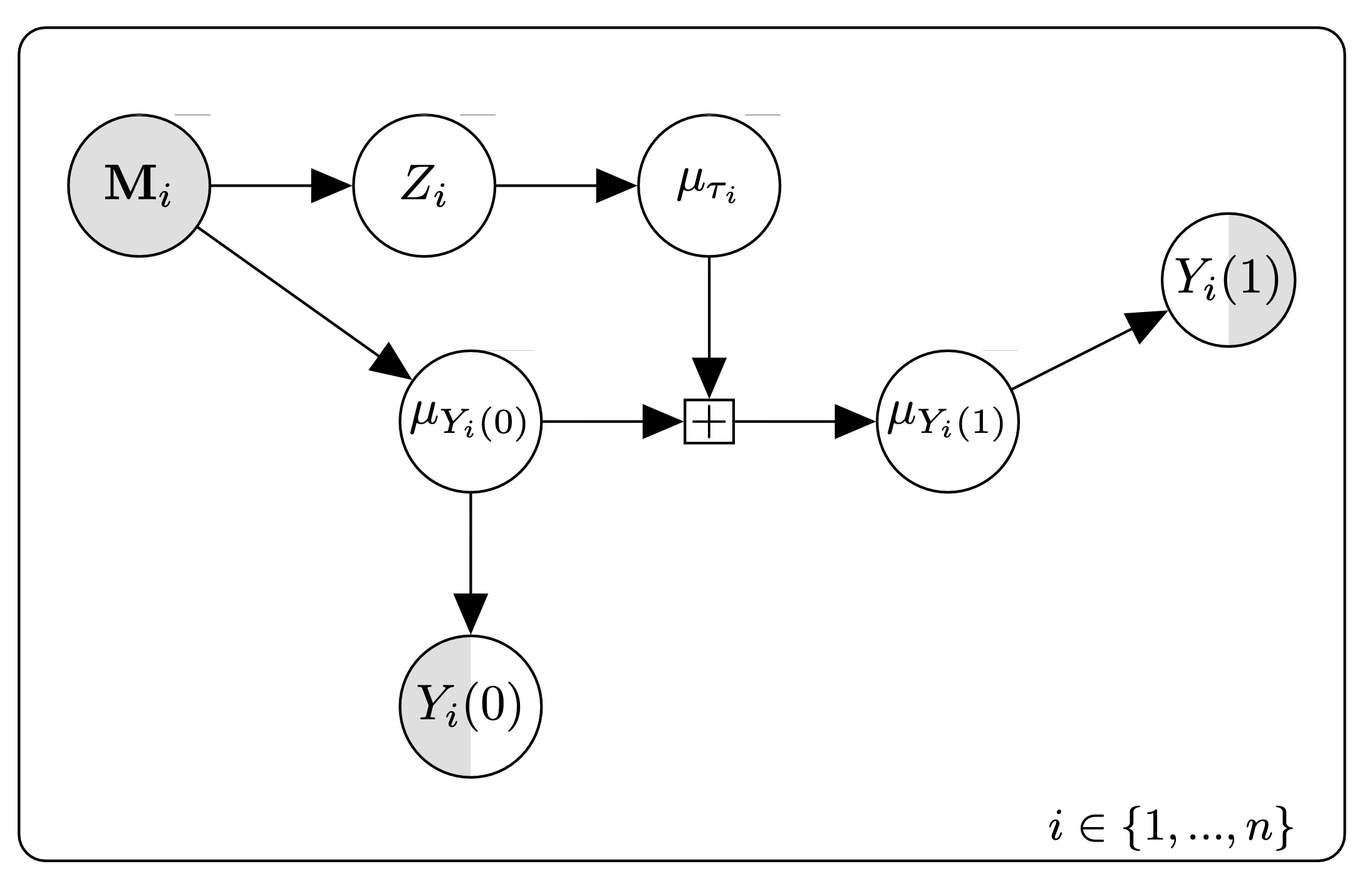
Figure 1: A stylized schematic depiction of the probabilistic treatment heterogeneity model for images. Gray circles denote observed random variables; white circles denote latent variables. Mixed gray/white nodes denote partially observed nodes (i.e., nodes observed for some, but not all, units). Square nodes denote deterministic transformations. $Z_{i}$ denotes the image type generating a distribution over treatment effects. Arrows denote statistical (not causal) dependencies.

3.3 Determination of Salience Regions in the Posterior Mean Probabilities

One benefit of the Bayesian image-type heterogeneity model is that we can examine the model in order to assess how image information translates into the predicted effect cluster. In particular, we can take the derivative of the posterior mean cluster probabilities with respect to pixel $(w,h)$: s_whk^Direction = ∑_c=1^C ∂ E[Pr(Zi= k ∣Mi=m)]∂ mwhc, where $c\in\{1,...,C\}$ denotes the channel (band) dimension. The quantity, $s_{whk}$ is a scalar summary of how changing pixel $(w,h)$ would induce changes in the predicted effect cluster probability. Because the modeling strategy is probabilistic, the salience must average over the randomness in the predicted cluster probabilities, hence the expectation on the inside of the derivative. This expectation is approximated via Monte Carlo. Positive values of this quantity would indicate that increasing the pixel intensity at $(w,h)$ would increase the probability of cluster $k$; with the same logic, negative values indicate that increasing pixel intensity at $(w,h)$ would decrease the probability of cluster $k$.

Because directional salience may not be interpretable when increasing the pixel intensity is not itself interpretable, we can also consider an approach based on magnitudes, bypassing the potentially difficult interpretation of pixel intensities in different bands: s_whk^Magnitude = ∑_c=1^C (∂ E[Pr(Zi= k ∣Mi=m)]∂ mwhc)^2. Large values of $s_{whk}^{\textrm{Magnitude}}$ reveal locations in the image that, if changed, would lead to large changes in cluster $k$ probabilities. This measure is agnostic about whether those changes would be associated with increases or decreases in those expected probabilities. This salience information is difficult to compute for post-hoc clustering methods, as the clustering of the $\hat{\tau}_{i}$’s needs to solve a second optimization problem (as in $k$-means) through which gradients with respect to the initial outcome model(s) may not be efficiently traced. Moreover, in contrast to the post-hoc approach of §LABEL:s:BaselineModel, the salience measure here incorporates uncertainty in the cluster prediction itself (since the salience averages over randomness in the cluster probabilities).

3.4 Policy Action Using the Image-based Heterogeneity Model

A major motivation for considering satellite-image-based CATEs is that we can readily generate predictive distributions over treatment effects for contexts outside the experimental setting and where no tabular covariates were measured by researchers—a possibility that may meaningfully expand the reach of causal analyses. In this context, for a new out-of-sample point not from the original dataset, $i^{\textrm{Out}}\in\mathcal{I}(\textrm{Out})$, we form a predictive distribution over image treatment effects using p(τ_i^Out ∣M_i^Out,  D) &= ∑_z=1^K ∫p(τ_i ∣Z_i^Out=z ;  Θ=θ) ⋅p(Z_i^Out=z ∣M_i^Out;  Θ=θ) ⋅p(Θ=θ∣D)  d θ We can use the predictive distribution over treatment effects to improve treatment targeting for out-of-sample individuals. With a fixed treatment budget of size $n_{1}^{O}$ for the new dataset of size $n^{O}=|\mathcal{I}(\textrm{Out})|$, this policy can be written as $\boldsymbol{\Pi}(\{\mathbf{M}_{i^{\textrm{Out}}}\}_{\mathcal{I}(\textrm{Out})})\to\{0,1\}^{n^{O}}$. There are many approaches to this problem, and we refer readers to the relevant literature (Hitsch and Misra, 2018).

3.5 Multi-modal Learning with Image and Tabular Heterogeneity

Tabular information can be readily incorporated into this modeling pipeline. For example, tabular covariates can be appended to the input of the dense part of the cluster type and baseline outcome models. The resulting treatment effect heterogeneity clusters are therefore conditional on both individual-level and also image-context-level information. This image and tabular data integration can be useful when investigators are focused on understanding the holistic heterogeneity dynamic in an experimental context, integrating both individual- and neighborhood-level information. Such a combined approach, an example of multi-modal learning (Ullah et al., 2022), can also be potentially useful in the medical domain, where image and high-dimensional medical records text can form the basis for improved patient response modeling.

3.6 Distinguishing Image from Tabular Heterogeneity

When tabular covariates were not measured or when we aim to generate predictions for observations having no measured tabular covariates, it may be useful to perform image-type effect clustering directly using images alone. When other tabular covariates are measured for the experimental sample, researchers may seek to understand the heterogeneity stemming from image information that is unique when compared with tabular covariates.

For example, information about economic class is embedded in earth observation images, since the urban poor are often concentrated in dense city centers while the affluent often live in green-space-rich areas outside cities (Venter et al., 2020). We may wonder about the remaining heterogeneity after accounting for tabular variables such as income. In this context, we can perform the image clustering on the orthogonalized outcomes: $Y_{i}(t)^{\perp}=Y_{i}(t)-\widehat{\mathbb{E}}[Y_{i}(t)|\mathbf{X}_{i}]$. The resulting clusters can then be interpreted as image effect types after accounting for the additive heterogeneity from measured tabular data. This image-specific decomposition can be helpful when geographic or neighborhood information is the focus of study.

4 Treatment Effect Cluster Recovery in Simulation

We now explore the dynamics of the proposed methods in simulation, where true treatment effects are known. We generate image-based treatment effect heterogeneity using,

$$H_{i}=\textrm{GN}(\textrm{max}(f_{l}(\mathbf{M}_{i}))),\qquad H_{i}^{+}=\underbrace{|\min\{H_{i}\}_{i=1}^{n}|}_{\color[rgb]{0,0,0}\textrm{Ensures $\tau_{i}>0$}}+\underbrace{\textrm{sign}(H_{i})\cdot|H_{i}|^{1/\gamma}}_{{\color[rgb]{0,0,0}\textrm{Generates bimodality as $\gamma\to\infty$}}}$$ (3)

where $f_{l}(\cdot)$ denotes the application of a $l\times l$ filter to the image, max($\cdot$) denotes the global maximum operation across the image, and $\textrm{GN}(\cdot)$ denotes a global normalization function scaling the $H_{i}$ values to have mean 0 and variance 1 across the image pool. The specific transformation generating $H_{i}^{+}$ is selected to ensure all the treatment effects are in the same direction (i.e., all positive) and to generate heterogeneity in the effect distribution, with greater bimodality in the treatment response as $\gamma\to\infty$. We let $\gamma=2$. We define the treatment and outcome: T_i ∼Binomial(0.5), & Y_i = T_i H_i^+ + ϵ_i, with $\epsilon_{i}\sim\mathcal{N}(0,\ \nu\cdot\textrm{Var}(H_{i}^{+}))$. The value of $\nu$ controls the extent to which the image is predictive of the outcomes, where smaller values indicate a stronger image heterogeneity signal. To explore the effect of the signal-to-noise ratio, we vary $\nu\in\{0.01,0.1,1\}$.

The filter used in the convolution function of Equation 3 is visualized in Figure LABEL:fig:SimIll, along with high and low responders from the set of images used in the simulation that we take from Landsat mosaics of sub-Saharan Africa. We have some degree of model misspecification here, as the way the data are generated is distinct from the estimation models; given this, we will examine the degree to which the various models will recover key properties of the image-based causal system.

Cluster Recovery Measure   We compare the estimated effect clustering with an oracle baseline from the true, in practice unknown, $\tau_{i}$’s. That is, we first compute the oracle $k$-means clustering: τ(z)_Oracle = $z^{\textrm{th}}$ center from the oracle $k$-means applied to the true (in practice unknown) $\tau_{i}$’s The clustering quality measure then compares the oracle with estimated cluster means: Cluster Recovery $R^{2}$   &=   1 - ∑z=1Kminz’(^τ(z) - τ(z’)Oracle)2∑z”=1K(τ(z”)Oracle- ¯τOracle)2, where $\overline{\tau}_{\textrm{Oracle}}$ denotes the mean across the oracle cluster centers. This measure is equivalent to the $R^{2}$ in predicting the oracle cluster means from the estimated ones, where the ordering of the clusters has been arranged so that each oracle center is compared to its nearest estimated counterpart.

Simulation Results   We see in the left panel of Figure 2 one representative posterior distribution over $Y_{i}(1)-Y_{i}(0)$ given estimated cluster information. We find that the estimated clusters capture the bimodality present in the true distribution of $\tau_{i}$’s. The right panel shows how the cluster recovery measure for the Image-Type Differential Effects Model and TARNet post-hoc clustering are similar in the low residual variance setting. In the high residual variance setting, the TARNet clustering struggles somewhat in recovering the oracle cluster centers. In contrast, the parsimonious Image-Type Effect Clustering Model performs best at recovering the clustering of the treatment effects across the noise range. This is encouraging for the application of the Image-Type Effect Cluster Model in practice, as presumably, the signal-to-noise ratio for real tasks involving earth observation images is relatively high.

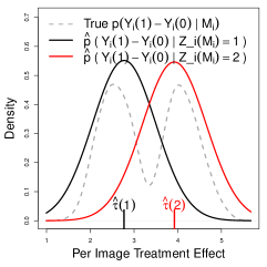
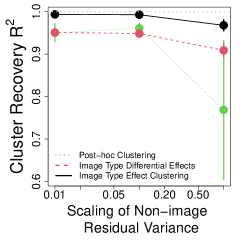
Figure 2: Left: Capturing the treatment effect heterogeneity with our Image-Type Effect Model. Right: Comparing models as we vary the signal-to-noise ratio.

5 Application to an Anti-Poverty Experiment in Uganda

Data   In our application, we explore the effects of the anti-poverty experiment performed in Uganda and described in §LABEL:s:intro. The treatment variable is the random assignment of small teams to receive grants for business ventures. The outcome variable is an aggregate summary of skilled labor (see LABEL:ss:AppOutcome) measured at the end of the experiment (two years after treatment assignment). De-identified outcome and treatment data were given voluntarily by subjects and are available under CC0 1.0 license. Longitude/latitude information about respondents’ villages is found using OpenStreetMap.

Pre-treatment image data are taken from Landsat. We use the Orthorectified ETM+ pan-sharpened data product, processed to contain minimal cloud cover. Reflectance is measured in the green, near-infrared, and short-wave infrared bands. These bands are useful in capturing information about peak vegetation, water content, and thermal dynamics, in addition to structural land features.

Empirical Results   Due to space constraints, we focus on results from the Image-Type Effect Cluster Model (details in §LABEL:ss:ImplementationDetails). We set the cluster number to 2 after finding that cluster probabilities become highly correlated with additional clusters. The top three rows in the left panel of Figure 3 show results for the highest images having the highest posterior mean probabilities for cluster 1. For each image, this figure visualizes the salience measures defined in §3.3. The bottom portion shows results for the highest posterior mean cluster 2 images. The effect for cluster 1 is substantially different than for cluster 2. Visually, we see that smaller effects exist for places with harsher terrain and less developed transportation networks, hampering economic growth. These low responders are found in the harsh mountainous northern part of Uganda. This is logical, as skilled labor tends to thrive in areas that are connected via transportation networks (Ashraf and Galor, 2011).

We show in the right panel of Figure 3 how the results of the experiment may be generalized to the entire country of Uganda, assuming no systematic bias in places chosen conditional on the image information. In particular, we show the posterior predictive mean cluster 2 probability for the entire country. This kind of analysis can provide policymakers with potentially useful information for how to improve the targeting of treatments in the future across larger geographic contexts.

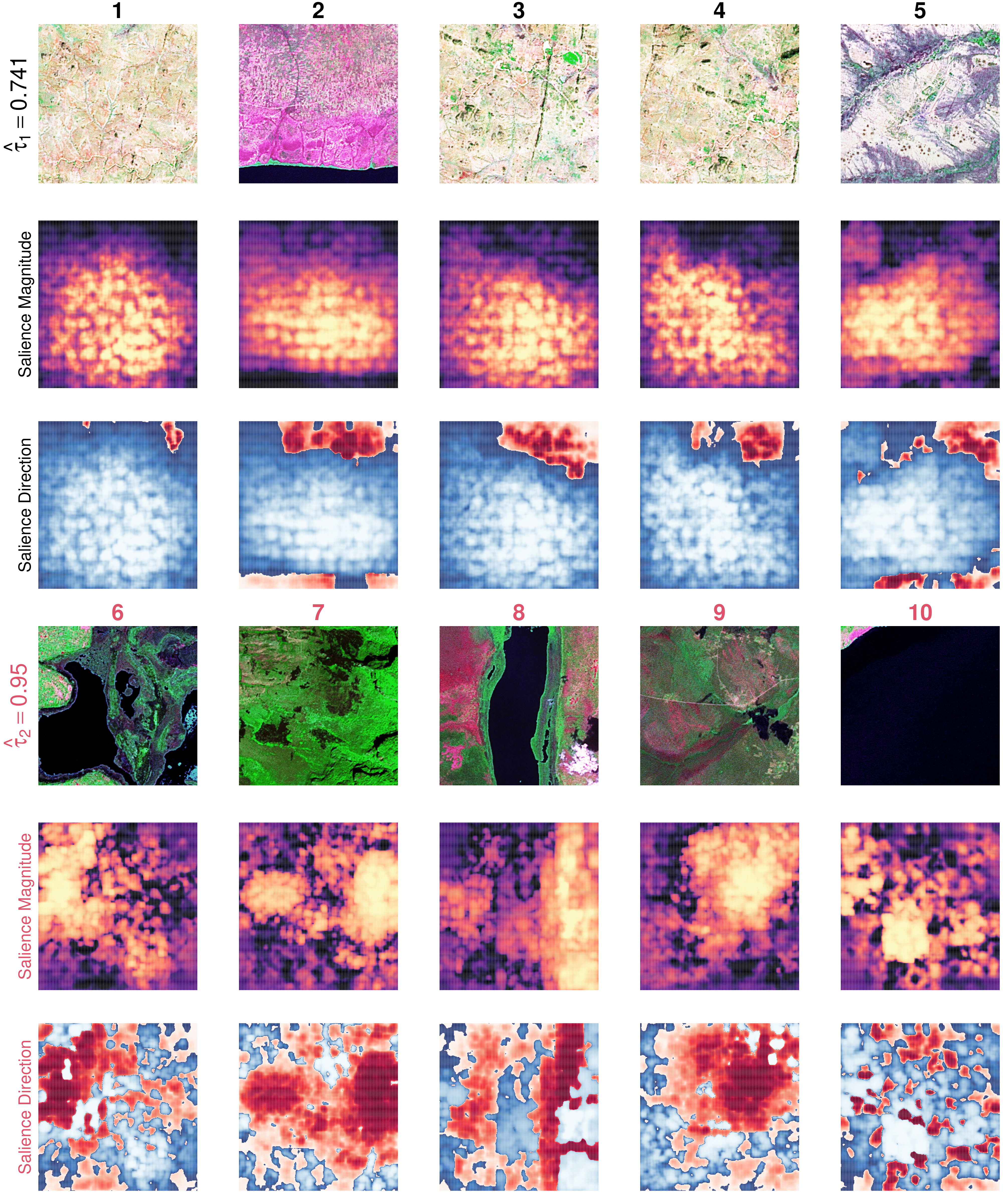
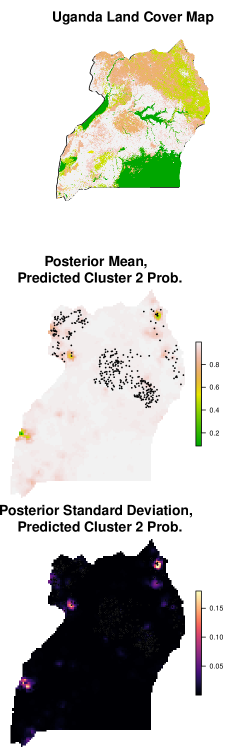
Figure 3: Left, top 3 rows: High probability cluster 1 images. Left, bottom 3 rows: High probability cluster 2 images. “Salience Magnitude” and “Direction” are defined in §3.3. Right, top: A land use map of Uganda. Right, center: Posterior predictive mean cluster 2 probabilities for the entire country. Black circles represent observed sample points. Right, bottom. Posterior standard deviation of the cluster 2 probabilities.

The Appendix contains supplementary analyses. For example, we show in Figure LABEL:fig:XMCor the correlation between the estimated Image CATEs and Tabular CATEs using various conditioning sets, as well as, in Table LABEL:tab:CorTab, between the cluster probabilities and other individual-level covariates. We show in Figure LABEL:fig:UncertainImages the images having the greatest uncertainty in the cluster probabilities (estimated by the posterior standard deviation). In §LABEL:ss:OrthoEmpirical, we orthogonalize the potential outcomes using tabular information, and the results remain similar: the correlation between raw and non-orthogonalized cluster probabilities is 0.85. Because our results remain similar after orthogonalization, the satellite images seem to supply independent and thought-provoking information about effect heterogeneity.

6 Discussion and Conclusion

Scientists and policymakers use RCTs to estimate population-wide effects (ATE) and sub-population effects (CATE), using tabular data collected at baseline, often near-time to when the RCT is launched. However, these near-time variables tend to miss important historical or neighborhood-level features. While such features are often unavailable or expensive to collect, satellite images are a data stream that captures such characteristics in an unstructured form. As no CATE method exists explicitly for image analysis, this paper presents principles and modeling strategies for analyzing image-based CATE using probabilistic image-type models. After deriving some model properties, we perform approximate inference using variational methods. Dynamics are explored via simulation; an anti-poverty field experiment from Uganda is analyzed, where we seem to find interesting heterogeneity.

Our approach has limitations, which serve to motivate future research. First, our models estimate heterogeneity clusters at the image level, but not explicitly for smaller segments of an image. Having such within-image heterogeneity segmentation would further improve understanding of what in the image is generating heterogeneity. Second, our methods estimate heterogeneity with respect to a fixed baseline (i.e., the control intervention). While the choice of baseline is clear in most settings, in unclear cases, investigators may need to explore different baselines and compare results. Third, our model is tailored for RCTs (i.e., assuming unconfoundedness); more research is required to adapt it for observational settings. Using experimental data, effect estimates are confounding-free by design; heterogeneity can be studied independently of identification. Observational data are more plentiful but require adjustment (Rosenbaum et al., 2010). We have also viewed images from solely the perspective of surrogate effect modification (in the language of Miguel and Robins (2020)); the use of images as causal modifiers or mediators is left for future study.

Finally, our focus on CATE for images opens exciting possibilities. It not only encourages others to start incorporating satellite images in their planned experiments but also reanalyze past experiments, potentially unraveling previously undetected yet significant sources of effect heterogeneity. As demonstrated in our analysis of the Ugandan anti-poverty experiment, our method identifies heterogeneity not initially detected by incorporating informative satellite data. Thus, our image-based methods have the potential to contribute to policy by complementing traditional RCT heterogeneity analysis based on tabular $\mathbf{X}_{i}$—and to analyses in other fields such as agriculture, disaster relief, climate science, and medicine where image data are also prevalent. $\square$

7 Acknowledgements

The authors thank James Bailie, Cindy Conlin, Devdatt Dubhashi, Felipe Jordan, Mohammad Kakooei, Eagon Meng, Xiao-Li Meng, Markus Pettersson, as well as seminar participants at the Causal Data Science Meeting, Texas Methods Workshop, and RAND CCI Symposium for valuable feedback on this project. We also thank Xiaolong Yang for excellent research assistance.

Appendix

A.1.1 Open-source Software & Reproducability

We make the modeling strategies introduced in this paper accessible in an open-source software package available at github.com/cjerzak/causalimages-software. For an up-to-date tutorial regarding package use, see github.com/cjerzak/causalimages-software#readme. Replication data for the experiment analyzed in the application are contained in this GitHub repository as well (we include both the experimental data from the original investigators and the geo-referenced satellite images).

A.1.2 Supplementary Information for the Image-Type Probabilistic Models

A.1.2.1 Deriving the Conditional Distribution, $\{\tau_{i}=Y_{i}(1)-Y_{i}(0)|Z_{i}=z\}$

Using the model outlined in the main text, conditioning on $\tau_{i}$, and exploiting Normality, { Y_i(1) - Y_i(0) ∣Z

References

- Ashraf and Galor [2011] Quamrul Ashraf and Oded Galor. Cultural diversity, geographical isolation, and the origin of the wealth of nations. Technical report, National Bureau of Economic Research, 2011.
- Athey and Imbens [2016] Susan Athey and Guido Imbens. Recursive partitioning for heterogeneous causal effects. Proceedings of the National Academy of Sciences, 113(27):7353–7360, 2016.
- Athey et al. [2019] Susan Athey, Julie Tibshirani, and Stefan Wager. Generalized random forests. The Annals of Statistics, 47(2):1148–1178, 2019.
- Balgi et al. [2022] Sourabh Balgi, Jose M. Pena, and Adel Daoud. Personalized Public Policy Analysis in Social Sciences using Causal-Graphical Normalizing Flows. Association for the Advancement of Artificial Intelligence: AI for Social Impact track, February 2022. URL http://arxiv.org/abs/2202.03281. arXiv: 2202.03281.
- Banerjee et al. [2011] Abhijit Banerjee, Abhijit V Banerjee, and Esther Duflo. Poor economics: A radical rethinking of the way to fight global poverty. Public Affairs, 2011.
- Blattman et al. [2014] Christopher Blattman, Nathan Fiala, and Sebastian Martinez. Generating skilled self-employment in developing countries: Experimental evidence from uganda. The Quarterly Journal of Economics, 129(2):697–752, 2014.
- Burke et al. [2021] Marshall Burke, Anne Driscoll, David B. Lobell, and Stefano Ermon. Using satellite imagery to understand and promote sustainable development. Science, 371(6535):eabe8628, March 2021. ISSN 0036-8075, 1095-9203. 10.1126/science.abe8628. URL https://www.sciencemag.org/lookup/doi/10.1126/science.abe8628.
- Castro et al. [2020] Daniel C. Castro, Ian Walker, Ben Glocker, Ian Walker, and Ben Glocker. Causality matters in medical imaging. Nature Communications, 11(1):3673, July 2020. ISSN 2041-1723. 10.1038/s41467-020-17478-w. URL https://www.nature.com/articles/s41467-020-17478-w.
- Chalupka et al. [2015] Krzysztof Chalupka, Pietro Perona, and Frederick Eberhardt. Visual Causal Feature Learning. Technical Report arXiv:1412.2309, arXiv, June 2015. URL http://arxiv.org/abs/1412.2309. arXiv:1412.2309 [cs, stat] type: article.
- Chalupka et al. [2016a] Krzysztof Chalupka, Tobias Bischoff, Pietro Perona, and Frederick Eberhardt. Unsupervised Discovery of El Nino Using Causal Feature Learning on Microlevel Climate Data. Technical Report arXiv:1605.09370, arXiv, May 2016a. URL http://arxiv.org/abs/1605.09370.
- Chalupka et al. [2016b] Krzysztof Chalupka, Frederick Eberhardt, and Pietro Perona. Multi-Level Cause-Effect Systems. In Proceedings of the 19th International Conference on Artificial Intelligence and Statistics, pages 361–369. PMLR, May 2016b. URL https://proceedings.mlr.press/v51/chalupka16.html. ISSN: 1938-7228.
- Cowan [2010] Nelson Cowan. The magical mystery four: How is working memory capacity limited, and why? Current directions in psychological science, 19(1):51–57, 2010.
- Daoud and Dubhashi [2020] Adel Daoud and Devdatt Dubhashi. Statistical modeling: the three cultures. arXiv:2012.04570 [cs, stat], December 2020. URL http://arxiv.org/abs/2012.04570. arXiv: 2012.04570.
- Daoud and Johansson [2019] Adel Daoud and Fredrik Johansson. Estimating treatment heterogeneity of international monetary fund programs on child poverty with generalized random forest. 2019.
- Daoud et al. [2021] Adel Daoud, Felipe Jordan, Makkunda Sharma, Fredrik Johansson, Devdatt Dubhashi, Sourabh Paul, and Subhashis Banerjee. Using satellites and artificial intelligence to measure health and material-living standards in India. Technical Report arXiv:2202.00109, arXiv, December 2021. URL http://arxiv.org/abs/2202.00109. arXiv:2202.00109 [cs, econ, q-fin] type: article.
- Ding et al. [2021] Mingyu Ding, Zhenfang Chen, Tao Du, Ping Luo, Josh Tenenbaum, and Chuang Gan. Dynamic Visual Reasoning by Learning Differentiable Physics Models from Video and Language. In Advances in Neural Information Processing Systems, volume 34, pages 887–899. Curran Associates, Inc., 2021. URL https://proceedings.neurips.cc/paper/2021/hash/07845cd9aefa6cde3f8926d25138a3a2-Abstract.html.
- Ding et al. [2016] Peng Ding, Avi Feller, and Luke Miratrix. Randomization inference for treatment effect variation. Journal of the Royal Statistical Society: Series B (Statistical Methodology), 78(3):655–671, 2016.
- Foulds and Frank [2010] James Foulds and Eibe Frank. A review of multi-instance learning assumptions. The knowledge engineering review, 25(1):1–25, 2010.
- Goplerud et al. [2022] Max Goplerud, Kosuke Imai, and Nicole E Pashley. Estimating heterogeneous causal effects of high-dimensional treatments: Application to conjoint analysis. arXiv preprint arXiv:2201.01357, 2022.
- Greenland et al. [2020] Sander Greenland, Michael P Fay, Erica H Brittain, Joanna H Shih, Dean A Follmann, Erin E Gabriel, and James M Robins. On causal inferences for personalized medicine: How hidden causal assumptions led to erroneous causal claims about the d-value. The American Statistician, 74(3):243–248, 2020.
- Hitsch and Misra [2018] Günter J Hitsch and Sanjog Misra. Heterogeneous treatment effects and optimal targeting policy evaluation. Available at SSRN 3111957, 2018.
- Imai and Ratkovic [2013] Kosuke Imai and Marc Ratkovic. Estimating treatment effect heterogeneity in randomized program evaluation. The Annals of Applied Statistics, 7(1):443–470, 2013.
- Jerzak et al. [2023] Connor T Jerzak, Fredrik Johansson, and Adel Daoud. Integrating earth observation data into causal inference: Challenges and opportunities. arXiv preprint arXiv:2301.12985, 2023.
- Kaddour et al. [2021a] Jean Kaddour, Yuchen Zhu, Qi Liu, Matt J Kusner, and Ricardo Silva. Causal effect inference for structured treatments. Advances in Neural Information Processing Systems, 34, 2021a.
- Kaddour et al. [2021b] Jean Kaddour, Yuchen Zhu, Qi Liu, Matt J. Kusner, and Ricardo Silva. Causal Effect Inference for Structured Treatments. Advances in Neural Information Processing Systems, 34, 2021b.
- Kallus [2020] Nathan Kallus. Deepmatch: Balancing deep covariate representations for causal inference using adversarial training. In International Conference on Machine Learning, pages 5067–5077. PMLR, 2020.
- Kino et al. [2021] Shiho Kino, Yu-Tien Hsu, Koichiro Shiba, Yung-Shin Chien, Carol Mita, Ichiro Kawachi, and Adel Daoud. A scoping review on the use of machine learning in research on social determinants of health: Trends and research prospects. SSM - Population Health, 15:100836, September 2021. ISSN 2352-8273. 10.1016/j.ssmph.2021.100836. URL https://www.sciencedirect.com/science/article/pii/S2352827321001117.
- Krishnan et al. [2020] Ranganath Krishnan, Mahesh Subedar, and Omesh Tickoo. Specifying weight priors in bayesian deep neural networks with empirical bayes. In Proceedings of the AAAI Conference on Artificial Intelligence, volume 34, pages 4477–4484, 2020.
- Künzel et al. [2019] Sören R Künzel, Jasjeet S Sekhon, Peter J Bickel, and Bin Yu. Metalearners for estimating heterogeneous treatment effects using machine learning. Proceedings of the national academy of sciences, 116(10):4156–4165, 2019.
- Lopez-Paz et al. [2017] David Lopez-Paz, Robert Nishihara, Soumith Chintala, Bernhard Scholkopf, and Leon Bottou. Discovering Causal Signals in Images. pages 6979–6987, 2017. URL https://openaccess.thecvf.com/content_cvpr_2017/html/Lopez-Paz_Discovering_Causal_Signals_CVPR_2017_paper.html.
- Louizos et al. [2017] Christos Louizos, Uri Shalit, Joris M Mooij, David Sontag, Richard Zemel, and Max Welling. Causal Effect Inference with Deep Latent-Variable Models. In Advances in Neural Information Processing Systems, volume 30. Curran Associates, Inc., 2017. URL https://proceedings.neurips.cc/paper/2017/hash/94b5bde6de888ddf9cde6748ad2523d1-Abstract.html.
- Luedtke and van der Laan [2016] Alexander R Luedtke and Mark J van der Laan. Super-learning of an optimal dynamic treatment rule. The international journal of biostatistics, 12(1):305–332, 2016.
- Miguel and Robins [2020] Hernán Miguel and Jamie Robins. Causal Inference: What If. Boca Raton: Chapman & Hall/CRC, 2020.
- Nie and Wager [2021] Xinkun Nie and Stefan Wager. Quasi-oracle estimation of heterogeneous treatment effects. Biometrika, 108(2):299–319, 2021.
- Paciorek [2010] Christopher J Paciorek. The importance of scale for spatial-confounding bias and precision of spatial regression estimators. Statistical science: a review journal of the Institute of Mathematical Statistics, 25(1):107, 2010.
- Parmas and Sugiyama [2021] Paavo Parmas and Masashi Sugiyama. A unified view of likelihood ratio and reparameterization gradients. In International Conference on Artificial Intelligence and Statistics, pages 4078–4086. PMLR, 2021.
- Pawlowski et al. [2020] Nick Pawlowski, Daniel C. Castro, and Ben Glocker. Deep Structural Causal Models for Tractable Counterfactual Inference. arXiv:2006.06485 [cs, stat], October 2020. URL http://arxiv.org/abs/2006.06485. arXiv: 2006.06485.
- Pearl [2009] Judea Pearl. Causality. Cambridge university press, 2009.
- Pearl and Bareinboim [2022] Judea Pearl and Elias Bareinboim. External validity: From do-calculus to transportability across populations. In Probabilistic and Causal Inference: The Works of Judea Pearl, pages 451–482. 2022.
- Ramachandra [2019] Vikas Ramachandra. Causal inference for climate change events from satellite image time series using computer vision and deep learning. arXiv preprint arXiv:1910.11492, 2019.
- Ranganath et al. [2014] Rajesh Ranganath, Sean Gerrish, and David Blei. Black box variational inference. In Artificial intelligence and statistics, pages 814–822. PMLR, 2014.
- Rosenbaum et al. [2010] Paul R Rosenbaum, PR Rosenbaum, and Briskman. Design of observational studies, volume 10. Springer, 2010.
- Rubin [2005] Donald B Rubin. Causal inference using potential outcomes: Design, modeling, decisions. Journal of the American Statistical Association, 100(469):322–331, 2005.
- Schölkopf et al. [2021] Bernhard Schölkopf, Francesco Locatello, Stefan Bauer, Nan Rosemary Ke, Nal Kalchbrenner, Anirudh Goyal, and Yoshua Bengio. Towards Causal Representation Learning. arXiv:2102.11107 [cs], February 2021. URL http://arxiv.org/abs/2102.11107. arXiv: 2102.11107.
- Shalit et al. [2017] Uri Shalit, Fredrik D Johansson, and David Sontag. Estimating individual treatment effect: generalization bounds and algorithms. In International Conference on Machine Learning, pages 3076–3085. PMLR, 2017.
- Shiba et al. [2021] Koichiro Shiba, Adel Daoud, Hiroyuki Hikichi, Aki Yazawa, Jun Aida, Katsunori Kondo, and Ichiro Kawachi. Heterogeneity in cognitive disability after a major disaster: A natural experiment study. Science advances, 7(40):eabj2610, 2021.
- Ullah et al. [2022] Ubaid Ullah, Jeong-Sik Lee, Chang-Hyeon An, Hyeonjin Lee, Su-Yeong Park, Rock-Hyun Baek, and Hyun-Chul Choi. A review of multi-modal learning from the text-guided visual processing viewpoint. Sensors, 22(18):6816, 2022.
- Venter et al. [2020] Zander S Venter, Charlie M Shackleton, Francini Van Staden, Odirilwe Selomane, and Vanessa A Masterson. Green apartheid: Urban green infrastructure remains unequally distributed across income and race geographies in south africa. Landscape and Urban Planning, 203:103889, 2020.
- Wen et al. [2018] Yeming Wen, Paul Vicol, Jimmy Ba, Dustin Tran, and Roger Grosse. Flipout: Efficient pseudo-independent weight perturbations on mini-batches. arXiv preprint arXiv:1803.04386, 2018.
- Westling and McCormick [2019] T Westling and TH McCormick. Beyond prediction: A framework for inference with variational approximations in mixture models. Journal of Computational and Graphical Statistics, 28(4):778–789, 2019.
- Yi et al. [2020] Kexin Yi, Chuang Gan, Yunzhu Li, Pushmeet Kohli, Jiajun Wu, Antonio Torralba, and Joshua B. Tenenbaum. CLEVRER: CoLlision Events for Video REpresentation and Reasoning. Technical Report arXiv:1910.01442, arXiv, March 2020. URL http://arxiv.org/abs/1910.01442. arXiv:1910.01442 [cs] type: article.
- Zhao et al. [2017] Qingyuan Zhao, Dylan S Small, and Ashkan Ertefaie. Selective inference for effect modification via the lasso. arXiv preprint arXiv:1705.08020, 2017.