Characterization of variational quantum algorithms using free fermions

Abstract

We study variational quantum algorithms from the perspective of free fermions. By deriving the explicit structure of the associated Lie algebras, we show that the Quantum Approximate Optimization Algorithm (QAOA) on a one-dimensional lattice – with and without decoupled angles – is able to prepare all fermionic Gaussian states respecting the symmetries of the circuit. Leveraging these results, we numerically study the interplay between these symmetries and the locality of the target state, and find that an absence of symmetries makes nonlocal states easier to prepare. An efficient classical simulation of Gaussian states, with system sizes up to $80$ and deep circuits, is employed to study the behavior of the circuit when it is overparameterized. In this regime of optimization, we find that the number of iterations to converge to the solution scales linearly with system size. Moreover, we observe that the number of iterations to converge to the solution decreases exponentially with the depth of the circuit, until it saturates at a depth which is quadratic in system size. Finally, we conclude that the improvement in the optimization can be explained in terms of better local linear approximations provided by the gradients.

1 Introduction

Variational quantum algorithms have recently received much attention as a potential candidate for demonstrating quantum advantage. Originally proposed in the context of quantum chemistry [76] and classical optimization problems [28], such algorithms have since found wide use as a tool for leveraging the current generation of noisy, intermediate scale quantum computers [77] to tackle problems which are hard to solve classically. For that purpose they have been extended to a myriad of domains, including machine learning, [27, 38, 9, 1, 81, 18], preparation of general condensed matter quantum states [41, 105, 29, 79, 80, 101, 46], finance [71, 25], molecular biology and biochemisty [10, 74], and linear algebra [11, 17, 106], and have been implemented in numerous quantum simulation platforms [48, 34, 75, 5, 102].

A major issue with this class of algorithms is that they are notoriously hard to optimize classically. Not only are they known to have an optimization landscape riddled with local minima [44, 58], they also suffer from the phenomenon of “barren plateaus", in which the gradients with respect to the optimization parameters vanish exponentially with system size [99, 63]. Though several strategies have been proposed to deal with this problem [56, 90, 52, 110, 57, 35, 64] it remains an active area of research.

Successfully employing parametrized circuits requires a balance between expressibility and trainability. Indeed, while universal circuit ansätze exist [66, 8], problem-agnostic circuits typically present barren plateaus [43]. Thus, it is crucial to design parameterized circuits that are able to adequately prepare or approximate the quantum state of interest, while not being overly expressive so as not to compromise its trainability. To this end, a characterization of the expressibility of these algorithms has been performed in several contexts, and strategies to systematically quantify it have been proposed [23, 84, 68, 1, 2]. A way to constrain the expressibility of a parameterized circuit is to employ problem-tailored ansätze, such as the Hamiltonian Variational Ansatz [103], among other strategies such as exploiting symmetries in the problem [33, 98, 95, 26, 59] or removing redundant parameters [31, 32].

Other factors not immediately linked to the expressibility of the circuit are known to affect the optimization, such as the boundary conditions used; these have been observed to greatly affect the success of optimization, and strategies have recently been proposed to address this issue [86]. Another set of such factors is related to the individual characteristics of states to be prepared, such as locality of correlations and entanglement [42, 60, 94, 96, 93, 20]. Despite the extensive work done on this subject, there is no systematic characterization or theory explaining the interplay between all these aspects and their connection to expressibility.

Finally, it has been observed that an increase in the number of parameters in the circuit without a corresponding increase in the expressibility induces an overparameterized regime, where the optimization is known to converge significantly faster, becoming less prone to local minima and alleviating the aforementioned issues [49, 50, 53, 54]. Though significant progress in explaining the mechanism behind this phenomenon has been achieved [108, 54], open questions remain, such as how to determine the optimal circuit depth that best leverages this effect.

In this work, we begin by comprehensively characterizing the original QAOA protocol [28] on a 1D lattice and a variation on it using decoupled angles [40]. By deriving the explicit structure of the associated Lie algebras [54, 66], we show that it can prepare exactly all fermionic Gaussian states satisfying the symmetries of the circuit. Guided by these results, we find that, while decoupling the angles increases the number of parameters and the expressibility of the circuit by removing symmetries, this makes the preparation of non-local states easier and of local states harder, flipping the behavior observed when these angles are coupled. This contrasts with the commonly held belief that the use of symmetries is beneficial to the optimization [6, 33, 55, 65, 73, 82, 83, 109, 92].

By leveraging covariance matrix and automatic differentiation techniques to simulate deep circuits and system sizes up to $80$ qubits, we study the overparameterized regime of optimization, exploiting the fact that its onset is polynomial in lattice size for the ansätze we consider (see [53, 54] and Section 3.1). In these conditions, we observe that the number of iterations to converge to the solution scales linearly with the size of the system. This contrasts with the polynomial scaling we encounter at smaller depths. Moreover, we quantify the degree of improvement that overparameterization confers to the optimization as the circuit depth increases. We find that the number of iterations to converge decays exponentially with circuit depth, and that the optimization hardness develops a minimum for a depth that is proportional to $L^{2}$, the square of the system size. Finally, we find that the exponential convergence to the solution seen in the overparameterized regime can be explained in terms of an improvement of the quality of the linear approximations provided by the gradients, elucidating why the optimization hardness continues to decrease even after local minima disappear.

This paper is organized as follows. In Sec. 2 we introduce the variational setup, focusing on free-fermion systems, and establish the associated notation. Moreover, we develop Lie theoretical tools for the analysis of variational algorithms. We apply these tools in Sec. 3 which contains our main results. In particular, Section 3.1 characterizes the expressibility of protocols introduced in Section 2.3, where they are presented alongside a concise introduction to free fermionic systems. In Section 3.2, we explore the optimization associated to the corresponding parameterized circuits, and highlight the influence of symmetries and the locality of the target state. In Section 3.3 we discuss the effect of overparameterization, and perform a scaling of the number of iterations to converge with system size and circuit depth. Our conclusions are presented in Section 4, while the Appendixes contain further numerical characterization of the circuit’s optimization landscape in terms of gradient variance, staircase structure in optimization traces, and the details of the underlying Lie algebra structure.

2 Preliminaries

2.1 Variational Quantum Algorithms

Variational quantum algorithms (VQA) [14, 7] are generally formulated as a feedback loop between an optimization routine running on a classical computer, and a quantum simulator. This routine manipulates a set of controllable parameters defining a family quantum circuits with the objective of finding a circuit which is able to prepare a quantum state of interest (though more general definitions exist depending on the problem at hand). In this context, the parameterized family of quantum circuits we will focus on is constructed by following the alternating “bang-bang" structure of the Quantum Approximate Optimization Algorithm (QAOA) [28, 107]. Given a set of Hamiltonians $\mathcal{H}=(H_{1},...,H_{m})$, the circuit is defined by the unitary operator

$$U(\bm{\theta},p)=\exp(-i\theta_{p,m}H_{m})...\exp(-i\theta_{p,1}H_{1})$$

$$...\exp(-i\theta_{1,m}H_{m})...\exp(-i\theta_{1,1}H_{1}).$$ (1)

where $p$ controls the circuit depth and $\bm{\theta}\equiv\{\theta_{1,1},\theta_{1,2},\ldots,\theta_{p,m}\}$ are the parameters to be optimized. We call such a set of Hamiltonians $\mathcal{H}$ a protocol. The associated parameters are often called angles in the literature.

Given an initial state $\ket{\psi(0)}$ and a set of parameters $\bm{\theta}$, this circuit prepares the state

$$\ket{\psi(\bm{\theta})}=U(\bm{\theta},p)\ket{\psi(0)}.$$ (2)

The goal, as outlined above, is to employ a classical optimization routine in order to find a set of angles $\bm{\theta}^{*}$, such that $\ket{\psi(\bm{\theta}^{*})}$ is the quantum state of interest, which we call the target state. This is done by supplying the optimizer with a cost function, which measures the distance between the state in preparation and the target state.

Here, we define the target state as being the unique ground state of some quantum Hamiltonian $H$. In this case, one can use a cost function based on the expectation value of the state with respect to this Hamiltonian. We use the shifted energy density as the cost function,

$$e(\psi)=\frac{\langle\psi|H|\psi\rangle-E_{0}}{L},$$ (3)

where $E_{0}$ is the ground state energy of $H$ and $L$ is the size of the system under consideration. By the variational principle, and given that we assume that the target state is the unique ground state of $H$, this cost is minimized and is equal to zero when $\ket{\psi}$ is the target state. In what follows, we refer to the Hamiltonian featuring in this cost function as the target Hamiltonian.

2.2 Lie Theory and Expressibility

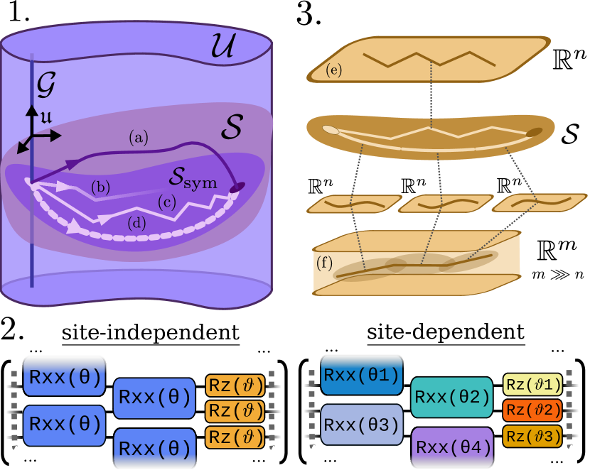
Figure 1: 1. Schematic depicting the Lie structures introduced in Section 2.2 and their relation to variational optimization. From an initial state, the set of unitaries generated by the parameterized circuit, $\mathcal{U}$, prepares a manifold of states $\mathcal{S}$. The space of directions that the protocol is able to explore at a given point is characterized by the Lie algebra $\mathfrak{u}$, and there is a redundancy in the unitaries preparing a state which is represented by a stabilizer gauge group $\mathcal{G}$. Symmetries in the protocol constrain the optimization (a) to a submanifold of states $\mathcal{S}_{\text{sym}}$, which affects the landscape by introducing local minima (b) and restricting the features available to the optimizer, causing the optimization to take longer (c), as explained in Section 3.2. By increasing the depth of the circuit, the variational protocol enters an overparameterized regime (d), where minima disappear and convergence of the cost function to a global minimum becomes exponential. 2. Circuits illustrating the variational protocols introduced in Section 2.3 and studied throughout the rest of this paper 3. The parameterization at minimal circuit depth $\hat{p}$ (e) matches the dimension of the manifold of states, so that minima exist and are unique. By the implicit function theorem, the overparameterization (f) defines local, lower-dimensional parameterizations matching the dimension of the manifold. These more adequately capture its features, while describing the optimization path in a piecewise manner (see Section 3.3). It is an open question whether a global exact parameterization with these properties could be found.

Lie theoretical techniques provide a powerful tool to characterize the expressibility of quantum controllable systems [3]. They have been previously used in the literature to prove the universality of a set of protocols under certain assumptions [66]. These have been further employed to characterize controllability and overparameterisation in variational quantum algorithms [53, 54], and have recently found use in characterizing symmetries in data in the context of machine learning [65, 55].

Here we summarize and formalize the theory behind this and define the associated notation. Given $U(\bm{\theta},p)$ defined by the Hamiltonians $\mathcal{H}=(H_{1},...,H_{m})$ as in Section 2.1, we define

$$\mathcal{U}=\bigcup_{p=1}^{\infty}\mathcal{U}^{p}, \mathcal{U}^{p}=\{U(\theta,p)\mathrel{\mathop{\mathchar 58\relax}}\theta\in\mathbb{R}^{mp}\}.$$ (4)

The set $\mathcal{U}$ contains all unitaries that the protocol $\mathcal{H}$ can generate at arbitrary circuit depth. It is a group, as it contains the product of any two of its elements and the inverse of any of its elements. Further, since matrix multiplication is differentiable, it constitutes a Lie group.

Associated to the Lie group $\mathcal{U}$ is a Lie algebra $\mathfrak{u}$, which can be defined at a point $\theta$ as

$$\mathfrak{u}=\left\{\frac{\partial U(\theta,p)}{\partial\theta_{i}}\mathrel{\mathop{\mathchar 58\relax}}i,p\in\mathbb{N}^{+}\right\}.$$ (5)

It characterizes how the circuit $U(\theta,p)$ changes with an infinitesimal variation of the parameters. Note that $\mathcal{U}=\{e^{-iH}\mathrel{\mathop{\mathchar 58\relax}}iH\in\mathfrak{u}\}$ and that $\mathfrak{u}=\langle iH_{1},...,iH_{m}\rangle$ [66, 19], where $\langle...\rangle$ denotes the Lie algebra generated by these elements i.e the space obtained by iteratively taking the Lie bracket $[A,B]=AB-BA$ of $iH_{1},...,iH_{N}$ [36].

We further define

$$\mathcal{S}^{p}=\{U(\theta,p)|\psi(0)\rangle\mathrel{\mathop{\mathchar 58\relax}}\theta\in\mathbb{R}^{mp}\}, \mathcal{S}=\bigcup_{p=1}^{\infty}\mathcal{S}^{p},$$ (6)

as the set of states preparable by the variational quantum circuit at depth $p$ and at any depth, respectively. We emphasize that $\mathcal{S}$ depends on the initial state chosen.

We will restrict our analysis to finite dimensional spaces, for which there must exist a $p^{*}$ such that $\mathcal{U}=\mathcal{U}^{p^{*}}$ [19]. By the same argument, there must be a $\hat{p}$ such that $\mathcal{S}=\mathcal{S}^{\hat{p}}$. This represents the circuit depth at which the circuit has reached maximum expressibility for a given initial state. We will see that, in general, $\hat{p}<p^{*}$. This happens because there can be a set $\mathcal{G}$ of unitary matrices in $\mathcal{U}$ that leave the initial state $\ket{\psi(0)}$ invariant, forming a stabilizer subgroup. Mathematically, this translates into $\mathcal{U}$ having a fiber bundle structure and $\mathcal{S}\cong\mathcal{U}/\mathcal{G}$, where $\mathcal{G}$ represents a Gauge symmetry group [67] (see Figure 1.1 for a graphical summary). As a consequence of this,

$$\dim\mathcal{S}=\dim\mathcal{U}-\dim\mathcal{G}$$ (7)

justifying that, in general, $\mathcal{S}$ will require less parameters to describe than $\mathcal{U}$. It is an open question whether there is a method to systematically determine $p^{*}$ and $\hat{p}$ given a set of Hamiltonians $\mathcal{H}$.

Since $\mathcal{U}=\{e^{-iA_{1}}e^{-iA_{2}}....e^{-iA_{m}}\mathrel{\mathop{\mathchar 58\relax}}m\in\mathbb{N},A_{j}\in\mathfrak{u}\}$ [66, 19], the unitaries in $\mathcal{U}$ can approximate a quantum annealing protocol and thus adiabatically prepare the ground state of any Hamiltonian in $\mathfrak{u}$ [62], provided that $\ket{\psi(0)}$ is the ground state of some $H_{0}\in\mathfrak{u}$. Conversely, if $\ket{\psi}$ is prepared by $U\in\mathcal{U}$, then it is the ground state of $H=UH_{0}U^{\dagger}\in\mathfrak{u}$. Thus, the Lie algebra $\mathfrak{u}$ fully characterizes the set $\mathcal{S}$ of preparable states; we will exploit this in Section 3.1 to study the expressibility of the protocols defined in Section 2.3.

2.3 Free fermionic systems and VQA

Throughout this paper, we work with a $1$D spin system on a linear lattice, and we denote the corresponding lattice size by $L$. We define Majorana operators through the standard Jordan-Wigner transformation

$$\gamma_{2j-1}=Z...ZX_{j}, \gamma_{2j}=Z...ZY_{j},$$ (8)

where we assume that the string of $Z$s stretches from the left end of the lattice to the $i$th position. Quadratic fermionic Hamiltonians (which we abbreviate to “quadratic Hamiltonians") are of the form

$$H=i\sum_{j,k}h_{j,k}\gamma_{j}\gamma_{k},$$ (9)

where $h_{j,k}$ is a $2L\times 2L$ real and antisymmetric matrix. Note that all quadratic Hamiltonians preserve (commute with) the fermionic parity $P=\prod_{j}Z_{j}$. The eigenstates of a quadratic Hamiltonian are fermionic Gaussian states (FGS), which are a class of quantum states that are fully determined (up to a phase) by their $2L\times 2L$ covariance matrix

$$\Gamma_{jk} =\frac{i}{2}\langle\gamma_{j}\gamma_{k}-\gamma_{k}\gamma_{j}\rangle_{\psi}$$

$$=\frac{i}{2}\operatorname*{Tr}(|\psi\rangle\langle\psi|(\gamma_{j}\gamma_{k}-\gamma_{k}\gamma_{j})),$$ (10)

which is real and antisymmetric.

Both FGS and quadratic Hamiltonians are efficiently representable, requiring a number of parameters that is quadratic in system size to be specified. Moreover, the quantum dynamics associated to the evolution of a covariance matrix under the action of a quadratic Hamiltonian is efficiently computable, as is its expectation value with respect to a quantum observable [97, 91, 88].

We now establish how symmetries in the 1D lattice are reflected on the structures we have just introduced. The covariance matrix of a translationally invariant FGS $\ket{\psi}$ and a translationally invariant quadratic Hamiltonian defined by $h_{j,k}$ satisfy, respectively:

$$\Gamma_{jk}=\Gamma_{j+2m\;k+2m}, h_{j,k}=h_{j+2m,k+2m},$$ (11)

for all integers $m$ and it is understood that coefficients are taken modulo the lattice size. The covariance matrix of a lattice inversion symmetric FGS $\psi$ and a lattice inversion symmetric quadratic Hamiltonian $H$ defined by $h_{j,k}$ satisfy, respectively:

$$\Gamma_{jk}=(-1)^{j-k+1}\Gamma_{L-k+1\;L-j+1},$$

$$h_{j,k}=(-1)^{j-k+1}h_{L-k+1\;L-j+1}$$ (12)

Throughout, we denote by “symmetric FGS" and “symmetric quadratic Hamiltonians" those that are invariant both under translation and lattice inversion.

Following the framework outlined in Section 2.1 we study two different protocols, both of which feature only quadratic Hamiltonians:

1. A site-independent protocol, defined by the set

   $$\mathcal{I} =\left(i\sum_{j}Z_{j},i\sum_{j}X_{j}X_{j+1}\right)$$

   $$=\left(-\sum_{j}\gamma_{2j-1}\gamma_{2j},-\sum_{j}\gamma_{2j}\gamma_{2j+1}\right).$$ (13)

   and we denote its Lie algebra by $\mathfrak{i}$.

2. A site dependent protocol, where

   $$\mathcal{D}=( iX_{1}X_{2},...,iX_{N-1}X_{N},$$

   $$iZ_{1},...,iZ_{N})$$

   $$=( -\gamma_{2}\gamma_{3},...,-\gamma_{N-1}\gamma_{N-2},$$

   $$-\gamma_{1}\gamma_{2},...,-\gamma_{N-1}\gamma_{N}),$$ (14)

   and we denote its Lie algebra by $\mathfrak{d}$.

The former corresponds to the original QAOA protocol [28] on a linear lattice, while the latter results from removing the layer-wise coupling in the angles of this original protocol [40]. We will see that this decoupling results in distinct properties with respect to the optimization of the associated variational algorithm.

Writing out the corresponding unitary explicitly:

$$U(p,\theta)=\exp(-i\sum_{k}\theta_{p,Z}^{k}Z_{k})\exp(-i\sum_{k}\theta_{p,XX}^{k}X_{k}X_{k+1})...\exp(-i\sum_{k}\theta_{1,Z}^{k}Z_{k})\exp(-i\sum_{k}\theta_{1,XX}^{k}X_{k}X_{k+1}).$$ (15)

As mentioned above, the site-independent protocol can be seen as the site-dependent one with the additional constraint that $\theta^{i}_{a,P}=\theta_{a,P}$, i.e., the value of the angle is the same across a circuit layer.

The full structure of the Lie algebras corresponding to the protocols above is elucidated in Appendix B. In particular, a basis for these algebras is obtained by iteratively taking the commutators of their generators. Moreover, we clarify how their structure changes when we restrict ourselves to a particular sector of the parity symmetry. In the next section, we will employ them to study the expressibility of the corresponding protocols following Section 2.2.

3 Results

3.1 Circuit expressibility and saturation

Here, we determine the expressibility of the protocols introduced in the previous section by examining the corresponding Lie algebra. In particular, we study the set of unitaries $\mathcal{U}$ that each protocol can generate and the set of states $S$ that each can prepare. In what follows we consider the initial state to be a fermionic Gaussian state of a given parity respecting the symmetries of the circuit.

Our results are summarized in Table 1. All protocols are able to prepare every FGS with the same parity as the initial state and respecting the symmetries of the circuit. This can be proved by studying the structure of the corresponding Lie algebras, derived in Appendix B and referenced in Table 1. By applying the Jordan-Wigner transformation, these Lie algebras can be seen to form the set of free fermionic Hamiltonians satisfying the symmetries of the circuit. As shown in Section 2.2, every ground state of such a Hamiltonian can be prepared by the circuit at some depth; and the set of these ground states are precisely the fermionic Gaussian states having the same parity as the initial state and respecting the appropriate symmetries.

As outlined in Section 2.2, there can be a symmetry subgroup $\mathcal{G}$ of $\mathcal{U}$ that leaves the initial state invariant. In the case of a FGS, there is a $U(L)$ freedom in the fermionic modes, which can be rotated without changing the underlying state [104]. The subset of these rotations contained in $\mathcal{U}$ will form $\mathcal{G}$; this can be all of the $U(L)$ freedom, as is the case of the site dependent protocol, or only part of it, in which case $\dim\mathcal{G}<\dim U(L)$.

We further attempt to determine the minimum depth $\hat{p}$ necessary to prepare any state in $\mathcal{S}$ for each of the cases in Table 1. In what follows, we denote by $q$ the number of variational parameters per unit of $p$. While it is clear that $q\hat{p}$ must be greater than $\dim\mathcal{S}$, the circuit must be also be deep enough so that correlations are able to propagate across the lattice [62]. A consequence of this is that $\hat{p}\geq\lceil L/2\rceil$. We compute $\hat{p}$ numerically by randomly generating Hamiltonians in $\mathfrak{u}$ and verifying that their ground states are prepared to numerical precision. The quantity

$$q\hat{p}-\dim\mathcal{S},$$ (16)

represents the number of parameters in the circuit that exceeds $\dim\mathcal{S}$.

We find, in cases where periodic boundary conditions (PBC) are employed, or where the site-dependent protocol is used, that $\hat{p}=\lceil L/2\rceil$, saturating the aforementioned lower bound. For the remaining case, which corresponds to the site-independent protocol using open boundary conditions (OBC), $\hat{p}$ proved to be unfeasible to determine numerically in a precise manner due to a significantly higher number of local minima.

In the site-independent case with periodic boundary conditions, $q\hat{p}=\dim\mathcal{S}$, which suggests an exact parameterization of $\mathcal{S}$. In contrast, in the site-dependent case with PBCs, there are $q\hat{p}-\dim\mathcal{S}=L$ redundant parameters at $\hat{p}$. One can, however, do away with them by removing the last $e^{-i\sum_{j}\theta_{p,Z}Z_{j}}$ layer from this circuit, while still being able to prepare all states in $\mathcal{S}$. Thus, in this case, one can also obtain an exact parameterization. By abuse of terminology, we will refer to the behavior at circuit depth $\hat{p}$ as the exactly parameterized regime, regardless of whether $q\hat{p}=\dim\mathcal{S}$. A consequence of having an exact parameterization of $\mathcal{S}$ is that, when the associated angles are appropriately restricted, global minima exist and are unique.

	Dependent		Independent
	OBC	PBC	OBC	PBC
$\mathcal{S}$	fixed parity FGS		fixed parity FGS satisfying (12)	fixed parity FGS satisfying (11) & (12)
$\mathfrak{u}$	(24)	(26)	(28)	(30)
$\mathfrak{u}$ (fixed parity)	(24)		(28)	(37)
$\dim\mathcal{U}$	$L(2L-1)$	$2L(2L-1)$	$L^{2}$	$3L-2$
$\dim\mathcal{U}$ (fixed parity)	$L(2L-1)$		$L^{2}$	$\lfloor 3L/2\rfloor$
$\dim\mathcal{G}$	$L^{2}$		$L(L+1)/2$	$\lfloor L/2\rfloor$
$\dim\mathcal{S}$	$L(L-1)$		$L(L-1)/2$	$L$

Table 1: Table summarizing the expressibility of the site-dependent, Eq. (1), and site-independent, Eq. (2), protocols. The structure of the Lie algebras $\mathfrak{u}$ corresponding to each protocol is given in Appendix B; the entries in this table refer to the respective basis. As outlined in the main text, these are used to analytically deduce $\mathcal{U}$, the space of unitaries that each protocol can generate, and $S$, the space of states that each protocol can prepare. We assume that the initial state is a FGS of a given parity respecting the symmetries of the circuit.

3.2 Effect of Symmetries and Locality on the Optimization Landscape

We proceed to study the hardness of the optimization and the characteristics of the associated landscape when running a variational algorithm using the site-independent, Eq. (1), and site-dependent, Eq. (2), protocols. We work with PBC, and target the ground state of two models:

1. The critical transverse field Ising model [41]

   $$H_{I}=-\sum_{j}X_{j}X_{j+1}-\sum_{j}Z_{j}.$$ (17)

2. Randomly generated symmetric quadratic Hamiltonians

   $$H_{\text{G}}=i\sum_{jk}{h}_{jk}\gamma_{j}\gamma_{k}$$ (18)

   where ${h}_{jk}$ respects Eq. (12) and Eq. (11).

The first is a well-known quantum-critical model in condensed matter physics [24], possessing a ground state whose entanglement entropy diverges logarithmically with system size [13]. The second Hamiltonian is obtained by sampling at random out of all the ones for which the ground state is possible to prepare with both protocols. As mentioned at the end of Section 2.3, this is characterized by the Lie algebra corresponding to each protocol; in practice, the algebra of the site-dependent one contains that of the site-independent, and the latter, when using PBC, consists of all quadratic Hamiltonians satisfying Eqs. (11)-(12). These Hamiltonians are sampled by directly generating entries in $h_{ij}$ using a normal distribution with mean equal to zero and standard deviation equal to one, following these constraints.

Moreover, below we use a $Z$-polarized state

$$\ket{\psi(0)}=\ket{\uparrow...\uparrow}$$ (19)

as the initial state of the protocol. The classical minimization is performed using the BFGS optimization algorithm; though other optimizers such as Nelder-Mead and conjugate gradient were checked and the behavior obtained was qualitatively the same.

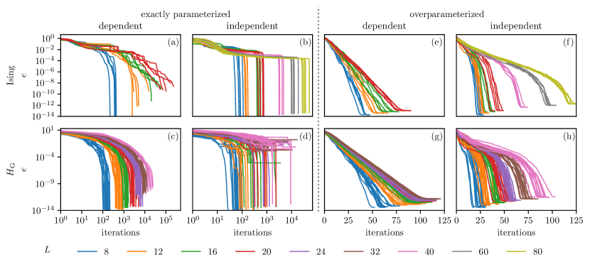
Figure 2: Cost function optimization traces exposing the differences between the minimizations as the protocol and target Hamiltonian change. The effect of circuit depth is probed using the exactly parameterized regime ($p=L/2$) and the overparameterized regime ($p=L^{2}/4$). The target Hamiltonian is (Top row): the Ising model, defined in Eq. (17), as the target Hamiltonian, and $5$ random initializations per value of $p$, lattice size and protocol. (Bottom row): $3$ randomly generated symmetric quadratic Hamiltonians, defined in Eq. (18), and $5$ random initializations per generated Hamiltonian, value of $p$, lattice size and protocol. When preparing the ground state of the Ising model (a), the site dependent protocol displays a "staircase" pattern, where the cost function undergoes little variation before dropping to a new plateau; in stark contrast, when preparing a generic symmetric FGS (c), it exhibits a smoother decrease. The site independent protocol presents the opposite behavior: when preparing the ground state of the Ising model (b), the cost initially undergoes a slow, but smooth, decrease, before sharply dropping when the state is prepared; when the target state is a generic symmetric FGS (d), the staircase pattern is again visible, this time also accompanied by local minima. This behavior is highlighted in Figure 9 in Appendix C. After increasing the depth of the circuit into the overparameterized regime, the differences in optimization between states vanish, and the cost function decrease becomes exponential with no local minima present.

Figure 2 shows the optimization traces after classically optimizing the algorithm. We compare two circuit depths: $p=L/2$ [41, 62, 100], which we have determined to be the minimum depth for which the protocol reaches maximum expressibility, and $p=L^{2}/4$, well into the overparameterized regime (as we quantify in Section 3.3), where the redundancy in parameters is known to greatly reduce the computational cost of the optimization [49, 50, 53, 54]. We defer a discussion of the latter for Section 3.3.

We observe that changing the target state and the protocol employed can drastically alter the characteristics of the optimization. In particular, we identify a “staircase" pattern, signaling a harder optimization problem, which is discernible at higher system sizes. It emerges both when employing the site dependent protocol to target the Ising model [Figure 2(a)], and when using the site independent protocol to target generic quadratic Hamiltonians [Figure 2(d)]. We discuss and propose a mechanism for this phenomenon in Appendix C, where we see that the cost function is not able to distinguish the target state from other states in the Hilbert space, even if they are orthogonal. It was argued in [4] that this behavior is not possible when the barren plateau phenomenon is present; here, we see that it can represent an intermediate behavior of the landscape as the size of the system increases and gradients begin to vanish (we study the scaling of the gradients in Appendix A). The efficient classical simulation of FGS is pivotal in observing it, as it is not as evident in smaller system sizes.

The only case susceptible to local minima is the site independent one at $p=L/2$ when targeting generic symmetric quadratic Hamiltonians [Figure 2(d)]. There, the optimization is highly sensitive to the initial condition, and the number of iterations to converge, along with the value found at the minimum, can vary drastically. This starkly contrasts with the other cases in Figure 2 — in particular, the one where we target the Ising model using the same protocol [Figure 2(b)]. While the average number of iterations to convergence is approximately the same in both cases, the former has a high standard deviation, as can be seen in Figure 5. Thus, using a protocol with less symmetry produces more consistent results which are not susceptible to local minima. This shows that imposing more symmetries may not always be desirable, as it may have an unpredictable effect in the optimization landscape and can result in local minima.

We now study how different properties of the target Hamiltonian can give rise to the phenomenology we previously observed and thereby explain Figure 2. One obvious property that distinguishes the Ising Hamiltonian, Eq. (17), from that of the random Hamiltonian in Eq. (18) is the presence of locality in the former case. Locality of the target Hamiltonian is known to influence whether the optimization associated to a quantum circuit will feature barren plateaus, with non-local terms presenting exponentially vanishing gradients [15]. Locality can also have an influence below system sizes at which barren plateaus appear, and it has been argued that long-range interactions in the target Hamiltonian make the optimization harder [89], resulting in higher values of the cost function at the optimum and requiring more iterations to converge. In our case, we will see that the influence of the locality of the target Hamiltonian on optimization depends on the constraints of the protocol being used. In particular, we will show that the site-independent and the site-dependent protocol behave differently in this respect, which explains the observed differences in the optimization.

We use three families of models to quantify how the locality of the target Hamiltonian affects the hardness of the optimization:

1. A special type of a long-range Ising Hamiltonian:

   $$H(\alpha) =-\sum_{r}e^{-\alpha r}\sum_{j}X_{j}Z_{j+1}Z_{j+2}\ldots Z_{j+r}X_{j+r+1}$$

   $$-\sum_{j}Z_{j},$$ (20)

   where $\alpha$ describes exponentially decaying interactions in a lattice. The choice of this Hamiltonian is motivated by the fact that its ground state can be expressed in terms of free fermions for any $\alpha$, unlike the related models with power-law decaying interactions recently studied in Refs. [42, 89].

2. $(k+2)$-local, symmetric, quadratic Hamiltonians

   $$H_{\text{LG}}(k) =i\sum_{jl}\tilde{h}_{jl}\gamma_{j}\gamma_{l},$$ (21)

   $$\tilde{h}_{jl} =\begin{cases}\mathrm{random},\;\mathrm{if}\;|j-l|<2(k+2),\\ 0,\;\mathrm{if}\;|j-l|\geq 2(k+2),\end{cases}$$

   which are derived from the randomly-generated generic symmetric quadratic Hamiltonians in Eq. (18) by setting $h_{jl}=0$ for any pair of Majoranas at a distance $\geq 2(k+2)$.

3. A cluster Ising model at criticality [21, 70]

   $$H_{\text{C}}(k) =-\sum_{j}X_{j}Z_{j+1}Z_{j+2}\ldots Z_{j+r}X_{j+k+1}$$

   $$-\sum_{j}Z_{j},$$ (22)

   for which the ground state in one of the gapped phases is a symmetry-protected topological state [78].

In the two latter models, interactions are strictly limited to sites at most $k+2$ sites away, while in the first model they are exponentially suppressed.

Figure 3 compares the effect of locality on the optimization. We vary the parameters controlling localization of the couplings in each of the models Eqs. (20)-(3), and we measure the success probability in the site-independent case or the number of iterations to converge in the site-dependent case. The success probability is defined as the ratio between the number of random initializations that resulted in the cost function dropping below numerical precision (and thus the target state being successfully prepared) versus the total number of initializations. This measure was not used as a benchmark for the site-dependent protocol, as this protocol is not susceptible to getting trapped in local minima, thus the success probability is always equal to one regardless of the locality of the Hamiltonian.

We see in Figure 3 that the more non-local the target Hamiltonian is, the lower the success probability is in the site-independent protocol. Surprisingly, however, we see that the more non-local the target Hamiltonian is, the lower the number of iterations is to converge is the site-dependent case. Both statements are verified for all the models introduced above. Thus, while locality makes it easier to prepare the target state using site-independent protocol, it makes the site-dependent protocol harder to optimize. We conclude that, on the one hand, the symmetry constraints in the site-independent protocol cause non-locality in the cost function to drive the optimization into difficult regions that trap it in local minima. The site-dependent case, on the other hand, is free to explore the entire manifold of FGS and bypass these traps, and non-local terms lead the optimization to converge faster, consistent with Figure 1(a), (b), (c).

Figure 3: Plots characterizing the effect of Hamiltonian locality on optimization hardness in both the site-dependent and site-independent protocols in the exactly parameterized regime using PBCs. Horizontal axes are the parameters $k$ and $\alpha$, which control the locality of the Hamiltonians studied. On the left, the $y$- axis shows the success ratio, defined as the ratio between the number of random initializations which ended in state preparation and all random initializations. In the right panel, the $y$-axis is the (logarithm of) total number of iterations to converge. The labels refer to the target Hamiltonians defined in Eqs. (20), (21) and (3). Lattice sizes used were either $12$ or $16$. Between 20 and 150 random initialisations were computed for each Hamiltonian parameter in the site dependent cases, and between 200 and 500 were computed in the site independent ones; solid line is the mean value, while the shaded area indicates standard deviation.

3.3 Overparameterized regime

It has been pointed out [103, 49] that taking the circuit depth to be very large, the optimization associated with Eq. (1) becomes considerably easier – a phenomenon dubbed overparameterizaton. The onset of the overparameterized regime has been argued to correspond the circuit depth at which the Quantum Fisher Information Metric saturates at every point $\theta$ in the optimization landscape [54, 37]. This is equivalent to the circuit depth at which an increase in $p$ does not lead to an increase in the states that can be prepared by the variational circuit Eq. (2), i.e., the circuit depth corresponding to $\hat{p}$ as defined in Section 2.2. We numerically confirm this to be the case for all the cases discussed at the end of Section 3.1.

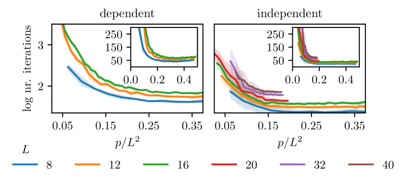
Figure 4: Number of iterations to converge vs. the circuit depth in the overparameterized regime. We see a decrease, consistent between different system sizes, when employing a circuit depth proportional to $L^{2}$. This reduction in the number of iterations is at first pronounced but then tapers off until it finally saturates. The insets use a linear scale for the vertical axis; they emphasize the point at which this saturation is reached. The target Hamiltonian is that of the Ising model, Eq. (17). Between 5 and 40 random initilisations were performed for each circuit depth; solid lines represent the mean value, and the shaded area indicates standard deviation.

.

We perform a scaling analysis of the number of iterations that the optimizer takes to prepare the state as the depth of the circuit increases well into the overparameterized regime. We find that, as depth increases, the average number of iterations to converge initially suffers a large initial decay, until it slows down and saturates at $p\sim L^{2}$, i.e., no further increase in circuit depth provides a decrease in the average number of iterations to converge. We observe this trend consistently between different optimizers and different system sizes, the latter shown in Figure 4, where an exponential decay is seen. Further, by comparing how the average number of iterations the optimizer takes to converge scales with lattice size, both when the circuit depth is equal to $\hat{p}$ and into the overparameterized regime, we see that what is initially a polynomial scaling turns into a linear scaling with lattice size – see Figure 5.

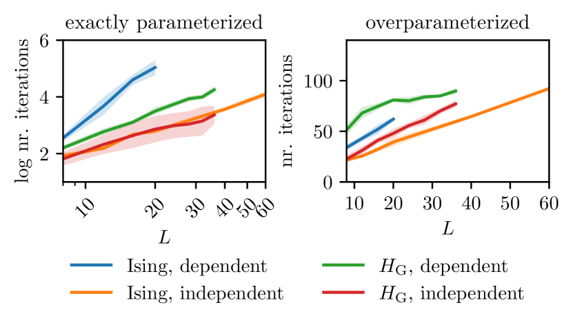
Figure 5: Number of iterations to converge vs. lattice size corresponding to the data in Figure 2. Solid line is the mean value, the shaded area indicates the standard deviation. The legend refers to the Hamiltonian targetted and protocol used, in this order. The target Hamiltonians are either the Ising model, Eq. (17), or generic symmetric quadratic Hamiltonians, Eq. (18). The number of iterations to converge scales polynomially with system size when $p=L/2$ (left), which is the minimum circuit depth for maximum expressibility. This turns into a linear scaling as the circuit enters the overparameterized regime (right).

From the above, we note that the overparameterized regime effectively represents a shift in the workload from the quantum computer to the classical one and vice-versa, as increasing the number of parameters makes the classical optimization easier, but the preparation of the state in the quantum computer harder given the increased circuit depth (and corresponding time to run the circuit, see Appendix D). Thus, as noise levels in a device decrease, increasing the depth of the circuit allows variational algorithms to take immediate advantage of these advancements. This has the caveat that when the number of parameters passes a certain threshold, the overhead associated with certain algorithms, such as BFGS, exceeds the advantage obtained from overparameterizing the circuit; we quantify this in Appendix D. In this case, algorithms designed to handle a large number of parameters, such as ADAM or stochastic gradient descent, should be employed instead.

Since in the site dependent case each circuit layer has $\sim L$ parameters, the behavior we have just described in terms of circuit depth $p\sim L^{2}$ corresponds to $\sim L^{3}$ parameters in this case. As all quantities in Table 1 scale quadratically or linearly with system size, the phenomenon of overparameterisation can neither be explained by the saturation of the manifold of preparable states nor by the saturation of the manifold of unitaries. In what follows, we propose and test an explanation for gradient based optimizers in terms of a change in the very properties of the parameterisation of the manifold as the circuit depth increases.

A gradient based optimizer is an algorithm that, given an initial condition $\theta_{0}$, iterates the following update function

$$\theta_{i+1}=\theta_{i}-\eta A\nabla e(\theta_{i})$$

until it converges, that is, it can not find a value of $\eta$, called the learning rate, such that the update reduces the cost function $e$. The matrix $A$ is a bias that provides extra information to the algorithm. It can be the inverse of the Hessian $H^{-1}$ in the case of Newton based methods (or an approximation of it as in the case of quasi-Newton methods such as BFGS), or the inverse of the metric of the manifold being optimized over, as is is done in e.g. Quantum Natural Gradient descent methods [85]. Importantly, the gradient of a function is a linear local approximation of the function at that point. While that means that, if $\mathinner{\!\left\lVert\nabla e\right\rVert}\neq 0$, there is a value of $\eta$ such that $e(\theta_{i+1})<e(\theta)$, it does not offer any real guarantee about the actual change $\Delta e_{i+1}=e(\theta_{i})-e(\theta_{i+1})$.

Here, we examine how good this local approximation is as the optimization progresses, both when the circuit depth is equal to $\hat{p}$ and in the overparameterized regime. We run the BFGS algorithm, and the learning rate is picked on a per-iteration basis by using the strong Wolfe conditions, an established heuristic based on a minimum descent criterion [69]. This is a quasi-Newton method, and so $A=\widetilde{H^{-1}}$ will be an approximation to the inverse of the Hessian. In Figure 6, we plot

$$l=\frac{\Delta e_{i}}{||\widetilde{H^{-1}}\nabla e_{i}||_{2}\Delta\theta_{i}},$$ (23)

which quantifies how much of the variation in the cost function can be attributed to the local approximation given by the gradient at the $i$th iteration. We see that in the overparameterized regime, most of the variation in the cost is accounted for by this approximation, and that it concentrates around an average of $\tilde{k}$ leading to the exponential decay seen in Figure 2 following the equation ${\partial e}/{\partial\theta}=\tilde{k}e$. We conclude that the overparameterized regime leads to parameterizations that are more amenable to optimization, as they capture the variation in the cost for longer distances in the parameter space (see panel 3 in Figure 1).

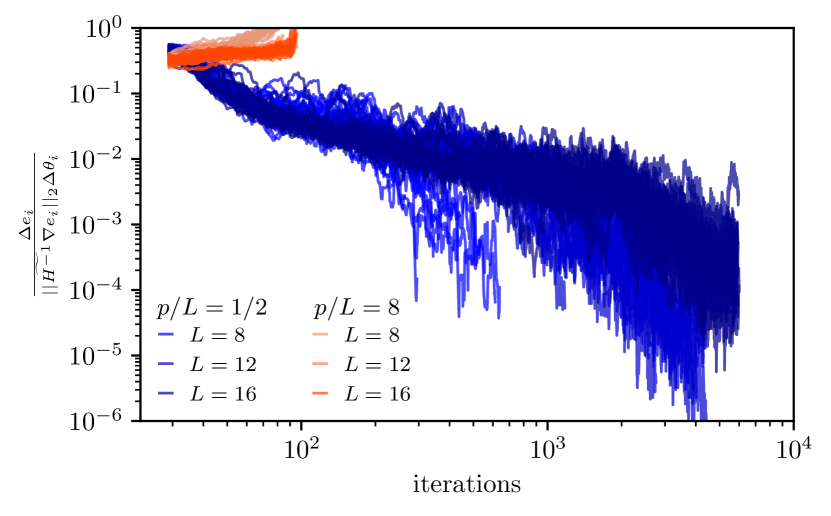
Figure 6: Quantification of how well the gradient accounts for the change in the cost function along the optimization, both in the exactly parameterized ($p=L/2$) and in the overparameterized ($p/L=8$) regimes. The plot shows the quantity defined in Eq. (23) recorded throughout the optimization. We see that in the overparameterized regime, the value of the gradient consistently predicts the decrease in the cost function up to a constant factor; while it only accounts for a decreasing fraction of this variation in the exactly parameterized regime. Here, the target state was that of the Ising model with PBCs.

4 Conclusion

By deriving the corresponding Lie algebra structure, we showed that the original QAOA protocol on a 1D lattice can prepare all fermionic Gaussian states satisfying the symmetries of the circuit, and we have numerically determined the circuit depth needed to achieve maximum expressibility. The efficient classical simulation of these states was employed to systematically study the optimization associated to these protocols.

We observed that decoupling the angles of the protocol makes the preparation of non-local states easier, and of local states harder, which is the opposite of what is observed when the angles are coupled. We argued that this is due to the symmetries in the system constraining the features available to the optimizer. Further, we studied in detail the overparameterized regime, exploiting the larger system sizes and circuit depths accessible to us, where we find that the number of iterations to converge to the solution scales linearly with system size. Moreover, we found that the number of iterations to converge to the solution decreases exponentially with the depth of the circuit, until it saturates at a depth which is quadratic in system size. Finally, we observed that the improvement in the optimization can be explained in terms of of better local linear approximations provided by the gradients.

Beyond elucidating the current knowledge on the interplay between symmetry and optimization, and furthering the understing on the overparameterized regime of optimization, our work can serve as the basis for a benchmarking scheme for the implementation of variational algorithms in quantum computers. These have already been performed using free states such as, e.g., Majorana zero modes [87] or the ground state of the Ising model [16]; this scheme could potentially be leveraged into error correcting methods [12]. Moreover, it provides a framework to better understand the theory behind the preparation of free states using variational algorithms, already studied in models such as the Ising model [41, 22], the Kitaev model in the exactly solvable limit [45], or the cluster model [70]. Furthermore, while there are established algorithms to build circuits that prepare FGS [47, 51], these require a full description of the corresponding covariance matrix; a variational approach is relevant where this structure is not known beforehand e.g. when approximating interacting states [70, 61] or maximizing a quantity of interest such as magic [39, 72]. Finally, by fully characterizing these circuits on 1D lattices, we open the possibility to describe more complex graphs in terms of simpler ones following a divide-and-conquer strategy [30, 111].

5 Acknowledgements

This work was supported by the Leverhulme Trust Research Leadership Award RL-2019-015, by EPSRC grant EP/R020612/1 and by the German Federal Ministry of Education and Research (BMBF) through the funded project EQUAHUMO (Grant No. 13N16066) within the funding program quantum technologies - from basic research to market, in association to the Munich Quantum Valley. CNS acknowledges financial support from the UK Hub in Quantum Computing and Simulation, part of the UK National Quantum Technologies Programme with funding from UKRI EPSRC grant EP/T001062/1. KM acknowledges financial support from the Royal Commission for the Exhibition of 1851. Statement of compliance with EPSRC policy framework on research data: This publication is theoretical work that does not require supporting research data.

Appendix A Variance of gradient

Here, we study how the variance of the gradient with respect to the center angle scales with the lattice size and the circuit depth. This variance is known to capture the phenomenon of barren plateaus, as it provides an upper bound for the magnitude of the gradients across the optimization landscape [63, 43]. The scaling with respect to the center angle is taken to be representative of the scaling with respect to the other angles [4].

Figure 7 illustrates the scaling of this variance with the lattice size, expressed in terms of the dimension of the Lie algebra, following Ref. [53] which conjectured that the variance of the gradient is inversely proportional to this dimension. We see that while this seems to hold in general, it depends on the circuit depth and the state under peparation. When preparing the Ising model, increasing the circuit depth changes this proportionality by a constant factor; while, curiously, when preparing generic FGS with the site dependent protocol, it is independent of the circuit depth. Note also that when the circuit enters the overparameterized regime, for instance when targeting the Ising model in the site-independent case at $p=7L$, this relation can break down as the variance of the gradient saturates at high circuit depths (see next paragraph). Finally, we note that there are exceptions to this relation; in particular, we note that when preparing a generic FGS using the site independent protocol, the gradient seems to oscillate around a constant value of $\sim 10$ without decaying as the system size increases.

Figure 8 illustrates the scaling of the variance of the gradient with circuit depth. We see that when targeting the Ising model, there is an initial drop in this variance, which then stabilizes to a fixed value. In contrast, when preparing a generic FGS, the variance almost immediately converges to this stable value, particularly in the site-dependent case.

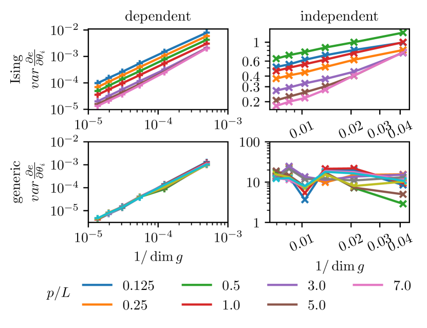
Figure 7: Variance of gradient taken at center angle $||\partial e/\partial\theta_{i}||$ using the site-dependent protocol (left) and the site-independent protocol (right) with the ground state of the Ising model as a target state (top) and $5$ generic quadratic Hamiltonians (symmetric quadratic Hamiltonians in the independent case) as a target state (bottom), plotted against the inverse of the dimension of the Lie algebra generated by the Hamiltonians used in each protocol at different system sizes. Various values of $p/L$ (bottom labels) between $1$ and $7$ were used. 20000 samples were taken per value of $p$, random state and lattice size.

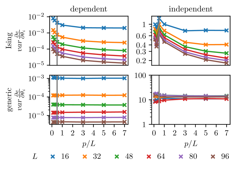
Figure 8: Variance of gradient taken at center angle $||{\partial e}/{\partial\theta_{i}}||$ using the site-dependent protocol (left) and the site-independent protocol (right) with the ground state of the Ising model as a target state (top) and $5$ generic quadratic Hamiltonians (symmetryc generic quadratic Hamiltonians in the independent case) as a target state (bottom), plotted against various values of $p$ between $1$ and $4L$. Several system sizes (bottom labels) were used. 20000 samples were taken per value of $p$, random state and lattice size. The vertical line indicates $p=L/2$.

Appendix B Lie algebra structure

Here, we deduce the structure of the Lie algebras associated with the protocols in Eqs. (1)-(2) for both OBCs and PBCs. We do so by deriving a basis for the algebras generated by the aforementioned sets when unrestricted to any symmetry sector. Then, we restrict these bases to a fixed parity symmetry sector, and see how this affects the structure and dimensions of the algebra. Note that, for notational simplicity, throughout this section we often disregard signs when converting from spin to Majorana operators when it does not influence the generated Lie algebras.

Let us recall the fermionic parity operator

$$P=\prod_{j}Z_{j}.$$

Lemma 1.

The Lie algebra generated by $\mathcal{D}=\{iZ_{j},iX_{j}X_{j+1}\}_{j=1,...L}$

1. with OBC is

   $$\mathfrak{d}_{\text{OBC}}=\{iZ_{j}, iX_{j}Z...ZX_{k},X_{j}Z...ZY_{k},$$ (24)

   $$iY_{j}Z...ZX_{k},Y_{j}Z...ZY_{k}\mathrel{\mathop{\mathchar 58\relax}}$$

   $$1\leq j<k\leq L\}$$

   $$=\{\gamma_{j}\gamma_{k} \mathrel{\mathop{\mathchar 58\relax}}1\leq j<k\leq L\}$$ (25)

   and has dimension $L(2L-1)$.

2. with PBC is

   $$\mathfrak{d}_{\text{PBC}} =\mathfrak{d}_{\text{OBC}}\cup(P\cdot\mathfrak{d}_{\text{OBC}})$$ (26)

   where

   $$(P\cdot\mathfrak{d}_{\text{OBC}})=\{ iZ...Z_{j-1}Z_{j+1}...Z,\quad iZ...ZX_{j}X_{k}Z...Z,$$

   $$iZ...ZX_{j}Y_{k}Z...Z,\quad Z...ZY_{j}X_{k}Z...Z,$$

   $$iZ...ZY_{j}Y_{k}Z...Z\quad\mathrel{\mathop{\mathchar 58\relax}}1\leq j<k\leq L\}$$ (27)

   and this algebra has dimension $2L(2L-1)$.

Lemma 2.

The Lie algebra generated by $\mathcal{I}=\{i\sum_{j}Z_{j},i\sum_{j}X_{j}X_{j+1}\}$

1. with OBC is

   $$\mathfrak{i}_{\text{OBC}}=\{ iZ_{j}+iZ_{L-j+1},$$ (28)

   $$iX_{j}Z...ZX_{k}+iX_{L-k+1}Z...ZX_{L-j+1},$$

   $$iX_{j}Z...ZY_{k}+iY_{L-k+1}Z...ZX_{L-j+1},$$

   $$iY_{j}Z...ZX_{k}+iX_{L-k+1}Z...ZY_{L-j+1},$$

   $$iY_{j}Z...ZY_{k}+iY_{L-k+1}Z...ZY_{L-j+1},$$

   $$1\leq j<k\leq\lceil L/2\rceil\}$$

   $$=\{ \gamma_{2j-1}\gamma_{2j}+\gamma_{2L-2j+1}\gamma_{2L-2j+2},$$ (29)

   $$\gamma_{2j}\gamma_{2k-1}+\gamma_{2L-2k+2}\gamma_{2L-2j+1},$$

   $$\gamma_{2j}\gamma_{2k}-\gamma_{2L-2k+2}\gamma_{2L-2j+2},$$

   $$\gamma_{2j-1}\gamma_{2k-1}-\gamma_{2L-2k+1}\gamma_{2L-2j+1},$$

   $$\gamma_{2j-1}\gamma_{2k}+\gamma_{2L-2k+1}\gamma_{2L-2j+2},$$

   $$\mathrel{\mathop{\mathchar 58\relax}}1\leq j<k\leq\lceil L/2\rceil\},$$

   and this algebra has dimension $L^{2}$ [53].

2. with PBC is

   $$\mathfrak{i}_{\text{PBC}}=\{ i\sum_{j}(Z_{j}+Z_{1}...Z_{j-1}Z_{j+1}...Z_{L}),$$ (30)

   $$i\sum_{j}(X_{j}Z...ZX_{j+k}$$

   $$+Z_{1}...Z_{j-1}X_{j}X_{j+(L-k)}Z_{j+(L-k)+1}...Z_{L}),$$

   $$i\sum_{j}(X_{j}Z...ZY_{j+k}+Y_{j}Z...ZX_{j+k}$$

   $$+Z_{1}...Z_{j-1}X_{j}Y_{j+(L-k)}Z_{j+(L-k)+1}...Z_{L}$$

   $$+Z_{1}...Z_{j-1}Y_{j}X_{j+(L-k)}Z_{j+(L-k)+1}...Z_{L}),$$

   $$i\sum_{j}(Y_{j}Z...ZY_{j+k}$$

   $$+Z_{1}...Z_{j-1}Y_{j}Y_{j+(L-k)}Z_{j+(L-k)+1}...Z_{L})$$

   $$\mathrel{\mathop{\mathchar 58\relax}}1\leq k\leq L-1\}$$

and has dimension $3L-2$.

The proofs for these statements follow by inductively taking the brackets of the generators of these algebras. Here, we provide a proof for the structure of $\mathfrak{d}_{\text{OBC}}$; the others are derived in a similar fashion.

Proof.

By induction on $L$:

$L=2$: Taking the Lie brackets iteratively of $\{iZ_{1},Z_{2},iX_{1}X_{2}\}$, one obtains the linearly independent set $\{iZ_{1},iZ_{2},iX_{1}X_{2},iX_{1}Y_{2},iY_{1}X_{2},iY_{1}Y_{2}\}$, which has $6$ elements.

$L\implies L+1$: Assume the Lemma holds for $L$. Then, define

$$\mathcal{G}_{a,b}\mathrel{\mathop{\mathchar 58\relax}}=\{iZ_{j},iX_{j}X_{j+1}\}_{j=a,...,b}$$ (31)

$$\mathcal{L}_{a,b}\mathrel{\mathop{\mathchar 58\relax}}=\{ iZ_{j},iT_{j,k}\mathrel{\mathop{\mathchar 58\relax}}a\leq j<k\leq b\}$$ (32)

$$T_{j,k}\mathrel{\mathop{\mathchar 58\relax}}= A_{j}\otimes\left(\bigotimes_{m=j+1}^{k-1}Z_{m}\right)\otimes B_{k},$$

$$A_{m},B_{m}\in\{X_{m},Y_{m}\}$$ (33)

and let $\mathcal{R}_{a,b}$ be the Lie algebra generated by $\mathcal{G}_{a,b}$. We must prove that $\mathcal{R}_{1,L+1}=\mathcal{L}_{1,L+1}$.

By induction hypothesis $\mathcal{R}_{1,L}=\mathcal{L}_{1,L}$. Using this, and the definition of Lie algebra generators, we obtain $\mathcal{L}_{1,L}\subseteq\mathcal{R}_{1,L+1}$. Since it is easy to prove that

$$\left[iT_{i,j},iT_{k,l}\right]\propto\delta_{jk}iT_{i,l},$$ (34)

and $\left[iT_{i,j},iZ_{k}\right]\propto(\delta_{ik}+\delta_{jk})iT_{i,j}$, we conclude that $\mathcal{R}_{1,L+1}\setminus\mathcal{L}_{1,L}\subseteq\{iT_{k,L+1}\}_{k=1,...,L}\cup\{iZ_{L+1}\}$. But $T_{k,L+1}\subset\mathcal{L}_{k,L+1}=\mathcal{R}_{k,L+1}\subseteq\mathcal{R}_{1,L+1}$, and $Z_{L+1}\in\mathcal{G}_{1,L+1}$. Thus it must be the case that $\mathcal{R}_{1,L+1}=\mathcal{L}_{1,L+1}$.

Since, from the above, $\mathcal{L}_{1,L+1}=\mathcal{L}_{1,L}\cup\{T_{k,L+1}\}_{k=1,...,L}\cup\{Z_{L+1}\}$, and since these sets are disjoint, using the induction hypothesis, the dimension of $\mathcal{L}_{1,L+1}$ is $L(2L-1)+4L+1=(L+1)(2(L+1)-1)$ ∎

Noting that every element of the generators of the Lie algebras commute with $P$, we now state the structure of these algebras restricted to each of the parity symmetry sectors.

We first note that, as can be seen in Lemma 1 for the generators $\mathcal{D}$, when restricting to a parity sector, the algebra in the OBC case remains unchanged, while the algebra in the PBC case is cut in half, and is equal to former. Hence:

$$\mathfrak{d}\mathrel{\mathop{\mathchar 58\relax}}= \,\mathfrak{d}_{\text{OBC}}=\mathfrak{d}_{\text{OBC}}\Big{|}_{P=\pm 1}=\mathfrak{d}_{\text{PBC}}\Big{|}_{P=\pm 1}$$ (35)

and it has dimension $L(2L-1)$.

As for the case of the set of generators $\mathcal{I}$, we see that the algebra with OBC remains unchanged when restricted to a parity sector. Hence

$$\mathfrak{i}_{\text{OBC}}=\mathfrak{i}_{\text{OBC}}\Big{|}_{P=\pm 1}$$ (36)

and it has dimension $L^{2}$.

Finally, the same set of generators with PBC yields

$$\mathfrak{i}_{\text{PBC}}\Big{|}_{P=\pm 1}=\Bigl{\{} i\sum_{j}Z_{j},$$ (37)

$$i\sum_{j}(X_{j}Z...ZX_{j+k}\mp Y_{j}Z...ZY_{j+N-k}),$$

$$i\sum_{j}(X_{j}Z...ZY_{j+k}+Y_{j}Z...ZX_{j+k}$$

$$\pm X_{j}Z...ZY_{j+N-k}\pm Y_{j}Z...ZX_{j+N-k}),$$

$$i\sum_{j}(Y_{j}Z...ZY_{j+k}\mp X_{j}Z...ZX_{j+N-k})\mathrel{\mathop{\mathchar 58\relax}}$$

$$1\leq k\leq L-1\Bigr{\}}$$

$$=\Bigl{\{} \sum_{j}\gamma_{2j-1}\gamma_{2j},$$

$$\sum_{j}\gamma_{2j}\gamma_{2(j+k)-1}\pm\gamma_{2j-1}\gamma_{2(j+N-k)},$$

$$\sum_{j}\gamma_{2j}\gamma_{2(j+k)}-\gamma_{2j}\gamma_{2(j+k)-1}$$

$$\pm\gamma_{2j}\gamma_{2(j+N-k)-1}\mp\gamma_{2j-1}\gamma_{2(j+N-k)-1},$$

$$\sum_{i}\gamma_{2j-1}\gamma_{2(j+k)}\pm\gamma_{2j}\gamma_{2(j+N-k)-1}$$

$$\mathrel{\mathop{\mathchar 58\relax}}1\leq k\leq L-1\Bigr{\}}$$ (38)

and it has dimension $\lfloor 3L/2\rfloor$.

Appendix C Mechanism behind staircases

In Section 3.2, we described a pattern that we dubbed "staircase", where the optimizer gets stuck and the value of the cost function undergoes very little variation for a number of iterations until it sharply drops to a new plateau; we highlight this phenomenon more clearly in Figure 9. Here, we offer an explanation for this observation.

In Figure 10, we plot the overlap of the state along the optimization with the eigenstates of the target Hamiltonian. We notice that the overlap of the state under preparation with the target Hamiltonian is orders of magnitude higher than with other excited eigenstates. The dynamics of state preparation is thus dominated by a competition between the ground state and the first excited state. We propose that the staircase plateaus we observe follow a similar mechanism: in each plateau, there is a state in the Hilbert space (akin to the first excited state in the previous description) that fully captures the features that the cost function struggles to distinguish from those of the ground state in each of these plateaus.

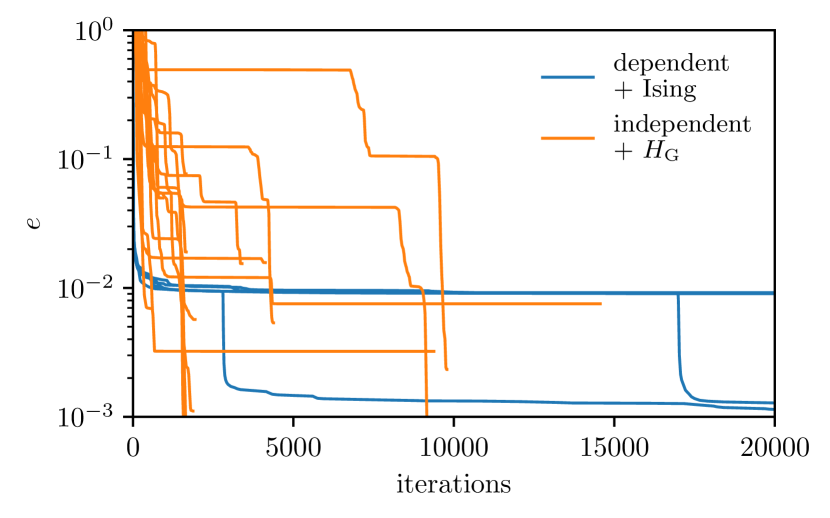
Figure 9: Optimization traces showing the “staircase" pattern previously seen in Figure 2. Here, the system size is $40$, and the label refers to the protocol used and the Hamiltonian targetted, respectively. The target Hamiltonian is either the Ising model, Eq. (17), or a generic symmetric quadratic Hamiltonian, Eq. (18)). PBCs and exact parameterization ($p=L/2$) are assumed.

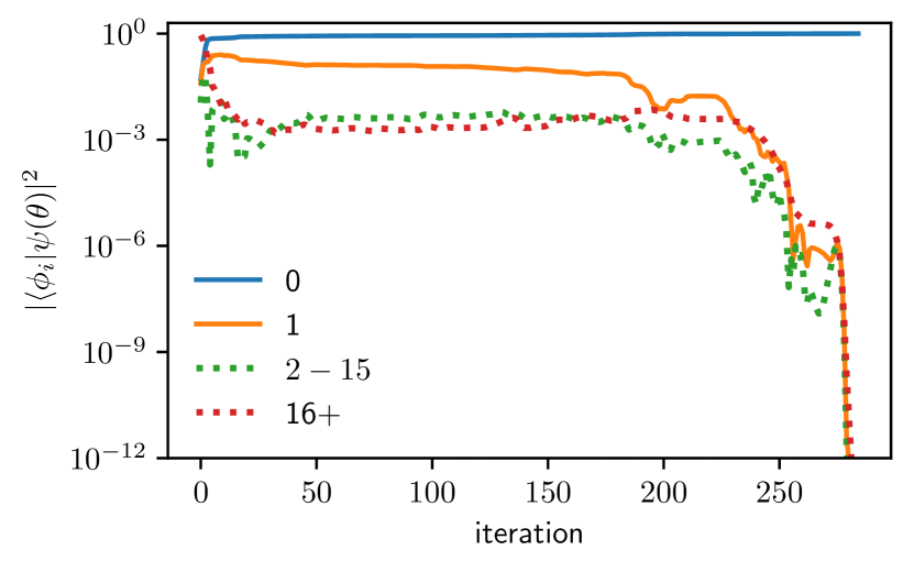
Figure 10: Overlaps of lowest excited states of the target Hamiltonian with the state under preparation $\ket{\psi(\theta_{i})}$. Legend indicates the index of an eigenstate with which overlaps were taken, with $0$ indicating the ground state, $1$ indicating the first excited state, etc., while the ranges indicate a sum of the overlaps with the corresponding eigenstates. We see a high overlap with the first excited state throughout the optimization, indicating that the cost function cannot easily distinguish this state from the ground state. The site-independent protocol was used and the Ising model (17) was targeted at the exactly parameterized depth $p=L/2$ for $L=16$.

Appendix D Scaling of Hessian and optimization

In Figure 11, we examine the effect of increasing the circuit depth on the total time taken to run an optimization and on the time it would take to prepare these states on a quantum simulator (measured by the sum of the angles). We see that despite increasing the circuit depth into the overparameterized regime making the optimization easier, the sum of the angles in the protocol grows linearly with the circuit depth, increasing the time to run the circuit on a quantum simulator and making it more prone to errors. Furthermore, we see that despite the number of iterations to converge decreasing into the overparameterized regime, when one looks at the actual time taken to run the optimizer, there is an inflexion point where it first goes down and then starts increasing again. This is due to the algorithm (BFGS) used, which stores an approximation to the Hessian; as the size of the Hessian increases, the computational cost associated to storing and manipulating it dominates the computational time. Thus, while it is feasible to a larger class of optimization algorithms at lower system sizes, as one increases the circuit depth, one has to switch to algorithms specialized to dealing with a large number of parameters e.g. ADAM or stochastic gradient descent.

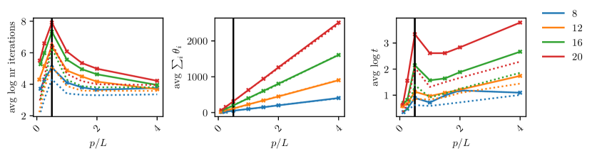
Figure 11: Different quantities characterizing the hardness of the optimization with increasing circuit depth. On the left, we plot the mean of the logarithm of the number iterations to converge; the center plot depicts the mean of the sum of all the angles of the protocol, where periodicity is appropriately taken into account; on the right, the average of the logarithm of the total computational time is shown. Generic symmetric quadratic Hamiltonians were targeted, and results were averaged over 5 random states and 5 random initializations per state. Filled line corresponds to the site-dependent protocol, while dotted line represents the site-independent protocol; these two cases essentially display the same behavior. Periodic boundary conditions were used, and the black vertical line indicates $p=L/2$, the depth at which the circuit is exactly parameterized. These results were obtained on an Intel(R) Xeon(R) CPU E5-2650 v4 @ 2.20GHz.

References

- Abbas et al. [2021] Amira Abbas, David Sutter, Christa Zoufal, Aurelien Lucchi, Alessio Figalli, and Stefan Woerner. The power of quantum neural networks. Nature Computational Science, 1(6):403–409, 2021. ISSN 2662-8457. doi: 10.1038/s43588-021-00084-1. URL https://doi.org/10.1038/s43588-021-00084-1.
- Akshay et al. [2022] V. Akshay, H. Philathong, E. Campos, D. Rabinovich, I. Zacharov, Xiao-Ming Zhang, and J. Biamonte. On circuit depth scaling for quantum approximate optimization, 2022. URL https://arxiv.org/abs/2205.01698.
- Albertini and D’Alessandro [2001] F. Albertini and D. D’Alessandro. Notions of controllability for quantum mechanical systems, 2001. URL https://arxiv.org/abs/quant-ph/0106128.
- Arrasmith et al. [2021] Andrew Arrasmith, Zoë Holmes, M. Cerezo, and Patrick J. Coles. Equivalence of quantum barren plateaus to cost concentration and narrow gorges, 2021. URL https://arxiv.org/abs/2104.05868.
- Arute et al. [2020] Frank Arute, Kunal Arya, Ryan Babbush, Dave Bacon, Joseph C. Bardin, Rami Barends, Sergio Boixo, Michael Broughton, Bob B. Buckley, David A. Buell, Brian Burkett, Nicholas Bushnell, Yu Chen, Zijun Chen, Benjamin Chiaro, Roberto Collins, William Courtney, Sean Demura, Andrew Dunsworth, Edward Farhi, Austin Fowler, Brooks Foxen, Craig Gidney, Marissa Giustina, Rob Graff, Steve Habegger, Matthew P. Harrigan, Alan Ho, Sabrina Hong, Trent Huang, William J. Huggins, Lev Ioffe, Sergei V. Isakov, Evan Jeffrey, Zhang Jiang, Cody Jones, Dvir Kafri, Kostyantyn Kechedzhi, Julian Kelly, Seon Kim, Paul V. Klimov, Alexander Korotkov, Fedor Kostritsa, David Landhuis, Pavel Laptev, Mike Lindmark, Erik Lucero, Orion Martin, John M. Martinis, Jarrod R. McClean, Matt McEwen, Anthony Megrant, Xiao Mi, Masoud Mohseni, Wojciech Mruczkiewicz, Josh Mutus, Ofer Naaman, Matthew Neeley, Charles Neill, Hartmut Neven, Murphy Yuezhen Niu, Thomas E. O’Brien, Eric Ostby, Andre Petukhov, Harald Putterman, Chris Quintana, Pedram Roushan, Nicholas C. Rubin, Daniel Sank, Kevin J. Satzinger, Vadim Smelyanskiy, Doug Strain, Kevin J. Sung, Marco Szalay, Tyler Y. Takeshita, Amit Vainsencher, Theodore White, Nathan Wiebe, Z. Jamie Yao, Ping Yeh, and Adam Zalcman. Hartree-fock on a superconducting qubit quantum computer. Science, 369(6507):1084–1089, 2020. doi: 10.1126/science.abb9811. URL https://www.science.org/doi/abs/10.1126/science.abb9811.
- Barron et al. [2021] George S. Barron, Bryan T. Gard, Orien J. Altman, Nicholas J. Mayhall, Edwin Barnes, and Sophia E. Economou. Preserving symmetries for variational quantum eigensolvers in the presence of noise. Phys. Rev. Applied, 16:034003, Sep 2021. doi: 10.1103/PhysRevApplied.16.034003. URL https://link.aps.org/doi/10.1103/PhysRevApplied.16.034003.
- Benedetti et al. [2019] Marcello Benedetti, Erika Lloyd, Stefan Sack, and Mattia Fiorentini. Parameterized quantum circuits as machine learning models. Quantum Science and Technology, 4(4):043001, nov 2019. doi: 10.1088/2058-9565/ab4eb5. URL https://doi.org/10.1088/2058-9565/ab4eb5.
- Biamonte [2021] Jacob Biamonte. Universal variational quantum computation. Phys. Rev. A, 103:L030401, Mar 2021. doi: 10.1103/PhysRevA.103.L030401. URL https://link.aps.org/doi/10.1103/PhysRevA.103.L030401.
- Bokhan et al. [2022] Denis Bokhan, Alena S. Mastiukova, Aleksey S. Boev, Dmitrii N. Trubnikov, and Aleksey K. Fedorov. Multiclass classification using quantum convolutional neural networks with hybrid quantum-classical learning, 2022. URL https://arxiv.org/abs/2203.15368.
- Boulebnane et al. [2022] Sami Boulebnane, Xavier Lucas, Agnes Meyder, Stanislaw Adaszewski, and Ashley Montanaro. Peptide conformational sampling using the quantum approximate optimization algorithm, 2022. URL https://arxiv.org/abs/2204.01821.
- Bravo-Prieto et al. [2019] Carlos Bravo-Prieto, Ryan LaRose, M. Cerezo, Yigit Subasi, Lukasz Cincio, and Patrick J. Coles. Variational quantum linear solver, 2019. URL https://arxiv.org/abs/1909.05820.
- Cade et al. [2020] Chris Cade, Lana Mineh, Ashley Montanaro, and Stasja Stanisic. Strategies for solving the fermi-hubbard model on near-term quantum computers. Phys. Rev. B, 102:235122, Dec 2020. doi: 10.1103/PhysRevB.102.235122. URL https://link.aps.org/doi/10.1103/PhysRevB.102.235122.
- Calabrese and Cardy [2004] Pasquale Calabrese and John Cardy. Entanglement entropy and quantum field theory. Journal of Statistical Mechanics: Theory and Experiment, 2004(06):P06002, jun 2004. doi: 10.1088/1742-5468/2004/06/p06002. URL https://doi.org/10.1088/1742-5468/2004/06/p06002.
- Cerezo et al. [2021a] M. Cerezo, Andrew Arrasmith, Ryan Babbush, Simon C. Benjamin, Suguru Endo, Keisuke Fujii, Jarrod R. McClean, Kosuke Mitarai, Xiao Yuan, Lukasz Cincio, and Patrick J. Coles. Variational quantum algorithms. Nature Reviews Physics, 3(9):625–644, 2021a. ISSN 2522-5820. doi: 10.1038/s42254-021-00348-9. URL https://doi.org/10.1038/s42254-021-00348-9.
- Cerezo et al. [2021b] M. Cerezo, Akira Sone, Tyler Volkoff, Lukasz Cincio, and Patrick J. Coles. Cost function dependent barren plateaus in shallow parametrized quantum circuits. Nature Communications, 12(1):1791, 2021b. ISSN 2041-1723. doi: 10.1038/s41467-021-21728-w. URL https://doi.org/10.1038/s41467-021-21728-w.
- Cervera-Lierta [2018] Alba Cervera-Lierta. Exact Ising model simulation on a quantum computer. Quantum, 2:114, December 2018. ISSN 2521-327X. doi: 10.22331/q-2018-12-21-114. URL https://doi.org/10.22331/q-2018-12-21-114.
- Chen et al. [2021] Ranyiliu Chen, Benchi Zhao, and Xin Wang. Variational quantum algorithm for schmidt decomposition, 2021. URL https://arxiv.org/abs/2109.10785.
- Cong et al. [2019] Iris Cong, Soonwon Choi, and Mikhail D. Lukin. Quantum convolutional neural networks. Nature Physics, 15(12):1273–1278, 2019. ISSN 1745-2481. doi: 10.1038/s41567-019-0648-8. URL https://doi.org/10.1038/s41567-019-0648-8.
- D’Alessandro [2007] D. D’Alessandro. Introduction to Quantum Control and Dynamics. Chapman & Hall/CRC Applied Mathematics & Nonlinear Science. CRC Press, 2007. ISBN 9781584888833. doi: https://doi.org/10.1201/9781584888833.
- Deller et al. [2022] Yannick Deller, Sebastian Schmitt, Maciej Lewenstein, Steve Lenk, Marika Federer, Fred Jendrzejewski, Philipp Hauke, and Valentin Kasper. Quantum approximate optimization algorithm for qudit systems with long-range interactions, 2022. URL https://arxiv.org/abs/2204.00340.
- Doherty and Bartlett [2009] Andrew C. Doherty and Stephen D. Bartlett. Identifying phases of quantum many-body systems that are universal for quantum computation. Phys. Rev. Lett., 103:020506, Jul 2009. doi: 10.1103/PhysRevLett.103.020506. URL https://link.aps.org/doi/10.1103/PhysRevLett.103.020506.
- Dreyer et al. [2021] Henrik Dreyer, Mircea Bejan, and Etienne Granet. Quantum computing critical exponents. Phys. Rev. A, 104:062614, Dec 2021. doi: 10.1103/PhysRevA.104.062614. URL https://link.aps.org/doi/10.1103/PhysRevA.104.062614.
- Du et al. [2022] Yuxuan Du, Zhuozhuo Tu, Xiao Yuan, and Dacheng Tao. Efficient measure for the expressivity of variational quantum algorithms. Phys. Rev. Lett., 128:080506, Feb 2022. doi: 10.1103/PhysRevLett.128.080506. URL https://link.aps.org/doi/10.1103/PhysRevLett.128.080506.
- Dutta et al. [2015] Amit Dutta, Gabriel Aeppli, Bikas K. Chakrabarti, Uma Divakaran, Thomas F. Rosenbaum, and Diptiman Sen. Quantum Phase Transitions in Transverse Field Spin Models: From Statistical Physics to Quantum Information. Cambridge University Press, 2015. doi: 10.1017/CBO9781107706057.
- Egger et al. [2020] Daniel J. Egger, Claudio Gambella, Jakub Marecek, Scott McFaddin, Martin Mevissen, Rudy Raymond, Andrea Simonetto, Stefan Woerner, and Elena Yndurain. Quantum computing for finance: State-of-the-art and future prospects. IEEE Transactions on Quantum Engineering, 1:1–24, 2020. doi: 10.1109/TQE.2020.3030314.
- Ender et al. [2022] Kilian Ender, Anette Messinger, Michael Fellner, Clemens Dlaska, and Wolfgang Lechner. Modular parity quantum approximate optimization, 2022. URL https://arxiv.org/abs/2203.04340.
- Farhi and Neven [2018] Edward Farhi and Hartmut Neven. Classification with quantum neural networks on near term processors, 2018. URL https://arxiv.org/abs/1802.06002.
- Farhi et al. [2014] Edward Farhi, Jeffrey Goldstone, and Sam Gutmann. A quantum approximate optimization algorithm, 2014. URL https://arxiv.org/abs/1411.4028.
- Feulner and Hartmann [2022] Verena Feulner and Michael J. Hartmann. Variational quantum eigensolver ansatz for the --model, 2022. URL https://arxiv.org/abs/2205.11198.
- Fujii et al. [2020] Keisuke Fujii, Kaoru Mizuta, Hiroshi Ueda, Kosuke Mitarai, Wataru Mizukami, and Yuya O. Nakagawa. Deep variational quantum eigensolver: a divide-and-conquer method for solving a larger problem with smaller size quantum computers, 2020. URL https://arxiv.org/abs/2007.10917.
- Funcke et al. [2021a] Lena Funcke, Tobias Hartung, Karl Jansen, Stefan Kühn, and Paolo Stornati. Dimensional Expressivity Analysis of Parametric Quantum Circuits. Quantum, 5:422, March 2021a. ISSN 2521-327X. doi: 10.22331/q-2021-03-29-422. URL https://doi.org/10.22331/q-2021-03-29-422.
- Funcke et al. [2021b] Lena Funcke, Tobias Hartung, Karl Jansen, Stefan Kühn, Manuel Schneider, and Paolo Stornati. Dimensional expressivity analysis, best-approximation errors, and automated design of parametric quantum circuits, 2021b. URL https://arxiv.org/abs/2111.11489.
- Gard et al. [2020] Bryan T. Gard, Linghua Zhu, George S. Barron, Nicholas J. Mayhall, Sophia E. Economou, and Edwin Barnes. Efficient symmetry-preserving state preparation circuits for the variational quantum eigensolver algorithm. npj Quantum Information, 6(1):10, 2020. ISSN 2056-6387. doi: 10.1038/s41534-019-0240-1. URL https://doi.org/10.1038/s41534-019-0240-1.
- Grimsley et al. [2019] Harper R. Grimsley, Sophia E. Economou, Edwin Barnes, and Nicholas J. Mayhall. An adaptive variational algorithm for exact molecular simulations on a quantum computer. Nature Communications, 10(1):3007, 2019. ISSN 2041-1723. doi: 10.1038/s41467-019-10988-2. URL https://doi.org/10.1038/s41467-019-10988-2.
- Grimsley et al. [2022] Harper R. Grimsley, George S. Barron, Edwin Barnes, Sophia E. Economou, and Nicholas J. Mayhall. Adapt-vqe is insensitive to rough parameter landscapes and barren plateaus, 2022. URL https://arxiv.org/abs/2204.07179.
- Hall and Hall [2003] B. Hall and B.C. Hall. Lie Groups, Lie Algebras, and Representations: An Elementary Introduction. Graduate Texts in Mathematics. Springer, 2003. ISBN 9780387401225.
- Haug et al. [2021] Tobias Haug, Kishor Bharti, and M.S. Kim. Capacity and quantum geometry of parametrized quantum circuits. PRX Quantum, 2:040309, Oct 2021. doi: 10.1103/PRXQuantum.2.040309. URL https://link.aps.org/doi/10.1103/PRXQuantum.2.040309.
- Havlíček et al. [2019] Vojtěch Havlíček, Antonio D. Córcoles, Kristan Temme, Aram W. Harrow, Abhinav Kandala, Jerry M. Chow, and Jay M. Gambetta. Supervised learning with quantum-enhanced feature spaces. Nature, 567(7747):209–212, 2019. ISSN 1476-4687. doi: 10.1038/s41586-019-0980-2. URL https://doi.org/10.1038/s41586-019-0980-2.
- Hebenstreit et al. [2019] M. Hebenstreit, R. Jozsa, B. Kraus, S. Strelchuk, and M. Yoganathan. All pure fermionic non-gaussian states are magic states for matchgate computations. Phys. Rev. Lett., 123:080503, Aug 2019. doi: 10.1103/PhysRevLett.123.080503. URL https://link.aps.org/doi/10.1103/PhysRevLett.123.080503.
- Herrman et al. [2021] Rebekah Herrman, Phillip C. Lotshaw, James Ostrowski, Travis S. Humble, and George Siopsis. Multi-angle quantum approximate optimization algorithm, 2021. URL https://arxiv.org/abs/2109.11455.
- Ho and Hsieh [2019] Wen Wei Ho and Timothy H. Hsieh. Efficient variational simulation of non-trivial quantum states. SciPost Phys., 6:29, 2019. doi: 10.21468/SciPostPhys.6.3.029. URL https://scipost.org/10.21468/SciPostPhys.6.3.029.
- Ho et al. [2019] Wen Wei Ho, Cheryne Jonay, and Timothy H. Hsieh. Ultrafast variational simulation of nontrivial quantum states with long-range interactions. Phys. Rev. A, 99:052332, May 2019. doi: 10.1103/PhysRevA.99.052332. URL https://link.aps.org/doi/10.1103/PhysRevA.99.052332.
- Holmes et al. [2022] Zoë Holmes, Kunal Sharma, M. Cerezo, and Patrick J. Coles. Connecting ansatz expressibility to gradient magnitudes and barren plateaus. PRX Quantum, 3:010313, Jan 2022. doi: 10.1103/PRXQuantum.3.010313. URL https://link.aps.org/doi/10.1103/PRXQuantum.3.010313.
- Huembeli and Dauphin [2021] Patrick Huembeli and Alexandre Dauphin. Characterizing the loss landscape of variational quantum circuits. Quantum Science and Technology, 6(2):025011, feb 2021. doi: 10.1088/2058-9565/abdbc9. URL https://doi.org/10.1088/2058-9565/abdbc9.
- Jahin et al. [2022] Ammar Jahin, Andy C. Y. Li, Thomas Iadecola, Peter P. Orth, Gabriel N. Perdue, Alexandru Macridin, M. Sohaib Alam, and Norm M. Tubman. Fermionic approach to variational quantum simulation of kitaev spin models, 2022. URL https://arxiv.org/abs/2204.05322.
- Jattana et al. [2022] Manpreet Singh Jattana, Fengping Jin, Hans De Raedt, and Kristel Michielsen. Assessment of the variational quantum eigensolver: application to the heisenberg model, 2022. URL https://arxiv.org/abs/2201.05065.
- Jiang et al. [2018] Zhang Jiang, Kevin J. Sung, Kostyantyn Kechedzhi, Vadim N. Smelyanskiy, and Sergio Boixo. Quantum algorithms to simulate many-body physics of correlated fermions. Phys. Rev. Applied, 9:044036, Apr 2018. doi: 10.1103/PhysRevApplied.9.044036. URL https://link.aps.org/doi/10.1103/PhysRevApplied.9.044036.
- Kandala et al. [2017] Abhinav Kandala, Antonio Mezzacapo, Kristan Temme, Maika Takita, Markus Brink, Jerry M. Chow, and Jay M. Gambetta. Hardware-efficient variational quantum eigensolver for small molecules and quantum magnets. Nature, 549(7671):242–246, 2017. ISSN 1476-4687. doi: 10.1038/nature23879. URL https://doi.org/10.1038/nature23879.
- Kiani et al. [2020] Bobak Toussi Kiani, Seth Lloyd, and Reevu Maity. Learning unitaries by gradient descent, 2020. URL https://arxiv.org/abs/2001.11897.
- Kim et al. [2021] Joonho Kim, Jaedeok Kim, and Dario Rosa. Universal effectiveness of high-depth circuits in variational eigenproblems. Phys. Rev. Research, 3:023203, Jun 2021. doi: 10.1103/PhysRevResearch.3.023203. URL https://link.aps.org/doi/10.1103/PhysRevResearch.3.023203.
- Kivlichan et al. [2018] Ian D. Kivlichan, Jarrod McClean, Nathan Wiebe, Craig Gidney, Alán Aspuru-Guzik, Garnet Kin-Lic Chan, and Ryan Babbush. Quantum simulation of electronic structure with linear depth and connectivity. Phys. Rev. Lett., 120:110501, Mar 2018. doi: 10.1103/PhysRevLett.120.110501. URL https://link.aps.org/doi/10.1103/PhysRevLett.120.110501.
- Kulshrestha and Safro [2022] Ankit Kulshrestha and Ilya Safro. Beinit: Avoiding barren plateaus in variational quantum algorithms, 2022. URL https://arxiv.org/abs/2204.13751.
- Larocca et al. [2021a] Martin Larocca, Piotr Czarnik, Kunal Sharma, Gopikrishnan Muraleedharan, Patrick J. Coles, and M. Cerezo. Diagnosing barren plateaus with tools from quantum optimal control, 2021a. URL https://arxiv.org/abs/2105.14377.
- Larocca et al. [2021b] Martin Larocca, Nathan Ju, Diego García-Martín, Patrick J. Coles, and M. Cerezo. Theory of overparametrization in quantum neural networks, 2021b. URL https://arxiv.org/abs/2109.11676.
- Larocca et al. [2022] Martin Larocca, Frederic Sauvage, Faris M. Sbahi, Guillaume Verdon, Patrick J. Coles, and M. Cerezo. Group-invariant quantum machine learning, 2022. URL https://arxiv.org/abs/2205.02261.
- Li et al. [2022] Ze-Tong Li, Fan-Xu Meng, Han Zeng, Zai-Chen Zhang, and Xu-Tao Yu. An efficient gradient sensitive alternate framework for variational quantum eigensolver with variable ansatz, 2022. URL https://arxiv.org/abs/2205.03031.
- Liu et al. [2022] Xia Liu, Geng Liu, Jiaxin Huang, and Xin Wang. Mitigating barren plateaus of variational quantum eigensolvers, 2022. URL https://arxiv.org/abs/2205.13539.
- Lockwood [2022] Owen Lockwood. An empirical review of optimization techniques for quantum variational circuits, 2022. URL https://arxiv.org/abs/2202.01389.
- Lyu et al. [2022] Chufan Lyu, Xusheng Xu, Man-Hong Yung, and Abolfazl Bayat. Symmetry enhanced variational quantum eigensolver, 2022. URL https://arxiv.org/abs/2203.02444.
- Marrero et al. [2020] Carlos Ortiz Marrero, Mária Kieferová, and Nathan Wiebe. Entanglement induced barren plateaus, 2020. URL https://arxiv.org/abs/2010.15968.
- Matos et al. [2021] Gabriel Matos, Sonika Johri, and Zlatko Papić. Quantifying the efficiency of state preparation via quantum variational eigensolvers. PRX Quantum, 2:010309, Jan 2021. doi: 10.1103/PRXQuantum.2.010309. URL https://link.aps.org/doi/10.1103/PRXQuantum.2.010309.
- Mbeng et al. [2019] Glen Bigan Mbeng, Rosario Fazio, and Giuseppe Santoro. Quantum annealing: a journey through digitalization, control, and hybrid quantum variational schemes, 2019. URL https://arxiv.org/abs/1906.08948.
- McClean et al. [2018] Jarrod R. McClean, Sergio Boixo, Vadim N. Smelyanskiy, Ryan Babbush, and Hartmut Neven. Barren plateaus in quantum neural network training landscapes. Nature Communications, 9(1):4812, Nov 2018. ISSN 2041-1723. doi: 10.1038/s41467-018-07090-4. URL https://doi.org/10.1038/s41467-018-07090-4.
- Mele et al. [2022] Antonio Anna Mele, Glen Bigan Mbeng, Giuseppe Ernesto Santoro, Mario Collura, and Pietro Torta. Avoiding barren plateaus via transferability of smooth solutions in hamiltonian variational ansatz, 2022. URL https://arxiv.org/abs/2206.01982.
- Meyer et al. [2022] Johannes Jakob Meyer, Marian Mularski, Elies Gil-Fuster, Antonio Anna Mele, Francesco Arzani, Alissa Wilms, and Jens Eisert. Exploiting symmetry in variational quantum machine learning, 2022. URL https://arxiv.org/abs/2205.06217.
- Morales et al. [2020] M. E. S. Morales, J. D. Biamonte, and Z. Zimborás. On the universality of the quantum approximate optimization algorithm. Quantum Information Processing, 19(9):291, 2020. ISSN 1573-1332. doi: 10.1007/s11128-020-02748-9. URL https://doi.org/10.1007/s11128-020-02748-9.
- Nakahara [2017] M. Nakahara. Geometry, Topology, and Physics. Geometry, Topology, and Physics. Institute of Physics Pub., 2017. ISBN 9781138413368.
- Nakaji and Yamamoto [2021] Kouhei Nakaji and Naoki Yamamoto. Expressibility of the alternating layered ansatz for quantum computation. Quantum, 5:434, April 2021. ISSN 2521-327X. doi: 10.22331/q-2021-04-19-434. URL https://doi.org/10.22331/q-2021-04-19-434.
- Nocedal and Wright [2006] J. Nocedal and S. Wright. Numerical Optimization. Springer Series in Operations Research and Financial Engineering. Springer New York, 2006. ISBN 9780387227429. doi: https://doi.org/10.1007/b98874.
- Okada et al. [2022] Ken N. Okada, Keita Osaki, Kosuke Mitarai, and Keisuke Fujii. Identification of topological phases using classically-optimized variational quantum eigensolver, 2022. URL https://arxiv.org/abs/2202.02909.
- Orús et al. [2019] Román Orús, Samuel Mugel, and Enrique Lizaso. Quantum computing for finance: Overview and prospects. Reviews in Physics, 4:100028, 2019. ISSN 2405-4283. doi: https://doi.org/10.1016/j.revip.2019.100028. URL https://www.sciencedirect.com/science/article/pii/S2405428318300571.
- Oszmaniec et al. [2022] Michał Oszmaniec, Ninnat Dangniam, Mauro E.S. Morales, and Zoltán Zimborás. Fermion sampling: A robust quantum computational advantage scheme using fermionic linear optics and magic input states. PRX Quantum, 3:020328, May 2022. doi: 10.1103/PRXQuantum.3.020328. URL https://link.aps.org/doi/10.1103/PRXQuantum.3.020328.
- Otten et al. [2019] Matthew Otten, Cristian L. Cortes, and Stephen K. Gray. Noise-resilient quantum dynamics using symmetry-preserving ansatzes, 2019. URL https://arxiv.org/abs/1910.06284.
- Outeiral et al. [2021] Carlos Outeiral, Martin Strahm, Jiye Shi, Garrett M. Morris, Simon C. Benjamin, and Charlotte M. Deane. The prospects of quantum computing in computational molecular biology. WIREs Computational Molecular Science, 11(1):e1481, 2021. doi: https://doi.org/10.1002/wcms.1481. URL https://wires.onlinelibrary.wiley.com/doi/abs/10.1002/wcms.1481.
- Pagano et al. [2020] Guido Pagano, Aniruddha Bapat, Patrick Becker, Katherine S. Collins, Arinjoy De, Paul W. Hess, Harvey B. Kaplan, Antonis Kyprianidis, Wen Lin Tan, Christopher Baldwin, Lucas T. Brady, Abhinav Deshpande, Fangli Liu, Stephen Jordan, Alexey V. Gorshkov, and Christopher Monroe. Quantum approximate optimization of the long-range ising model with a trapped-ion quantum simulator. Proceedings of the National Academy of Sciences, 117(41):25396–25401, 2020. doi: 10.1073/pnas.2006373117. URL https://www.pnas.org/doi/abs/10.1073/pnas.2006373117.
- Peruzzo et al. [2014] Alberto Peruzzo, Jarrod McClean, Peter Shadbolt, Man-Hong Yung, Xiao-Qi Zhou, Peter J. Love, Alán Aspuru-Guzik, and Jeremy L. O’Brien. A variational eigenvalue solver on a photonic quantum processor. Nature Communications, 5(1):4213, 2014. ISSN 2041-1723. doi: 10.1038/ncomms5213. URL https://doi.org/10.1038/ncomms5213.
- Preskill [2018] John Preskill. Quantum Computing in the NISQ era and beyond. Quantum, 2:79, August 2018. ISSN 2521-327X. doi: 10.22331/q-2018-08-06-79. URL https://doi.org/10.22331/q-2018-08-06-79.
- Raussendorf et al. [2003] Robert Raussendorf, Daniel E. Browne, and Hans J. Briegel. Measurement-based quantum computation on cluster states. Phys. Rev. A, 68:022312, Aug 2003. doi: 10.1103/PhysRevA.68.022312. URL https://link.aps.org/doi/10.1103/PhysRevA.68.022312.
- Scala et al. [2022] Francesco Scala, Stefano Mangini, Chiara Macchiavello, Daniele Bajoni, and Dario Gerace. Quantum variational learning for entanglement witnessing, 2022. URL https://arxiv.org/abs/2205.10429.
- Schindler et al. [2022] Paul M. Schindler, Tommaso Guaita, Tao Shi, Eugene Demler, and J. Ignacio Cirac. A variational ansatz for the ground state of the quantum sherrington-kirkpatrick model, 2022. URL https://arxiv.org/abs/2204.02923.
- Schuld and Killoran [2019] Maria Schuld and Nathan Killoran. Quantum machine learning in feature hilbert spaces. Phys. Rev. Lett., 122:040504, Feb 2019. doi: 10.1103/PhysRevLett.122.040504. URL https://link.aps.org/doi/10.1103/PhysRevLett.122.040504.
- Seki et al. [2020] Kazuhiro Seki, Tomonori Shirakawa, and Seiji Yunoki. Symmetry-adapted variational quantum eigensolver. Phys. Rev. A, 101:052340, May 2020. doi: 10.1103/PhysRevA.101.052340. URL https://link.aps.org/doi/10.1103/PhysRevA.101.052340.
- Shaydulin and Wild [2021] Ruslan Shaydulin and Stefan M. Wild. Exploiting symmetry reduces the cost of training qaoa. IEEE Transactions on Quantum Engineering, 2:1–9, 2021. doi: 10.1109/TQE.2021.3066275.
- Sim et al. [2019] Sukin Sim, Peter D. Johnson, and Alán Aspuru-Guzik. Expressibility and entangling capability of parameterized quantum circuits for hybrid quantum-classical algorithms. Advanced Quantum Technologies, 2(12):1900070, 2019. doi: https://doi.org/10.1002/qute.201900070. URL https://onlinelibrary.wiley.com/doi/abs/10.1002/qute.201900070.
- Stokes et al. [2020] James Stokes, Josh Izaac, Nathan Killoran, and Giuseppe Carleo. Quantum natural gradient. Quantum, 4:269, may 2020. doi: 10.22331/q-2020-05-25-269. URL https://doi.org/10.22331%2Fq-2020-05-25-269.
- Sun et al. [2022] Zheng-Hang Sun, Yong-Yi Wang, Jian Cui, and Heng Fan. Performance of quantum approximate optimization algorithm for preparing non-trivial quantum states: dependence of translational symmetry and improvement, 2022. URL https://arxiv.org/abs/2206.02637.
- Sung et al. [2022] Kevin J. Sung, Marko J. Rančić, Olivia T. Lanes, and Nicholas T. Bronn. Preparing majorana zero modes on a noisy quantum processor, 2022. URL https://arxiv.org/abs/2206.00563.
- Surace and Tagliacozzo [2021] Jacopo Surace and Luca Tagliacozzo. Fermionic gaussian states: an introduction to numerical approaches, 2021. URL https://arxiv.org/abs/2111.08343.
- Tang et al. [2022] Xiaoyu Tang, Chufan Lyu, Junning Li, Xusheng Xu, Man-Hong Yung, and Abolfazl Bayat. Variational quantum simulation of long-range interacting systems, 2022. URL https://arxiv.org/abs/2203.14281.
- Tao et al. [2022] Zeyi Tao, Jindi Wu, Qi Xia, and Qun Li. Laws: Look around and warm-start natural gradient descent for quantum neural networks, 2022. URL https://arxiv.org/abs/2205.02666.
- Terhal and DiVincenzo [2002] Barbara M. Terhal and David P. DiVincenzo. Classical simulation of noninteracting-fermion quantum circuits. Phys. Rev. A, 65:032325, Mar 2002. doi: 10.1103/PhysRevA.65.032325. URL https://link.aps.org/doi/10.1103/PhysRevA.65.032325.
- Tilly et al. [2021] Jules Tilly, Hongxiang Chen, Shuxiang Cao, Dario Picozzi, Kanav Setia, Ying Li, Edward Grant, Leonard Wossnig, Ivan Rungger, George H. Booth, and Jonathan Tennyson. The variational quantum eigensolver: a review of methods and best practices, 2021. URL https://arxiv.org/abs/2111.05176.
- Tkachenko et al. [2021a] Nikolay V. Tkachenko, James Sud, Yu Zhang, Sergei Tretiak, Petr M. Anisimov, Andrew T. Arrasmith, Patrick J. Coles, Lukasz Cincio, and Pavel A. Dub. Correlation-informed permutation of qubits for reducing ansatz depth in the variational quantum eigensolver. PRX Quantum, 2:020337, Jun 2021a. doi: 10.1103/PRXQuantum.2.020337. URL https://link.aps.org/doi/10.1103/PRXQuantum.2.020337.
- Tkachenko et al. [2021b] Nikolay V. Tkachenko, James Sud, Yu Zhang, Sergei Tretiak, Petr M. Anisimov, Andrew T. Arrasmith, Patrick J. Coles, Lukasz Cincio, and Pavel A. Dub. Correlation-informed permutation of qubits for reducing ansatz depth in the variational quantum eigensolver. PRX Quantum, 2:020337, Jun 2021b. doi: 10.1103/PRXQuantum.2.020337. URL https://link.aps.org/doi/10.1103/PRXQuantum.2.020337.
- Tsuchimochi et al. [2022] Takashi Tsuchimochi, Masaki Taii, Taisei Nishimaki, and Seiichiro L. Ten-no. Adaptive construction of shallower quantum circuits with quantum spin projection for fermionic systems, 2022. URL https://arxiv.org/abs/2205.07097.
- Uvarov and Biamonte [2021] A V Uvarov and J D Biamonte. On barren plateaus and cost function locality in variational quantum algorithms. Journal of Physics A: Mathematical and Theoretical, 54(24):245301, may 2021. doi: 10.1088/1751-8121/abfac7. URL https://doi.org/10.1088/1751-8121/abfac7.
- Valiant [2002] Leslie G. Valiant. Quantum circuits that can be simulated classically in polynomial time. SIAM Journal on Computing, 31(4):1229–1254, 2002. doi: 10.1137/S0097539700377025. URL https://doi.org/10.1137/S0097539700377025.
- Volkoff and Coles [2021] Tyler Volkoff and Patrick J Coles. Large gradients via correlation in random parameterized quantum circuits. Quantum Science and Technology, 6(2):025008, jan 2021. doi: 10.1088/2058-9565/abd891. URL https://doi.org/10.1088/2058-9565/abd891.
- Wang et al. [2021] Samson Wang, Enrico Fontana, M. Cerezo, Kunal Sharma, Akira Sone, Lukasz Cincio, and Patrick J. Coles. Noise-induced barren plateaus in variational quantum algorithms. Nature Communications, 12(1):6961, 2021. ISSN 2041-1723. doi: 10.1038/s41467-021-27045-6. URL https://doi.org/10.1038/s41467-021-27045-6.
- Wang et al. [2018] Zhihui Wang, Stuart Hadfield, Zhang Jiang, and Eleanor G. Rieffel. Quantum approximate optimization algorithm for maxcut: A fermionic view. Phys. Rev. A, 97:022304, Feb 2018. doi: 10.1103/PhysRevA.97.022304. URL https://link.aps.org/doi/10.1103/PhysRevA.97.022304.
- Warren et al. [2022] Ada Warren, Linghua Zhu, Nicholas J. Mayhall, Edwin Barnes, and Sophia E. Economou. Adaptive variational algorithms for quantum gibbs state preparation, 2022. URL https://arxiv.org/abs/2203.12757.
- Weidenfeller et al. [2022] Johannes Weidenfeller, Lucia C. Valor, Julien Gacon, Caroline Tornow, Luciano Bello, Stefan Woerner, and Daniel J. Egger. Scaling of the quantum approximate optimization algorithm on superconducting qubit based hardware, 2022. URL https://arxiv.org/abs/2202.03459.
- Wiersema et al. [2020] Roeland Wiersema, Cunlu Zhou, Yvette de Sereville, Juan Felipe Carrasquilla, Yong Baek Kim, and Henry Yuen. Exploring entanglement and optimization within the hamiltonian variational ansatz. PRX Quantum, 1:020319, Dec 2020. doi: 10.1103/PRXQuantum.1.020319. URL https://link.aps.org/doi/10.1103/PRXQuantum.1.020319.
- Windt et al. [2021] Bennet Windt, Alexander Jahn, Jens Eisert, and Lucas Hackl. Local optimization on pure Gaussian state manifolds. SciPost Phys., 10:66, 2021. doi: 10.21468/SciPostPhys.10.3.066. URL https://scipost.org/10.21468/SciPostPhys.10.3.066.
- Xie et al. [2022] Xu-Dan Xie, Xingyu Guo, Hongxi Xing, Zheng-Yuan Xue, Dan-Bo Zhang, and Shi-Liang Zhu. Variational thermal quantum simulation of the lattice schwinger model, 2022. URL https://arxiv.org/abs/2205.12767.
- Xu et al. [2021] Xiaosi Xu, Jinzhao Sun, Suguru Endo, Ying Li, Simon C. Benjamin, and Xiao Yuan. Variational algorithms for linear algebra. Science Bulletin, 66(21):2181–2188, 2021. ISSN 2095-9273. doi: https://doi.org/10.1016/j.scib.2021.06.023. URL https://www.sciencedirect.com/science/article/pii/S2095927321004631.
- Yang et al. [2017] Zhi-Cheng Yang, Armin Rahmani, Alireza Shabani, Hartmut Neven, and Claudio Chamon. Optimizing variational quantum algorithms using pontryagin’s minimum principle. Phys. Rev. X, 7:021027, May 2017. doi: 10.1103/PhysRevX.7.021027. URL https://link.aps.org/doi/10.1103/PhysRevX.7.021027.
- You et al. [2022] Xuchen You, Shouvanik Chakrabarti, and Xiaodi Wu. A convergence theory for over-parameterized variational quantum eigensolvers, 2022. URL https://arxiv.org/abs/2205.12481.
- Zhang et al. [2021] Feng Zhang, Niladri Gomes, Noah F. Berthusen, Peter P. Orth, Cai-Zhuang Wang, Kai-Ming Ho, and Yong-Xin Yao. Shallow-circuit variational quantum eigensolver based on symmetry-inspired hilbert space partitioning for quantum chemical calculations. Phys. Rev. Research, 3:013039, Jan 2021. doi: 10.1103/PhysRevResearch.3.013039. URL https://link.aps.org/doi/10.1103/PhysRevResearch.3.013039.
- Zhang et al. [2022] Kaining Zhang, Min-Hsiu Hsieh, Liu Liu, and Dacheng Tao. Gaussian initializations help deep variational quantum circuits escape from the barren plateau, 2022. URL https://arxiv.org/abs/2203.09376.
- Zhou et al. [2022] Zeqiao Zhou, Yuxuan Du, Xinmei Tian, and Dacheng Tao. Qaoa-in-qaoa: solving large-scale maxcut problems on small quantum machines, 2022. URL https://arxiv.org/abs/2205.11762.