Sparse-group boosting -
Unbiased group and variable selection

Abstract

In the presence of grouped covariates, we propose a framework for boosting that allows to enforce sparsity within and between groups. By using component-wise and group-wise gradient boosting at the same time with adjusted degrees of freedom, a model with similar properties as the sparse group lasso can be fitted through boosting. We show that within-group and between-group sparsity can be controlled by a mixing parameter and discuss similarities and differences to the mixing parameter in the sparse group lasso. With simulations, gene data as well as agricultural data we show the effectiveness and predictive competitiveness of this estimator. The data and simulations suggest, that in the presence of grouped variables the use of sparse group boosting is associated with less biased variable selection and higher predictability compared to component-wise boosting. Additionally, we propose a way of reducing bias in component-wise boosting through the degrees of freedom.

Keywords: boosting, sparse group boosting, group variable selection, sparsity, degrees of freedom, ridge regression

1 Introduction

A key research question in empirical science in the presence of high dimensional data is variable selection. Especially, if the number of variables is relatively high compared to the number of observations. In bio-statistics, this is a common setting, for example in gene sequencing [johnstone_statistical_2009]. Two common variable selection strategies are the use of a lasso penalty [tibshirani_regression_1996] or component-wise boosting [breiman_arcing_1998] [friedman_additive_2000]. Often the variables in the data can be clustered into groups. These could be pathways of genes or items of a construct in a questionnaire, used for example in the social sciences or psychology [gogol_my_2014] [agarwal_verifying_2011]. In these cases, it can be of interest to perform variable selection in a way that this group structure is accounted for. Through the group lasso penalty [yuan_model_2006] [meier_group_2008] and group-wise boosting this can be achieved. A solution where variable selection is based on groups, as well as variables, can be of interest if one wants to identify important groups as well as ”important” variables within a group. This can be achieved by the sparse group lasso [simon_sparse-group_2013]. However, to our knowledge, an in-depth analysis of such sparse group variable selection in the context of component-wise boosting has not been conducted. In this manuscript, we show the issues and potential biases as well as their correction occurring in the presence of variable selection between and within groups in the context of boosting. We provide an algorithm for sparse group boosting and discuss its advantages over alternative definitions. Differences and similarities between the sparse group lasso and the sparse group boosting are described with special attention to sparsity. We apply the sparse group boosting to a gene-related dataset, as well as to an agricultural dataset, and compare its results to component-wise boosting and the sparse group lasso. The same comparison will be conducted with extensive simulations.

2 The sparse group Lasso

Let’s consider a linear regression framework with outcome $y\in\mathbb{R}^{n}$ design matrix $X$ including $n$ variables, $p$ variables divided into $G$ groups, in a possibly high dimensional setting or even $p>n$. Then the sparse group lasso can fit a model, that not only performs variable selection on a variable basis but also on a group basis [simon_sparse-group_2013]. The sparse group lasso achieves this by combining the group lasso penalty [yuan_model_2006] $\sum_{g=1}^{G}\sqrt{p_{g}}$ and the lasso penalty $\left\lVert\beta\right\rVert_{1}$ [tibshirani_regression_1996] with a mixing parameter $\alpha\in[0,1]$

$$\text{min}_{\beta}\frac{1}{2n}\left\lVert y-\sum_{g=1}^{G}X^{(g)}\beta^{(g)}\right\rVert_{2}^{2}+(1-\alpha)\lambda\sum_{g=1}^{G}\sqrt{p_{g}}\left\lVert\beta^{(g)}\right\rVert_{2}+\alpha\lambda\left\lVert\beta\right\rVert_{1}.$$ (1)

There are two tuning parameters $\alpha$ and $\lambda>=0$. $\alpha$ decide on how much we want to penalize the individual variables (increase $\alpha$) versus how much we want to penalize groups (decrease $\alpha$). $\alpha=1$ yields the lasso fit and $\alpha=0$ yields the group-lasso fit. As in [simon_sparse-group_2013] we differentiate between the two types of sparsity: ”within-group sparsity” refers to the number of nonzero coefficients within each nonzero group, and ”group-wise sparsity” refers to the number of groups with at least one nonzero coefficient. Depending on $\alpha$ both types of sparsity can be balanced. This gives the statistician the flexibility to include secondary knowledge regarding the two types of sparsity. If $\alpha$ is not known before, it has to be estimated, for example by using cross-validation on a two-dimensional grid including parameters for $\lambda$ and $\alpha$. This has the downside, that two hyper-parameters have to be tuned
The sparse group lasso can also be extended to more general loss functions by replacing the least squared loss with other loss functions. This way also generalized leaner models can be fitted by using the log likelihood $\mathcal{L}(\beta)$, with group-wise and within-group sparsity

$$\text{min}_{\beta}\mathcal{L}(\beta)+(1-\alpha)\lambda\sum_{g=1}^{G}\sqrt{p_{g}}\left\lVert\beta^{(g)}\right\rVert_{2}+\alpha\lambda\left\lVert\beta\right\rVert_{1}.$$ (2)

3 Model-based Boosting

Another way of fitting sparse regression models is through the method of boosting. The fitting strategy is to consecutively improve a given model by adding a base-learner to it. This base-learner is usually a regression model, that only considers a subset of the variables at each step.
General functional gradient descent Algorithm [buhlmann_boosting_2007]

1. Define base-learners of the structure $g:\mathbb{R}^{n}\to\mathbb{R}$

2. Initialize $\widehat{f}^{(0)}\equiv 0$ and $m=0$, or

   $$l\equiv\text{argmin}_{c}\quad\frac{1}{n}\sum_{i=1}^{n}l(y_{i},c)$$

3. Set $m=m+1$ and compute the negative gradient $-\frac{\partial}{\partial f}l(Y,f)$ and evaluate it at $\widehat{f}^{(m-1)}$. Doing this yields the pseudo-residuals $U_{1},...,U_{n}$ with

   $$U_{i}^{(m)}=-\frac{\partial}{\partial f}l(y_{i},f)|_{f=\widehat{f}^{(m-1)}},$$

   for all $i=1,...,n$.

4. Fit the base-learner with $g$ with the response $(U_{1}^{(m)},...,U_{n}^{(m)})$ to the data. This yields $\widehat{g}^{(m-1)}$, which as an approximation of the negative gradient.

5. Update

   $$\widehat{f}^{(m)}=\widehat{f}^{(m-1)}+\eta\cdot\widehat{g}^{(m-1)}.$$

   here $\eta$ can be seen as learning rate with $\eta\in]0,1[$.

6. Do step 3,4 and 5 until $m=M$.

Through early-stopping, or setting $M$ relatively smaller compared to the number of variables in the dataset, and considering the learning rate $\nu$ a sparse overall model can be fitted. For a given learning rate, a base-learner that considers viewer variables compared to one that considers more variables in each step tends to be relatively sparser.

4 Unbiased variable selection respecting groups

For model-based boosting the goal is unbiased variable selection, meaning that no base-learner is favored over another in the selection process. This is achieved by Ridge penalization in the way, that all base-learners have the same degree of freedom. But in the presence of groups, we do not want unbiased variable selection based on the individual variables but based on the group. We propose an adjustment to regularize base-learners, such that all groups have the same chance of being selected, regardless of their group size and type of base-learner. The update step in some boosting iteration is given by

$$\operatorname*{arg\,min}_{f(\cdot)}\sum_{i=1}^{n}l(u_{i},f(x_{i}^{(g)})+\lambda\int(f^{\prime\prime}(x^{(g)}))^{2}\,dx,$$ (3)

for some loss function $l$, gradients (pseudo-residuals) $(u_{i})_{i\leq n}$ from the previous step and group $g\in\{1,...,G\}$ from $G$ groups. Here, the penalty term on the right hand side corresponds to a P-Spline and in the case of a linear base-learner $\lambda^{g}\left\lVert f(x^{g}))\right\rVert_{2}^{2}$ is applied. Usually $\lambda$ is set in the way, that the degrees of freedom $\text{df}(\lambda)$ are set to the same for all base-learners. A common choice is $\text{df}(\lambda)=1$. We relax this assumption and set $\lambda$, such that the following two conditions hold:

$$\sum_{g=1}^{G}\sum_{k=0}^{p_{g}}\text{df}(\lambda_{k}^{(g)})=\gamma_{1},$$ (4)

$$\forall g\leq G:\sum_{k=0}^{p_{g}}\text{df}(\lambda_{k}^{g})=\gamma_{2},$$ (5)

for some constants $\gamma\in\mathbb{R^{+}}$. Here, $p_{g}$ is the number of base-learners in group $g$ $p$ is the total number of variables and $\lambda^{(g)}_{j}$ is the ridge regularization parameter of the $j$-th base-learner in the group $g$. The first condition makes sure, that the degree of freedom of each base-learner is smaller than one. The second condition makes sure that the sum of the degrees of freedom within each group is the same. It can easily be seen that both conditions are met by setting

$$\text{df}(\lambda^{g})=\frac{1}{p_{g}G}.$$ (6)

The following statements will give some justification for this adjustment.

Lemma 1.

Let $X^{(1)}$ and $X^{(2)}$ be the design matrices of the two ridge penalized group base-learners $x^{(1)}$ and $x^{(2)}$ of group sizes $g_{1}$ and $g_{2}$, $\lambda_{1}$ and $\lambda_{2}$ be the corresponding ridge penalties and $S^{(1)}=X^{(1)}[(X^{(1)})^{T}X^{(1)}+\lambda_{1}K^{(1)}]^{-1}(X^{(1)})^{T}$. Let $u\in\mathbb{R}^{n}$ be the negative gradient vector derived from the first boosting step with i.i.d. normally distributed response variable $y\in\mathbb{R}^{n}$ with variance $\sigma^{2}$ being independent of $x_{1}$ and $x_{2}$. $\widehat{\beta_{1}}$ and $\widehat{\beta_{2}}$ are the unpenalized effect estimates derived from least squares base-learners. Define the residual sums of squares as $\Delta=(u-X^{(1)}\widehat{\beta}_{1})^{T}(u-X{(1)}\widehat{\beta}_{1})-(u-X{(2)}\widehat{\beta}_{2})^{T}(u-X{(2)}\widehat{\beta}_{2})$. Then

$$\mathbb{E}[\Delta]=0\Leftrightarrow\mathrm{tr}(2S^{(1)}-(S^{(1)})^{T}S^{(1)})=\mathrm{tr}(2S^{(2)}-(S^{(2)})^{T}S^{(2)})$$

As concluded in [hofner_framework_2011] the degrees of freedom should be defined as $\text{df}=\text{tr}(2S-S^{T}S)$ and set equal for two competing base-learners to avoid selection bias.
The previous Lemma gives a condition for unbiased variable selection on a base-learner selection. However, if we want the variable selection to be unbiased on a group level, another condition is more useful. The following Theorem shows that setting the degrees of freedom equal across all base-learners in the presence of individual and group base-learners introduces bias on a group level.

Theorem 1.

Consider the same setting as in Lemma 1 and further assume that the response variable u is standardized meaning $\sigma^{2}=1$ and $\mu=0$. Assume that each of the $p_{g}$ variables in base-learner $x^{(g)}$ has their own base-learner $x^{(g)}_{j}$ for $j\in\{1,...,p_{g}\}$ and $g\in\{1,2\}$. Set all the degrees of freedom of all base-learners to one.
Then the residual sum of squares of the individual base-learners $x^{(g)}_{j}$ is Chi squared distributed $\chi^{2}_{n-1}$ with $n-1$ degrees of freedom. Moreover, the selection probability of each base-learner is 0.5 and the selection probability of a base-larner belonging to group one over group two $\pi(1;2)$ is

$$\pi(1;2):=P\Big{[}\min_{j\in\{1,...,p_{1}\}}{\mathrm{RSS(x^{(1)}_{j})}}\leq\min_{j\in\{1,...,p_{2}\}}{\mathrm{RSS(x^{(2)}_{j})}}\Big{]}=\frac{p_{1}}{p_{1}+p_{2}}.$$

This means, that the selection probability of one group over the other is zero if and only if their group sizes are equal.

A proof can be found in the Supplement.

Theorem 2.

Consider the same setting as in Lemma 1. Assume that there are $G$ groups of base-learners with and each group contains $p_{g}$ base-learners. Then

$$\mathbb{E}[\tilde{\Delta}]=0\Leftrightarrow \sum_{j\in\{1,...,p_{1}\}}\mathrm{tr}(2S_{j}^{(1)}-(S_{j}^{(1)})^{T}S_{j}^{(1)})$$

$$= \sum_{k\in\{1,...,p_{2}\}}\mathrm{tr}(2S_{k}^{(2)}-(S_{k}^{(2)})^{T}S_{k}^{(2)}).$$

with

$$\tilde{\Delta}=\sum_{j\in\{1,...,p_{1}\}}\mathrm{RSS}(x^{(1)}_{j})-\sum_{k\in\{1,...,p_{2}\}}\mathrm{RSS}(x^{(2)}_{k})$$

This follows by using the same derivation as is Lemma 1 and using the linearity of the expectation.
We conclude, that just by adjusting the degrees of freedom, we can perform variable selection, such that all groups are treated equally leading to desirable between-group sparsity, and that all variables within a group have equal selection chance, leading to within-group sparsity. The only drawback is, that we are not able to weight how much we want to enforce within-group sparsity vs. between-group sparsity. But this has also the advantage, that no prior guessing or cross-validation to estimate this factor is needed.

5 Sparse group boosting

As proposed by [hofner_gamboostlss_2014], one can define one base-learner as group of variables, as well as an individual variable. Using a similar idea as in the sparse group lasso, we define sparse group boosting. We do this again by modifying the degrees of freedom. Each variable will get its own base-learner, that we will refer to as individual base-learner, and each group will be one base-learner, containing all variables of the group. For the degrees of freedom of an individual base-learner $x_{j}^{(g)}\in\mathbb{R}^{n\times 1}$ we will use

$$\text{df}({\lambda}^{(g)}_{j})=\frac{1}{p_{g}G}\cdot\alpha,$$ (7)

and for the variables in the group base-learner we will use

$$\text{df}(\tilde{\lambda}^{(g)}_{g_{j}})=\frac{1}{p_{g}G}\cdot(1-\alpha).$$ (8)

$\alpha\in[0,1]$ is the mixing parameter. Note that the group-size correction from the previous section is also used. Alternatively, also $\text{df}({\lambda}^{(g)}_{j})=\alpha$ and $\text{df}(\tilde{\lambda}^{(g)}_{g_{j}})=(1-\alpha)$ if additional group regularization is not desired. Since $\text{df}(\lambda)=0$ means $\lambda\to\infty$, $\alpha=1$ yields group boosting, and $\alpha=0$ yields the component-wise boosting.

Lemma 2.

Let $S=X(X^{T}X+\lambda K)^{-1}X^{T}$ be the ridge hat matrix with symmetric penalty matrix $K$ of a desgin matrix $X$ of rank $p$. Let $X^{T}X=R^{T}R$ be the Cholesky decomposition of the design matrix with rank $p$ in some boosting iteration. Then, the degrees of freedom $\mathrm{tr}(2S-S^{T}S)$ are equal to

$$\mathbb{E}[\mathrm{RSS}(x)]=\mathrm{tr}(2S-(S)^{T}S))=2\sum_{j=1}^{p}\frac{1}{1+\lambda d_{j}}-\sum_{j=1}^{p}\frac{1}{(1+\lambda d_{j})^{2}},$$

where $d_{j}$ are the singular values of $R^{-T}KR^{-1}$.

This result can be found in [hofner_framework_2011] and a derivation can be found in Appendix B1.1 in [ruppert_semiparametric_2003].

Corollary 1.

The ridge regularization parameter $\lambda\in\mathbb{R}^{+}$ in a sparse group boosting iteration for an individual base-learner is given by

$$\lambda =\frac{\sqrt{1-\mathrm{df}(\lambda)}+1-\mathrm{df}(\lambda)}{d\cdot\mathrm{df}(\lambda)}$$

$$=\frac{\sqrt{1-\frac{1}{p_{g}G}\cdot\alpha}+1-\frac{1}{p_{g}G}\cdot\alpha}{d\cdot\frac{1}{p_{g}G}\cdot\alpha}$$

This follows directly form Lemma 2 and solving for $\lambda$. From Lemma 1 we see that the penalty $\lambda$ is not linearly weighted by $\alpha$. However, increasing $\alpha$ does lead to decreasing the penalty term in a continuous way and vice versa. We also don’t get the nice result for using $\alpha\in\{0,1\}$, because then always one penalty would be infinite. However, we can let $\alpha$ converge to either one or zero and get the group boosting or regular boosting 4.
One may ask the question, why the degrees of freedom are used and not the penalty parameter itself, which could be defined this way in a boosting step

$$a_{g}=\mathcal{L}(\beta^{(g)})+(1-\alpha)\lambda\sqrt{p_{g}}\left\lVert\beta^{(g)}\right\rVert_{2}$$

$$b^{(g)}_{j}=\mathcal{L}(\beta^{(g)}_{j})+\alpha\lambda\left\lVert\beta^{(g)}_{j}\right\rVert_{2}$$

The main reason is, that using the degrees of freedom has the advantage, that a variety of base-learners e.g. P-Splines and linear effects can be used simultaneously without introducing bias. Also, with the statements in the fourth section we can avoid bias on a group level through the degrees of freedom.

6 Extensions

The algorithm can easily be extended to exponential families as well as general loss functions. Also, nonlinear base-learners, like p-splines can be used, adding additional flexibility. There are still open questions regarding the implementation of sparse group regularization for Splines. The degrees of freedom of a Spline in boosting can’t be lower than the dimension of the null space. So, one has to be careful in defining the model formula to ensure that the lowest number of degrees of freedom is higher than the null space. Another option would be to include another mixing parameter for a zero-centered nonlinear effect. In the presence of zero centering the degrees of freedom can be set arbitrarily small and the above definition of the sparse group boosting can be applied. However, then there would be twice the number of covariates in the design matrix and one has to think about the ratio of regularizing the linear and nonlinear base-learner. A common choice would be to assign each base-learner half the degrees of freedom compared to not using nonlinear base-learners. An extension to generalized additive models for location scale and shape (gamlss) [stasinopoulos_generalized_2008] and their boosting variant (gamboostLSS) [hofner_gamboostlss_2014] is also possible. This would allow the data analyst to also apply sparse group penalization to the linear predictor for other moments of the conditional distribution of the outcome given covariates. We believe that (group) - sparsity is especially important for higher-order moments due to the overall model complexity and the number of variables to be interpreted.

7 Empirical Data

The analysis was performed with R Studio [rstudio_team_rstudio_2020]. For visualizations tha R package ggplot was used [wickham_ggplot2_2016]. All computations were conducted on a 3600 MHz Windows machine.

7.1 Gene Data

As the first application, we used the breast cancer data of [ma_two-gene_2004]. We used a modified version of the code of [simon_sparse-group_2013], which also analyzed the data. The data preparation was left unchanged, including the mean imputation, as was the grouping by the GSEA C1 dataset [subramanian_gene_2005]. We changed the inclusion criteria for missing values. We changed the requirement of having at least 50 percent of the values for each variable to 70 percent because we wanted to also fit nonlinear effects. This leaves us with the same final design matrix consisting of 3302 genes in 267 pathways. We also used an equal training test split of the 60 observations. However, we did slightly adjust the model evaluation. Instead of using one random split into training and one test data, we used a 10-time repeated training and test splitting, to create more reproducible evaluation metrics. For the evaluation, we used the ”Area under the curve” (auc) [robin_proc_2011] compared to the classification accuracy to somewhat balance the weight of the true positive and the true negative rate. Stratified sampling was not used because of the small sample size.
For each of the 10 folds, a paths 100 sub-models were fitted. The sgl model was fit for a path of 100 $\lambda$-values, as in the original analysis. The sparse group boosting was fit for a path of 100 boosting iterations with a learning rate of 1, as well as the model-based boosting model. We would like to address the issue, that sgl faced random execution errors and sgb faced deep recursion problems due to the length of the R formulas required for the model fitting. We set $\alpha=0.05$ for the sgl and sgb model. For each $\lambda$-value we averaged the auc across all 10 folds and plotted it in Figure 1.
We can see that the curve of the sgb model is almost always higher than the curve of the mb model. Comparing the sgb curve with the sgl curve is not as comparable to comparing the two boosting models, since there is no one-to-one translation of boosting iterations to $\lambda$- parameters. However, there are some similarities between the regularization paths of boosting and the lasso [zhao_boosted_2004] and an argument can be made, that this similarity also transfers to the group derivatives of mb and the lasso. In any case, we see that sgb peeks slightly higher than sgl. Referring to table 7.1, we can see that the best sgb model at least outperforms the best sgl model in 7, and 9 times the mb model out of the 10 folds. Averaging each best model of the 100 fitted sub-models of each fold across all 10 folds sgb arrives at an auc of 0.70, sgl at 0.68 and mb at 0.63.
This confirms the findings of [simon_sparse-group_2013], that the group information improves the predictiveness of variable selection. Moreover, by using the sparse group boosting we can even slightly improve the auc.

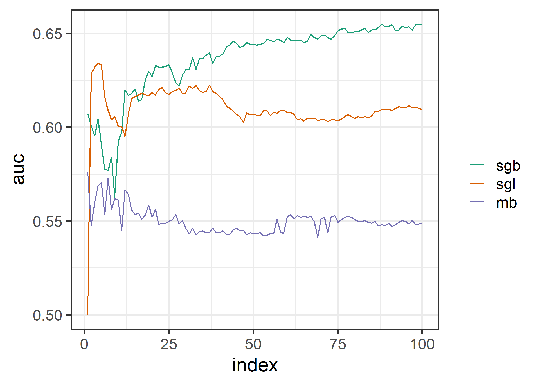
Figure 1: Genom data AUC paths averaged across 10 repeated resamples

fold

Table 1: Mean (mean), standard deviation (sd) and best (best) of all 100 models fitted for each model type (sgb, mb and sgl)

7.2 Agricultural data

Biomedical data are prominent examples of where sparse-group selection can be used. To show the variety of possible applications we analyze an agricultural dataset. Climate change impacts on the agricultural sector are well documented. The type and level of impacts are crop and region-specific. Not surprisingly, exposure to climate change makes many orchard farming communities in Chile and Tunisia vulnerable to climate change impacts. There are many susceptibility-related factors that may affect farm vulnerability to climatic impacts. A number of adaptation resources (measures/tools) are available to directly reduce the impact on farm operations or to reduce the number or sensitivity of susceptibility-related factors. The final objective is increased resilience of the farming communities. The dataset contains 24 outcome variables of interest that measure climate change vulnerability. The independent variables can be grouped into 7 groups depending on the construct the variable belongs to. Two group examples are social variables as well as the past adaptive measures. 801 farmers have been included in the study.

We use $\alpha\in(0,0.1,0.5,0.95,1)$ as mixing parameter for sgl and sgb. In addition, a mb model was fit. For each outcome variable we, randomly split 70 percent of the data into the training data and 30 percent into test data. We used this percentage since, for the training data we used a 10-fold cross-validation to estimate the optimal stopping parameter for the boosting models and the optimal $\lambda$ value for the sgl models. We used 100 $\lambda$ values and 10000 boosting iterations with a learning rate $\nu=0.2$. The remaining test data was used for the model evaluation. As in the previous section we used the auc as evaluation criterion, since all outcome variables are binary.

Referring to figure 7.1 and table LABEL:table:auc_vul it becomes apparent, that overall the models performed similarly regarding predictability. Overall the higher auc values were achieved for lower $\alpha$ values and sgb very marginally outperformed sgl for equal $\alpha$ values. The worst auc value of 0.677 was attained by model-based boosting compared to the highest of 0.692 attained by sgb with the alpha values of $0,0.1$ and $0.5$. Regarding computation time, for this specific dataset sgb was faster than sgl as 7.1 (c) suggests. It is important to note that the number of groups is relatively small compared to the number of observations. There were also substantial differences regarding the overall sparsity. In Figure 7.1 (b) it becomes apparent, that for higher $\alpha$ values, generally the overall sparsity increases for both sgl and sgb. Also relatively lower $\alpha$ values the sparsity of the sgl is higher compared to sgb and for relatively higher $\alpha$ values the opposite is true. In figure 3 we repeated the same setting with an equally spaced grid of 50 $\alpha$ values between zero and one and averaged the overall sparsity across the 25 variables. There seems to be a linear dependency between $\alpha$ and the sparsity for the sgl, and a sigmoid-like relationship for the sgb. From Lemma 1 we saw that the expectation of the residuals sum of squares (RSS) in $\mathcal{L}^{2}$-boosting is a linear function of the degrees of freedom, which is a linear function of $\alpha$ in the sgb. Using a normal approximation of the RSS one can see that the difference in RSS of an individual variable vs. a group-based variable follows also approximately a normal distribution. Then the selection probability of an individual variable vs. a group base-learner in one boosting iteration is the cumulative distribution function (cfd) of a normal distribution with expectation $2\alpha-1$ and some standard deviation also depending on $\alpha$ equated at zero. The selection of a new individual base-learner decreases the sparsity of the overall model by $\frac{1}{p}$ and the selection of a new group base-learner by $\frac{p_{g}}{p}$. This way we can see the sparsity after $m$ boosting steps can be seen as some generalized Bernoulli process, where the trials are not independent. For a big number of groups $G$ relative to the boosting steps $m$ we can then formulate this very rough approximation for the expected sparsity $s(\alpha)$ as depicted in Figure 3 $s(\alpha)\approx F_{2\alpha-1,\sigma(\alpha)}(0)\cdot\frac{1}{p}+\sum_{g=1}^{G}(1-F_{2\alpha-1,\sigma(\alpha)}(0))\cdot\frac{p_{g}}{p}$ is the expected sparsity depending on $\alpha$. This cdf shaped relationship between alpha and the sparsity seems to also translate to logistic regression and the use of cross-validation for early stopping as Figure 3 suggests.

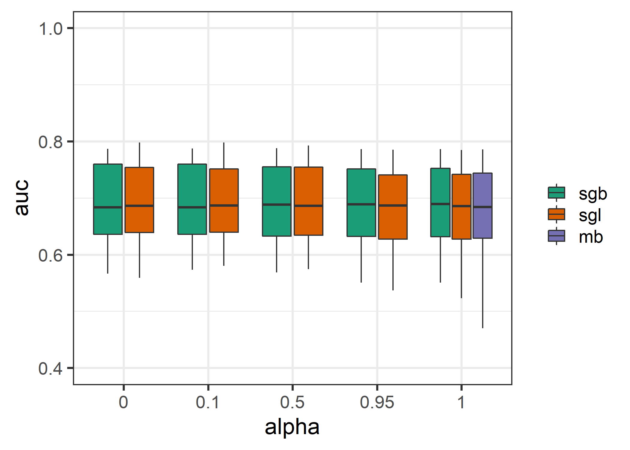
(a) AUC

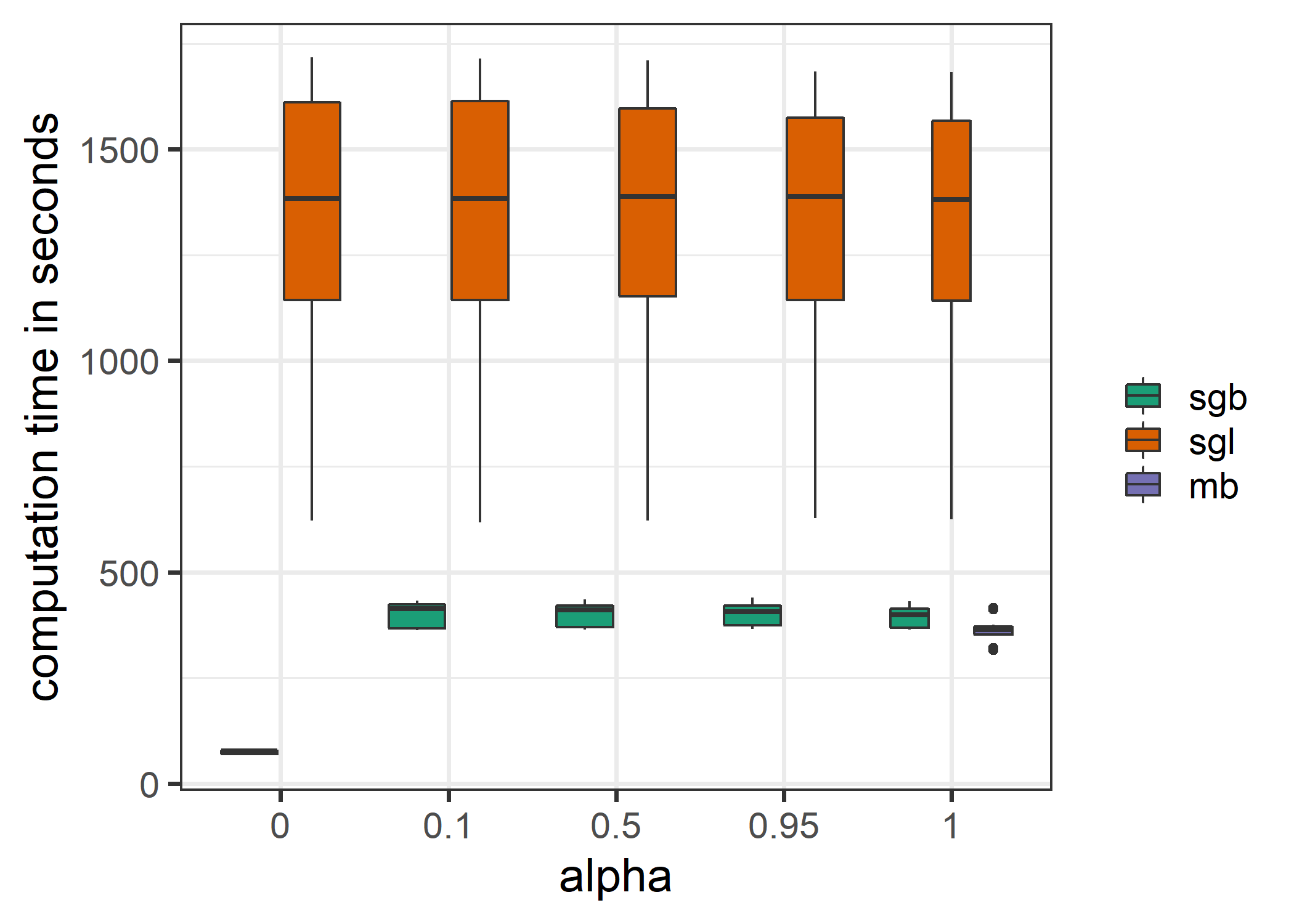
(c) Computation time

Figure 2: Comparison of 5 alpha values for various outcome variables in the dataset

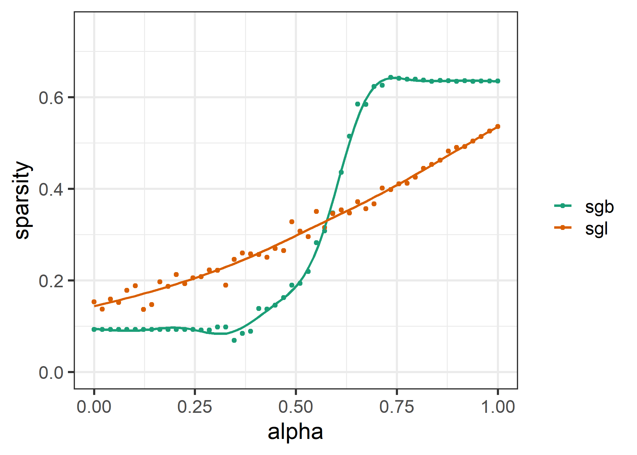
Figure 3: Sparsity curve depending on $\alpha$ averaged across various outcomes in the dataset

The covariate matrix X was simulated with different numbers of covariates, observations, correlation structures and groups. The response, y was set to

$$\sum_{g=1}^{G}X^{(g)}\beta^{(g)}+\sigma\epsilon.$$

Here, $\epsilon\sim\mathcal{N}(0,I)$. The signal-to-noise ratio was set to 2 through the value of $\sigma$. For the covariance structure of X we used a block correlation matrix to vary the within-group correlation as well as the between-group correlation. Always two groups contained effects and the number of groups $G$ was set to either 2 or 5, except in one scenario, where all groups and all variables have an effect. This leads to a changing between-group sparsity depending on the number of groups. We set $\beta^{(g)}=(1,1,0,...,0)$. The number of variables per group was set to two times the number of groups, which leads to a changing within-group sparsity depending on the number of groups. All models were tuned using a 10 fold cross-validation on training data and then evaluated with new simulated test data of the same structure. The tuned hyper-parameters were the number of iterations for all boosting models and the value of $\lambda$ or the sparse group lasso models. As the main evaluation criterion we used the mean squared error (MSE), defined as

$$\text{MSE}=\frac{1}{n}\sum_{i=1}^{n}\big{(}(y_{i}-f(X_{i\cdot})\big{)}^{2},$$

where $X_{i\cdot}$ is the $i$-th row of the design matrix. We also computed the proportion of correctly identified effects

$$\frac{\mathds{1}\sum_{j=1}^{p}[\widehat{\beta_{j}}=\beta_{j}]}{p}$$

With the code, the evaluation metrics for all 18 scenarios can be viewed. We would like to highlight a view metrics and results. First of all, we would like to note, that in all cases where generative groups were present, there was at least one $\alpha$, such that the MSE of the sparse group boosting was lower than the one of the standard boosting model. Referring to Figure 7.1, Tables 7.1, 7.1 and 7.1, the MSE of the lasso and of boosting were very comparable, which is in line with [hepp_approaches_2016]. In contrast to this, there are differences between the sgl and sgb. In the case of five groups and two groups with effect, those differences are in favor of the sgb. However, when all variables have an effect, the reverse is true. We would like to note, that when many variables have an effect, it can easily happen, that the boosting algorithm gets stopped out, meaning that the optimal stopping iteration is beyond the value set as maximum. Sgb does not perform well in this scenario, because the variables in bigger groups get regularized more than the variables in smaller groups. If now all variables have an effect, this leads to an inefficient attribution of shrinkage, and therefore to a longer convergence time. If the group structure is informative the converse is true. Apart from the predictability also the proportion of correctly identified parameters is very important. Regarding this property, the boosting models seem to outperform the lasso penalty-based models. The difference can be clearly seen in Table 7.1 and Figure 7.1, where no variable had any effect. In the applications, we already saw differences in the overall sparsity. There is a tendency for the sgb models to be sparser than their sgl counterparts. In this scenario, this tendency translates also in lower MSE. Regarding the computation time, there is a clear trend of group boosting being faster than the sparse group boosting and regular boosting, which is also slightly faster than sgb. This was to be expected, since overall in each boosting iteration more base-learners are being fitted in the sgb than the group boosting and regular boosting. Comparing the computation time sgl and sgb, the picture is not so clear. In the agricultural data, sgb was much faster than sgl and in the simulated data mostly the converse is true. We believe this has something with the number of observations (n) and the number of covariates (p) in the design matrix. The bigger the number of observations and the smaller the number of covariates, the faster sgb is compared to sgl. But this general tendency is also dependent on the implementation and may change in the future. There are efforts to improve both the computation time of sgl [ida_fast_2019] [zhang_efficient_2020] and boosting [staerk_randomized_2021]

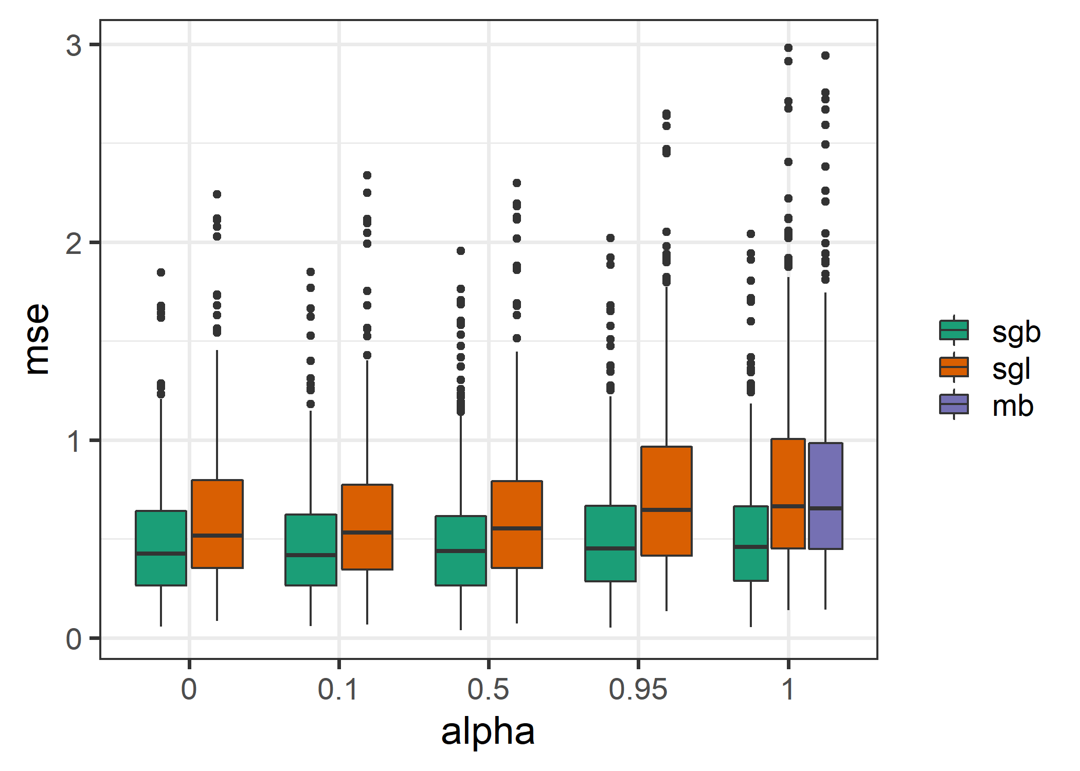
(a) n: 50, 5 groups, first 2 groups contain effect, uncorrelated predictors

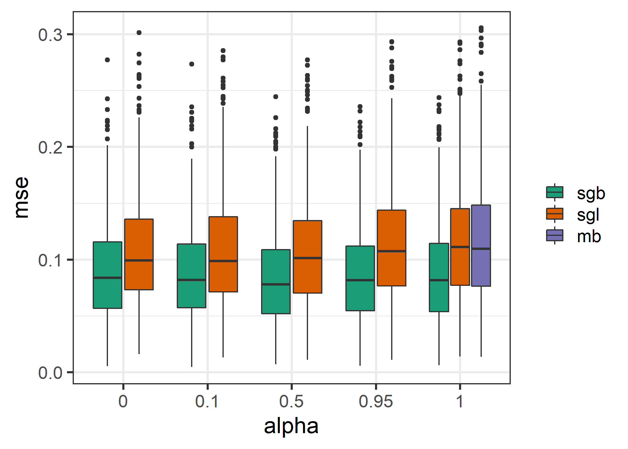
(c) n: 250, 5 groups, first 2 groups contain effect, uncorrelated predictors

Figure 4: Simulation results

alpha

Table 3: Simulation results: n: 50, 5 groups, first 2 groups contain effect, uncorrelated predictors (prop is the proportion of correct identification of the presence of effects)

alpha

Table 4: Simulation results: n: 250, 5 groups, first 2 groups contain effect, uncorrelated predictors (prop is the proportion of correct identification of the presence of effects)

alpha

Table 5: Simulation results: n: 250, 5 groups, uncorrelated predictors, all variables have an effect (prop is the proportion of correct identification of the presence of effects)

alpha

Table 6: Simulation results: n: 50, 5 groups, no effects, uncorrelated predictors (prop is the proportion of correct identification of the presence of effects)

The bibliography requires the ’biblatex’ package.

Appendix A Proof of Theorem 2

Proof.

Since the degrees of freedom of the individual base-learner is one, the ridge parameter is zero. So, for all $g\in\{1,2\}$ and $j\leq p_{g}$ we have

$$\\text{RSS}(x^{(g)}_{j}) (u-X^{(g)}_{j}\widehat{\beta}^{(g)}_{j})^{T}(u-X^{(g)}_{j}\widehat{\beta}^{(g)}_{j})$$

$$\ u(I-X^{(g)}_{j}((X^{(g)}_{j})^{T}X^{(g)}_{j})^{-1}(X^{(g)}_{j})^{T})u$$

$$\ \sim\chi^{2}_{n-1}.\$$

The first step follows form the fact that of the hat matrix is idempotent and the second step can be seen by using the singular value decomposition as well as the definition of the Chi squared definition. For g, h $\in\{1,2\}$ and $j\leq p_{g},k\leq p_{h}$ and $j\neq k$ if $gh$, we have

$$\P[\text{RSS}(x^{(g)}_{j})\leq\text{RSS}(x^{(h)}_{k})]P[\frac{\text{RSS}(x^{(g)}_{j})/(n-1)}{\text{RSS}(x^{(h)}_{k})/(n-1)}\leq 1]F(n-1,n-1),\$$

and

$$\P[\text{RSS}(x^{(h)}_{k})\leq\text{RSS}(x^{(g)}_{j})]P[\frac{\text{RSS}(x^{(h)}_{k})/(n-1)}{\text{RSS}(x^{(g)}_{j})/(n-1)}\leq 1]F(n-1,n-1),\$$

where $F$ is the cumulative distribution function of the $F$ distribution. Since the F distribution is well defined and continuous it follows, that

$$\P[\text{RSS}(x^{(h)}_{k})\leq\text{RSS}(x^{(g)}_{j})]0.5.\$$

Since all base-learners are independent if follows

$$\P\Big{[}\min_{j\in\{1,...,p_{1}\}}{\mathrm{RSS}(x^{(1)}_{j})}\leq\min_{k\in\{1,...,p_{2}\}}{\mathrm{RSS}(x^{(2)}_{j})}\Big{]}$$

$$\\sum_{j\in\{1,...,p_{1}\}}^{p_{1}}P\Big{[}\\mathrm{RSS}(x^{(1)}_{j})\min_{r\in\{1,2\},t\in\{1,...,p_{r}\}}\mathrm{RSS}(x^{(r)}_{t})\Big{]}$$

$$\\frac{p_{1}}{p_{1}+p_{2}}.\$$

∎

Appendix B Further simulation results

alpha

Table 7: Simulation results: n: 250, 5 groups, two group with effects, between-group correlation: 0.3, within-group correlation: 0. (prop is the proportion of correct identification of the presence of effects)

alpha

Table 8: Simulation results: n: 50, 5 groups, two groups with effects, between-group correlation: 0.3, within-group correlation: 0. (prop is the proportion of correct identification of the presence of effects)