Markov Chain Score Ascent:
A Unifying Framework of
Variational Inference with Markovian Gradients

Abstract

Minimizing the inclusive Kullback-Leibler (KL) divergence with stochastic gradient descent (SGD) is challenging since its gradient is defined as an integral over the posterior. Recently, multiple methods have been proposed to run SGD with biased gradient estimates obtained from a Markov chain. This paper provides the first non-asymptotic convergence analysis of these methods by establishing their mixing rate and gradient variance. To do this, we demonstrate that these methods–which we collectively refer to as Markov chain score ascent (MCSA) methods–can be cast as special cases of the Markov chain gradient descent framework. Furthermore, by leveraging this new understanding, we develop a novel MCSA scheme, parallel MCSA (pMCSA), that achieves a tighter bound on the gradient variance. We demonstrate that this improved theoretical result translates to superior empirical performance.

1 Introduction

Bayesian inference aims to analyze the posterior distribution of an unknown latent variable $\mathbf{z}$ from which data $\mathbf{x}$ is observed. By assuming a model $p\,(\mathbf{x}\,|\,\mathbf{z})$, the posterior $\pi\,(\mathbf{z})$ is given by Bayes’ rule such that $\pi\,(\mathbf{z})\propto{p\,(\mathbf{x}\,|\,\mathbf{z})\,p\,(\mathbf{z})}$ where $p\,(\mathbf{z})$ represents our prior belief on $\mathbf{z}$. Instead of working directly with $\pi$, variational inference (VI, blei_variational_2017) seeks a variational approximation $q\,(\mathbf{z};\mathbf{\lambda})\in\mathcal{Q}$, where $\mathcal{Q}$ is a variational family and $\mathbf{\lambda}$ are the variational parameters, that is the most similar to $\pi$ according to a discrepancy measure $d\,(\pi,\,q\,(\cdot;\mathbf{\lambda}))$.

The apparent importance of choosing the right discrepancy measure has led to a quest spanning a decade (NIPS2017_35464c84; NEURIPS2018_1cd138d0; NEURIPS2020_c928d86f; regli_alphabeta_2018; pmlr-v48-hernandez-lobatob16; NIPS2016_7750ca35; pmlr-v37-salimans15; pmlr-v97-ruiz19a; NEURIPS2021_05f971b5; NEURIPS2021_a1a609f1; bamler_perturbative_2017). So far, the exclusive (or reverse, backward) Kullback-Leibler (KL) divergence $d_{\mathrm{KL}}(q\left(\cdot;\mathbf{\lambda}\right)\parallel\pi)$ has seen “exclusive” use, partly because it is defined as an integral over $q\,(\mathbf{z};\mathbf{\lambda})$, which can be approximated efficiently. In contrast, the inclusive (or forward) KL is defined as an integral over $\pi$ as

$$d_{\mathrm{KL}}(\pi\parallel q\left(\cdot;\mathbf{\lambda}\right))=\int\pi\,(\mathbf{z})\log\frac{\pi\left(\mathbf{z}\right)}{q\,(\mathbf{z};\mathbf{\lambda})}\,d\mathbf{z}=\mathbb{E}_{\mathbfsf{z}\sim\pi\left(\cdot\right)}\left[\,\log\frac{\pi\left(\mathbfsf{z}\right)}{\,q\,(\mathbfsf{z};\mathbf{\lambda})}\,\right]$$

Since our goal is to approximate $\pi$ with $q\left(\cdot;\mathbf{\lambda}\right)$ but the inclusive KL involves an integral over $\pi$, we end up facing a chicken-and-egg problem. Despite this challenge, the inclusive KL has consistently drawn attention due to its statistical properties, such as better uncertainty estimates due to its mass covering property (minka2005divergence; mackay_local_2001; trippe_overpruning_2017).

Recently, NEURIPS2020_b2070693; pmlr-v124-ou20a have respectively proposed Markovian score climbing (MSC) and joint stochastic approximation (JSA). These methods minimize the inclusive KL using stochastic gradient descent (SGD, robbins_stochastic_1951), where the gradients are estimated using a Markov chain. The Markov chain kernel $K_{\mathbf{\lambda}_{t}}\left(\mathbf{z}_{t},\cdot\right)$ is $\pi$-invariant (robert_monte_2004) and is chosen such that it directly takes advantage of the current variational approximation $q\left(\cdot;\mathbf{\lambda}_{t}\right)$. Thus, the quality of the gradients improves over time as the KL divergence decreases. Still, the gradients are non-asymptotically biased and Markovian across adjacent iterations, which sharply contrasts MSC and JSA from classical black-box VI (pmlr-v33-ranganath14; JMLR:v18:16-107), where the gradients are unbiased and independent. While NEURIPS2020_b2070693 have shown the convergence of MSC through the work of gu_stochastic_1998, this result is only asymptotic and does not provide practical insight into the performance of MSC.

In this paper, we address these theoretical gaps by casting MSC and JSA into a general framework we call Markov chain score ascent (MCSA), which we show is a special case of Markov chain gradient descent (MCGD, duchi_ergodic_2012). This enables the application of the non-asymptotic convergence results of MCGD (duchi_ergodic_2012; NEURIPS2018_1371bcce; pmlr-v99-karimi19a; doan_finitetime_2020; doan_convergence_2020; Xiong_Xu_Liang_Zhang_2021; debavelaere_convergence_2021). For MCGD methods, the fundamental properties affecting the convergence rate are the ergodic convergence rate ($\rho$) of the MCMC kernel and the gradient variance ($G$). We analyze $\rho$ and $G$ of MSC and JSA, enabling their practical comparison given a fixed computational budget ($N$). Furthermore, based on the recent insight that the mixing rate does not affect the convergence rate of MCGD (doan_convergence_2020; doan_finitetime_2020), we propose a novel scheme, parallel MCSA (pMCSA), which achieves lower variance by trading off the mixing rate. We verify our theoretical analysis through numerical simulations and compare MSC, JSA, and pMCSA on general Bayesian inference problems. Our experiments show that our proposed method outperforms previous MCSA approaches.

Contribution Summary

1. We provide the first non-asymptotic theoretical analysis of two recently proposed inclusive KL minimization methods (Section 4), MSC (Sections 4.2 and 4.2) and JSA (Section 4.3).

2. To do this, we show that both methods can be viewed as what we call “Markov chain score ascent” (MCSA) methods (Section 3), which are a special case of MCGD (Section 3.1).

3. In light of this, we develop a novel MCSA method which we call parallel MCSA (pMCSA, Section 5) that achieves lower gradient variance (Section 5.1).

4. We demonstrate that the improved theoretical performance of pMCSA translates to superior empirical performance across a variety of Bayesian inference tasks (LABEL:section:eval).

2 Background

2.1 Inclusive Kullback-Leibler Minimization with Stochastic Gradients

VI with SGD

The goal of VI is to find the optimal variational parameters $\mathbf{\lambda}$ identifying $q\left(\cdot;\mathbf{\lambda}\right)\in\mathcal{Q}$ that minimizes some discrepancy measure $D\left(\pi,q\left(\cdot;\mathbf{\lambda}\right)\right)$. A typical way to perform VI is to use stochastic gradient descent (SGD, robbins_stochastic_1951), provided that the optimization objective provides unbiased gradient estimates $\mathbf{g}\,(\mathbf{\lambda})$ such that we can repeat the update

$$\mathbf{\lambda}_{t}=\mathbf{\lambda}_{t-1}-\gamma_{t}\,\mathbf{g}\left(\mathbf{\lambda}_{t-1}\right),$$

where $\gamma_{1},\ldots,\gamma_{T}$ is a stepsize schedule.

Inclusive KL Minimization with SGD

For inclusive KL minimization, $\mathbf{g}$ should be set as

$$\mathbf{g}\left(\mathbf{\lambda}\right)=\nabla_{\mathbf{\lambda}}d_{\mathrm{KL}}(\pi\parallel q\left(\cdot;\mathbf{\lambda}\right))=\nabla_{\mathbf{\lambda}}\mathbb{H}\left[\pi,q\left(\cdot;\mathbf{\lambda}\right)\right]=-\mathbb{E}_{\mathbfsf{z}\sim\pi\left(\cdot\right)}\left[\,\mathbf{s}\,(\mathbf{\lambda};\mathbfsf{z})\,\right],$$

where $\mathbb{H}\left[\pi,q\left(\cdot;\mathbf{\lambda}\right)\right]$ is the cross-entropy between $\pi$ and $q\left(\cdot;\mathbf{\lambda}\right)$, which shows the connection with cross-entropy methods (deboer_tutorial_2005), and $\mathbf{s}\,(\mathbf{\lambda};\mathbf{z})=\nabla_{\mathbf{\lambda}}\log q\,(\mathbf{z};\mathbf{\lambda})$ is known as the score gradient. Since inclusive KL minimization with SGD is equivalent to ascending towards the direction of the score, NEURIPS2020_b2070693 coined the term score climbing. To better conform with the optimization literature, we instead call this approach score ascent as in gradient ascent.

2.2 Markov Chain Gradient Descent

Overview of MCGD

Markov chain gradient descent (MCGD, duchi_ergodic_2012; NEURIPS2018_1371bcce) is a family of algorithms that minimize a function $f$ defined as $f\left(\mathbf{\lambda}\right)=\int f\left(\mathbf{\lambda},\mathbf{\eta}\right)\,\Pi\left(d\mathbf{\eta}\right)$, where $\mathbf{\eta}$ is random noise, and $\Pi\left(d\mathbf{\eta}\right)$ is its probability measure. MCGD repeats the steps

$$\mathbf{\lambda}_{t+1}=\mathbf{\lambda}_{t}-\gamma_{t}\,\mathbf{g}\left(\mathbf{\lambda}_{t},\mathbf{\eta}_{t}\right),\quad\mathbfsf{\eta}_{t}\sim P_{\mathbf{\lambda}_{t-1}}\left(\mathbf{\eta}_{t-1},\cdot\right),$$ (1)

where $P_{\mathbf{\lambda}_{t-1}}$ is a $\Pi$-invariant Markov chain kernel that may depend on $\mathbf{\lambda}_{t-1}$. The noise of the gradient is Markovian and non-asymptotically biased, departing from vanilla SGD. Non-asymptotic convergence of this general algorithm has recently started to gather attention as by duchi_ergodic_2012; NEURIPS2018_1371bcce; pmlr-v99-karimi19a; doan_finitetime_2020; doan_convergence_2020; debavelaere_convergence_2021.

Applications of MCGD

MCGD encompasses an extensive range of problems, including distributed optimization (ram_incremental_2009), reinforcement learning (tadic_asymptotic_2017; doan_convergence_2020; Xiong_Xu_Liang_Zhang_2021), and expectation-minimization (pmlr-v99-karimi19a), to name a few. This paper extends this list with inclusive KL VI through the MCSA framework.

3 Markov Chain Score Ascent

First, we develop Markov chain score ascent (MCSA), a framework for inclusive KL minimization with MCGD. This framework will establish the connection between MSC/JSA and MCGD.

3.1 Markov Chain Score Ascent as a Special Case of Markov Chain Gradient Descent

As shown in Equation 1, the basic ingredients of MCGD are the target function $f\left(\mathbf{\lambda},\eta\right)$, the gradient estimator $\mathbf{g}\left(\mathbf{\lambda},\eta\right)$, and the Markov chain kernel $P_{\mathbf{\lambda}}\left(\eta,\cdot\right)$. Obtaining MCSA from MCGD boils down to designing $\mathbf{g}$ and $P_{\mathbf{\lambda}}$ such that $f\left(\mathbf{\lambda}\right)=d_{\mathrm{KL}}(\pi\parallel q\left(\cdot;\mathbf{\lambda}\right))$. The following proposition provides sufficient conditions on $\mathbf{g}$ and $P_{\mathbf{\lambda}}$ to achieve this goal.

proposition Let $\mathbf{\eta}=\left(\mathbf{z}^{(1)},\mathbf{z}^{(2)},\ldots,\mathbf{z}^{(N)}\right)$ and a Markov chain kernel $P_{\mathbf{\lambda}}\left(\mathbf{\eta},\cdot\right)$ be $\Pi$-invariant where $\Pi$ is defined as

$$\Pi\left(\mathbf{\eta}\right)=\pi\left(\mathbf{z}^{(1)}\right)\,\pi\left(\mathbf{z}^{(2)}\right)\times\ldots\times\pi\left(\mathbf{z}^{(N)}\right).$$

Then, by defining the objective function $f$ and the gradient estimator $\mathbf{g}$ to be

$$\textstyle f\left(\mathbf{\lambda},\mathbf{\eta}\right)=-\frac{1}{N}\sum^{N}_{n=1}\log q\left(\mathbf{z}^{(n)};\mathbf{\lambda}\right)-\mathbb{H}\left[\,\pi\,\right]\quad\text{and}\quad\mathbf{g}\left(\mathbf{\lambda},\mathbf{\eta}\right)=-\frac{1}{N}\sum^{N}_{n=1}\mathbf{s}\left(\mathbf{z}^{(n)};\mathbf{\lambda}\right),$$

where $\mathbb{H}\left[\,\pi\,\right]$ is the entropy of $\pi$, MCGD results in inclusive KL minimization as

$$\mathbb{E}_{\Pi}\left[\,f\left(\mathbf{\lambda},\mathbfsf{\eta}\right)\,\right]=d_{\mathrm{KL}}(\pi\parallel q\left(\cdot;\mathbf{\lambda}\right))\quad\text{and}\quad\mathbb{E}_{\Pi}\left[\,\mathbf{g}\left(\mathbf{\lambda},\mathbfsf{\eta}\right)\,\right]=\nabla_{\mathbf{\lambda}}d_{\mathrm{KL}}(\pi\parallel q\left(\cdot;\mathbf{\lambda}\right)).$$

For notational convenience, we define the shorthand

$$\pi\left(\mathbf{z}^{(1:N)}\right)=\pi\left(\mathbf{z}^{(1)}\right)\,\pi\left(\mathbf{z}^{(2)}\right)\times\ldots\times\pi\left(\mathbf{z}^{(N)}\right).$$

Then,

$$\mathbb{E}_{\Pi}\left[\,f\left(\mathbf{\lambda},\mathbfsf{\eta}\right)\,\right]$$

$$\quad=\int\left(-\frac{1}{N}\sum^{N}_{n=1}\log q\left(\mathbf{z}^{(n)};\mathbf{\lambda}\right)-\mathbb{H}\left[\,\pi\,\right]\right)\,\pi\left(\mathbf{z}^{(1:N)}\right)\,d\mathbf{z}^{(1:N)}$$

$$\quad=\int\left(-\frac{1}{N}\sum^{N}_{n=1}\log q\left(\mathbf{z}^{(n)};\mathbf{\lambda}\right)\right)\,\pi\left(\mathbf{z}^{(1:N)}\right)\,d\mathbf{z}^{(1:N)}-\mathbb{H}\left[\,\pi\,\right]$$

$$\quad=\frac{1}{N}\sum^{N}_{n=1}\left\{\int\big{(}-\log q\,(\,\mathbf{z}^{(n)};\mathbf{\lambda}\,)\,\big{)}\,\pi\left(\mathbf{z}^{(1:N)}\right)\,d\mathbf{z}^{(1:N)}\right\}-\mathbb{H}\,[\,\pi\,]$$

$$\quad=\frac{1}{N}\sum^{N}_{n=1}\int\big{(}-\log q\,(\,\mathbf{z}^{(n)};\mathbf{\lambda}\,)\,\big{)}\,\pi\left(\mathbf{z}^{(n)}\right)\,d\mathbf{z}^{(n)}-\mathbb{H}\,[\,\pi\,] \mathbf{z}^{(m)} m\neq n$$ Marginalized for all

$$\quad=\frac{1}{N}\sum^{N}_{n=1}\int\big{(}-\log q\,(\,\mathbf{z}^{(n)};\mathbf{\lambda}\,)+\log\pi\left(\mathbf{z}^{(n)}\right)\,\big{)}\,\pi\left(\mathbf{z}^{(n)}\right)\,d\mathbf{z}^{(n)} \mathbb{H}\left[\pi\right]$$ Definition of

$$\quad=\frac{1}{N}\sum^{N}_{n=1}\int\pi\left(\mathbf{z}^{(n)}\right)\,\log\frac{\pi\left(\mathbf{z}^{(n)}\right)}{q\,(\,\mathbf{z}^{(n)};\mathbf{\lambda}\,)}\,d\mathbf{z}^{(n)}$$

$$\quad=\frac{1}{N}\sum^{N}_{n=1}d_{\mathrm{KL}}(\pi\parallel q\left(\cdot;\mathbf{\lambda}\right)) d_{\text{KL}}$$ Definition of

$$\quad=d_{\mathrm{KL}}(\pi\parallel q\left(\cdot;\mathbf{\lambda}\right)).$$ (2)

For $\mathbb{E}_{\Pi}\left[\,\mathbf{g}\left(\mathbf{\lambda},\mathbfsf{\eta}\right)\,\right]$, note that

$$\nabla_{\mathbf{\lambda}}f\left(\mathbf{\lambda},\mathbf{\eta}\right)=-\frac{1}{N}\sum^{N}_{n=1}\nabla_{\mathbf{\lambda}}\log q\left(\mathbf{z}^{(n)};\mathbf{\lambda}\right)=-\frac{1}{N}\sum^{N}_{n=1}\mathbf{s}\left(\mathbf{z}^{(n)};\mathbf{\lambda}\right)=\mathbf{g}\left(\mathbf{\lambda},\mathbf{\eta}\right).$$ (3)

Therefore, it suffices to show that

$$\nabla_{\mathbf{\lambda}}d_{\mathrm{KL}}(\pi\parallel q\left(\cdot;\mathbf{\lambda}\right)) =\nabla_{\mathbf{\lambda}}\mathbb{E}_{\Pi}\left[\,f\left(\mathbf{\lambda},\mathbfsf{\eta}\right)\,\right]$$

$$=\mathbb{E}_{\Pi}\left[\,\nabla_{\mathbf{\lambda}}f\left(\mathbf{\lambda},\mathbfsf{\eta}\right)\,\right]$$ Leibniz derivative rule

$$=\mathbb{E}_{\Pi}\left[\,\mathbf{g}\left(\mathbf{\lambda},\mathbfsf{\eta}\right)\,\right].$$

Table 1: Convergence Rates of MCGD Algorithms

Algorithm	Stepsize Rule	Gradient Assumption	Rate	Reference
Mirror Descent1	$\gamma_{t}=\gamma/\sqrt{t}$	$\mathbb{E}\left[\,{\|\,\mathbf{g}\left(\mathbfsf{\lambda},\mathbfsf{\eta}\right)\,\|}_{*}^{2}\mid\mathcal{F}_{t-1}\,\right]<G^{2}$	$\mathcal{O}\left(\frac{G^{2}\log T}{\log\rho^{-1}\sqrt{T}}\right)$	duchi_ergodic_2012
				Corollary 3.5
1-5 SGD-Nesterov2	$\gamma_{t}=2/(t+1)$	${\|\,\mathbf{g}\left(\mathbfsf{\lambda},\mathbfsf{\eta}\right)\|}_{2}<G$	$\mathcal{O}\left(\frac{G^{2}\log T}{\sqrt{T}}\right)$	doan_convergence_2020
	$\beta_{t}=\frac{1}{2\,L\sqrt{t+1}}$			Theorem 2
1-5 SGD3	$\gamma_{t}=\gamma/t$	${\|\,\mathbf{g}\left(\mathbfsf{\lambda},\mathbfsf{\eta}\right)\|}_{*}<G\left({\left\lVert\,\mathbf{\lambda}\,\right\rVert}_{2}+1\right)$	$\mathcal{O}\left(\frac{G^{2}\log T}{T}\right)$	doan_finitetime_2020
	$\gamma=\min\{\nicefrac{{1}}{{2\,L}},\nicefrac{{2L}}{{\mu}}\}$			Theorem 1,2

• Notation: ¹$\mathcal{F}_{t}$ is the $\sigma$-field formed by the iterates $\mathbf{\eta}_{t}$ up to the $t$th MCGD iteration, ${\left\lVert\,\mathbf{x}\,\right\rVert}_{*}$ is the dual norm of $\mathbf{x}$; ²$\beta_{t}$ is the stepsize of the momentum; ²³$L$ is the Lipschitz smoothness constant; ³$\mu$ is the strong convexity constant.

This simple connection between MCGD and VI paves the way toward the non-asymptotic analysis of JSA and MSC. Note that $N$ here can be regarded as the computational budget of each MCGD iteration since the cost of (i) generating the Markov chain samples $\mathbf{z}^{(1)},\ldots,\mathbf{z}^{(N)}$ and (ii) computing the gradient $\mathbf{g}$ will linearly increase with $N$.

In addition, the MCGD framework often assumes $P$ to be geometrically ergodic. An exception is the analysis of debavelaere_convergence_2021 where they work with polynomially ergodic kernels.

Assumption 1.

(Markov chain kernel) The Markov chain kernel $P$ is geometrically ergodic as $${d_{\mathrm{TV}}\left(P_{\mathbf{\lambda}}^{n}\left(\mathbf{\eta},\cdot\right),\Pi\right)}\leq C\,\rho^{n}$$ for some positive constant $C$.

3.2 Non-Asymptotic Convergence of Markov Chain Score Ascent

Non-Asymptotic Convergence

Through Section 3.1, Assumption 1 and some technical assumptions on the objective function, we can apply the existing convergence results of MCGD to MCSA. Section 3.1 provides a list of relevant results. Apart from properties of the objective function (such as Lipschitz smoothness), the convergence rates are stated in terms of the gradient bound $G$, kernel mixing rate $\rho$, and the number of MCGD iterations $T$. We focus on $G$ and $\rho$ as they are closely related to the design choices of different MCSA algorithms.

Convergence and the Mixing Rate $\rho$

duchi_ergodic_2012 was the first to provide an analysis of the general MCGD setting. Their convergence rate is dependent on the mixing rate through the $1/\log\rho^{-1}$ term. For MCSA, this result is overly conservative since, on challenging problems, mixing can be slow such that $\rho\approx 1$. Fortunately, doan_convergence_2020; doan_finitetime_2020 have recently shown that it is possible to obtain a rate independent of the mixing rate $\rho$. For example, in the result of doan_finitetime_2020, the influence of $\rho$ decreases in a rate of $\mathcal{O}\left(\nicefrac{{1}}{{T^{2}}}\right)$. This observation is critical since it implies that trading a “slower mixing rate” for “lower gradient variance” could be profitable. We exploit this observation in our novel MCSA scheme in Section 5.

Gradient Bound $G$

Except for doan_finitetime_2020, most results assume that the gradient is bounded for $\forall\mathbf{\eta},\mathbf{\lambda}$ as ${\|\mathbf{g}\left(\mathbf{\lambda},\mathbf{\eta}\right)\|}<G$. Admittedly, this condition is strong, but it is similar to the bounded variance assumption $\mathbb{E}\,[{\left\lVert\,\mathbf{g}\,\right\rVert}^{2}]<G^{2}$ used in vanilla SGD, which is also known to be strong as it contradicts strong convexity (pmlr-v80-nguyen18c). Nonetheless, assuming $G$ can have practical benefits beyond theoretical settings. For example, pmlr-v108-geffner20a use $G$ to compare the performance different VI gradient estimators. In a similar spirit, we will obtain the gradient bound $G$ of different MCSA algorithms and compare their theoretical performance.

4 Demystifying Prior Markov Chain Score Ascent Methods

In this section, we will show that MSC and JSA both qualify as MCSA methods. Furthermore, we establish (i) the mixing rate of their implicitly defined kernel $P$ and (ii) the upper bound on their gradient variance. This will provide insight into their practical non-asymptotic performance.

4.1 Technical Assumptions

To cast previous methods into MCSA, we need some technical assumptions.

Assumption 2.

(Bounded importance weight) The importance weight ratio $w\left(\mathbf{z}\right)=\pi\left(\mathbf{z}\right)/q\left(\mathbf{z};\mathbf{\lambda}\right)$ is bounded by some finite constant as $w^{*}<\infty$ for all $\mathbf{\lambda}\in\Lambda$ such that $r=\left(1-1/w^{*}\right)<1$.

This assumption is necessary to ensure Assumption 1, and can be practically ensured by using a variational family with heavy tails (NEURIPS2018_25db67c5) or using a defensive mixture (hesterberg_weighted_1995; holden_adaptive_2009) as

$$q_{\text{def.}}\left(\mathbf{z};\mathbf{\lambda}\right)=\alpha\,q\left(\mathbf{z};\mathbf{\lambda}\right)+(1-\alpha)\,\nu\left(\mathbf{z}\right),$$

where $0<\alpha<1$ and $\nu\left(\cdot\right)$ is a heavy tailed distribution such that $\sup_{\mathbf{z}\in\mathcal{Z}}\pi\left(\mathbf{z}\right)/\nu\left(\mathbf{z}\right)<\infty$. Note that $q_{\text{def.}}$ is only used in the Markov chain kernels and $q\left(\cdot;\mathbf{\lambda}\right)$ is still the output of the VI procedure. While these tricks help escape slowly mixing regions, this benefit quickly vanishes as $\lambda$ converges. Therefore, ensuring Assumption 2 seems unnecessary in practice unless we absolutely care about ergodicity. (Think of the adaptive MCMC setting for example. holden_adaptive_2009; pmlr-v151-brofos22a).

Model (Variational Family) Misspecification and $w^{*}$

Note that $w^{*}$ is bounded below exponentially by the inclusive KL as shown in Section 4.2. Therefore, $w^{*}$ will be large (i) in the initial steps of VI and (ii) under model (variational family) misspecification.

Assumption 3.

(Bounded Score) The score gradient is bounded for $\forall\mathbf{\lambda}\in\Lambda$ and $\forall\mathbf{z}\in\mathcal{Z}$ such that ${\left\lVert\,\mathbf{s}\left(\mathbf{\lambda};\mathbf{z}\right)\,\right\rVert}_{2}\leq L$ for some finite constant $L>0$.

Although this assumption is strong, it enables us to compare the gradient variance of MCSA methods. We empirically justify the bounds obtained using Assumption 3 in LABEL:section:simulation.

4.2 Markovian Score Climbing

MSC (Algorithm 4 in Appendix B) is a simple instance of MCSA where $\mathbf{\eta}_{t}=\mathbf{z}_{t}$ and $P_{\mathbf{\lambda}_{t}}=K_{\mathbf{\lambda}_{t}}$ is the conditional importance sampling (CIS) kernel (originally proposed by andrieu_uniform_2018) where the proposals are generated from $q\left(\cdot;\mathbf{\lambda}_{t}\right)$. Although MSC uses only a single sample for the Markov chain, the CIS kernel internally operates $N-1$ proposals. Therefore, $N$ in MSC has a different meaning, but it still indicates the computational budget.

[all end]proposition The maximum importance weight $w^{*}=\sup_{\mathbf{z}}w\left(\mathbf{z}\right)=\sup_{\mathbf{z}}\pi\left(\mathbf{z}\right)/q\left(\mathbf{z};\mathbf{\lambda}\right)$ is bounded below exponentially by the KL divergence as

$$\exp\left(d_{\mathrm{KL}}(\pi\parallel q\left(\cdot;\mathbf{\lambda}\right))\right)<w^{*}.$$

$$d_{\mathrm{KL}}(\pi\parallel q\left(\cdot;\mathbf{\lambda}\right)) =\mathbb{E}_{\mathbfsf{z}\sim\pi\left(\cdot\right)}\left[\,\log\frac{\pi\left(\mathbfsf{z}\right)}{q\left(\mathbfsf{z};\mathbf{\lambda}\right)}\,\right] d_{\text{KL}}$$ Definition of

$$\leq\log\mathbb{E}_{\mathbfsf{z}\sim\pi\left(\cdot\right)}\left[\,\frac{\pi\left(\mathbfsf{z}\right)}{q\left(\mathbfsf{z};\mathbf{\lambda}\right)}\,\right]$$ Jensen’s inequality

$$\leq\log\mathbb{E}_{\mathbfsf{z}\sim\pi\left(\cdot\right)}\left[\,w^{*}\,\right]$$

$$=\log w^{*}.$$

[all end]lemma For the probability measures $p_{1},\ldots,p_{N}$ and $q_{1},\ldots,q_{N}$ defined on a measurable space $(\mathsf{X},\mathcal{A})$ and an arbitrary set $A\in\mathcal{A}$,

$${\left|\,\int_{A^{N}}p_{1}\left(dx_{1}\right)p_{2}\left(dx_{2}\right)\times\ldots\times p_{N}\left(dx_{N}\right)-q_{1}\left(dx_{1}\right)q_{2}\left(dx_{2}\right)\times\ldots\times q_{N}\left(dx_{N}\right)\,\right|}$$

$$\qquad\leq\sum_{n=1}^{N}{\left|\,\int_{A}p_{n}\left(dx_{n}\right)-q_{n}\left(dx_{n}\right)\,\right|}$$

By using the following shorthand notations

$$p_{(1:N)}\left(dx_{(1:N)}\right) =p_{1}\left(dx_{1}\right)p_{2}\left(dx_{2}\right)\times\ldots\times p_{N}\left(dx_{N}\right)$$

$$q_{(1:N)}\left(dx_{(1:N)}\right) =q_{1}\left(dx_{1}\right)q_{2}\left(dx_{2}\right)\times\ldots\times q_{N}\left(dx_{N}\right),$$

the result follows from induction as

$${\left|\,\int_{A^{N}}p_{(1:N)}\left(dx_{(1:N)}\right)-q_{(1:N)}\left(dx_{(1:N)}\right)\,\right|}$$

$$\quad=\Bigg{|}\;\left(\int_{A}p_{1}\left(dx_{1}\right)-q_{1}\left(dx_{1}\right)\right)\,\int_{A^{N-1}}p_{(2:N)}\left(dx_{(2:N)}\right)$$

$$\qquad\quad+\int_{A}q_{1}\left(dx_{1}\right)\,{\left(\int_{A^{N-1}}p_{(2:N)}\left(dx_{(2:N)}\right)-q_{(2:N)}\left(dx_{(2:N)}\right)\right)}\;\Bigg{|}$$

$$\quad\leq\Bigg{|}\int_{A}p_{1}\left(dx_{1}\right)-q_{1}\left(dx_{1}\right)\Bigg{|}\;\int_{A^{N-1}}p_{(2:N)}\left(dx_{(2:N)}\right)$$

$$\qquad\quad+\int_{A}q_{1}\left(dx_{1}\right)\,{\Bigg{|}\;\int_{A^{N-1}}p_{(2:N)}\left(dx_{(2:N)}\right)-q_{(2:N)}\left(dx_{(2:N)}\right)}\;\Bigg{|}$$ Triangle inequality

$$\quad\leq\Bigg{|}\int_{A}p_{1}\left(dx_{1}\right)-q_{1}\left(dx_{1}\right)\Bigg{|}\;$$

$$\qquad\quad+{\Bigg{|}\;\int_{A^{N-1}}p_{(2:N)}\left(dx_{(2:N)}\right)-q_{(2:N)}\left(dx_{(2:N)}\right)}\;\Bigg{|}. p_{n}\left(A\right),q_{n}\left(A\right)\leq 1$$ Applied

[all end]lemma Let $\mathbfsf{g}$ be a vector-valued, biased estimator of $\mathbf{\mu}$, where the bias is denoted as $\mathsf{Bias}\left[\mathbfsf{g}\right]={\left\lVert\,\mathbb{E}\mathbfsf{g}-\mathbf{\mu}\,\right\rVert}_{2}$ and the mean-squared error is denoted as $\mathsf{MSE}\left[\mathbfsf{g}\right]=\mathbb{E}{\left\lVert\,\mathbfsf{g}-\mathbf{\mu}\,\right\rVert}_{2}^{2}$. Then, the second moment of $\mathbfsf{g}$ is bounded as

1. $\mathbb{E}{\left\lVert\,\mathbfsf{g}\,\right\rVert}^{2}_{2}\leq\mathbb{V}{\mathbfsf{g}}+{\mathsf{Bias}\left[\mathbfsf{g}\right]}^{2}+2\,\mathsf{Bias}\left[\mathbfsf{g}\right]{\left\lVert\,\mathbf{\mu}\,\right\rVert}_{2}+{\left\lVert\,\mathbf{\mu}\,\right\rVert}^{2}_{2},$

2. $\mathbb{E}{\left\lVert\,\mathbfsf{g}\,\right\rVert}^{2}_{2}\leq\mathsf{MSE}\left[{\mathbfsf{g}}\right]+2\,\mathsf{Bias}\left[\mathbfsf{g}\right]{\left\lVert\,\mathbf{\mu}\,\right\rVert}_{2}+{\left\lVert\,\mathbf{\mu}\,\right\rVert}^{2}_{2},$

where $\mathbb{V}\mathbfsf{g}=\mathbb{E}{\left\lVert\,\mathbfsf{g}-\mathbb{E}\mathbf{g}\,\right\rVert}_{2}^{2}$ is the variance of the estimator. ❶ follows from the decomposition

$$\mathbb{E}\left[\,{\left\lVert\,\mathbfsf{g}\,\right\rVert}^{2}_{2}\,\right] \;=\mathbb{V}{\mathbfsf{g}}+{\left\lVert\,\mathbb{E}{\mathbfsf{g}}\,\right\rVert}_{2}^{2}$$

$$\;=\mathbb{V}{\mathbfsf{g}}+{\left\lVert\,\mathbb{E}{\mathbfsf{g}}-\mathbf{\mu}+\mathbf{\mu}\,\right\rVert}_{2}^{2}$$

$$\;=\mathbb{V}{\mathbfsf{g}}+{\left\lVert\,\mathbb{E}{\mathbfsf{g}}-\mathbf{\mu}\,\right\rVert}_{2}^{2}+2\,{\left(\mathbb{E}\mathbfsf{g}-\mathbf{\mu}\right)}^{\top}\mathbf{\mu}+{\left\lVert\,\mathbf{\mu}\,\right\rVert}^{2}_{2}$$ Expanded quadratic

$$\;\leq\mathbb{V}{\mathbfsf{g}}+{\left\lVert\,\mathbb{E}{\mathbfsf{g}}-\mathbf{\mu}\,\right\rVert}_{2}^{2}+2\,{\left\lVert\,\mathbb{E}{\mathbfsf{g}}-\mathbf{\mu}\,\right\rVert}_{2}{\left\lVert\,\mathbf{\mu}\,\right\rVert}_{2}+{\left\lVert\,\mathbf{\mu}\,\right\rVert}_{2}^{2}$$ Cauchy-Shwarz inequality

$$\;=\mathbb{V}{\mathbfsf{g}}+{\mathsf{Bias}\left[\mathbfsf{g}\right]}^{2}+2\,\mathsf{Bias}\left[\mathbfsf{g}\right]{\left\lVert\,\mathbf{\mu}\,\right\rVert}_{2}+{\left\lVert\,\mathbf{\mu}\,\right\rVert}_{2}^{2}.$$ Definition of bias

Meanwhile, by the well-known bias-variance decomposition formula of the mean-squared error, ❷ directly follows from ❶.

theorem MSC (NEURIPS2020_b2070693) is obtained by defining

$$P_{\lambda}^{k}\left(\mathbf{\eta},d\mathbf{\eta}^{\prime}\right)=K_{\lambda}^{k}\left(\mathbf{z},d\mathbf{z}^{\prime}\right)$$

with $\mathbf{\eta}_{t}=\mathbf{z}_{t}$, where $K_{\mathbf{\lambda}}\left(\mathbf{z},\cdot\right)$ is the CIS kernel with $q_{\text{def.}}\left(\cdot;\mathbf{\lambda}\right)$ as its proposal distribution. Then, given Assumption 2 and 3, the mixing rate and the gradient bounds are given as

$$\textstyle{d_{\mathrm{TV}}\left(P_{\mathbf{\lambda}}^{k}\left(\mathbf{\eta},\cdot\right),\Pi\right)}\leq{\left(1-\frac{N-1}{2w^{*}+N-2}\right)}^{k}\quad\text{and}\quad{\small\mathbb{E}\left[\,{\lVert\mathbfsf{g}_{t,\text{MSC}}\rVert}^{2}\,\middle|\,\mathcal{F}_{t-1}\,\right]\leq L^{2},}$$

where $w^{*}=\sup_{\mathbf{z}}\pi\left(\mathbf{z}\right)/q_{\text{def.}}\left(\mathbf{z};\mathbf{\lambda}\right)$. MSC is described in Algorithm 4. At each iteration, it performs a single MCMC transition with the CIS kernel where it internally uses $N$ proposals. That is,

$$\mathbfsf{z}_{t}\mid\mathbfsf{z}_{t-1},\mathbfsf{\lambda}_{t-1} \sim K_{\mathbfsf{\lambda}_{t-1}}\left(\mathbfsf{z}_{t-1},\cdot\right)$$

$$\mathbfsf{g}_{t,\text{MSC}} =-\mathbf{s}\left(\mathbf{\lambda},\mathbfsf{z}_{t}\right),$$

where $K_{\mathbfsf{\lambda}_{t-1}}$ is the CIS kernel using $q_{\text{def.}}\left(\cdot;\mathbfsf{\lambda}_{t-1}\right)$.

Ergodicity of the Markov Chain

The ergodic convergence rate of $P_{\mathbf{\lambda}}$ is equal to that of $K_{\mathbf{\lambda}}$, the CIS kernel proposed by NEURIPS2020_b2070693. Although not mentioned by NEURIPS2020_b2070693, this kernel has been previously proposed as the iterated sequential importance resampling (i-SIR) by andrieu_uniform_2018 with its corresponding geometric convergence rate as

$${d_{\mathrm{TV}}\left(P^{k}_{\mathbf{\lambda}}\left(\mathbf{\eta},\cdot\right),\Pi\right)}={d_{\mathrm{TV}}\left(K^{k}_{\mathbf{\lambda}}\left(\mathbf{z},\cdot\right),\pi\right)}\leq{\left(1-\frac{N-1}{2w^{*}+N-2}\right)}^{k}.$$

Bound on the Gradient Variance

The bound on the gradient variance is straightforward given Assumption 3. For simplicity, we denote the rejection state as $\mathbf{z}^{(1)}_{t}=\mathbf{z}_{t-1}$. Then,

$$\mathbb{E}\left[\,{\lVert\mathbfsf{g}_{t,\text{MSC}}\rVert}^{2}\,\middle|\,\mathcal{F}_{t-1}\,\right]$$

$$\;=\mathbb{E}_{\mathbfsf{z}_{t}\sim K_{\mathbfsf{\lambda}_{t-1}}\left(\mathbfsf{z}_{t-1},\cdot\right)}\left[\,{\left\lVert\,\mathbf{s}\left(\mathbf{\lambda};\mathbfsf{z}_{t}\right)\,\right\rVert}^{2}\,\middle|\,\mathbfsf{\lambda}_{t-1},\mathbfsf{z}_{t-1}\,\right]$$

$$\;=\int\sum^{N}_{n=1}\frac{w\left(\mathbf{z}^{(n)}_{t}\right)}{\sum^{N}_{m=1}w\left(\mathbf{z}^{(m)}_{t}\right)}{\left\lVert\,\mathbf{s}\left(\mathbf{\lambda};\mathbf{z}^{(n)}_{t}\right)\,\right\rVert}^{2}\prod^{N}_{n=2}q\left(d\mathbf{z}^{(n)}_{t};\mathbfsf{\lambda}_{t-1}\right)$$ andrieu_uniform_2018

$$\;\leq L^{2}\,\int\sum^{N}_{n=1}\frac{w\left(\mathbf{z}^{(n)}_{t}\right)}{\sum^{N}_{m=1}w\left(\mathbf{z}^{(m)}_{t}\right)}\prod^{N}_{n=2}q\left(d\mathbf{z}^{(n)}_{t};\mathbfsf{\lambda}_{t-1}\right)$$

$$\;=L^{2}\,\int\prod^{N}_{n=2}q\left(d\mathbf{z}^{(n)};\mathbfsf{\lambda}_{t-1}\right)$$

$$\;=L^{2}.$$

Discussion

Section 4.2 shows that the gradient variance of MSC is insensitive to $N$. Although the mixing rate does improve with $N$, when $w^{*}$ is large due to model misspecification and lack of convergence (see the discussion in Section 4.1), this will be marginal. Overall, the performance of MSC cannot be improved by increasing the computational budget $N$.

Rao-Blackwellization

Meanwhile, NEURIPS2020_b2070693 also provide a Rao-Blackwellized version of MSC we denote as MSC-RB. Instead of selecting a single $\mathbf{z}_{t}$ by resampling over the $N$ internal proposals, they suggest forming an importance-weighted estimate (robert_monte_2004). The theoretical properties of this estimator have been concurrently analyzed by cardoso_brsnis_2022.

[all end]lemma Let the importance weight be defined as $w\left(\mathbf{z}\right)=\pi\left(\mathbf{z}\right)/q\left(\mathbf{z}\right)$. The variance of the importance weights is related to the $\chi^{2}$ divergence as

$$\mathbb{V}_{q}{w\left(\mathbfsf{z}\right)}=d_{\chi^{2}}(\pi\parallel q).$$

$$\mathbb{V}_{q}{w\left(\mathbfsf{z}\right)}=\mathbb{E}_{q}\left[\,{\left(w\left(\mathbfsf{z}\right)-\mathbb{E}_{q}\left[\,w\left(\mathbfsf{z}\right)\,\right]\right)}^{2}\,\right]=\mathbb{E}_{q}\left[\,{\left(w\left(\mathbfsf{z}\right)-1\right)}^{2}\,\right]=\int{\left(\frac{\pi\left(\mathbf{z}\right)}{q\left(\mathbf{z}\right)}-1\right)}^{2}q\left(d\mathbf{z}\right)=d_{\chi^{2}}(\pi\parallel q).$$

theorem(cardoso_brsnis_2022) The gradient variance of MSC-RB is bounded as

$${\textstyle\mathbb{E}\left[\,{\lVert\mathbfsf{g}_{t,\mathrm{MSC\text{-}RB}}\rVert}_{2}^{2}\,\middle|\,\mathcal{F}_{t-1}\,\right]\leq 4\,L^{2}\,\left[\frac{1}{N-1}\,d_{\chi^{2}}(\pi\parallel q\left(\cdot;\mathbfsf{\lambda}_{t-1}\right))+\mathcal{O}\left(N^{-3/2}+\nicefrac{{\gamma^{t-1}}}{{N-1}}\right)\right]+{\lVert\mathbf{\mu}\rVert}^{2}_{2},}$$

where $\mathbf{\mu}=\mathbb{E}_{\pi}\mathbf{s}\left(\mathbf{\lambda};\mathbfsf{z}\right)$, $\gamma=2w^{*}/\left(2w^{*}+N-2\right)$ is the mixing rate of the Rao-Blackwellized CIS kernel, and $d_{\chi^{2}}(\pi\parallel q)=\int{\left(\nicefrac{{\pi}}{{q}}-1\right)}^{2}q\left(d\mathbf{z}\right)$ is the $\chi^{2}$ divergence. Rao-Blackwellization of the CIS kernel is to reuse the importance weights $w\left(\mathbf{z}\right)=\pi\left(\mathbf{z}\right)/q_{\text{def.}}\left(\mathbf{z}\right)$ internally used by the kernel when forming the estimator. That is, the gradient is estimated as

$$\mathbfsf{z}^{(n)}_{t}\mid\mathbfsf{\lambda}_{t-1}\sim q\left(\cdot;\mathbfsf{\lambda}_{t-1}\right)$$

$$\mathbfsf{g}_{t,\text{MSC-RB}}=-\sum^{N}_{n=2}\frac{w\left(\mathbfsf{z}^{(n)}_{t}\right)}{\sum^{N}_{m=2}w\left(\mathbfsf{z}^{(n)}_{t}\right)+w\left(\mathbfsf{z}_{t-1}\right)}\mathbf{s}\left(\mathbfsf{z}^{(n)}_{t}\right)+\frac{w\left(\mathbfsf{z}_{t-1}\right)}{\sum^{N}_{m=2}w\left(\mathbfsf{z}^{(n)}_{t}\right)+w\left(\mathbfsf{z}_{t-1}\right)}\mathbf{s}\left(\mathbfsf{z}_{t-1}\right).$$

By Section 4.2, the second moment of the gradient is bounded as

$$\mathbb{E}\left[\,{\parallel\mathbfsf{g}_{t,\text{MSC-RB}}\parallel}_{2}^{2}\,\middle|\,\mathcal{F}_{t-1}\,\right] =\mathsf{MSE}\left[\mathbfsf{g}_{t,\text{MSC-RB}}\,\middle|\,\mathcal{F}_{t-1}\right]+2\,{\mathsf{Bias}\left[\mathbfsf{g}_{t,\text{MSC-RB}}\,\middle|\,\mathcal{F}_{t-1}\right]}^{\top}{\left\lVert\,\mathbf{\mu}\,\right\rVert}_{2}+{\left\lVert\,\mathbf{\mu}\,\right\rVert}^{2}_{2}$$

$$\leq\mathsf{MSE}\left[\mathbfsf{g}_{t,\text{MSC-RB}}\,\middle|\,\mathcal{F}_{t-1}\right]+2\,L\,{\mathsf{Bias}\left[\mathbfsf{g}_{t,\text{MSC-RB}}\,\middle|\,\mathcal{F}_{t-1}\right]}+{\left\lVert\,\mathbf{\mu}\,\right\rVert}^{2}_{2}.$$ (4)

cardoso_brsnis_2022 show that the mean-squared error of this estimator, which they call bias reduced self-normalized importance sampling, is bounded as

$$\mathsf{MSE}\left[\mathbfsf{g}_{t,\text{MSC-RB}}\,\middle|\,\mathcal{F}_{t-1}\right]\leq 4\,L^{2}\,\Big{[}\, \left(1+\epsilon^{2}\right)\,\frac{1}{N-1}\,\mathbb{V}_{\mathbfsf{z}\sim q_{\text{def.}}\left(\cdot;\mathbfsf{\lambda}_{t-1}\right)}\left[\,w\left(\mathbfsf{z}\right)\mid\mathbfsf{\lambda}_{t-1}\,\right]$$

$$+\left(1+\epsilon^{-2}\right)\,\frac{1}{N^{2}}{\left(1+w^{*}\right)}^{2}\,\Big{]},$$

for some arbitrary constant $\epsilon^{2}$. The first term is identical to the variance of an $N-1$-sample self-normalized importance sampling estimator (10.1214/17-STS611), while the second term is the added variance due to “rejections.”

Since the variance of the importance weights is well known to be related to the $\chi^{2}$ divergence,

$$\mathsf{MSE}\left[\mathbfsf{g}_{t,\text{MSC-RB}}\,\middle|\,\mathcal{F}_{t-1}\right]\leq 4\,L^{2}\,\Big{[}\, \left(1+\epsilon^{2}\right)\,\frac{1}{N-1}\,d_{\chi^{2}}(\pi\parallel q\left(\cdot;\mathbfsf{\lambda}_{t-1}\right))$$

$$+\left(1+\epsilon^{-2}\right)\,\frac{1}{N^{2}}{\left(1+w^{*}\right)}^{2}\,\Big{]}.$$

For $\epsilon^{2}$, cardoso_brsnis_2022 choose $\epsilon^{2}={\left(N-1\right)}^{-1/2}$, which results in their stated bound

$$\mathsf{MSE}\left[\mathbfsf{g}_{t,\text{MSC-RB}}\,\middle|\,\mathcal{F}_{t-1}\right]\leq 4\,L^{2}\,\Big{[}\,\frac{1}{N-1}\,d_{\chi^{2}}(\pi\parallel q\left(\cdot;\mathbfsf{\lambda}_{t-1}\right))+\mathcal{O}\left(N^{-3/2}\right)\,\Big{]}.$$

Furthermore, they show that the bias term is bounded as

$$\mathsf{Bias}\left[\mathbfsf{g}_{t,\text{MSC-RB}}\right]\leq\frac{4\,L}{N-1}\left(d_{\chi^{2}}(\pi\parallel q\left(\cdot;\mathbfsf{\lambda}_{t-1}\right))+1+w^{*}\right){\left(\frac{2w^{*}}{2w^{*}+N-2}\right)}^{t-1}.$$

Combining both the bias and the mean-squared error to Equation 4, we obtain the bound

$$\mathbb{E}\left[\,{\lVert\mathbfsf{g}_{t,\text{MSC-RB}}\rVert}_{2}^{2}\,\middle|\,\mathcal{F}_{t-1}\,\right]$$

$$\;\leq 4\,L^{2}\,\bigg{[}\frac{1}{N-1}\,d_{\chi^{2}}(\pi\parallel q\left(\cdot;\mathbfsf{\lambda}_{t-1}\right))$$

$$\qquad+\frac{1}{N-1}\left(d_{\chi^{2}}(\pi\parallel q\left(\cdot;\mathbfsf{\lambda}_{t-1}\right))+1+w^{*}\right){\left(\frac{2w^{*}}{2w^{*}+N-2}\right)}^{t-1}+\mathcal{O}\left(N^{-3/2}\right)\bigg{]}$$

$$=4\,L^{2}\,\bigg{[}\frac{1+\gamma^{t-1}}{N-1}\,d_{\chi^{2}}(\pi\parallel q\left(\cdot;\mathbfsf{\lambda}_{t-1}\right))+\frac{\gamma^{t-1}}{N-1}+\frac{\gamma^{t-1}w^{*}}{N-1}+\mathcal{O}\left(N^{-3/2}\right)\bigg{]}.$$

The variance of MSC-RB decreases as $\mathcal{O}\left(\nicefrac{{1}}{{N-1}}\right)$, which is more encouraging than vanilla MSC. However, the first term depends on the $\chi^{2}$ divergence, which is bounded below exponentially by the KL divergence (10.1214/17-STS611). Therefore, the variance of MSC-RB will be large on challenging problems where the $\chi^{2}$ divergence is large, although linear variance reduction is possible.

4.3 Joint Stochastic Approximation

JSA (Algorithm 5 in Appendix B) was proposed for deep generative models where the likelihood factorizes into each datapoint. Then, subsampling can be used through a random-scan version of the independent Metropolis-Hastings (IMH, hastings_monte_1970) kernel. Instead, we consider the general version of JSA with a vanilla IMH kernel since it can be used for any type of likelihood. At each MCGD step, JSA performs multiple Markov chain transitions and estimates the gradient by averaging all the intermediate states, which is closer to how traditional MCMC is used.

Independent Metropolis-Hastings

Similarly to MSC, the IMH kernel in JSA generates proposals from $q\left(\cdot;\mathbf{\lambda}_{t}\right)$. To show the geometric ergodicity of the implicit kernel $P$, we utilize the geometric convergence rate of IMH kernels provided by 10.2307/2242610 and wang_exact_2022. The gradient variance, on the other hand, is difficult to analyze, especially the covariance between the samples. However, we show that, even if we ignore the covariance terms, the variance reduction with respect to $N$ is severly limited in the large $w^{*}$ regime. To do this, we use the exact $n$-step marginal IMH kernel derived by Smith96exacttransition as

$$K^{n}_{\mathbf{\lambda}}\left(\mathbf{z},d\mathbf{z}^{\prime}\right)=T_{n}\left(\,w\left(\mathbf{z}\right)\vee w\left(\mathbf{z}^{\prime}\right)\,\right)\,\pi\left(\mathbf{z}^{\prime}\right)\,d\mathbf{z}^{\prime}+\lambda^{n}\left(w\left(\mathbf{z}\right)\right)\,\delta_{\mathbf{z}}\left(d\mathbf{z}^{\prime}\right),$$ (5)

where $w\left(\mathbf{z}\right)=\pi\left(\mathbf{z}\right)/q_{\text{def.}}\left(\mathbf{z};\mathbf{\lambda}\right)$, $x\vee y=\max\left(x,y\right)$, and for $R\left(v\right)=\{\,\mathbf{z}^{\prime}\mid w\,\left(\mathbf{z}^{\prime}\right)\leq v\,\}$,

$$T_{n}\left(w\right)=\int_{w}^{\infty}\frac{n}{v^{2}}\,\lambda^{n-1}\left(v\right)\,dv\quad\text{and}\quad\lambda\left(w\right)=\int_{R\left(w\right)}\left(1-\frac{w\left(\mathbf{z}^{\prime}\right)}{w}\right)\pi\left(d\mathbf{z}^{\prime}\right).$$ (6)

[all end]lemma For $w^{*}=\sup_{\mathbf{z}}w\left(\mathbf{z}\right)$, $\lambda\left(\cdot\right)$ in Equation 6 is bounded as

$$\max\left(1-\frac{1}{w},0\right)\leq\lambda\left(w\right)\leq 1-\frac{1}{w^{*}}.$$

The proof can be found in the proof of Theorem 3 of Smith96exacttransition.

[all end]lemma For $w^{*}=\sup_{\mathbf{z}}w\left(\mathbf{z}\right)$, $T_{n}\left(\cdot\right)$ in Equation 6 is bounded as

$$T_{n}\left(w\right)\leq\frac{n}{w}\,{\left(1-\frac{1}{w^{*}}\right)}^{n-1}.$$

$$T_{n}\left(w\right) =\int_{w}^{\infty}\frac{n}{v^{2}}\,\lambda^{n-1}\left(v\right)\,dv$$

$$\leq\int_{w}^{\infty}\frac{n}{v^{2}}\,{\left(1-\frac{1}{w^{*}}\right)}^{n-1}\,dv$$

$$=n\,{\left(1-\frac{1}{w^{*}}\right)}^{n-1}\int_{w}^{\infty}\frac{1}{v^{2}}\,dv$$

$$=n\,{\left(1-\frac{1}{w^{*}}\right)}^{n-1}\left({-\left.\frac{1}{v}\right\rvert^{\infty}_{w}}\right)$$

$$=\frac{n}{w}\,{\left(1-\frac{1}{w^{*}}\right)}^{n-1}.$$

[all end]lemma For a positive test function $f:\mathcal{Z}\rightarrow\mathbb{R}^{+}$, the estimate of a $\pi$-invariant independent Metropolis-Hastings kernel $K$ with a proposal $q$ is bounded as

$$\mathbb{E}_{K^{n}\left(\mathbf{z},\cdot\right)}\left[\,f\,\middle|\,\mathbfsf{z}\,\right]\leq n\,r^{n-1}\mathbb{E}_{q}\left[\,f\,\right]+{r}^{n}\,f\left(\mathbfsf{z}\right),$$

where $w\left(\mathbf{z}\right)=\pi\left(\mathbf{z}\right)/q\left(\mathbf{z}\right)$ and $r=1-\nicefrac{{1}}{{w^{*}}}$ for $w^{*}=\sup_{\mathbf{z}}w\left(\mathbf{z}\right)$.

$$\mathbb{E}_{K^{n}\left(\mathbf{z},\cdot\right)}\left[\,f\,\middle|\,\mathbf{z}\,\right]$$

$$\quad=\int T_{n}\left(w\left(\mathbf{z}\right)\vee w\left(\mathbf{z}^{\prime}\right)\right)\,f\left(\mathbf{z}^{\prime}\right)\,\pi\left(\mathbf{z}^{\prime}\right)d\mathbf{z}^{\prime}+\lambda^{n}\left(w\left(\mathbfsf{z}\right)\right)\,f\left(\mathbfsf{z}\right)$$

$$\quad\leq\int\frac{n}{w\left(\mathbf{z}\right)\vee w\left(\mathbf{z}^{\prime}\right)}\,{\left(1-\frac{1}{w^{*}}\right)}^{n-1}\,f\left(\mathbf{z}^{\prime}\right)\,\pi\left(\mathbf{z}^{\prime}\right)d\mathbf{z}^{\prime}+\lambda^{n}\left(w\left(\mathbfsf{z}\right)\right)\,f\left(\mathbfsf{z}\right)$$

$$\quad\leq\int\frac{n}{w\left(\mathbf{z}^{\prime}\right)}\,{\left(1-\frac{1}{w^{*}}\right)}^{n-1}\,f\left(\mathbf{z}^{\prime}\right)\,\pi\left(\mathbf{z}^{\prime}\right)d\mathbf{z}^{\prime}+\lambda^{n}\left(w\left(\mathbfsf{z}\right)\right)\,f\left(\mathbfsf{z}\right) \quad{\frac{1}{w\left(\mathbf{z}\right)\vee w\left(\mathbf{z}^{\prime}\right)}\leq\frac{1}{w\left(\mathbf{z}^{\prime}\right)}}$$

$$\quad=n\,{\left(1-\frac{1}{w^{*}}\right)}^{n-1}\,\int\frac{1}{w\left(\mathbf{z}^{\prime}\right)}\,f\left(\mathbf{z}^{\prime}\right)\,\pi\left(\mathbf{z}^{\prime}\right)d\mathbf{z}^{\prime}+\lambda^{n}\left(w\left(\mathbfsf{z}\right)\right)\,f\left(\mathbfsf{z}\right)$$

$$\quad=n\,{\left(1-\frac{1}{w^{*}}\right)}^{n-1}\,\int f\left(\mathbf{z}^{\prime}\right)\,q\left(\mathbf{z}^{\prime}\right)d\mathbf{z}^{\prime}+\lambda^{n}\left(w\left(\mathbfsf{z}\right)\right)\,f\left(\mathbfsf{z}\right) w\left(\mathbf{z}\right)$$ Definition of

$$\quad\leq n\,{\left(1-\frac{1}{w^{*}}\right)}^{n-1}\,\int f\left(\mathbf{z}^{\prime}\right)\,q\left(\mathbf{z}^{\prime}\right)d\mathbf{z}^{\prime}+{\left(1-\frac{1}{w^{*}}\right)}^{n}\,f\left(\mathbfsf{z}\right)$$

$$\quad=n\,{\left(1-\frac{1}{w^{*}}\right)}^{n-1}\mathbb{E}_{q}\left[\,f\,\right]+{\left(1-\frac{1}{w^{*}}\right)}^{n}\,f\left(\mathbfsf{z}\right).$$

[all end]lemma Let a $\Pi$-invariant Markov chain kernel $P$ be geometrically ergodic as

$${d_{\mathrm{TV}}\left(P^{n}\left(\mathbf{\eta}_{0},\cdot\right),\Pi\right)}\leq C\,\rho^{n}.$$

Furthermore, let $\widehat{\mathbfsf{g}}=\mathbf{g}\left(\mathbfsf{\eta}\right)$ with $\mathbfsf{\eta}\sim P^{n}\left(\mathbf{\eta}_{0},\cdot\right)$ be the estimator of $\mathbb{E}_{\Pi}\mathbfsf{g}$ for some function $\mathbf{g}:\mathrm{H}\rightarrow\mathbb{R}^{D}$ bounded as ${\left\lVert\,\mathbfsf{g}\,\right\rVert}_{2}\leq L$. The bias of $\mathbfsf{g}$, defined as $\mathsf{Bias}\left[\widehat{\mathbfsf{g}}\right]=\mathbb{E}\parallel\widehat{\mathbfsf{g}}-\mathbb{E}_{\pi}\mathbfsf{g}\parallel$, is bounded as

$$\mathsf{Bias}\left[\hat{\mathbfsf{g}}\right]\leq 2\,\sqrt{D}\,L\,C\,\rho^{n}.$$

$$\mathsf{Bias}\left[\hat{\mathbfsf{g}}\right] ={\left\lVert\,\mathbb{E}_{P^{n}\left(\mathbf{\eta}_{0},\cdot\right)}\mathbf{g}-\mathbb{E}_{\Pi}\mathbf{g}\,\right\rVert}_{2}$$

$$\leq\sqrt{D}\,{\left\lVert\,\mathbb{E}_{P^{n}\left(\mathbf{\eta}_{0},\cdot\right)}\mathbf{g}-\mathbb{E}_{\Pi}\mathbf{g}\,\right\rVert}_{\infty} \mathbf{x}\in\mathbb{R}^{D} {\left\lVert\,\mathbf{x}\,\right\rVert}_{2}\leq\sqrt{D}{\left\lVert\,\mathbf{x}\,\right\rVert}_{\infty}$$ for ,

$$\leq\sqrt{D}\,L\,\sup_{{\left|\,h\,\right|}\leq 1}{\left|\,\mathbb{E}_{P^{n}\left(\mathbf{\eta}_{0},\cdot\right)}h-\mathbb{E}_{\Pi}h\,\right|} {\left\lVert\,\mathbf{g}\,\right\rVert}_{\infty}\leq{\left\lVert\,\mathbf{g}\,\right\rVert}_{2}\leq L$$

$$=2\,\sqrt{D}\,L\,{d_{\mathrm{TV}}\left(P^{n}\left(\mathbf{\eta}^{(0)},\cdot\right),\pi\right)} d_{\mathrm{TV}}$$ Definition of

$$=2\,\sqrt{D}\,L\,C\,\rho^{n}.$$ Geometric ergodicity

theorem JSA (pmlr-v124-ou20a) is obtained by defining

$$P_{\mathbf{\lambda}}^{k}\left(\mathbf{\eta},d\mathbf{\eta}^{\prime}\right)=K_{\mathbf{\lambda}}^{N\,\left(k-1\right)+1}\left(\mathbf{z}^{(1)},d\mathbf{z}^{\prime\;(1)}\right)\,K_{\mathbf{\lambda}}^{N\,\left(k-1\right)+2}\left(\mathbf{z}^{(2)},d\mathbf{z}^{\prime\;(2)}\right)\cdot\ldots\cdot K_{\mathbf{\lambda}}^{N\,\left(k-1\right)+N}\left(\mathbf{z}^{(N)},d\mathbf{z}^{\prime\;(N)}\right)$$

with $\mathbf{\eta}_{t}=\big{(}\mathbf{z}_{t}^{(1)},\mathbf{z}_{t}^{(2)},\ldots,\mathbf{z}_{t}^{(N)}\big{)}$. Then, given Assumption 2 and 3, the mixing rate and the gradient variance bounds are

$${d_{\mathrm{TV}}\left(P_{\mathbf{\lambda}}^{k}\left(\mathbf{\eta},\cdot\right),\Pi\right)}\leq C\left(r,N\right)\,{r}^{k\,N}\;\;\text{and}\;\;\mathbb{E}\left[\,{\lVert\mathbf{g}_{t,\mathrm{JSA}}\rVert}^{2}_{2}\,\middle|\,\mathcal{F}_{t-1}\,\right]\leq L^{2}\,\left[\,\frac{1}{2}+\frac{3}{2}\,\frac{1}{N}+\mathcal{O}\left(\nicefrac{{1}}{{w^{*}+r^{t\,N}}}\right)\,\right]+C_{\text{cov}}+{\lVert\mathbf{\mu}\rVert}^{2}_{2},$$

where $\mathbf{\mu}=\mathbb{E}_{\pi}\mathbf{s}\left(\mathbf{\lambda};\mathbfsf{z}\right)$, $\small\textstyle C_{\text{cov}}=\frac{2}{N^{2}}\sum^{N}_{n=2}\sum^{n-1}_{m=1}\mathrm{Cov}\left(\,\mathbf{s}\left(\mathbf{\lambda};\mathbfsf{z}^{(n)}_{t}\right),\mathbf{s}\left(\mathbf{\lambda};\mathbfsf{z}^{(m)}_{t}\right)\,\middle|\,\mathcal{F}_{t-1}\,\right)$ is the sum of the covariance between the samples, $w^{*}=\sup_{\mathbf{z}}\pi\left(\mathbf{z}\right)/q_{\text{def.}}\left(\mathbf{z};\mathbf{\lambda}\right)$, and $C\left(r,N\right)>0$ is a finite constant.

JSA is described in Algorithm 5. At each iteration, it performs $N$ MCMC transitions and uses the $N$ intermediate states to estimate the gradient. That is,

$$\mathbfsf{z}^{(1)}_{t} \mid\mathbfsf{z}_{t-1}^{(N)},\,\mathbfsf{\lambda}_{t-1}\sim K_{\mathbfsf{\lambda}_{t-1}}\left(\mathbfsf{z}_{t-1}^{(N)},\cdot\right)$$

$$\mathbfsf{z}^{(2)}_{t} \mid\mathbfsf{z}^{(1)}_{t},\,\mathbfsf{\lambda}_{t-1}\sim K_{\mathbfsf{\lambda}_{t-1}}\left(\mathbfsf{z}_{t}^{(1)},\cdot\right)$$

$$\qquad\qquad\vdots$$

$$\mathbfsf{z}^{(N)}_{t} \mid\mathbfsf{z}^{(N-1)}_{t},\,\mathbfsf{\lambda}_{t-1}\sim K_{\mathbfsf{\lambda}_{t-1}}\left(\mathbfsf{z}_{t}^{(N-1)},\cdot\right)$$

$$\mathbfsf{g}_{t,\text{JSA}} =-\frac{1}{N}\,\sum^{N}_{n=1}\,\mathbf{s}\left(\mathbf{\lambda},\mathbfsf{z}^{(n)}_{t}\right),$$

where $K_{\mathbfsf{\lambda}_{t-1}}^{n}$ is an $n$-transition IMH kernel using $q_{\text{def.}}\left(\cdot;\mathbfsf{\lambda}_{t-1}\right)$. Under Assumption 2, an IMH kernel is uniformly geometrically ergodic (10.2307/2242610; wang_exact_2022) as

$${d_{\mathrm{TV}}\left(K_{\mathbf{\lambda}}^{k}\left(\mathbf{z},\cdot\right),\pi\right)}\leq r^{k}$$ (7)

for any $\mathbf{z}\in\mathcal{Z}$.

Ergodicity of the Markov Chain

The state transitions of the Markov chain samples $\mathbf{z}^{(1:N)}$ are visualized as

	$\mathbf{z}^{(1)}_{t}$	$\mathbf{z}^{(2)}_{t}$	$\mathbf{z}^{(3)}_{t}$	$\ldots$	$\mathbf{z}^{(N)}_{t}$
$t=1$	$K_{\mathbf{\lambda}_{1}}\left(\mathbf{z}_{0},d\mathbf{z}_{1}^{(1)}\right)$	$K_{\mathbf{\lambda}_{1}}^{2}\left(\mathbf{z}_{0},d\mathbf{z}_{1}^{(2)}\right)$	$K_{\mathbf{\lambda}_{1}}^{3}\left(\mathbf{z}_{0},d\mathbf{z}_{1}^{(3)}\right)$	$\ldots$	$K_{\mathbf{\lambda}_{1}}^{N}\left(\mathbf{z}_{0},d\mathbf{z}_{1}^{(N)}\right)$
$t=2$	$K_{\mathbf{\lambda}_{2}}^{N+1}\left(\mathbf{z}_{0},d\mathbf{z}_{2}^{(1)}\right)$	$K_{\mathbf{\lambda}_{2}}^{N+2}\left(\mathbf{z}_{0},d\mathbf{z}_{2}^{(2)}\right)$	$K_{\mathbf{\lambda}_{2}}^{N+3}\left(\mathbf{z}_{0},d\mathbf{z}_{2}^{(3)}\right)$	$\ldots$	$K_{\mathbf{\lambda}_{2}}^{2\,N}\left(\mathbf{z}_{0},d\mathbf{z}_{2}^{(N)}\right)$
$\vdots$			$\vdots$
$t=k$	$K_{\mathbf{\lambda}_{k}}^{\left(k-1\right)\,N+1}\left(\mathbf{z}_{0},d\mathbf{z}_{k}^{(1)}\right)$	$K_{\mathbf{\lambda}_{k}}^{\left(k-1\right)\,N+2}\left(\mathbf{z}_{0},d\mathbf{z}_{k}^{(2)}\right)$	$K_{\mathbf{\lambda}_{k}}^{\left(k-1\right)\,N+3}\left(\mathbf{z}_{0},d\mathbf{z}_{k}^{(3)}\right)$	$\ldots$	$K_{\mathbf{\lambda}_{k}}^{\left(k-1\right)\,N+N}\left(\mathbf{z}_{0},d\mathbf{z}_{k}^{(N)}\right)$

where $K_{\mathbf{\lambda}}\left(\mathbf{z},\cdot\right)$ is an IMH kernel. Therefore, the $n$-step transition kernel for the vector of the Markov-chain samples $\mathbf{\eta}=\mathbf{z}^{(1:N)}$ is represented as

$$P_{\mathbf{\lambda}}^{k}\left(\mathbf{\eta},d\mathbf{\eta}^{\prime}\right)=K_{\mathbf{\lambda}}^{N\,\left(k-1\right)+1}\left(\mathbf{z}_{1},d\mathbf{z}^{\prime}_{1}\right)\,K_{\mathbf{\lambda}}^{N\,\left(k-1\right)+2}\left(\mathbf{z}_{2},d\mathbf{z}^{\prime}_{2}\right)\cdot\ldots\cdot K_{\mathbf{\lambda}}^{N\,\left(k-1\right)+N}\left(\mathbf{z}_{N},d\mathbf{z}^{\prime}_{N}\right).$$

Now, the convergence in total variation $d_{\mathrm{TV}}\left(\cdot,\cdot\right)$ can be shown to decrease geometrically as

$${d_{\mathrm{TV}}\left(P_{\mathbf{\lambda}}^{k}\left(\mathbf{\eta},\cdot\right),\Pi\right)}$$

$$\quad=\sup_{A}{\left|\,\Pi\left(A\right)-P^{k}\left(\mathbf{\eta},A\right)\,\right|}$$

$$\quad\leq\sup_{A}\Bigg{|}\int_{A}\pi\left(d\mathbf{z}^{\prime\;(1)}\right)\times\ldots\times\pi\left(d\mathbf{z}^{\prime\;(N)}\right) d_{\text{TV}}$$ Definition of

$$\qquad\qquad\qquad-K^{(k-1)\,N\,+1}_{\mathbf{\lambda}}\left(\mathbf{z}^{(1)},d\mathbf{z}^{\prime\;(1)}\right)\times\ldots\times K^{k\,N}_{\mathbf{\lambda}}\left(\mathbf{z}^{(N)},d\mathbf{z}^{\prime\;(N)}\right)\,\Bigg{|}$$

$$\quad\leq\sup_{A}\sum_{n=1}^{N}{\left|\,\int_{A}\pi\left(d\mathbf{z}^{(n)}\right)-K^{(k-1)\,N+n}_{\mathbf{\lambda}}\left(\mathbf{z}^{(n)},d\mathbf{z}^{\prime\;(n)}\right)\,\right|}$$

$$\quad=\sum_{n=1}^{N}{d_{\mathrm{TV}}\left(K^{(k-1)\,N+n}_{\mathbf{\lambda}}\left(\mathbf{z}^{(n)},\cdot\right),\pi\right)} d_{\text{TV}}$$ Definition of

$$\quad\leq\sum_{n=1}^{N}r^{(k-1)\,N+n}$$

$$\quad=r^{k\,N}\,r^{-N}\,\frac{r-r^{N+1}}{1-r}$$

$$\quad=\frac{r\,\left(1-r^{N}\right)}{r^{N}\left(1-r\right)}\,{\left(r^{N}\right)}^{k}.$$

Although the constant depends on $r$ and $N$, the kernel $P$ is geometrically ergodic and converges $N$ times faster than the base kernel $K$.

Bound on the Gradient Variance

To analyze the variance of the gradient, we require detailed information about the $n$-step marginal transition kernel, which is unavailable for most MCMC kernels. Fortunately, specifically for the IMH kernel, Smith96exacttransition have shown that the $n$-step marginal IMH kernel is given as Equation 5.

Furthermore, by Section 4.2, the second moment of the gradient is bounded as

$$\mathbb{E}\left[\,{\lVert\mathbfsf{g}_{t,\text{JSA}}\rVert}_{2}^{2}\,\middle|\,\mathcal{F}_{t-1}\,\right] =\mathbb{V}\left[\,\mathbfsf{g}_{t,\text{JSA}}\mid\mathcal{F}_{t-1}\,\right]+{\mathsf{Bias}\left[\mathbfsf{g}_{t,\text{JSA}}\mid\mathcal{F}_{t-1}\right]}^{2}+2\,\mathsf{Bias}\left[\mathbfsf{g}_{t,\text{JSA}}\mid\mathcal{F}_{t-1}\right]{\left\lVert\,\mathbf{\mu}\,\right\rVert}_{2}+{\left\lVert\,\mathbf{\mu}\,\right\rVert}^{2}_{2}$$

$$\leq\mathbb{V}\left[\,\mathbfsf{g}_{t,\text{JSA}}\mid\mathcal{F}_{t-1}\,\right]+{\mathsf{Bias}\left[\mathbfsf{g}_{t,\text{JSA}}\mid\mathcal{F}_{t-1}\right]}^{2}+2\,L\,\mathsf{Bias}\left[\mathbfsf{g}_{t,\text{JSA}}\mid\mathcal{F}_{t-1}\right]+{\left\lVert\,\mathbf{\mu}\,\right\rVert}^{2}_{2},$$

where $\mathbf{\mu}=\mathbb{E}_{\pi}\mathbf{s}\left(\mathbf{\lambda};\mathbfsf{z}\right)$. As shown in Section 4.3, the bias terms decreases in a rate of $r^{t\,N}$. Therefore,

$$\mathbb{E}\left[\,{\lVert\mathbfsf{g}_{t,\text{JSA}}\rVert}_{2}^{2}\,\middle|\,\mathcal{F}_{t-1}\,\right] \leq\mathbb{V}\left[\,\mathbfsf{g}_{t,\text{JSA}}\mid\mathcal{F}_{t-1}\,\right]+{\left\lVert\,\mathbf{\mu}\,\right\rVert}^{2}_{2}+\mathcal{O}\left(r^{t\,N}\right).$$

Note that it is possible to obtain a tighter bound on the bias terms such that $\mathcal{O}\left(r^{t\,N}/N\right)$, if we directly use $\left(K,\mathbfsf{z}\right)$ to bound the bias instead of the higher-level $\left(P,\mathbfsf{\eta}\right)$ abstraction. The extra looseness comes from the use of Section 4.2.

For the variance term, we show that

$$\mathbb{V}\left[\,\mathbfsf{g}_{t,\mathrm{JSA}}\,\middle|\,\mathcal{F}_{t-1}\,\right]$$

$$\;=\mathbb{V}\left[\,\frac{1}{N}\,\sum^{N}_{n=1}\mathbf{s}\left(\mathbf{\lambda};\mathbfsf{z}^{(n)}_{t}\right)\,\middle|\,\mathcal{F}_{t-1}\,\right]$$

$$\;=\frac{1}{N^{2}}\,\sum^{N}_{n=1}\mathbb{V}\left[\,\mathbf{s}\left(\mathbf{\lambda};\mathbfsf{z}^{(n)}_{t}\right)\,\middle|\,\mathcal{F}_{t-1}\,\right]+\frac{2}{N^{2}}\sum^{N}_{n=2}\sum^{n-1}_{m=1}\mathrm{Cov}\left(\,\mathbf{s}\left(\mathbf{\lambda};\mathbfsf{z}^{(n)}_{t}\right),\mathbf{s}\left(\mathbf{\lambda};\mathbfsf{z}^{(m)}_{t}\right)\,\middle|\,\mathcal{F}_{t-1}\,\right)$$

$$\;\leq\frac{1}{N^{2}}\sum^{N}_{n=1}\mathbb{E}\left[\,{\left\lVert\,\mathbf{s}\left(\mathbf{\lambda};\mathbfsf{z}^{(n)}_{t}\right)\,\right\rVert}^{2}_{2}\,\middle|\,\mathcal{F}_{t-1}\,\right]+C_{\text{cov}}$$

$$\;=\frac{1}{N^{2}}\sum^{N}_{n=1}\mathbb{E}\left[\,{\left\lVert\,\mathbf{s}\left(\mathbf{\lambda};\mathbfsf{z}^{(n)}_{t}\right)\,\right\rVert}^{2}_{2}\,\middle|\,\mathbfsf{z}_{t-1}^{(N)},\,\mathbfsf{\lambda}_{t-1}\,\right]+C_{\text{cov}}$$

$$\;=\frac{1}{N^{2}}\sum^{N}_{n=1}\mathbb{E}_{\mathbfsf{z}^{(n)}_{t}\sim K^{n}_{\mathbfsf{\lambda}_{t-1}}\left(\mathbf{z}_{t-1},\cdot\right)}\left[\,{\left\lVert\,\mathbf{s}\left(\mathbf{\lambda};\mathbfsf{z}^{(n)}_{t}\right)\,\right\rVert}^{2}_{2}\,\middle|\,\mathbfsf{z}_{t-1}^{(N)},\,\mathbfsf{\lambda}_{t-1}\,\right]+C_{\text{cov}}$$

$$\;\leq\frac{1}{N^{2}}\sum^{N}_{n=1}\left[\,n\,{r}^{n-1}\mathbb{E}_{\mathbfsf{z}\sim q_{\text{def.}}\left(\cdot;\mathbfsf{\lambda}_{t-1}\right)}\left[\,{\left\lVert\,\mathbf{s}\left(\mathbf{\lambda};\mathbfsf{z}\right)\,\right\rVert}^{2}_{2}\,\right]+{r}^{n}\,{\left\lVert\,\mathbf{s}\left(\mathbf{\lambda};\mathbfsf{z}_{t-1}^{(N)}\right)\,\right\rVert}^{2}_{2}\,\right]+C_{\text{cov}}$$

$$\;\leq\frac{1}{N^{2}}\sum^{N}_{n=1}\left[\,n\,{r}^{n-1}\,L^{2}+{r}^{n}\,L^{2}\,\right]+C_{\text{cov}}$$

$$\;=\frac{L^{2}}{N^{2}}\sum^{N}_{n=1}\left[\,n\,{\left(1-\frac{1}{w^{*}}\right)}^{n-1}+{\left(1-\frac{1}{w^{*}}\right)}^{n}\,\right]+C_{\text{cov}}$$

$$\;=\frac{L^{2}}{N^{2}}\,\left[\,{\left(w^{*}\right)}^{2}+w^{*}-{\left(1-\frac{1}{w^{*}}\right)}^{N}\left({\left(w^{*}\right)}^{2}+w^{*}+N\,w^{*}\right)\,\right]+C_{\text{cov}}$$

$$\;=\frac{L^{2}}{N^{2}}\,\left[\,\frac{1}{2}N^{2}+\frac{3}{2}\,N+\mathcal{O}\left(1/w^{*}\right)\,\right]+C_{\text{cov}} w^{*}\rightarrow\infty$$ Laurent series expansion at

$$\;=L^{2}\,\left[\,\frac{1}{2}+\frac{3}{2}\,\frac{1}{N}+\mathcal{O}\left(1/w^{*}\right)\,\right]+C_{\text{cov}},$$

where

$$C_{\text{cov}}={\frac{2}{N^{2}}\sum^{N}_{n=2}\sum^{n-1}_{m=1}\mathrm{Cov}\left(\,\mathbf{s}\left(\mathbf{\lambda};\mathbfsf{z}^{(n)}_{t}\right),\mathbf{s}\left(\mathbf{\lambda};\mathbfsf{z}^{(m)}_{t}\right)\,\middle|\,\mathbfsf{z}_{t-1}^{(N)},\,\mathbfsf{\lambda}_{t-1}\,\right)}.$$

The Laurent approximation becomes exact as $w^{*}\rightarrow\infty$, which is useful considering Section 4.2.

Discussion

As shown in Section 4.3, JSA benefits from increasing $N$ in terms of a faster mixing rate. However, under lack of convergence and model misspecification (large $w^{*}$), the variance improvement becomes marginal. Specifically, in the large $w^{*}$ regime, the variance reduction is limited by the constant $1/2$ term. This is true even when, ideally, the covariance between the samples is ignorable such that $C_{\text{cov}}\approx 0$. In practice, however, the covariance term $C_{\text{cov}}$ will be positive, only increasing variance. Therefore, in the large $w^{*}$ regime, JSA will perform poorly, and the variance reduction by increasing $N$ is fundamentally limited.

Input: initial samples $\mathbf{z}_{0}^{(1)},\,\ldots,\,\mathbf{z}_{0}^{(N)}$,initial parameter $\mathbf{\lambda}_{0}$, number of iterations $T$, stepsize schedule $\gamma_{t}$

for $t=1,2,\ldots,T$ do

       for $n=1,2,\ldots,N$ do

             $\mathbf{z}^{(n)}_{t}\sim K_{\mathbf{\lambda}_{t-1}}(\mathbf{z}^{(n)}_{t-1},\cdot)$

            

       end for

      $\mathbf{g}\left(\mathbf{\lambda}\right)=-\frac{1}{N}\sum^{N}_{n=1}\mathbf{s}\,(\mathbf{\lambda};\mathbf{z}_{t}^{(n)})$

       $\mathbf{\lambda}_{t}=\mathbf{\lambda}_{t-1}-\gamma_{t}\,\mathbf{g}\left(\mathbf{\lambda}_{t-1}\right)$

      

end for

Algorithm 1 pMCSA

5 Parallel Markov Chain Score Ascent

Our analysis in Section 4 suggests that the statistical performance of MSC, MSC-RB, and JSA are heavily affected by model specification and the state of convergence through $w^{*}$. Furthermore, for JSA, a large $w^{*}$ abolishes our ability to counterbalance the inefficiency by increasing the computational budget $N$. However, $\rho$ and $G$ do not equally impact convergence; recent results on MCGD suggest that gradient variance is more critical than the mixing rate (see Section 3.1). We turn to leverage this understanding to overcome the limitations of previous methods.

5.1 Parallel Markov Chain Score Ascent

We propose a novel scheme, parallel Markov chain score ascent (pMCSA, Algorithm 1), that embraces a slower mixing rate in order to consistently achieve an $\mathcal{O}\left(\nicefrac{{1}}{{N}}\right)$ variance reduction, even on challenging problems with a large $w^{*}$,

Algorithm Description

Unlike JSA that uses $N$ sequential Markov chain states, pMCSA operates $N$ parallel Markov chains. To maintain a similar per-iteration cost with JSA, it performs only a single Markov chain transition for each chain. Since the chains are independent, the Metropolis-Hastings rejections do not affect the variance of pMCSA.

theorem pMCSA, our proposed scheme, is obtained by setting

$$P_{\mathbf{\lambda}}^{k}\left(\mathbf{\eta},d\mathbf{\eta}^{\prime}\right)=K_{\mathbf{\lambda}}^{k}\left(\mathbf{z}^{(1)},d\mathbf{z}^{\prime\;(1)}\right)\,K_{\mathbf{\lambda}}^{k}\left(\mathbf{z}^{(2)},d\mathbf{z}^{\prime\;(2)}\right)\cdot\ldots\cdot K_{\mathbf{\lambda}}^{k}\left(\mathbf{z}^{(N)},d\mathbf{z}^{\prime\;(N)}\right)$$

with $\mathbf{\eta}=\left(\mathbf{z}^{(1)},\mathbf{z}^{(2)},\ldots,\mathbf{z}^{(N)}\right)$. Then, given Assumption 2 and 3, the mixing rate and the gradient variance bounds are

$$\textstyle{d_{\mathrm{TV}}\left(P_{\mathbf{\lambda}}^{k}\left(\mathbf{\eta},\cdot\right),\Pi\right)}\leq C\left(N\right)\,{r^{k}}\;\;\text{and}\;\;\mathbb{E}\left[\,{\lVert\mathbfsf{g}_{t,\mathrm{pMCSA}}\rVert}^{2}_{2}\,\middle|\,\mathcal{F}_{t-1}\,\right]\leq L^{2}\left[\;\frac{1}{N}+\frac{1}{N}\,\left(1-\frac{1}{w^{*}}\right)\;\right]+\mathcal{O}\left(r^{t}\right)+{\lVert\mathbf{\mu}\rVert}^{2}_{2},$$

where $\mathbf{\mu}=\mathbb{E}_{\pi}\mathbf{s}\left(\mathbf{\lambda};\mathbfsf{z}\right)$, $w^{*}=\sup_{\mathbf{z}}\pi\left(\mathbf{z}\right)/q_{\text{def.}}\left(\mathbf{z};\mathbf{\lambda}\right)$ and $C\left(N\right)>0$ is a finite constant.

Our proposed scheme, pMCSA, is described in Algorithm 5. At each iteration, our scheme performs a single MCMC transition for each of the $N$ samples, or chains, to estimate the gradient. That is,

$$\mathbfsf{z}^{(1)}_{t} \mid\mathbfsf{z}_{t-1}^{(1)},\,\mathbfsf{\lambda}_{t-1}\sim K_{\mathbfsf{\lambda}_{t-1}}\left(\mathbfsf{z}_{t-1}^{(1)},\cdot\right)$$

$$\mathbfsf{z}^{(2)}_{t} \mid\mathbfsf{z}_{t-1}^{(2)},\,\mathbfsf{\lambda}_{t-1}\sim K_{\mathbfsf{\lambda}_{t-1}}\left(\mathbfsf{z}_{t-1}^{(2)},\cdot\right)$$

$$\qquad\qquad\vdots$$

$$\mathbfsf{z}^{(N)}_{t} \mid\mathbfsf{z}^{(N)}_{t-1},\,\mathbfsf{\lambda}_{t-1}\sim K_{\mathbfsf{\lambda}_{t-1}}\left(\mathbfsf{z}_{t-1}^{(N)},\cdot\right)$$

$$\mathbfsf{g}_{t,\text{pMCSA}} =-\frac{1}{N}\,\sum^{N}_{n=1}\,\mathbf{s}\left(\mathbf{\lambda},\mathbfsf{z}^{(n)}_{t}\right),$$

where $K_{\mathbfsf{\lambda}_{t-1}}^{n}$ is an $n$-transition IMH kernel using $q_{\text{def.}}\left(\cdot;\mathbfsf{\lambda}_{t-1}\right)$.

Ergodicity of the Markov Chain

Since our kernel operates the same MCMC kernel $K_{\mathbf{\lambda}}$ for each of the $N$ parallel Markov chains, the $n$-step marginal kernel $P_{\mathbf{\lambda}}$ can be represented as

$$P_{\mathbf{\lambda}}^{k}\left(\mathbf{\eta},d\mathbf{\eta}^{\prime}\right)=K_{\mathbf{\lambda}}^{k}\left(\mathbf{z}^{(1)},d\mathbf{z}^{\prime\;(1)}\right)\,K_{\mathbf{\lambda}}^{k}\left(\mathbf{z}^{(2)},d\mathbf{z}^{\prime\;(2)}\right)\cdot\ldots\cdot K_{\mathbf{\lambda}}^{k}\left(\mathbf{z}^{(N)},d\mathbf{z}^{\prime\;(N)}\right).$$

Then, the convergence in total variation $d_{\mathrm{TV}}\left(\cdot,\cdot\right)$ can be shown to decrease geometrically as

$${d_{\mathrm{TV}}\left(K^{k}_{\mathbf{\lambda}}\left(\mathbf{\eta},\cdot\right),\Pi\right)}$$

$$\quad=\sup_{A}{\left|\,\Pi\left(A\right)-P^{k}_{\mathbf{\lambda}}\left(\mathbf{\eta},A\right)\,\right|} d_{\text{TV}}$$ Definition of

$$\quad\leq\sup_{A}\big{|}\;\int_{A}\pi\left(d\mathbf{z}^{\prime}_{1}\right)\cdot\ldots\cdot\pi\left(d\mathbf{z}^{\prime}_{N}\right)$$

$$\qquad\qquad\qquad-K^{k}_{\mathbf{\lambda}}\left(\mathbf{z}_{1},d\mathbf{z}^{\prime}_{1}\right)\cdot\ldots\cdot K^{k}_{\mathbf{\lambda}}\left(\mathbf{z}_{N},d\mathbf{z}^{\prime}_{N}\right)\;\big{|}$$

$$\quad\leq\sup_{A}\sum_{n=1}^{N}{\left|\,\int_{A}\pi\left(d\mathbf{z}^{\prime}_{k}\right)-K^{k}_{\mathbf{\lambda}}\left(\mathbf{z}_{n},d\mathbf{z}^{\prime}_{n}\right)\,\right|}$$

$$\quad=\sum_{n=1}^{N}{d_{\mathrm{TV}}\left(K^{k}_{\mathbf{\lambda}}\left(\mathbf{z}_{n},\cdot\right),\pi\right)}$$

$$\quad\leq\sum_{n=1}^{N}r^{k}$$ Geometric ergodicity

$$\quad=N\,r^{k}.$$

Bound on the Gradient Variance

By Section 4.2, the second moment of the gradient is bounded as

$$\mathbb{E}\left[\,{\lVert\mathbfsf{g}_{t,\text{pMCSA}}\rVert}_{2}^{2}\,\middle|\,\mathcal{F}_{t-1}\,\right] =\mathbb{V}\left[\,\mathbfsf{g}_{t,\text{pMCSA}}\mid\mathcal{F}_{t-1}\,\right]+{\mathsf{Bias}\left[\mathbfsf{g}_{t,\text{pMCSA}}\mid\mathcal{F}_{t-1}\right]}^{2}+2\,\mathsf{Bias}\left[\mathbfsf{g}_{t,\text{pMCSA}}\mid\mathcal{F}_{t-1}\right]{\left\lVert\,\mathbf{\mu}\,\right\rVert}_{2}+{\left\lVert\,\mathbf{\mu}\,\right\rVert}^{2}_{2}$$

$$\leq\mathbb{V}\left[\,\mathbfsf{g}_{t,\text{pMCSA}}\mid\mathcal{F}_{t-1}\,\right]+{\mathsf{Bias}\left[\mathbfsf{g}_{t,\text{pMCSA}}\mid\mathcal{F}_{t-1}\right]}^{2}+2\,L\,\mathsf{Bias}\left[\mathbfsf{g}_{t,\text{pMCSA}}\mid\mathcal{F}_{t-1}\right]+{\left\lVert\,\mathbf{\mu}\,\right\rVert}^{2}_{2},$$

where $\mathbf{\mu}=\mathbb{E}_{\pi}\mathbf{s}\left(\mathbf{\lambda};\mathbfsf{z}\right)$. As shown in Section 4.3, the bias terms decreases in a rate of $r^{t}$. Therefore,

$$\mathbb{E}\left[\,{\lVert\mathbfsf{g}_{t,\text{pMCSA}}\rVert}_{2}^{2}\,\middle|\,\mathcal{F}_{t-1}\,\right] \leq\mathbb{V}\left[\,\mathbfsf{g}_{t,\text{pMCSA}}\mid\mathcal{F}_{t-1}\,\right]+{\left\lVert\,\mathbf{\mu}\,\right\rVert}^{2}_{2}+\mathcal{O}\left(r^{t}\right).$$

As noted in the proof of Section 4.3, it is possible to obtain a tighter bound on the bias terms such that $\mathcal{O}\left(r^{t}/N\right)$.

The variance term is bounded as

$$\mathbb{V}\left[\,\mathbfsf{g}_{t,\text{pMCSA}}\mid\mathcal{F}_{t-1}\,\right]$$

$$\quad=\mathbb{V}\left[\,\frac{1}{N}\sum^{N}_{n=1}\mathbf{s}\left(\mathbf{\lambda};\mathbfsf{z}^{(n)}_{t}\right)\,\middle|\,\mathbfsf{z}_{t-1}^{(1:N)},\,\mathbfsf{\lambda}_{t-1}\,\right]$$

$$\quad=\frac{1}{N^{2}}\sum^{N}_{n=1}\mathbb{V}\left[\,\mathbf{s}\left(\mathbf{\lambda};\mathbfsf{z}^{(n)}_{t}\right)\,\middle|\,\mathbfsf{z}_{t-1}^{(1:N)},\,\mathbfsf{\lambda}_{t-1}\,\right] \mathbfsf{z}^{(i)}_{t}\,\bot\,\mathbfsf{z}^{(j)}_{t} i\neq j$$ for

$$\quad\leq\frac{1}{N^{2}}\sum^{N}_{n=1}\mathbb{E}\left[\,{\left\lVert\,\mathbf{s}\left(\mathbf{\lambda};\mathbfsf{z}^{(n)}_{t}\right)\,\right\rVert}^{2}_{2}\,\middle|\,\mathbfsf{z}_{t-1}^{(1:N)},\,\mathbfsf{\lambda}_{t-1}\,\right]_{2}$$

$$\quad=\frac{1}{N^{2}}\sum^{N}_{n=1}\mathbb{E}_{\mathbfsf{z}^{(n)}_{t}\sim K_{\mathbfsf{\lambda}_{t-1}}\left(\mathbfsf{z}_{t-1}^{(n)},\cdot\right)}\left[\,{\left\lVert\,\mathbf{s}\left(\mathbf{\lambda};\mathbfsf{z}^{(n)}_{t}\right)\,\right\rVert}^{2}_{2}\,\middle|\,\mathbfsf{z}_{t-1}^{(1:N)},\,\mathbfsf{\lambda}_{t-1}\,\right]$$

$$\quad\leq\frac{1}{N^{2}}\sum^{N}_{n=1}\left[\,\mathbb{E}_{\mathbfsf{z}\sim q_{\text{def.}}\left(\cdot;\mathbfsf{\lambda}_{t-1}\right)}\left[\,{\left\lVert\,\mathbf{s}\left(\mathbf{\lambda};\mathbfsf{z}\right)\,\right\rVert}^{2}_{2}\,\right]+{r}\,{\left\lVert\,\mathbf{s}\left(\mathbf{\lambda};\mathbfsf{z}_{t-1}^{(n)}\right)\,\right\rVert}^{2}_{2}\,\right]$$

$$\quad\leq\frac{1}{N^{2}}\sum^{N}_{n=1}\left[\,L^{2}+{r}\,L^{2}\,\right]$$

$$\quad=\frac{L^{2}}{N^{2}}\sum^{N}_{n=1}\left[\,1+{r}\,\right]$$

$$\quad=L^{2}\left[\,\frac{1}{N}+\frac{1}{N}\,{\left(1-\frac{1}{w^{*}}\right)}\,\right].$$

Discussion

Unlike JSA and MSC, the variance reduction rate of pMCSA is independent of $w^{*}$. Therefore, it should perform significantly better on challenging practical problems. If we consider the rate of duchi_ergodic_2012, the combined rate is constant with respect to $N$ since it cancels out. In practice, however, we observe that increasing $N$ accelerates convergence quite dramatically. Therefore, the mixing rate independent convergence rates by doan_finitetime_2020; doan_convergence_2020 appears to better reflect practical performance. This is because (i) the mixing rate $\rho$ is a conservative global bound and (ii) the mixing rate will improve naturally as MCSA converges.

Table 2: Computational Costs

See the contribution summary in Section 1. (b) Did you describe the limitations of your work? [Yes] See LABEL:section:discussion. (c) Did you discuss any potential negative societal impacts of your work? [No] (d) Have you read the ethics review guidelines and ensured that your paper conforms to them? [Yes] 2. If you are including theoretical results… (a) Did you state the full set of assumptions of all theoretical results? [Yes] The key assumptions are stated in each proof. (b) Did you include complete proofs of all theoretical results? [Yes] See Appendix D. 3. If you ran experiments… (a) Did you include the code, data, and instructions needed to reproduce the main experimental results (either in the supplemental material or as a URL)? [Yes] It is included in the supplementary material. (b) Did you specify all the training details (e.g., data splits, hyperparameters, how they were chosen)? [Yes] See LABEL:section:eval. Additional details can be found in the code in the supplementary material. (c) Did you report error bars (e.g., with respect to the random seed after running experiments multiple times)? [Yes] See the text in LABEL:section:eval. (d) Did you include the total amount of compute and the type of resources used (e.g., type of GPUs, internal cluster, or cloud provider)? [Yes] See Appendix A. 4. If you are using existing assets (e.g., code, data, models) or curating/releasing new assets… (a) If your work uses existing assets, did you cite the creators? [No] (b) Did you mention the license of the assets? [No] (c) Did you include any new assets either in the supplemental material or as a URL? [N/A] (d) Did you discuss whether and how consent was obtained from people whose data you’re using/curating? [N/A] (e) Did you discuss whether the data you are using/curating contains personally identifiable information or offensive content? [N/A] 5. If you used crowdsourcing or conducted research with human subjects… (a) Did you include the full text of instructions given to participants and screenshots, if applicable? [N/A] (b) Did you describe any potential participant risks, with links to Institutional Review Board (IRB) approvals, if applicable? [N/A] (c) Did you include the estimated hourly wage paid to participants and the total amount spent on participant compensation? [N/A]

Appendix A Computational Resources

Table 5: Computational Resources for Bayesian Neural Network Regression

Type	Model and Specifications
System Topology	4 nodes with 20 logical threads each
Processor	Intel Xeon Xeon E5–2640 v4, 2.2 GHz (maximum 3.1 GHz)
Cache	32 kB L1, 256 kB L2, and 25 MB L3
Memory	64GB RAM

Table 6: Computational Resources for Robust Gaussian Process Regression

Type	Model and Specifications
System Topology	1 node with 16 logical threads
Processor	AMD EPYC 7262, 3.2 GHz (maximum 3.4 GHz)
Accelerator	NVIDIA Titan RTX, 1.3 GHZ, 24GB RAM
Cache	256 kB L1, 4MiB L2, and 128MiB L3
Memory	126GB RAM

Appendix B Pseudocodes

B.1 Markov Chain Monte Carlo Kernels

Input: previous sample $\mathbf{z}_{t-1}$,previous parameter $\mathbf{\lambda}_{t-1}$,number of proposals $N$

$\mathbf{z}^{(0)}=\mathbf{z}_{t-1}$

$\mathbf{z}^{(i)}\sim q_{\text{def.}}\left(\mathbf{z};\mathbf{\lambda}_{t-1}\right)\quad$ for $i=1,2,\ldots,N$

$\widetilde{w}(\mathbf{z}^{(i)})=p(\mathbf{z}^{(i)},\mathbf{x})\,/\,q_{\text{def.}}\left(\mathbf{z}^{(i)};\mathbf{\lambda}_{t-1}\right)\quad$ for $i=0,1,\ldots,N$

$\overline{w}^{(i)}=\frac{\widetilde{w}(\mathbf{z}^{(i)})}{\sum^{N}_{i=0}\widetilde{w}(\mathbf{z}^{(i)})}\quad$ for $i=0,1,\ldots,N$

$\mathbf{z}_{t}\sim\mathrm{Multinomial}(\overline{w}^{(0)},\overline{w}^{(1)},\ldots,\overline{w}^{(N)})$

Algorithm 2 Conditional Importance Sampling Kernel

Input: previous sample $\mathbf{z}_{t-1}$,previous parameter $\mathbf{\lambda}_{t-1}$,

$\mathbf{z}^{*}\sim q_{\text{def.}}\left(\mathbf{z};\mathbf{\lambda}_{t-1}\right)$

$\widetilde{w}(\mathbf{z})=p(\mathbf{z},\mathbf{x})/q_{\text{def.}}\left(\mathbf{z};\mathbf{\lambda}_{t-1}\right)$

$\alpha=\min\left(\widetilde{w}\,(\mathbf{z}^{*})/\widetilde{w}\,(\mathbf{z}_{t-1}),1\right)$

$u\sim\mathrm{Uniform}(0,1)$

if u < $\alpha$ then

       $\mathbf{z}_{t}=\mathbf{z}^{*}$

else

       $\mathbf{z}_{t}=\mathbf{z}_{t-1}$

end if

Algorithm 3 Independent Metropolis-Hastings Kernel

B.2 Markov Chain Score Ascent Algorithms

Input: Initial sample $\mathbf{z}_{0}$,initial parameter $\mathbf{\lambda}_{0}$,number of iterations $T$,stepsize schedule $\gamma_{t}$

for $t=1,2,\ldots,T$ do

       $\mathbf{z}_{t}\sim K_{\mathbf{\lambda}_{t-1}}(\mathbf{z}_{t-1},\cdot)$

       $\mathbf{g}\left(\mathbf{\lambda}\right)=-\mathbf{s}\,(\mathbf{\lambda};\mathbf{z}_{t})$

       $\mathbf{\lambda}_{t}=\mathbf{\lambda}_{t-1}-\gamma_{t}\,\mathbf{g}\left(\mathbf{\lambda}_{t-1}\right)$

      

end for

Algorithm 4 Markovian Score Climbing

Input: Initial sample $\mathbf{z}_{0}^{(N)}$,initial parameter $\mathbf{\lambda}_{0}$,number of iterations $T$,stepsize schedule $\gamma_{t}$

for $t=1,2,\ldots,T$ do

       $\mathbf{z}_{t}^{(0)}=\mathbf{z}_{t-1}^{(N)}$

       for $n=1,2,\ldots,N$ do

             $\mathbf{z}_{t}^{(n)}\sim K_{\mathbf{\lambda}_{t-1}}(\mathbf{z}_{t}^{(n-1)},\cdot)$

            

       end for

      $\mathbf{g}\left(\mathbf{\lambda}\right)=-\frac{1}{N}\sum^{N}_{n=1}\mathbf{s}\,(\mathbf{\lambda};\mathbf{z}_{t}^{(n)})$

       $\mathbf{\lambda}_{t}=\mathbf{\lambda}_{t-1}-\gamma_{t}\,\mathbf{g}\left(\mathbf{\lambda}_{t-1}\right)\,$

      

end for

Algorithm 5 Joint Stochastic Approximation

Appendix C Probabilistic Models Used in the Experiments

C.1 Bayesian Neural Network Regression

We use the BNN model of pmlr-v37-hernandez-lobatoc15 defined as

$$\lambda^{-1} \sim\mathsf{inverse\text{-}gamma}\left(\alpha=6,\beta=6\right)$$

$$\gamma^{-1} \sim\mathsf{inverse\text{-}gamma}\left(\alpha=6,\beta=6\right)$$

$$\mathbf{W}_{1} \sim\mathcal{N}\left(\mathbf{0},\lambda^{-1}\mathbf{I}\right)$$

$$\mathbf{z} =\mathsf{ReLU}\left(\mathbf{W}_{1}\mathbf{x}_{i}\right)$$

$$\mathbf{W}_{2} \sim\mathcal{N}\left(\mathbf{0},\lambda^{-1}\mathbf{I}\right)$$

$$\widehat{y} =\mathsf{ReLU}\left(\mathbf{W}_{2}\mathbf{z}\right)$$

$$y_{i} \sim\mathcal{N}\left(\widehat{y},\gamma^{-1}\right),$$

where $\mathbf{x}_{i}$ and $y_{i}$ are the feature vector and target value of the $i$th datapoint. Given the variational distribution of $\lambda^{-1},\gamma^{-1},\mathbf{W}_{1},\mathbf{W}_{2}$, we use the same posterior predictive approximation of pmlr-v37-hernandez-lobatoc15. We apply z-standardization (whitening) to the features $\mathbf{x}_{i}$ and the target values $y_{i}$, and unwhiten the predictive distribution.

C.2 Robust Gaussian Process Logistic Regression

We perform robust Gaussian process regression by using a student-t prior with a latent Gaussian process prior. The model is defined as

$$\log\sigma_{f} \sim\mathcal{N}(0,4)$$

$$\log\epsilon \sim\mathcal{N}(0,4)$$

$$\log\ell_{i} \sim\mathcal{N}(0,0.2)$$

$$f \sim\mathcal{GP}\left(\mathbf{0},\mathbf{\Sigma}_{\sigma_{f},\mathbf{\ell}}+\left(\delta+\epsilon^{2}\right)\,\mathbf{I}\right)$$

$$\nu \sim\mathsf{gamma}\left(\alpha=4,\beta=1/10\right)$$

$$\log\sigma_{y} \sim\mathcal{N}(0,4)$$

$$y_{i} \sim\mathsf{student\text{-}t}\left(f\left(\mathbf{x}_{i}\right),\sigma_{y},\nu\right).$$

The covariance $\mathbf{\Sigma}$ is computed using a kernel $k\left(\cdot,\cdot\right)$ such that ${[\mathbf{\Sigma}]}_{i,j}=k\left(\mathbf{x}_{i},\mathbf{x}_{j}\right)$ where $\mathbf{x}_{i}$ and $\mathbf{x}_{j}$ are data points in the dataset. For the kernel, we use the Matern 5/2 kernel with automatic relevance determination (neal_bayesian_1996) defined as

$$k\left(\mathbf{x},\mathbf{x}^{\prime};\;\sigma^{2},\ell^{2}_{1},\ldots,\ell^{2}_{D}\right)=\sigma_{f}\left(1+\sqrt{5}r+\frac{5}{3}r^{2}\right)\exp\left(-\sqrt{5}r\right),\quad\text{where}\;\;r=\sum^{D}_{i=1}\frac{{\left(\mathbf{x}_{i}-\mathbf{x}^{\prime}_{i}\right)}^{2}}{\ell^{2}_{i}}$$

and $D$ is the number of dimensions. The jitter term $\delta$ is used for numerical stability. We set a small value of $\delta=1\times 10^{-6}$.

Appendix D Proofs

Appendix E Additional Experimental Results

E.1 Bayesian Neural Network Regression

(a)

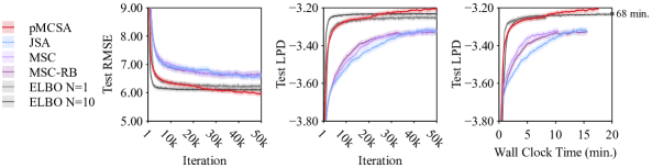
(b)

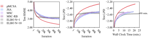
(c)

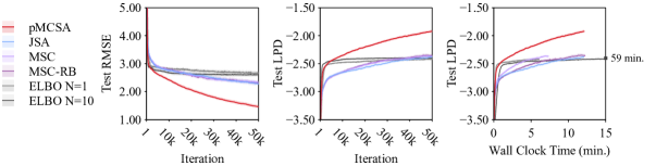
(d)

Figure 4: Test root-mean-square error (RMSE) and test log predictive density (LPD) on Bayesian neural network regression. The grey squares ($\blacksquare$) mark the performance of ELBO $N=10$ at the wall clock time shown next to it. The error bands show the 95% bootstrap confidence intervals obtained from 20 independent 90% train-test splits.

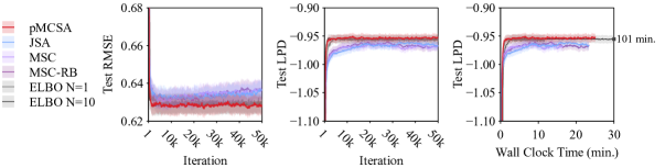
(a)

(b)

(c)

(d)

Figure 5: (continued) Test root-mean-square error (RMSE) and test log predictive density (LPD) on Bayesian neural network regression. The grey squares ($\blacksquare$) mark the performance of ELBO $N=10$ at the wall clock time shown next to it. The error bands show the 95% bootstrap confidence intervals obtained from 20 independent 90% train-test splits.

Figure 6: Distribution of the variational posterior mean of the BNN weights. The density was estimated with a Gaussian kernel and the bandwidth was selected with Silverman’s rule

E.2 Robust Gaussian Process Regression

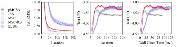
(a)

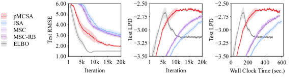
(b)

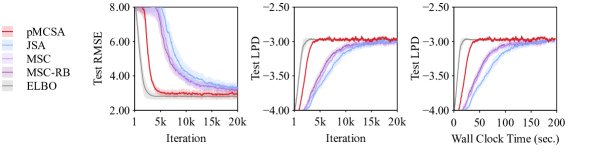
(c)

Figure 7: Test root-mean-square error (RMSE) and test log predictive density (LPD) on robust Gaussian process regression. The error bands shows the 95% bootstrap confidence interval obtained from 20 repetitions.

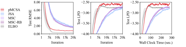
(a)

(b)

(c)

(d)

Figure 8: (continued) Test root-mean-square error (RMSE) and test log predictive density (LPD) on robust Gaussian process regression. The error bands show the 95% bootstrap confidence intervals obtained from 20 independent 90% train-test splits.