Learning Domain Adaptive Object Detection with Probabilistic Teacher

Abstract

Self-training for unsupervised domain adaptive object detection is a challenging task, of which the performance depends heavily on the quality of pseudo boxes. Despite the promising results, prior works have largely overlooked the uncertainty of pseudo boxes during self-training. In this paper, we present a simple yet effective framework, termed as Probabilistic Teacher (PT), which aims to capture the uncertainty of unlabeled target data from a gradually evolving teacher and guides the learning of a student in a mutually beneficial manner. Specifically, we propose to leverage the uncertainty-guided consistency training to promote classification adaptation and localization adaptation, rather than filtering pseudo boxes via an elaborate confidence threshold. In addition, we conduct anchor adaptation in parallel with localization adaptation, since anchor can be regarded as a learnable parameter. Together with this framework, we also present a novel Entropy Focal Loss (EFL) to further facilitate the uncertainty-guided self-training. Equipped with EFL, PT outperforms all previous baselines by a large margin and achieve new state-of-the-arts.

Code available at https://github.com/hikvision-research/ProbabilisticTeacher

1 Introduction

Convolutional neural networks have shown remarkable performance for object detection when trained on large-scale and high-quality annotated data. However, when deployed to unseen data, the detector dramatically degrades due to domain shifts such as weather changes, light conditions variations, or image corruptions (Michaelis et al., 2019). To remedy this issue, unsupervised domain adaptive object detection (UDA-OD) methods have been proposed (Chen et al., 2018; Saito et al., 2019; He & Zhang, 2019; Bousmalis et al., 2017; Hsu et al., 2020; Kim et al., 2019; Deng et al., 2021; R. et al., 2021; Li et al., 2020a), whose goal is to transfer pre-trained models from a labeled source domain to an unlabeled target domain with different data distribution. Recently, UDA-OD methods have witnessed a strong demands in real-world scenarios such as automatic driving and edge AI, where domain shifts are common and collecting high-quality annotated target data is expensive.

Figure 1: Performance comparison of adapting different models from normal to foggy weather. Our framework achieves the state-of-the-art result by simply adopting a self-training mechanism.

As shown in Fig.1, various methods have been proposed for this task, and they can be categorized as domain alignment, domain translation and self-training methods. Domain alignment aims to learn domain-invariant representation using domain classifiers and gradient reversal layers (Chen et al., 2018; Saito et al., 2019; He & Zhang, 2019). Domain translation, on the other hand, attempts to translate the labeled source data into target-like styles to drive adaptation training (Bousmalis et al., 2017; Hsu et al., 2020; Kim et al., 2019). Very recently, self-training is proposed to leverage teacher-student mutual learning to progressively improve the performance of unlabeled target data (Deng et al., 2021; R. et al., 2021). Specifically, self-training removes the necessity of extra training paradigms like adversarial training and style transfer, and has recently demonstrated promising results. Our proposed method, as will be detailed in the later sections, falls into the self-training category.

The critical component in self-training lies in the pseudo labeling. A popular solution is to filter pseudo boxes via an elaborate category confidence threshold (Deng et al., 2021; R. et al., 2021). However, there are two inherent challenges in this paradigm. Dependence challenge: the performance in this paradigm depends heavily on the selection of the threshold, while in many if not all cases, no annotated target data is available to tune the confidence threshold. Performance challenge: since only category confidence is considered while localization confidence is not, this simple solution cannot guarantee the quality of pseudo boxes (see Fig.3).

To address these issues, from the perspective of uncertainty, we present in this paper a threshold-free framework, termed as Probabilistic Teacher (PT), to apply cross-domain self-training via uncertainty-guided consistency training between the teacher and student models for both classification and localization adaptation. In our proposed framework, the existing Faster-RCNN (Ren et al., 2015) is restructured into a probabilistic one, since the existing Faster-RCNN is incapable to predict localization uncertainty. In this way, both category and localization labels can be represented as probability distributions, providing a ground for the teacher model to annotate target pseudo boxes with uncertainty.

Furthermore, another issue in prior work comes to the anchor. As a scene-sensitive parameter, anchor shapes have to be manually tweaked to improve accuracy when applying anchor-based detector to a specific object detection dataset. In the existing works, source and target domains usually share the same anchors. However, source and target domains generally have different distributions of bounding box (bbox) sizes due to domain shifts. In this paper, we propose to carry out anchor adaptation in parallel with localization adaptation. Thus, our approach unifies classification, localization and anchor adaptations into one framework.

To further facilitate uncertainty-guided self-training, we design an Entropy Focal Loss (EFL) to drive uncertainty-guided consistency training in both classification and localization branches, encouraging the model to pay more attention to the lower-entropy pseudo boxes.

Compared with the existing self-training methods, our approach does not require filtering the target pseudo boxes using a carefully fine-tuned confidence threshold. This makes our model particularly suitable for the UDA-OD setting, where no annotated target data is available for the filtering threshold tuning. Of particular importance, our PT approach can be seamlessly and effortlessly extended to source-free UDA-OD setting (privacy-critical scenario), where only unlabeled target data is involved into self-training for the purpose of privacy protection, achieving remarkable improvements compared with previous approaches.

What is worth highlighting that we draw several interesting yet novel findings via extensive ablation studies: 1) Strong data augmentation is an implicit intra-domain alignment method to bridge the intra-domain gap between the true labels and false labels in target domain. 2) Data augmentation plays a much more important role in self-training approaches than domain alignment counterparts. 3) Merely adopting localization adaptation alone can still improve the adaptation performance against “source only” remarkably.

We summarize the takeaways as well as contributions as:

• We propose a threshold-free framework to explore cross-domain object detection via an uncertainty-driven self-training paradigm. It firstly unifies classification, localization as well as anchor adaptations into one framework.

• We design an EFL loss for PT framework to further facilitate uncertainty-guided cross-domain self-training.

• We draw several interesting yet novel experimental findings, which can inspire the future works in UDA-OD.

• Our framework achieves the new state-of-the-art results on multiple source-based / free UDA-OD benchmarks, and surpasses previous approaches by a large margin.

Figure 2: Illustration of the proposed Probabilistic Teacher. Unlabeled target data with weak augmentation are fed into the teacher model to generate pseudo boxes, which contain classification and localization probability distributions. Both labeled source data and pseudo-labeled target data with sequent sharpening operation are used to train the student model via uncertainty-guided consistency training with strong data augmentation. Also, anchor adaptation is conducted in parallel with localization adaptation. To promote PT framework, Entropy Focal Loss (EFL) is proposed to further facilitate the cross-domain self-training.

Figure 3: Box variance $\sigma^{2}$ is better than foreground score to measure the localization accuracy of bboxes (IoU with ground-truth bboxes). Results on the Foggy Cityscapes are presented.

2 Related Works

Unsupervised Domain Adaptive Object Detection Several approaches have been proposed for UDA-OD, which can be categorized into domain alignment, domain translation and self-training methods. These methods have been introduced briefly in the section above. We discuss the last one more detailedly since our work is built on self-training. As mentioned above, the most critical component in self-training is to exploit pseudo boxes. To obtain more accurate pseudo boxes, Unbiased Mean Teacher (Deng et al., 2021) translates the target domain into a source-like one to generate pseudo boxes. In contrast, SimROD (R. et al., 2021) introduces a teacher model with a larger capacity to generate pseudo boxes. However, these existing works try to generate more accurate pseudo boxes using different techniques while the pseudo boxes are inevitable to be noisy. To address this problem, we propose an uncertainty-guided framework to deal with noisy pseudo boxes dynamically during cross-domain self-training.

Self Training for Object Detection Self-training methods have been explored in many previous works for semi-supervised object detection (Li et al., 2020b; Sohn et al., 2020; Liu et al., 2021; Xu et al., 2021; Chen et al., 2022; Yu et al., 2022; Yang et al., 2020b, a; Ren et al., 2022), in which pseudo boxes of unlabeled data are filtered to train the detectors using a carefully fine-tuned category confidence threshold. STAC (Sohn et al., 2020) is proposed to pre-train a detector using a small amount of labeled data and then generate pseudo boxes on unlabeled data to fine-tune the pre-trained detector. However, the pseudo boxes are generated only once and fixed throughout the rest of the training progress. Unbiased Teacher (Liu et al., 2021) attempts to update the pseudo boxes via a mean teacher mechanism, while the box regression is only performed on the labeled data. Soft Teacher (Xu et al., 2021) is proposed to use a box jitter method to measure the localization accuracy to filter the pseudo boxes. LabelMatch (Chen et al., 2022) exploits the Label Distribution Consistency assumption between labeled and unlabeled data to update the confidence threshold for pseudo labeling. It is reasonable to search for an appropriate confidence threshold using an annotated validation set for semi-supervised detection. However, no annotated target data is available for the filtering threshold tuning during UDA-OD, which inspires us to exploit the uncertainty of pseudo boxes rather than filtering the pseudo boxes via an elaborate confidence threshold.

3 Preliminary

Faster-RCNN, a benchmark detector for UDA-OD task, decouples object detection into a cross-entropy-based classification branch and a $\mathcal{L}$1-based bbox regression branch. In the classification branch, the predicted probability distribution over label space is natural to capture the classification uncertainty, while the Dirac delta modeling for bbox regression makes it incapable to obtain the localization uncertainty. To remedy this, in this section, we augment the existing Faster-RCNN detector into a probabilistic one, dubbed as Probabilistic Faster-RCNN, where both category and localization labels are represented as probability distributions.

Concretely, each coordinate ($t_{x}$, $t_{y}$, $t_{w}$, and $t_{h}$) of a bbox can be modeled as a single Gaussian model (Choi et al., 2019). Let coordinate $t$ be an univariate Gaussian distributed random variable parameterized by mean $\mu$ and variance $\sigma^{2}$: $t\sim\mathcal{N}\left(\mu,\sigma^{2}\right)$. Note that $\sigma^{2}$ is constrained as a value between zero and one with a sigmoid function. In this way, bbox regression loss can be implemented by a cross-entropy function between the ground-truth distribution $t^{GT}$ (Dirac delta one) and the predicted one $t$ (Gaussian one):

$$\mathcal{L}_{bbox} =\frac{1}{N_{bbox}}\sum_{i}\mathbb{I}_{fg}(t_{i})\mathcal{H}(t_{i}^{GT},t_{i})$$ (1)

$$\overset{\bigstar}{=}-\frac{1}{N_{bbox}}\sum_{i}\mathbb{I}_{fg}(t_{i})\log(\mathcal{N}(t_{i}^{GT};\mu_{i},\sigma_{i}^{2}))$$

where $\mathcal{H}(\cdot,\cdot)$ denotes the standard cross-entropy function. $t_{i}^{GT}$ is the ground-truth bbox coordinate associated with the $i_{th}$ predicted bbox $t_{i}$. $N_{bbox}$ is the number of anchors or proposals. $\mathbb{I}_{fg}(\cdot)$ is a sign function to indicate whether the predicted bbox is matched to an anchor or proposal. $\mu_{i}$ and ${\sigma_{i}}^{2}$ are the predicted coordinate mean and variance. $\mathcal{N}(t_{i}^{GT};\mu_{i},\sigma_{i}^{2})$ denotes the probability of $t_{i}^{GT}$ in the Gaussian distribution. As shown in Fig.3, ${\sigma_{i}}^{2}$ is better than foreground score to measure the localization accuracy. The detailed proof of step $\bigstar$ can be found in the appendix C.1.

With the probabilistic modeling for bbox regression, Probabilistic Faster-RCNN is able to capture the uncertainty of both classification and localization for each prediction. The overall training objective can be reformulated as:

$$\mathcal{L}_{S}=\mathcal{L}_{cls}^{RPN}+\mathcal{L}_{cls}^{ROI}+\mathcal{L}_{bbox}^{RPN}+\mathcal{L}_{bbox}^{ROI}$$ (2)

where all the four terms are cross-entropy losses, and equally weighted following the original Faster-RCNN. With the favor of Probabilistic Faster-RCNN, the proposed method, Probabilistic Teacher, is presented in the next section.

4 Probabilistic Teacher

4.1 Overview

We depict the overview of Probabilistic Teacher in Fig.2. Probabilistic Teacher contains two training steps, Pretraining and Mutual learning. 1) Pretraining. We train the detector using the labeled source data to initialize the detector, and then duplicate the trained weights to both the teacher and student models. 2) Mutual learning (Section 4.2). The main idea of Probabilistic Teacher is to capture the uncertainty of unlabeled target data from a gradually evolving probabilistic teacher and guides the learning of a student in a mutually beneficial manner. To achieve this, based on Probabilistic Faster-RCNN, Probabilistic Teacher delivers the weakly-augmented images from target domain to the teacher model to obtain pseudo boxes, and notably, category and location of each pseudo box are in the form of general distribution over label space and four Gaussian distributions, respectively. These pseudo boxes are then used to train the student via Uncertainty-Guided Consistency Training for both classification and localization branches. The student transfers its learned knowledge to the teacher via exponential moving average (EMA). In this way, both models can evolve jointly and continuously to improve performance.

4.2 Mutual Learning

4.2.1 Uncertainty-Guided Consistency Training

The student model is optimized on the labeled source data and the unlabeled target data with pseudo boxes generated from the teacher model. The training objective is written as:

$$\mathcal{L}_{total}=\mathcal{L}_{S}+\lambda_{T}\mathcal{L}_{T}$$ (3)

where $\mathcal{L}_{S}$ is a supervised loss on labeled source data which is identical to Eqn.2. $\mathcal{L}_{T}$ is a self-supervised loss on unlabeled target data, which imposes the uncertainty-guided consistency between the teacher and student models. $\lambda_{T}$ is the loss weight for target domain, and is set to 1 by default.

To optimize the second term, target data with weak augmentation is fed into the teacher model to generate pseudo boxes, which contains classification probability distributions $p^{PL}$ and bbox coordinate probability distributions $t^{PL}$. Both distributions are sharpened to guide the student training. Specifically, $\mathcal{L}_{T}$ consists of four training losses, including two classification losses and two bbox regression losses in RPN and ROIhead:

$$\mathcal{L}_{T}=\mathcal{L}_{T-cls}^{RPN}+\mathcal{L}_{T-cls}^{ROI}+\mathcal{L}_{T-box}^{RPN}+\mathcal{L}_{T-box}^{ROI}$$ (4)

The first two terms can be formulated as:

$$\mathcal{L}_{T-cls}^{RPN}=\frac{1}{N_{cls}^{RPN}}\sum_{i}\mathcal{H}(\mathcal{M}(\mathcal{S}_{cls}(p_{i}^{PL},\tau_{cls})),p_{i}^{RPN})$$ (5)

$$\mathcal{L}_{T-cls}^{ROI}=\frac{1}{N_{cls}^{ROI}}\sum_{i}\mathcal{H}(\mathcal{S}_{cls}(p_{i}^{PL},\tau_{cls}),p_{i}^{ROI})$$

where $p_{i}^{PL}$ is the $i_{th}$ classification probability distribution predicted by the teacher. $p_{i}^{RPN}$ and $p_{i}^{ROI}$ are the $i_{th}$ classification probability distribution in RPN and ROIhead predicted by the student. $\mathcal{S}_{cls}(\cdot,\tau_{cls})$ is a sharpening function where $\tau_{cls}$ is a temperature factor, which will be introduced later. $\mathcal{M}(\cdot)$ is a merging operation to sum up all foreground category probabilities to achieve the foreground/background probability distribution to guide RPN training. $N_{cls}^{RPN}$ and $N_{cls}^{ROI}$ are the batch size in RPN and ROIhead respectively.

The last two terms can be unified into a general form:

$$\mathcal{L}_{T-box}=\frac{1}{N_{bbox}}\sum_{i}\mathbb{I}_{fg}(t_{i})\mathcal{H}(\mathcal{S}_{bbox}(t_{i}^{PL},\tau_{bbox}),t_{i})$$ (6)

where $t_{i}^{PL}$ is the $i_{th}$ bbox coordinate probability distribution predicted by the teacher (Note that both terms are predicted in ROIhead). $t_{i}$ is the bbox coordinate probability distribution predicted by the student in RPN or ROIhead and associated with $t_{i}^{PL}$. $\mathcal{S}_{bbox}(\cdot,\tau_{bbox})$ is a sharpening function for bbox regression and $\tau_{bbox}$ is a temperature factor.

Figure 4: Intra-domain gap in the “Cityscapes to Foggy Cityscapes” adaptation task. True positives (TPs, in green color) and false negatives (FNs, in gold color) predicted by the “source only” model on the target domain. “h” and “w” represent the height and width of the predicted bounding boxes, respectively.

4.2.2 Sharpening Functions

Sharpening functions encourage the predictions to be sharp and low-entropy.

• For classification branch, $\mathcal{S}_{cls}(\cdot,\tau_{cls})$ is defined as a SoftMax function with temperature $\tau_{cls}$.

  $$\mathcal{S}_{cls}(\cdot,\tau_{cls})=SoftMax(\cdot,\tau_{cls})$$ (7)

• For bbox regression branch, the entropy of Gaussian distribution is a function of its variance ${\sigma}^{2}$ (see the appendix C.2 for the proof). Hence, $\mathcal{S}_{bbox}(\cdot,\tau_{bbox})$ is designed as:

  $$\sigma^{2}\leftarrow\sigma^{2}*\tau_{bbox}$$ (8)

When $\tau=1$ (including $\tau_{cls}$ and $\tau_{bbox}$), sharpening function is equivalent to the original SoftMax or Gaussian function. When $\tau\rightarrow 0$ or $\tau\rightarrow+\infty$, it tends to be a Dirac delta distribution or a uniform distribution, which corresponds the most low-entropy or high-entropy case. It is set as $\tau<1$ in this work. With this specialized sharpening function for bbox regression, $\mathcal{L}_{T-bbox}$ in Eqn.6 is detailed as:

$$\mathcal{L}_{T-bbox}= \frac{1}{N_{bbox}}\sum_{i}\mathbb{I}_{fg}(t_{i})[\log(\sigma_{i})$$ (9)

$$+\frac{(\sigma_{i}^{PL})^{2}*\tau_{bbox}+(\mu_{i}^{PL}-\mu_{i})^{2}}{\sigma_{i}^{2}}]+C$$

where ($\mu_{i}^{PL}$, $\sigma_{i}^{PL}$) and ($\mu_{i}$, $\sigma_{i}$) are the $i_{th}$ mean and variance of bbox coordinates predicted by the teacher and student models, respectively. $C$ is a constant. See the appendix C.3 for the detailed proof of this step.

4.2.3 Teacher Updating

To obtain more accurate pseudo boxes, EMA is applied to gradually update the teacher model with positive feedbacks from the student model. Given the weight of the student $\theta^{S}$, the teacher $\theta^{T}$ is obtained by : $\theta^{T}=\alpha\theta^{T}+(1-\alpha)\theta^{S}$, where $\alpha$ is the EMA rate. The slowly updated teacher model is regarded as an ensemble of student models in different training timestamps.

Table 1: Results of adaptation from normal to foggy weather (C2F). “†” represents that the results are reproduced by us using the released codes, with the same strong augmentation and Probabilistic Faster-RCNN. “Source only” and “Oracle” refer to the models trained by only using labeled source data and labeled target data, respectively. “FR” represents Faster-RCNN. “0.01”, “0.02” and “ALL” in the column of “split” represent the foggy level 0.01, 0.02 and all three foggy levels, respectively. “UN” means that the foggy level used in the corresponding paper is unknown based on the paper and released code (if available).

Methods	Split	Reference	Arch.	truck	car	rider	person	train	motor	bicycle	bus	mAP
Source only	0.02	-	FR+VGG16	9.0	28.5	26.6	22.4	4.3	15.2	25.3	16.0	18.4
Source only (strong aug.)	0.02	-		10.1	37.7	33.0	26.4	6.2	17.4	30.2	24.4	23.2
Source only	ALL	-		12.1	40.4	33.4	27.9	10.1	20.7	30.9	23.2	24.8
Source only (strong aug.)	ALL	-		18.6	48.1	41.3	33.9	7.3	26.6	37.8	34.5	31.0
MTOR (Cai et al., 2019)	0.02	CVPR’19		21.9	44.0	41.4	30.6	40.2	31.7	33.2	43.4	35.1
SW (Saito et al., 2019)	0.02	CVPR’19		24.5	43.5	42.3	29.9	32.6	30.0	35.3	32.6	34.3
DM (Kim et al., 2019)	UN	CVPR’19		27.2	40.5	40.5	30.8	34.5	28.4	32.3	38.4	34.6
PDA (Hsu et al., 2020)	ALL	WACV’20		24.3	54.4	45.5	36.0	25.8	29.1	35.9	44.1	36.9
GPA (Xu et al., 2020b)	0.01	CVPR’20	FR+Resnet50	24.7	54.1	46.7	32.9	41.1	32.4	38.7	45.7	39.5
ATF (He & Zhang, 2020)	UN	ECCV’20	FR+VGG16	23.7	50.0	47.0	34.6	38.7	33.4	38.8	43.3	38.7
HTCN (Chen et al., 2020a)	0.02	CVPR’20		31.6	47.9	47.5	33.2	40.9	32.3	37.1	47.4	39.8
ICR-CCR (Xu et al., 2020a)	ALL	CVPR’20		27.2	49.2	43.8	32.9	36.4	30.3	34.6	36.4	37.4
CF (Zheng et al., 2020)	UN	CVPR’20		30.8	52.1	46.9	34.0	29.9	34.7	37.4	43.2	38.6
iFAN (Zhuang et al., 2020)	UN	AAAI’20		27.9	48.5	40.0	32.6	31.7	22.8	33.0	45.5	35.3
SFOD (Li et al., 2020a)	ALL	AAAI’21		25.5	44.5	40.7	33.2	22.2	28.4	34.1	39.0	33.5
MeGA (VS et al., 2021)	UN	CVPR’21		25.4	52.4	49.0	37.7	46.9	34.5	39.0	49.2	41.8
UMT (Deng et al., 2021)	0.02	CVPR’21		34.1	48.6	46.7	33.0	46.8	30.4	37.3	56.5	41.7
SW †(Saito et al., 2019)	ALL	CVPR’19		28.7	51.0	46.3	34.2	24.0	33.8	37.1	44.9	37.5
ICR-CCR †(Xu et al., 2020a)	ALL	CVPR’20		29.7	50.4	47.2	33.6	35.1	34.6	37.9	50.0	39.8
PT	0.02	Ours		30.7	59.7	48.8	40.2	30.6	35.4	44.5	51.8	42.7
PT	ALL	Ours		33.4	63.4	52.4	43.2	37.8	41.3	48.7	56.6	47.1
Oracle	0.02	-		33.1	59.1	47.3	39.5	42.9	38.1	40.8	47.3	43.5
Oracle	ALL	-		32.6	61.6	49.1	41.2	49.0	37.9	42.4	56.6	46.3

4.2.4 Anchor Adaptation

In the existing works, source and target domains usually share the same anchors. However, source and target domains generally have different distributions of bbox sizes due to domain shifts. It is intuitive to adapt the anchors automatically during self-training. Specifically, anchors have been proven to be learnable parameters (Zhong et al., 2020). We propose to adapt the anchor shapes slowly during teacher-student mutual learning in an EMA mechanism to match the distribution of bboxes in target domain. The overall optimization objective is:

$$\min_{\theta^{S}}\{{\mathcal{L}_{S}+\min_{\mathrm{\{(w_{k},h_{k})\}_{k=1}^{A}}}{\lambda_{T}\mathcal{L}_{T}}}\}$$ (10)

where $\{(w_{k},h_{k})\}_{k=1}^{A}$ is the anchor shapes, and A is the number of anchors.

4.3 Entropy Focal Loss

Although PT has exploited the noisy pseudo boxes in a step-by-step manner that the predictions are encouraged to be low-entropy gradually, the existing noisy pseudo boxes may inevitably harm the performance. Since the proposed framework can obtain the uncertainty of each bbox (category plus four coordinates), it is reasonable to apply these uncertainty information to improve performance. Based on this intuitive thought, we use the entropy of category and location to describe the uncertainty of each bbox, and introduce an entropy focal loss to further facilitate uncertainty-guided consistency training for both classification and localization branches. Entropy focal loss for classification and regression branches can be unified into a general form:

$$\mathcal{H}_{EFL}(\cdot,\cdot)=\left(1-\mathcal{E}/\mathcal{E}_{norm}\right)^{\lambda}\mathcal{H}(\cdot,\cdot)$$ (11)

where $\lambda$ is a hyperparameter, $\mathcal{E}$ is the prediction entropy from the teacher, and $\mathcal{E}_{norm}$ is the norm term. $\mathcal{E}_{norm}$ is set as the maximal value of the entropy. Theoretically, $\mathcal{E}_{norm}$ equals $\log(n+1)$ for classification and equals $\frac{1}{2}\log(2\pi)+\frac{1}{2}$ for localization (see the Appendix C.2 and C.4 for the detailed proof), where $n$ is the number of foreground classes.

With the obtained uncertainty for the category and each coordinate of pseudo boxes, Entropy Focal Loss encourages the model to pay more attention to less noisy category predictions in classification branch and more accurate coordinate individuals in regression branch.

5 Strong Augmentation for UDA-OD

5.1 Intra-Domain Gap

We visualize the true positives (TPs) and false negatives (FNs) predicted by the “source only” model on the target domain in Fig.4. We obeserve that the smaller, severelier blurred and occluded objects tend to have a poorer adaptation performance and vice verse. We dub this phenomenon as intra-domain gap. As observed in qualitative results in Fig.5, intra-domain gap are commonly-exist in UDA-OD community. However, unlike inter-domain gap has been addressed in many previous works, intra-domain gap, one of the bottlenecks restricting the performance of UDA-OD, in contrast, has been neglected.

5.2 Intra-Domain Alignment via Strong Augmentation

Our findings about the issue of intra-domain gap in UDA-OD leads us to introduce strong data augmentation into our framework. Concretely, since large-scale, distinct objects usually attain high confidence score during pseudo labeling, we transform these to mimic those small scale, blurred and occluded ones via strong data augmentation (random resizing, guassian blur, color jitter and etc.). In this way, these transformed objects with low-entropy pseudo labels will guide the model to pay more attention to small scale, blurred and occluded ones. From this perspective, strong data augmentation is actually an implicit intra-domain alignment method to bridge the intra-domain gap.

6 Experiments

6.1 Experimental Settings

Datasets. To validate our approach, we conduct extensive experiments on multiple benchmarks with four different types of domain shifts, including 1) C2F: adaptation from normal to foggy weather, 2) C2B: adaptation from small to large-scale dataset, 3) K2C: adaptation across cameras, 4) S2C: adaptation from synthetic to real images. Five public datasets are used in our experiments.

• Cityscapes (C) (Cordts et al., 2016) contains 2,975 training images and 500 validation images with pixel-level annotations. The annotations are transformed into bounding boxes for the following experiments.

• Foggy Cityscapes (F) (Sakaridis et al., 2018) is a synthetic dataset rendered from Cityscapes with three levels of foggy weather (0.005, 0.01, 0.02), which correspond to the visibility ranges of 600, 300 and 150 meters.

• BDD100k (B) (Yu et al., 2018) is a large-scale dataset consisting of 100k images. The subset of images labeled as daytime, including 36,728 training and 5,258 validation images, are used for the following experiments.

• Sim10k (S) (Johnson-Roberson et al., 2016) consists of 10k images rendered by a gaming engine. In Sim10k, bounding boxes of 58,701 cars are provided in the 10,000 training images. All images are used in the experiments.

• KITTI (K) (Geiger et al., 2012) is collected by an autonomous driving platform, including 14999 images and 80256 bounding boxes. Only the train set is used here.

Network Architecture. We take Faster-RCNN as the base detector following (Chen et al., 2018), where VGG16 (Simonyan & Zisserman, 2014) pre-trained on ImageNet (Krizhevsky et al., 2012) is used as its backbone. We rescale all images by setting the shorter side of each image to 600 while keeping the aspect ratios unchanged. Our implementation is built upon Detectron2 (Wu et al., 2019).

Table 2: Results of adaptation from small to large-scale dataset (C2B). Please refer to Table 1 for notations illustration.

Methods	Reference	Arch.	mAP
Source only	-	FR+VGG16	20.6
Source only (strong aug.)	-		26.9
ICR-CCR (Xu et al., 2020a)	CVPR’20		26.9
SFOD (Li et al., 2020a)	AAAI’21		29.0
SW †(Saito et al., 2019)	CVPR’19		27.6
ICR-CCR †(Xu et al., 2020a)	CVPR’20		29.5
PT	Ours		34.9
Oracle	-		51.7

Table 3: Results of adaptation across cameras (K2C). Please refer to Table 1 for notations illustration.

Methods	Reference	Arch.	AP of car
Source only	-	FR+VGG16	40.3
Source only (strong aug.)	-		46.4
ATF (He & Zhang, 2020)	ECCV’20		42.1
GPA (Xu et al., 2020b)	CVPR’20	FR+Resnet50	47.9
SFOD (Li et al., 2020a)	AAAI’21	FR+VGG16	44.6
MeGA (VS et al., 2021)	CVPR’21		43.0
SimROD (R. et al., 2021)	ICCV’21	YOLOv5	47.5
SW †(Saito et al., 2019)	CVPR’19	FR+VGG16	47.1
ICR-CCR †(Xu et al., 2020a)	CVPR’20		47.6
PT	Ours		60.2
Oracle	-		66.4

Strong Augmentation. We use the same data augmentation strategy in (Chen et al., 2020b) except RandomResizedCrop. Instead, random resizing is applied to the images. Weak augmentation refers to random horizontal-flipping. See Appendix B for more implementation details.

Optimization. We use a batch size of 16 for both source and target data on a single GPU and train for 30k iterations with a fixed learning rate of 0.016, including 4k iterations for Pretraining and 26k iterations for Multual Learning. The detector is trained by an SGD optimizer with the momentum of 0.9 and the weight decay of $10^{-4}$. The EMA rate $\alpha$ is set to 0.9996. Without careful tuning, the loss weights in this paper are all set to 1. Moreover, $\lambda$ in EFL, together with temperature $\tau_{cls}$ and $\tau_{bbox}$, are all set to 0.5 simply.

Evaluation Protocol and Comparison Baselines. Following the existing works, we evaluate our method with the standard mean average precision (mAP) at the IOU threshold of 0.5. In our experiments, we observe that both strong augmentation and Probabilistic Faster-RCNN contribute to the baseline performance. For a fair comparison, first, we reproduce two existing works SW (Saito et al., 2019) and ICR-CCR (Xu et al., 2020a), using released codes with strong augmentation and Probabilistic Faster-RCNN. Second, we conduct extensive ablation studies in Section 6.6.

Table 4: Results of adaptation from synthetic to real images (S2C). Please refer to Table 1 for notations illustration.

Methods	Reference	Arch.	AP of car
Source only	-	FR+VGG16	35.5
Source only (strong aug.)	-		44.5
SW (Saito et al., 2019)	CVPR’19		40.7
ATF (He & Zhang, 2020)	ECCV’20		42.8
HTCN (Chen et al., 2020a)	CVPR’20		42.5
iFAN (Zhuang et al., 2020)	AAAI’20		46.9
CF (Zheng et al., 2020)	CVPR’20		43.8
GPA (Xu et al., 2020b)	CVPR’20	FR+Resnet50	47.6
SFOD (Li et al., 2020a)	AAAI’21	FR+VGG16	42.9
MeGA (VS et al., 2021)	CVPR’21		44.8
UMT (Deng et al., 2021)	CVPR’21		43.1
SimROD (R. et al., 2021)	ICCV’21	YOLOv5	52.1
SW †(Saito et al., 2019)	CVPR’19	FR+VGG16	45.4
ICR-CCR †(Xu et al., 2020a)	CVPR’20		46.1
PT	Ours		55.1
Oracle	-		66.4

6.2 C2F: Adaptation from Normal to Foggy Weather

In real-world scenarios, such as automatic driving, object detectors may be applied under different weather conditions. To study adaptation from normal to foggy weather, we use labeled Cityscapes and unlabeled Foggy Cityscapes (train set) for cross-domain self-training, and then report the evaluation results on the validation set of Foggy Cityscapes.

Notably, after investigating the existing works and the released code (if available), we find that the dataset spilts of Foggy Cityscapes they used differ from each other. We validate our approach on two most commonly used splits, level 0.02 and all three levels for a fair comparison. We use all three levels in the following ablation studies. Table 1 shows that our method achieves a new SOTA result in both splits. Notably, strong augmentation improves “source only” of level 0.02 and all three levels by +4.8 and +6.2 mAP, respectively. Compared with other approaches, our method achieves 42.7 mAP for level 0.02 and 47.1 mAP for all three levels, outperforming the best baseline MeGA (VS et al., 2021) by a large margin (+0.9/+5.3).

Table 5: The effectiveness of anchor adaptation (AA) and EFL.

Methods	C2F	C2B	K2C	S2C
PT	47.1	34.9	60.2	55.1
PT w/o AA	46.5 (-0.6)	34.4 (-0.5)	59.0 (-1.2)	54.3 (-0.8)
PT w/o AA & EFL	45.4 (-1.7)	32.9 (-2.0)	58.6 (-1.6)	54.1 (-1.0)

Table 6: Results of extension to source-free setting.

Methods	Source data	Reference	mAP
			C2F	C2B	K2C	S2C
SFOD	✗	AAAI’21	33.5	29.0	44.6	42.9
PT	✗	Ours	38.7	28.1	59.6	54.1
PT	✓	Ours	47.1	34.9	60.2	55.1
Oracle	-	-	46.3	51.7	66.4	66.4

6.3 C2B: Adaptation from Small to Large-Scale Dataset

Currently, collecting and labeling large amounts of image data with different scene layout can be extremely costly, e.g., automatic driving from one city to another. To study the effectiveness of our method for adaptation to a large-scale dataset with different scene layout, we use Cityscapes as a smaller source domain dataset, BDD100k containing distinct attributes as a large unlabeled target domain dataset. Following ICR-CCR (Xu et al., 2020a) and SFOD (Li et al., 2020a), we report the results on seven common categories on both datasets. Table 2 shows the results of this experiment, where our method outperforms all the baselines. Our method achieves 34.9 mAP, a large margin (+5.4) compared to ICR-CCR (Xu et al., 2020a).

6.4 K2C: Adaptation across Cameras

Different camera setups (e.g., angle, resolution, quality, and type) widely exist in the real world, which causes domain shift. In this experiment, we study the adaptation between two real datasets. The KITTI and Cityscapes datasets are used as source and target domains, respectively. The results are provided in Table 3. Our proposed method improves upon the best method GPA (Xu et al., 2020b) by +12.7 mAP. Notably, our method also outperforms the very recent work SimROD, which takes YOLOv5 (Jocher et al., 2021) as the base detector and relies on a large-scale teacher model.

6.5 S2C: Adaptation from Synthetic to Real Images

Synthetic images offer an alternative to alleviate the data collection and annotation problems. However, there is a distribution gap between synthetic data and real data. To adapt the synthetic scenes to the real one, we utilize the entire Sim10k dataset as source data and the training set of Cityscapes as target data. Since only the car category is annotated in both domains, we report the AP of car in the test set of Cityscapes. As provided in Table 4, our method outperforms existing approaches by a large margin, which improves over the current best method by +3.0 mAP.

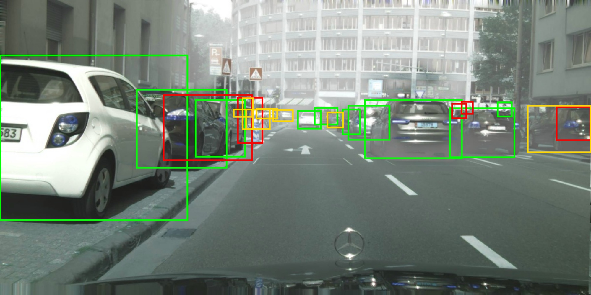
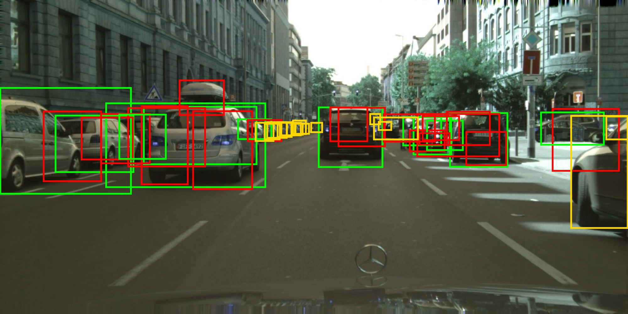
(a) Source only

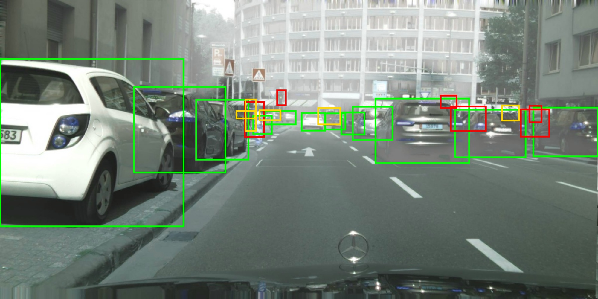
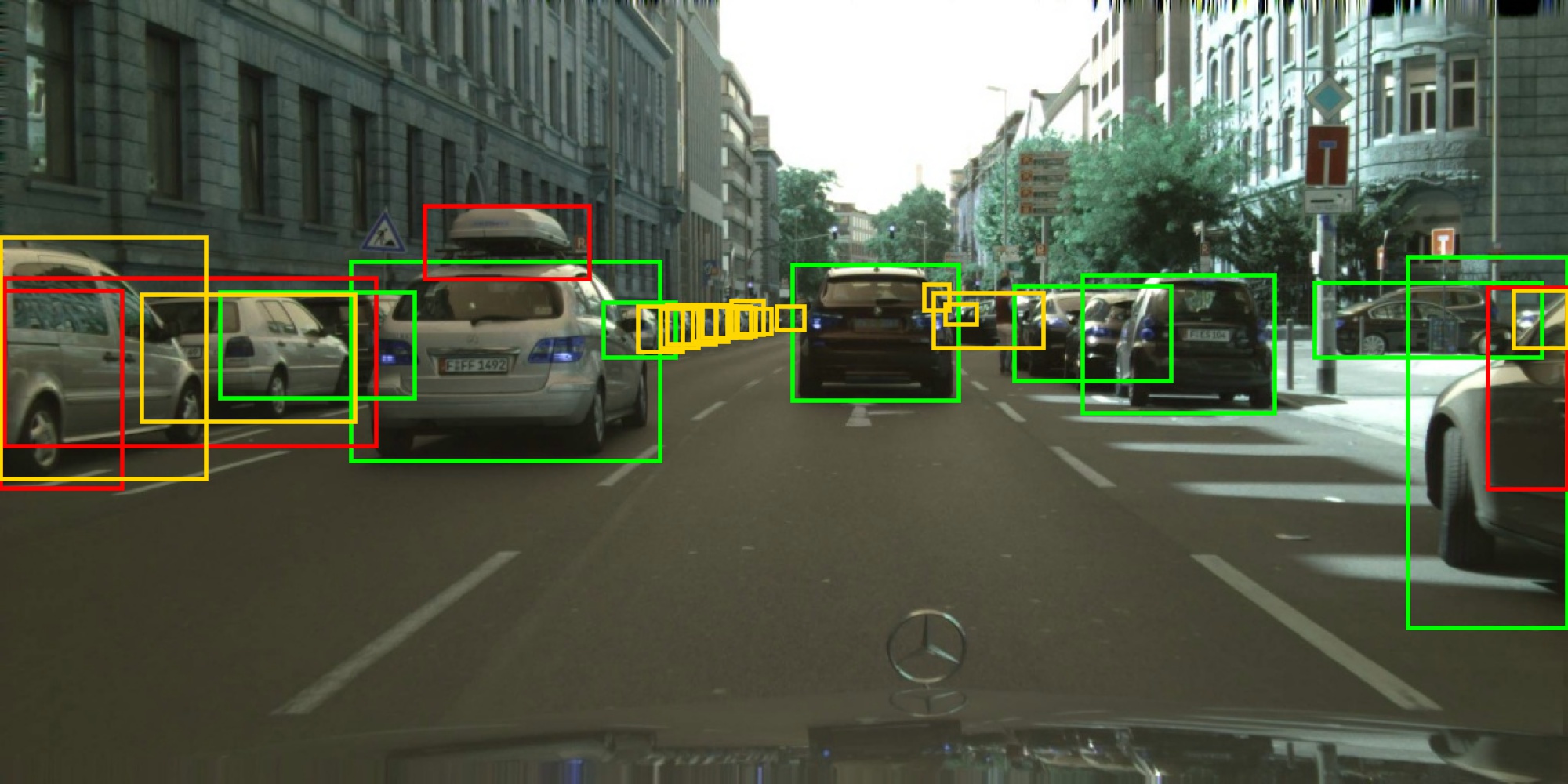
(b) SW

(c) PT

Figure 5: Qualitative results on the target domain of C2F (top row) and K2C (bottom row). Green, red and gold boxes denote true positives, false positives and false negatives, respectively.

6.6 Ablation Studies

Table 7: Performance under different data augmentations. ”F”, ”C”, ”G”, ”B”, ”S” and ”R” denote Random Horizontal Flipping, Colorjitter, Grayscale, Gaussian Blur, Solarization and Resize, respectively.

F	C	G	B	S	R	mAP
✓						34.4
✓	✓					37.6
✓	✓	✓				38.5
✓	✓	✓	✓			40.1
✓	✓	✓	✓	✓		42.5
✓	✓	✓	✓	✓	✓	47.1

Augmentation. Table 7 shows that augmentation is crucial for learning domain adaptive object detection. Specifically, the stronger the augmentation is, the better the performance is. As claimed in Section 5, we argue that one serious issue neglected by previous works in UDA-OD is the intra-domain gap. Strong augmentation can be viewed as an implicit intra-domain alignment method to bridge the intra-domain gap between true labels and false labels in target domain, and that is why we introduce strong augmentation into our method. Considering this, as shown in Table 1-4, we have re-implemented two state-of-the-art domain alignment approaches with strong augmentation for fair comparisons, from which we find that strong data augmentation obtains much more performance enhancement in self-training paradigm than domain alignment counterparts.

Anchor adaptation and EFL. Table 5 shows the effectiveness of anchor adaptation (AA) and EFL, and it can be observed that both contribute to the improvement on all four different types of domain shifts. The effectiveness of AA indicates the necessity of addressing the objects size (scale) shifts in UDA-OD task, while the effectiveness of EFL supports the claim that the obtained entropy uncertainty of pseudo boxes can be used to further boost the performance.

Extension to source-free setting. Only with the self-supervised loss on target domain, PT can be seamlessly and effortlessly extended to source-free UDA-OD (privacy-critical scenario) (Li et al., 2020a; Chen et al., 2021a, b; Huang et al., 2022), where only unlabeled target data is involved for the purpose of privacy protection. Table 6 shows that PT achieves substantial improvements, showing its robustness and scalability. Of particular interest, the performances of PT w/o and w/ source data in both K2C and S2C are almost comparable, while in C2F and C2B, there are still a large gap, which we remain for a future research.

Table 8: The effect of Probabilistic Faster-RCNN. “Source only” results are presented.

Models	C2F	C2B	K2C	S2C
Vanilla Faster-RCNN	30.2	26.3	45.9	44.1
Probabilistic Faster-RCNN	31.0	26.9	46.4	44.5

Table 9: “Thres.” and “$\tau$” are short for threshold and ($\tau_{cls}$, $\tau_{bbox}$).

Thres.	0.5	0.6	0.7	0.8	0.9	mean$\uparrow$	std$\downarrow$
mAP	35.9	33.9	49.0	56.1	56.5	46.2	9.6
$\tau$	(0.25, 0.5)	(0.75, 0.5)	(0.5, 0.5)	(0.5, 0.25)	(0.5, 0.75)	mean$\uparrow$	std$\downarrow$
mAP	59.3	58.9	60.2	57.6	59.9	59.2	0.9

The effect of uncertainty. We perform the self-training of Faster-RCNN with different confidence thresholds under the same mean-teacher framework. As shown in Fig.6, we observe the same phenomenon as (Li et al., 2020a) that the performance varies widely across different thresholds. The proposed PT, in contrast, a threshold-free approach, achieves remarkable SOTA results compared to Faster-RCNN with different confidence thresholds.

The effect of probabilistic modeling. PT is derived from Probabilistic Faster-RCNN to unify classification and localization adaptations into one framework. The “source only” results of both vanilla and Probabilistic one are presented in Table 8, showing that the improvement brought by probabilistic modeling is trivial and limited. For a fair comparison, we have re-implemented two state-of-the-art approaches with Probabilistic Faster-RCNN in Table 1-4.

The entropy of pseudo labels. Fig.7 visualizes the mean entropy of the pseudo boxes on Foggy Cityscapes dataset as the training goes on in Mutual Learning stage. We can observe that both the category and box entropy show a similar trend that they increase in a small step initially and then keep decreasing stably. It indicates that the categories of the pseudo boxes on the target domain are getting more confident, and the locations of the pseudo boxes are getting more accurate during cross-domain self-training.

Figure 6: Performance curve of K2C, using PT and vanilla Faster-RCNN with different confidence thresholds.

Analysis of hyper-parameters. Fig.8 provides the ablation studies of several hyper-parameters, including $\lambda$ in EFL, temperature parameters $\tau_{cls}$ and $\tau_{bbox}$. Experiments with only classification (w/o $\mathcal{L}_{T-bbox}^{RPN}+\mathcal{L}_{T-bbox}^{ROI}$, the left sub-figure of Fig.8) or localization (w/o $\mathcal{L}_{T-cls}^{RPN}+\mathcal{L}_{T-cls}^{ROI}$, the right sub-figure of Fig.8) adaptation under different hyper-parameters combinations are conducted. The results show that even adapting classification or localization alone can still significantly boost performance against the “source only”. For $\lambda$ in EFL, the adaptation performance goes up as $\lambda$ increases in classification branches while it is opposite in localization branches. For $\tau_{cls}$ and $\tau_{bbox}$, a too large or too small temperature will hurt the performance. In our paper, we set them without careful tuning (all are set to 0.5).

Furthermore, to provide a more systematic analysis about the robustness of PT w.r.t the temperature, we re-conduct the ablation study of ($\tau_{cls}$, $\tau_{bbox}$) in K2C adaptation setting, as well as a comparison with threshold-based setting. As shown in Table 9, PT is actually more superior (see “mean”) and robust (see “std”) than the threshold-based method.

Qualitative visualization. As shown in Fig.5, we present qualitative results of C2F and K2C to demonstrate the improvement brought by PT. The visualizations show that PT can significantly ease the intra-domain gap, i.e. reducing the false-positives and increasing the true-positives. Consequently, the performance is improved by a large margin. See Appendix A for more experimental results.

Figure 7: The mean entropy of the pseudo boxes. Box entropy denotes the averaged location entropy across four coordinates.

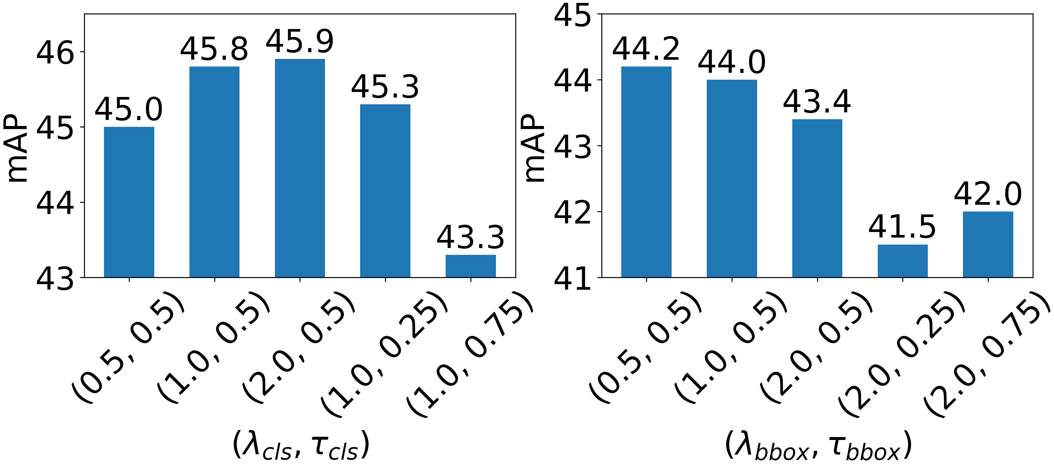
Figure 8: Ablation studies of C2F on hyper parameter $\lambda$ in EFL and $\tau$ in sharpening functions.

7 Conclusions

In this paper, we propose a simple yet effective framework, Probabilistic Teacher, to study the utilization of uncertainty during cross-domain self-training. Equipped with the novel Entropy Focal Loss, this framework can achieve new state-of-the-art results on multiple source-based / free UDA-OD benchmarks. We look forward that our method may bring inspirations to other weakly-supervised object detection tasks, such as noisy-label-supervised object detection.

Appendix A More Experimental Results

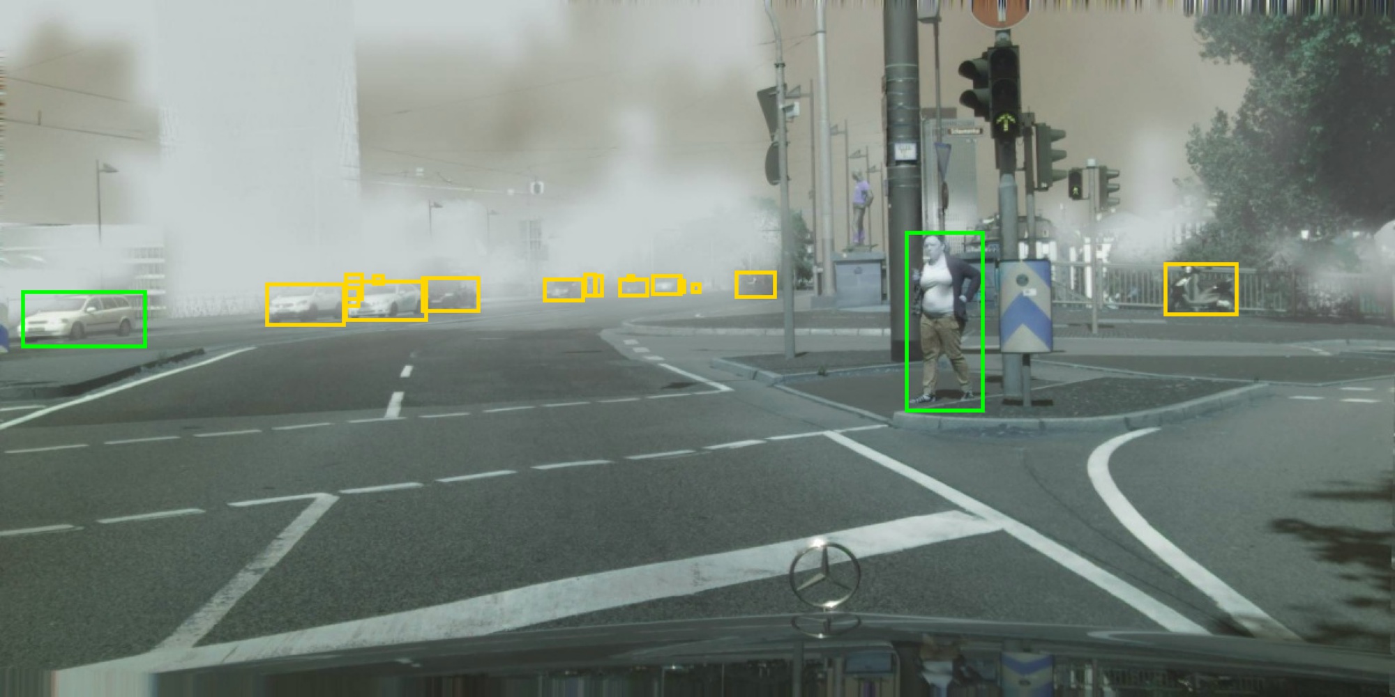
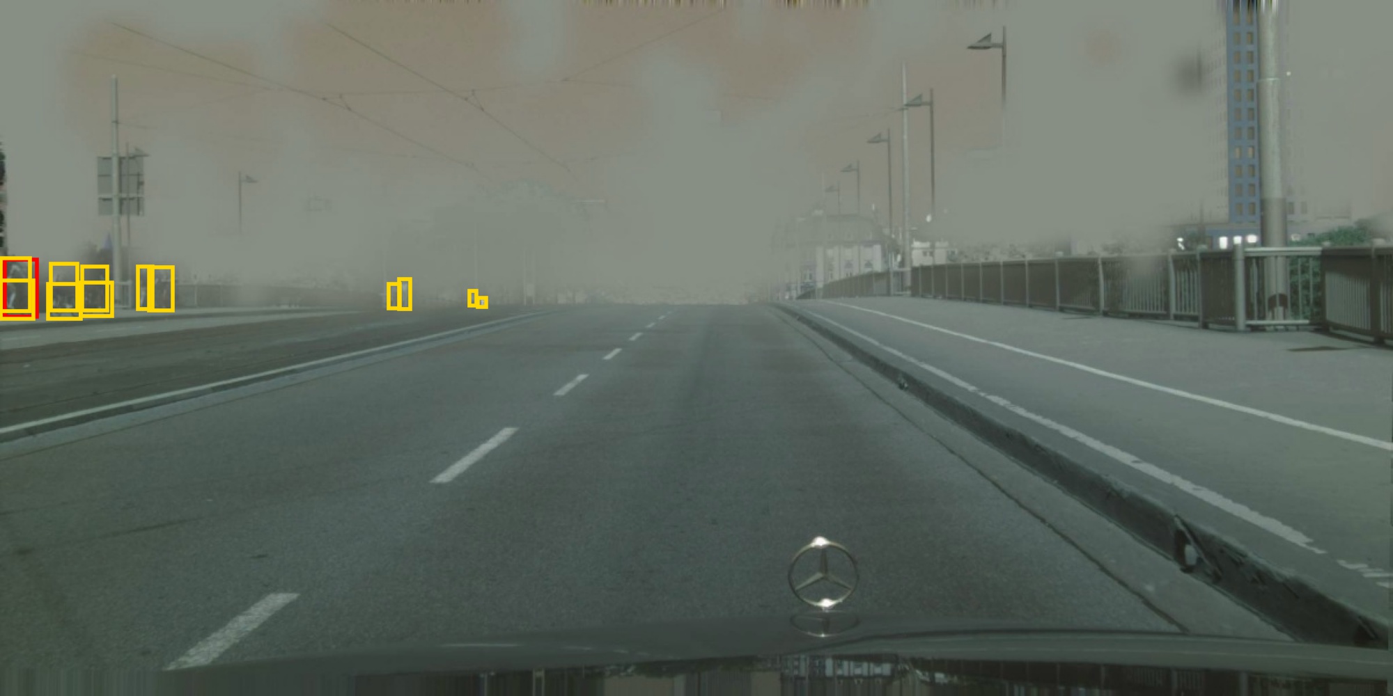
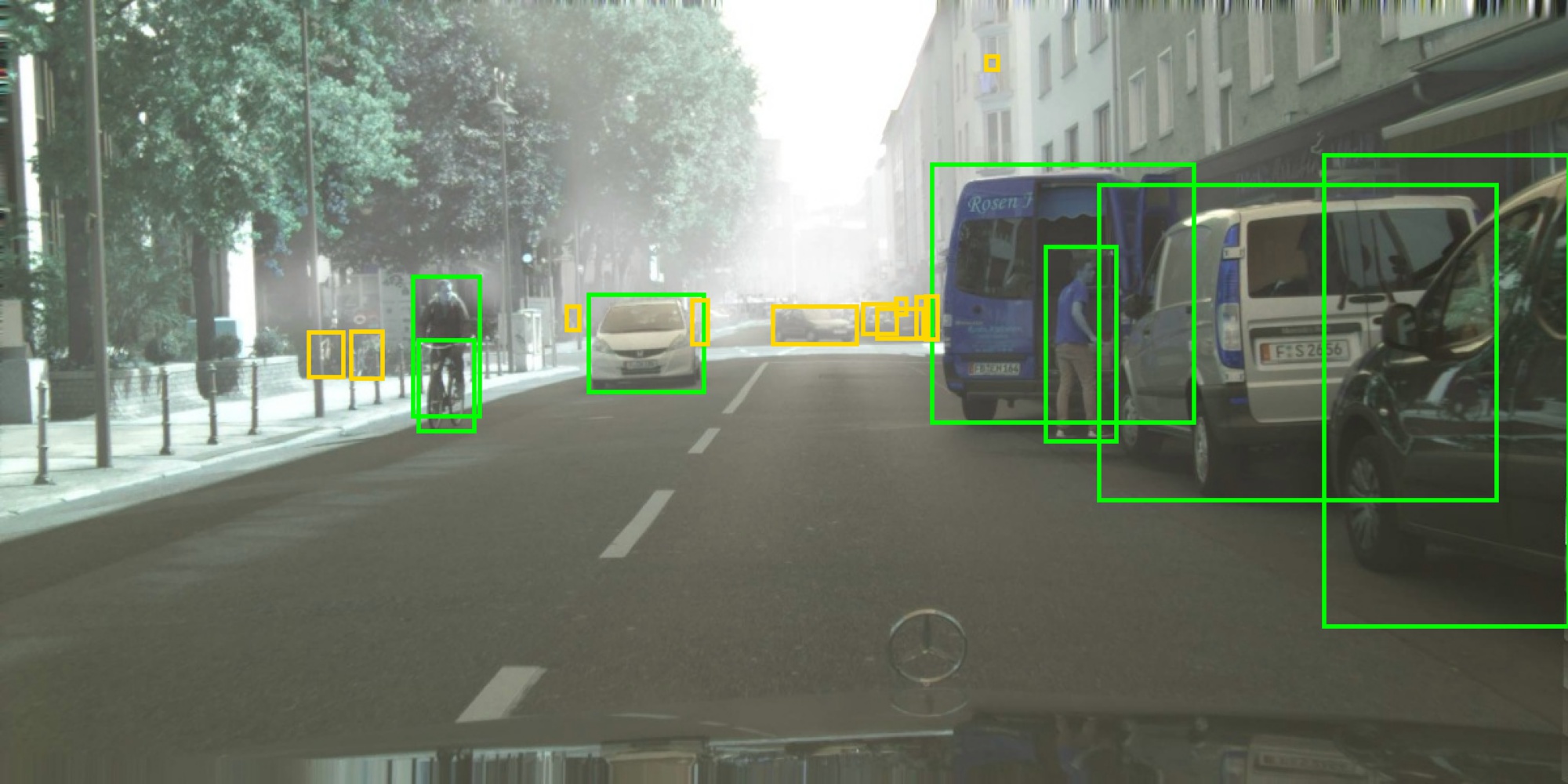
(a) Source only

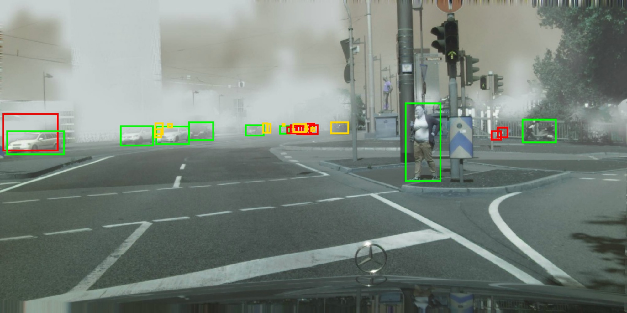
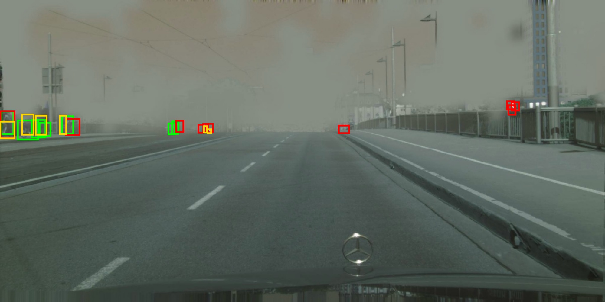
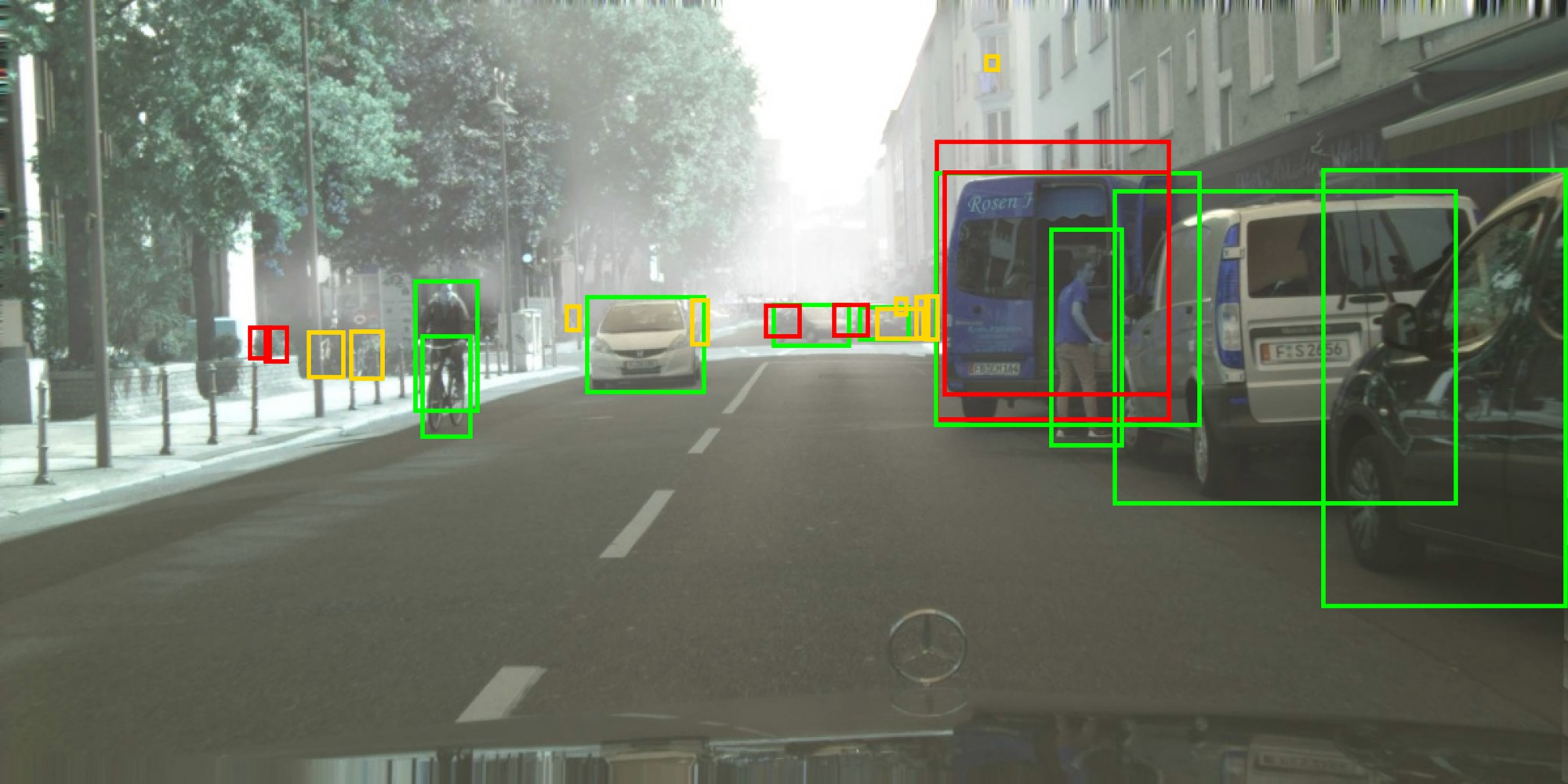
(b) SW

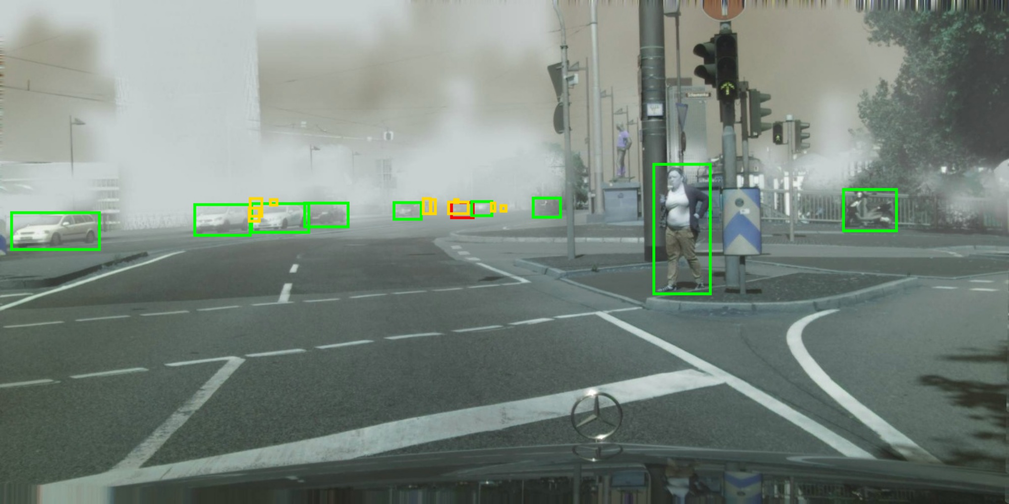
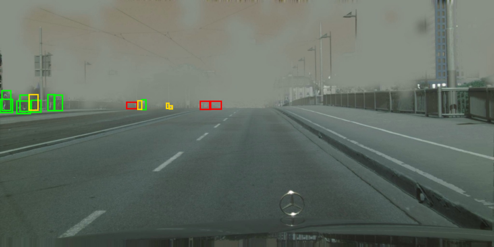
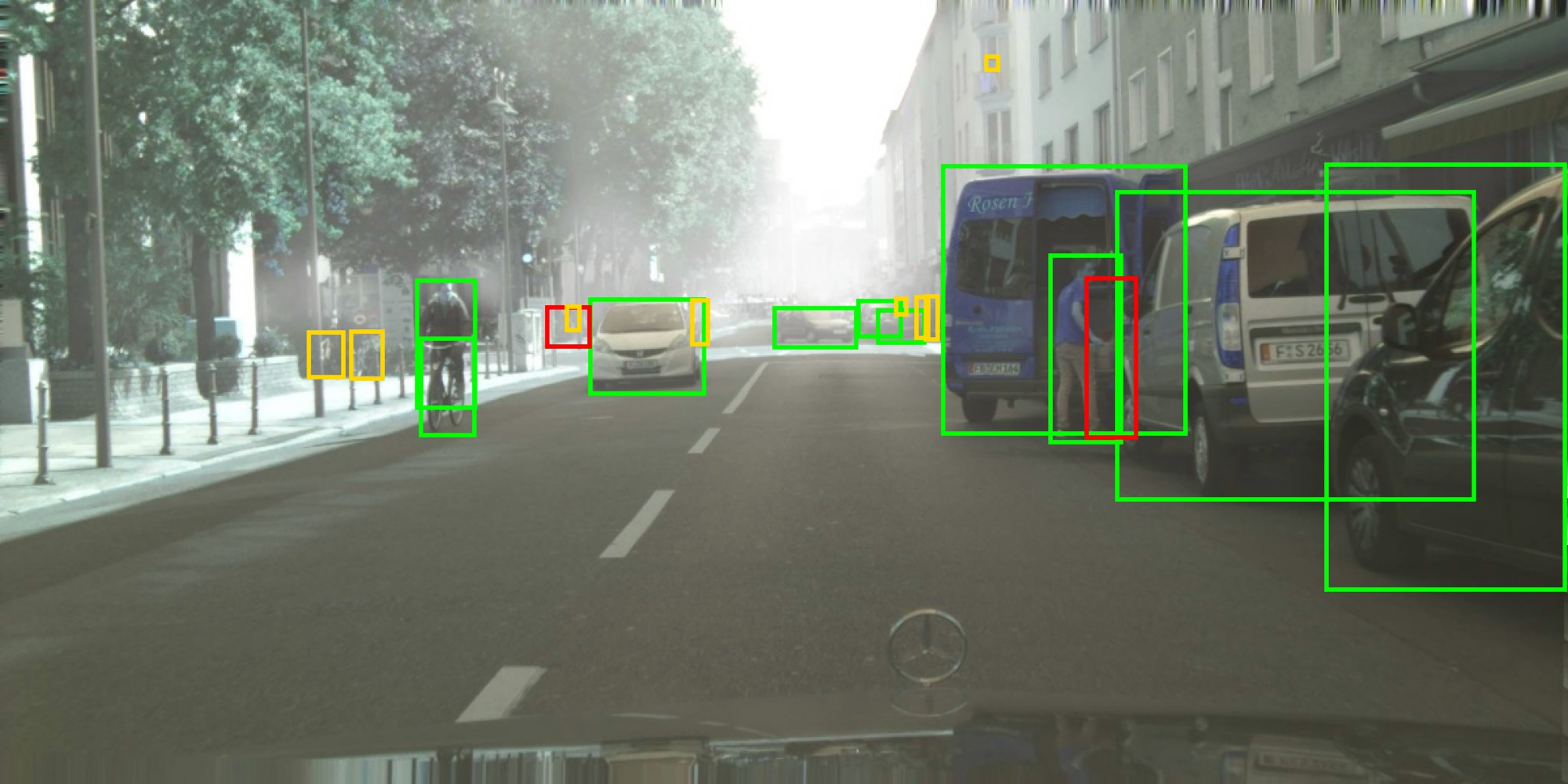
(c) PT

Figure 9: More results on the target domain of C2F. Green, red and gold boxes denote true positives, false positives and false negatives, respectively.

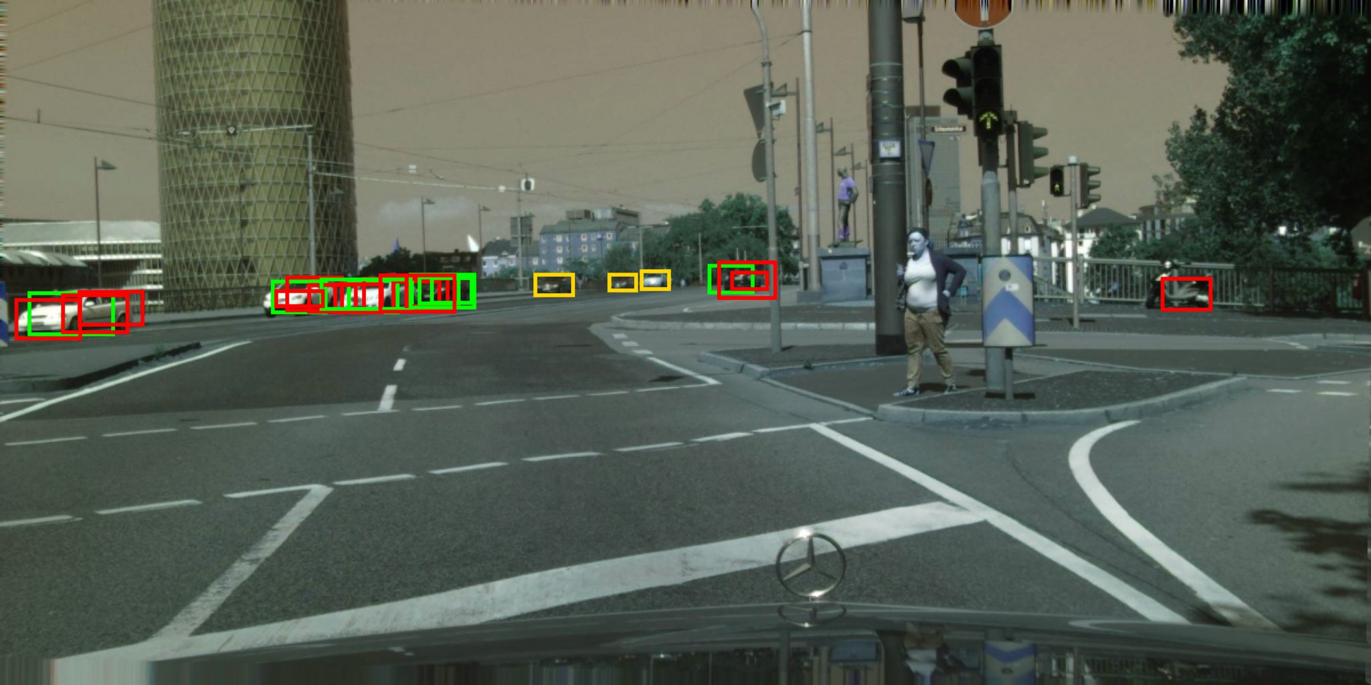
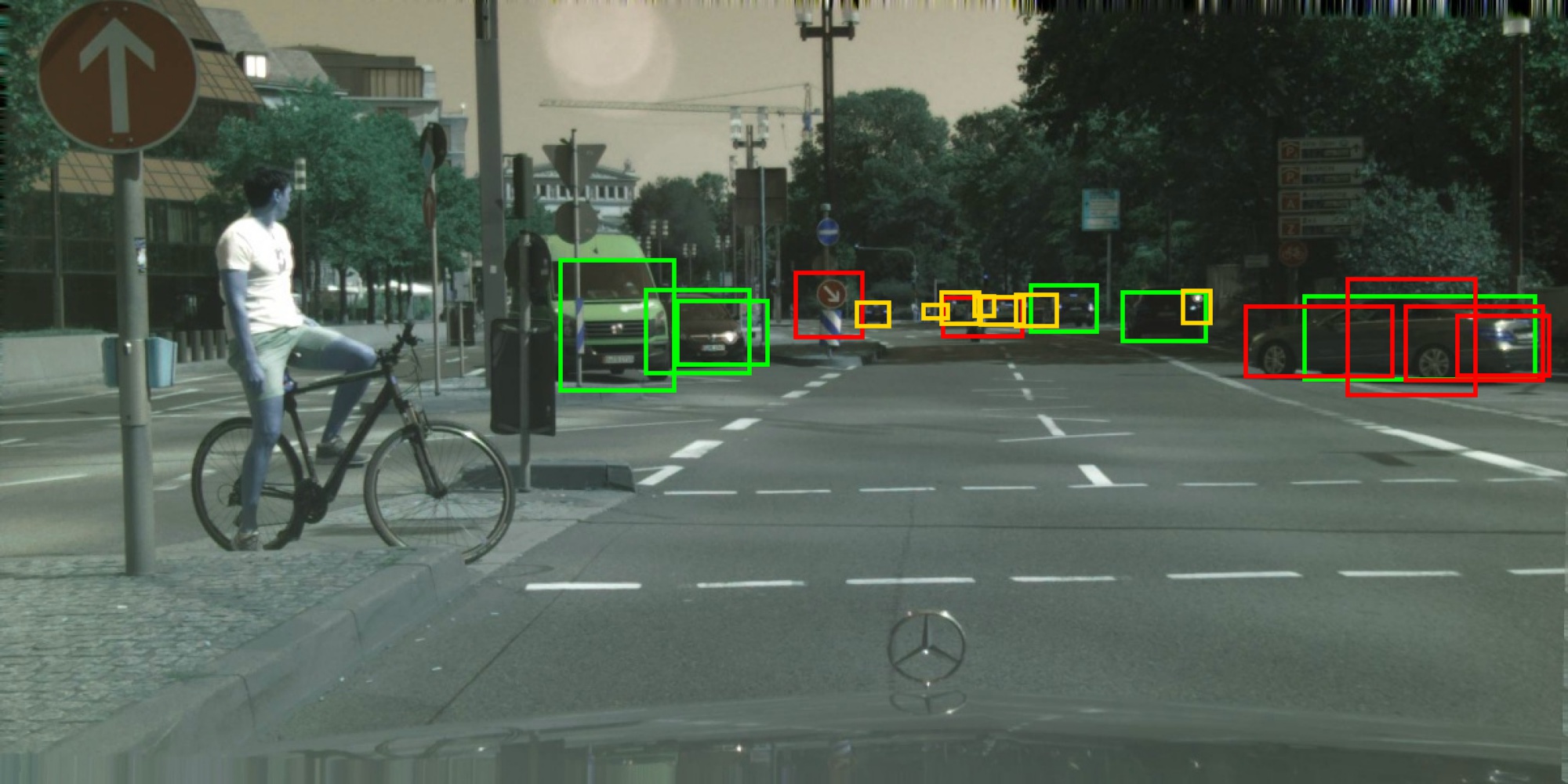
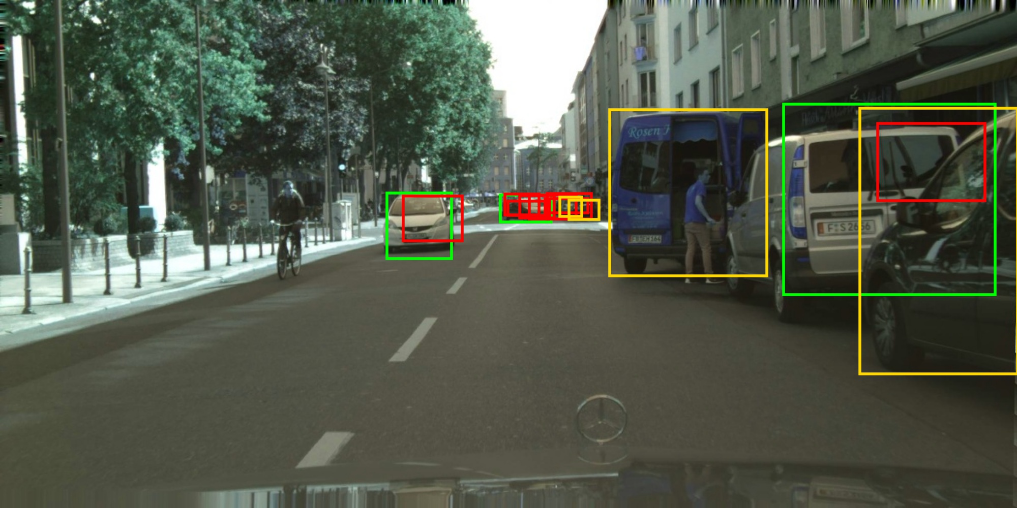
(a) Source only

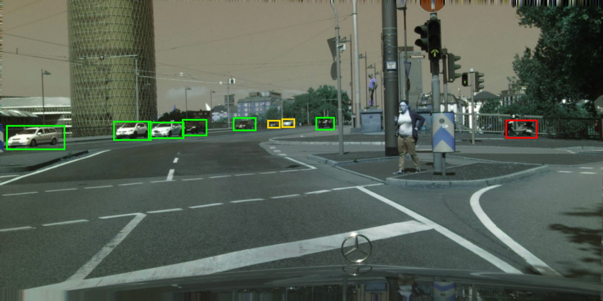
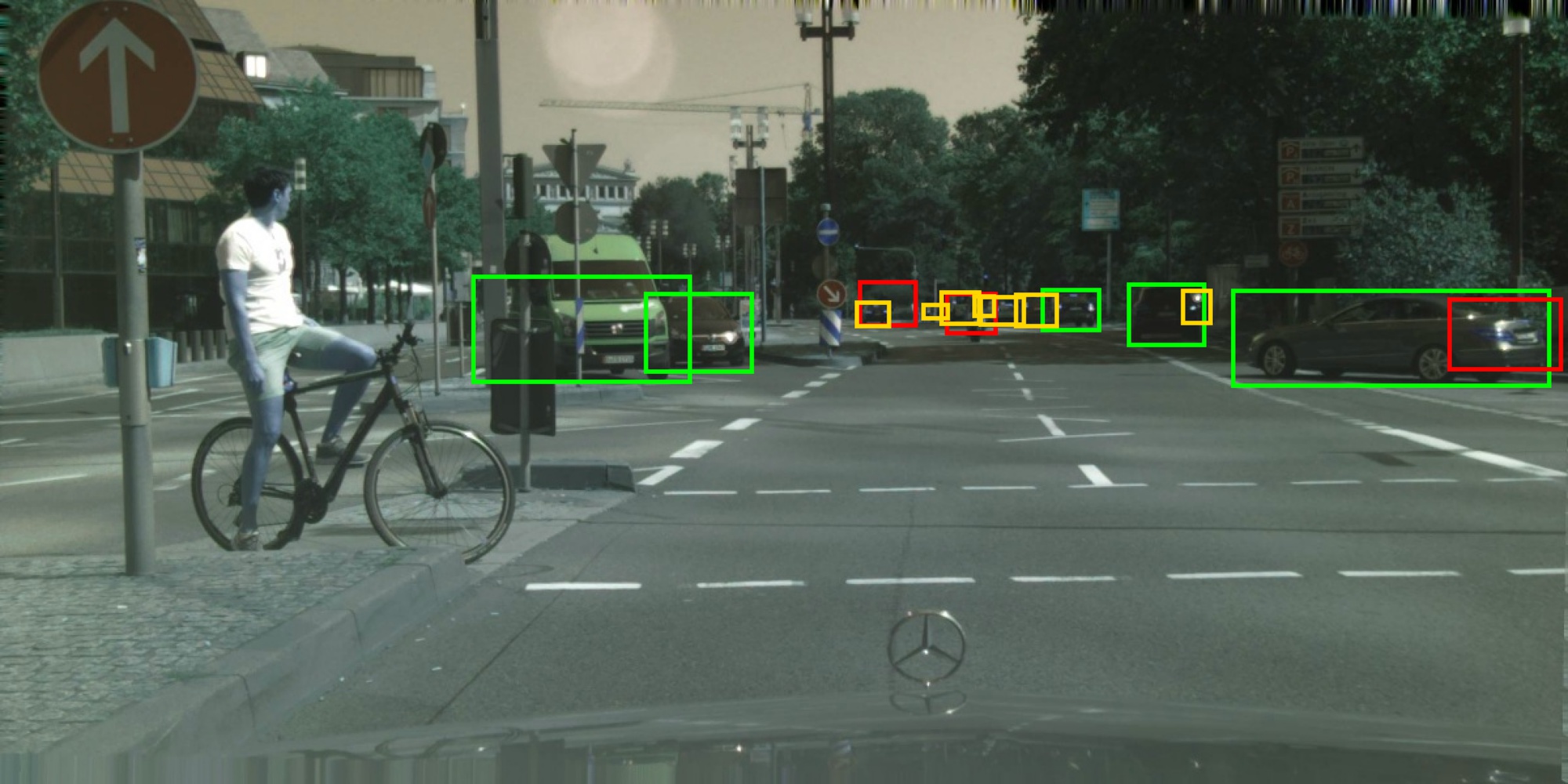
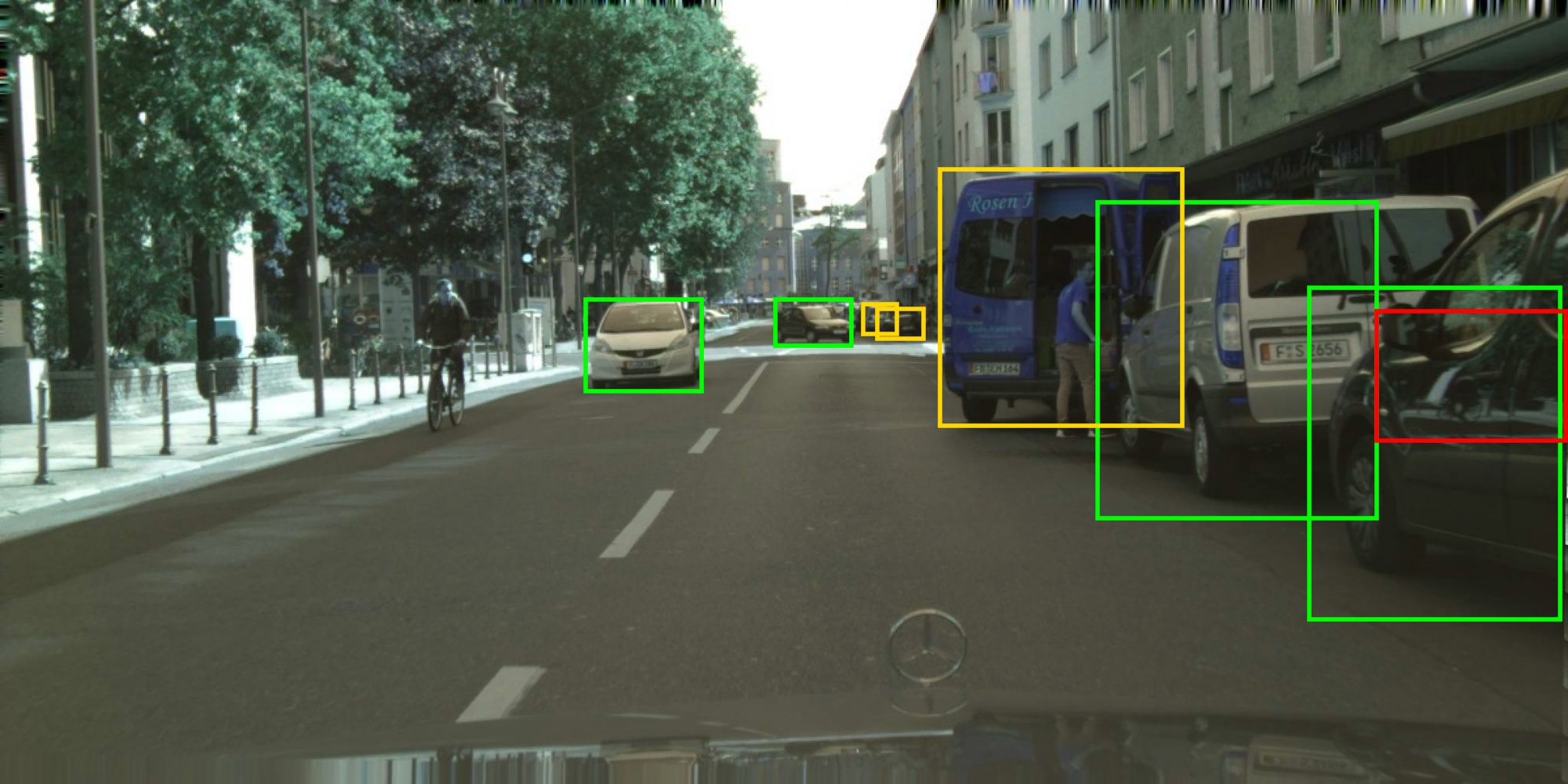
(b) SW

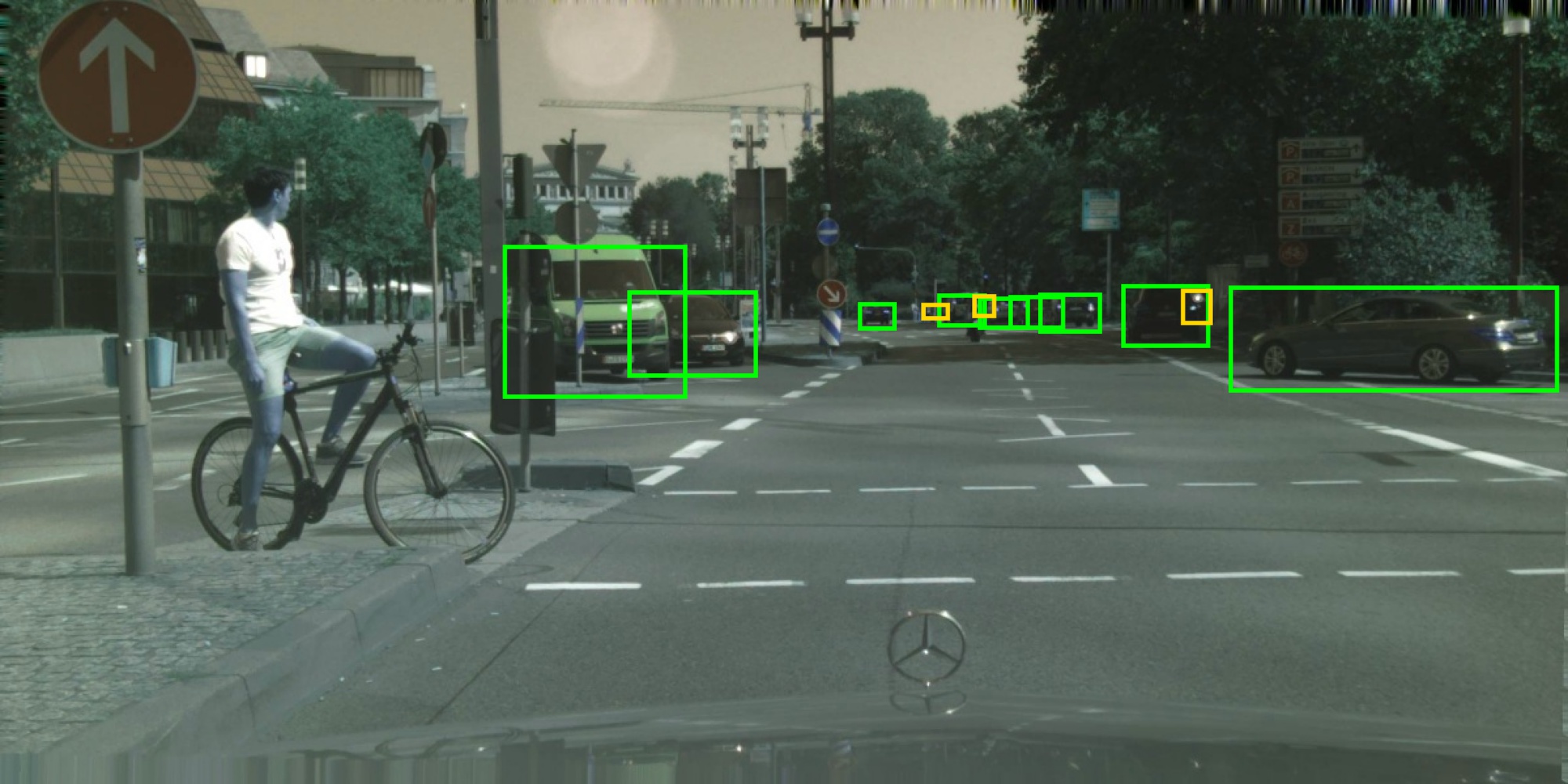
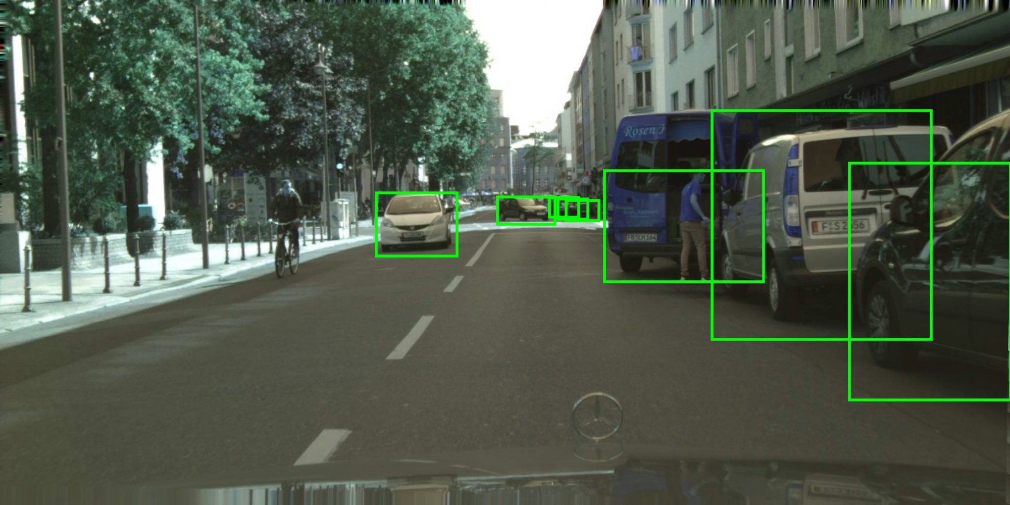
(c) PT

Figure 10: More results on the target domain of K2C. Green, red and gold boxes denote true positives, false positives and false negatives, respectively.

A.1 More Qualitative Visualization

In Fig.9 and Fig.10, we present more qualitative detection results of two adaptation tasks to demonstrate the improvement brought by our PT framework.

Appendix B More Implementation Details

B.1 Anchor adaptation

In our implementation, the initial anchor shapes simply follow the original Faster-RCNN, i.e., 3 sizes (128, 256, 512), 3 aspects ratios (0.5, 1, 2) at each output sliding window position. In this way, only additional $9\times 2$ learnable parameters are required during anchor adaptation.

B.2 Data Augmentation Details

In this paper, we use the same set of strong augmentation in SimCLR (Chen et al., 2020b) except the RandomResizedCrop. We perform random horizontal-flipping, followed by color jitter and grayscale conversion. And then Gaussian blur and solarization are applied randomly to the images. Moreover, simple random resizing is applied to the images, which are then padded to the original size. Specifically, random resizing in our implementation is to zoom out the images randomly within (0.5, 1) while keeping the aspect ratios unchanged. The code for augmentation above using torchvision is as follows:

⬇

1from torchvision import transforms

2augmentation = []

3augmentation.append(transforms.RandomApply([HorizontalFlipping()], p=0.5))

4augmentation.append(transforms.RandomApply([transforms.ColorJitter(0.4, 0.4, 0.4, 0.1)], p=0.8))

5augmentation.append(transforms.RandomGrayscale(p=0.2))

6augmentation.append(transforms.RandomApply([GaussianBlur([0.1, 2.0])], p=0.5))

7augmentation.append(transforms.RandomApply([Solarize(threshold=0.5)], p=0.2))

8augmentation.append(transforms.RandomApply([RandomResizing(0.5, 1.0)], p=1.0))

B.3 Pseudo-Code of PT

Algorithm 1 summarizes the pseudo-code of PT. PT consists of two training stages, including Pretraining and Mutual Learning. In the Pretraining stage, we train the detector using the labeled source data to initialize the detector, and then duplicate the trained weights to both the teacher and student models. In the Mutual Learning stage, the generated pseudo boxes on the unlabeled target data and the labeled source data are used to train the student via uncertainty-guided consistency training for both classification and localization branches. The student then transfers its learned knowledge to the teacher via EMA. In this way, both models can evolve jointly and continuously to improve performance.

Algorithm 1 Probabilistic Teacher

0:  Source domain $D_{S}$, Target domain $D_{T}$

1:  while Pretraining do

2:     Train source only model $\theta^{I}$ based on Eq. (3)

3:  end while

4:  $\theta^{S}\leftarrow\theta^{I}$ COMMENT# Duplicate to student model

5:  $\theta^{T}\leftarrow\theta^{I}$ COMMENT# Duplicate to teacher model

6:  while Mutual Learning do

7:     Calculate $\mathcal{L}_{S}$ based on Eq. (3)

8:     $p^{PL},t^{PL}\leftarrow\theta^{T}(D_{T})$ COMMENT# Pseudo labeling, weak augmentation

9:     $p^{PL}\leftarrow\mathcal{S}_{cls}(p^{PL},\tau_{cls})$ COMMENT# Sharpen classification probability distributions

10:     $t^{PL}\leftarrow\mathcal{S}_{bbox}(t^{PL},\tau_{bbox})$ COMMENT# Sharpen localization probability distributions

11:     $p,t\leftarrow\theta^{S}(D_{T})$ COMMENT# Feed forward, strong augmentation

12:     Calculate EFL $\mathcal{L}_{T-cls}^{ROI}$ based on Eq. (6) and Eq. (11) COMMENT# Classification adaptation

13:     $p^{PL}\leftarrow\mathcal{M}(p^{PL})$ COMMENT# Merging operation to sum up all foreground probabilities

14:     Calculate EFL $\mathcal{L}_{T-cls}^{RPN}$ based on Eq. (6) and Eq. (11) COMMENT# Classification adaptation

15:     Calculate EFL $\mathcal{L}_{T-bbox}^{ROI}$ based on Eq. (7) and Eq. (11) COMMENT# Regression adaptation

16:     Calculate EFL $\mathcal{L}_{T-bbox}^{RPN}$ based on Eq. (7) and Eq. (11) COMMENT# Regression adaptation

17:     $\mathcal{L}_{T}=\mathcal{L}_{T-cls}^{RPN}+\mathcal{L}_{T-cls}^{ROI}+\mathcal{L}_{T-box}^{RPN}+\mathcal{L}_{T-box}^{ROI}$

18:     $\mathcal{L}_{total}=\mathcal{L}_{S}+\lambda_{T}\mathcal{L}_{T}$

19:     Train the anchor shapes via minimizing $\mathcal{L}_{T}$ COMMENT# Anchor adaptation

20:     Train student model $\theta^{S}$ via minimizing $\mathcal{L}_{total}$

21:     Update teacher model via EMA

22:  end while

Appendix C Mathematical Proofs

In this section, we provide the rigorous proofs mentioned in the main body of the paper.

C.1 The cross-entropy between a Dirac delta distribution and a univariate Gaussian distribution

Given $p(x)=\delta(x-a)$ and $q(x)=N(x;\mu,\sigma^{2})$, the cross-entropy between $p(x)$ and $q(x)$, $H(p,q)$, can be written as:

$$H(p,q) =-\int p(x)\log q(x)dx$$

$$=-\int\delta(x-a)\log(N(x;\mu,\sigma^{2}))dx$$

Expanding the $\log$ term,

$$H(p,q) =-\int\delta(x-a)\log(N(x;\mu,\sigma^{2}))dx$$

$$=\frac{1}{2}\int\delta(x-a)\left(\log(2\pi)+2\log\sigma+\left(\frac{x-\mu}{\sigma}\right)^{2}\right)dx$$

Because,

$$\delta(x-a) =0,(x\neq a)$$

$$\int\delta(x-a)dx =1$$

The cross-entropy between $p(x)$ and $q(x)$, $H(p,q)$, can be simplified as:

$$H(p,q)=\frac{1}{2}\left(\log(2\pi)+2\log\sigma+\left(\frac{a-\mu}{\sigma}\right)^{2}\right)$$

C.2 The entropy of a univariate Gaussian distribution

Let $x$ be a univariate Gaussian distributed random variable:

$$x\sim\textit{N}\left(x;\mu,\sigma^{2}\right)$$

The differential entropy of $x$, $H(x)$, can be written as:

$$H(x) =-\int p(x)\log p(x)\mathbf{d}x$$

$$=\frac{1}{2}\log\left(2\pi\sigma^{2}\right)+\frac{1}{2\sigma^{2}}\mathrm{E}\left[(x-\mu)^{2}\right]$$

The expectation of $(x-\mu)^{2}$, ${E}[($x$-\mu)^{2}]$, is equal to the variance:

$$E[(x-\mu)^{2}]=\sigma^{2}$$

Substituting this back in the earlier expression gives us the result,

$$H(x){=}\frac{1}{2}\log\left(2\pi\sigma^{2}\right)+\frac{1}{2}$$

The entropy of a univariate Gaussian distribution is only the function of its variance. The maximal value in our paper is $\frac{1}{2}\log\left(2\pi\right)+\frac{1}{2}$ since $\sigma$ is processed as a value between zero and one with a sigmoid function.

C.3 The cross-entropy between two univariate Gaussian distributions

Given $p(x)=\textit{N}\left(x;\mu_{1},\sigma_{1}^{2}\right)$ and $q(x)=\textit{N}\left(x;\mu_{2},\sigma_{2}^{2}\right)$ , the cross-entropy between $p(x)$ and $q(x)$, $H(p,q)$, can be written as,

$$H(p,q) =-\int p(x)\log q(x)dx$$

$$=-\int\textit{N}\left(x;\mu_{1},\sigma_{1}^{2}\right)\log(\textit{N}\left(x;\mu_{2},\sigma_{2}^{2}\right))dx$$

Expanding the $\log$ term,

$$H(p,q) =-\int\textit{N}\left(x;\mu_{1},\sigma_{1}^{2}\right)\log(\textit{N}\left(x;\mu_{2},\sigma_{2}^{2}\right))dx$$

$$=\frac{1}{2}\int\textit{N}\left(x;\mu_{1},\sigma_{1}^{2}\right)\left(\log(2\pi)+2\log\sigma_{2}+\left(\frac{x-\mu_{2}}{\sigma_{2}}\right)^{2}\right)dx$$

Because the integral over a PDF is always 1,

$$\int\textit{N}\left(x;\mu,\sigma^{2}\right)dx=1$$

Moving the constant outside,

$$H(p,q)=\frac{1}{2}\left(\log(2\pi)+2\log\sigma_{2}\right)+\frac{1}{2}\int\textit{N}\left((x;\mu_{2},\sigma_{2}^{2}\right)\left(\frac{x-\mu_{2}}{\sigma_{2}}\right)^{2}dx$$

Now let’s only consider the second term. Because,

$$\left(\frac{x-\mu_{2}}{\sigma_{2}}\right)^{2}=\left(\frac{x-\mu_{1}}{\sigma_{1}}\right)^{2}\frac{\sigma_{1}^{2}}{\sigma_{2}^{2}}+x\frac{2\left(\mu_{1}-\mu_{2}\right)}{\sigma_{2}^{2}}+\frac{\mu_{2}^{2}-\mu_{1}^{2}}{\sigma_{2}^{2}}$$

The second term can be expanded as,

$$\frac{1}{2}\int\textit{N}\left(x;\mu_{2},\sigma_{2}^{2}\right)\left(\frac{x-\mu_{2}}{\sigma_{2}}\right)^{2}dx =\frac{1}{2}\int\textit{N}\left(x;\mu_{2},\sigma_{2}^{2}\right)\left(\left(\frac{x-\mu_{1}}{\sigma_{1}}\right)^{2}\frac{\sigma_{1}^{2}}{\sigma_{2}^{2}}+x\frac{2\left(\mu_{1}-\mu_{2}\right)}{\sigma_{2}^{2}}+\frac{\mu_{2}^{2}-\mu_{1}^{2}}{\sigma_{2}^{2}}\right)dx$$

$$= \frac{1}{2\sigma_{2}^{2}}\int\textit{N}\left(x;\mu_{2},\sigma_{2}^{2}\right)\left(x-\mu_{1}\right)^{2}dx+\frac{\left(\mu_{1}-\mu_{2}\right)}{\sigma_{2}^{2}}\int\textit{N}\left(x;\mu_{2},\sigma_{2}^{2}\right)xdx$$

$$+\frac{1}{2}\frac{\mu_{2}^{2}-\mu_{1}^{2}}{\sigma_{2}^{2}}\int\textit{N}\left(x;\mu_{2},\sigma_{2}^{2}\right)dx$$

Because, 1) the integral over a PDF is always 1; 2) the expectation of x, E(x), is equal to the mean; 3) the expectation of $(x-\mu)^{2}$, ${E}[($x$-\mu)^{2}]$, is equal to the variance, and these are,

$$\int\textit{N}\left(x;\mu,\sigma^{2}\right)dx =1$$

$$\int xN(x;\mu,\sigma^{2})dx =\mu$$

$$\int(x-\mu)^{2}N(x;\mu,\sigma^{2})dx =\sigma^{2}$$

Therefore,

$$\frac{1}{2}\int\textit{N}\left(x;\mu_{2},\sigma_{2}^{2}\right)\left(\frac{x-\mu_{2}}{\sigma_{2}}\right)^{2}dx=\frac{1}{2}\left(\frac{\sigma_{1}^{2}}{\sigma_{2}^{2}}+\frac{2\mu_{1}\left(\mu_{1}-\mu_{2}\right)}{\sigma_{2}^{2}}+\frac{\mu_{2}^{2}-\mu_{1}^{2}}{\sigma_{2}^{2}}\right)$$

Substituting this back in the earlier expression gives us the result,

$$H(p,q) =\frac{1}{2}\left(\log(2\pi)+2\log\sigma_{2}+\frac{\sigma_{1}^{2}}{\sigma_{2}^{2}}+\frac{2\mu_{1}\left(\mu_{1}-\mu_{2}\right)}{\sigma_{2}^{2}}+\frac{\mu_{2}^{2}-\mu_{1}^{2}}{\sigma_{2}^{2}}\right)$$

$$=\log\sigma_{2}+\frac{\sigma_{1}^{2}+(\mu_{1}-\mu_{2})^{2}}{2\sigma_{2}^{2}}+C$$

where C is a constant.

C.4 Maximal value of a discrete variable’s entropy

Let $x$ be a discrete variable,

$$x\sim p(x)$$

Its entropy, $H(x)$, can be written as,

$$H(x) =-\sum p(x)\log p(x)$$

$$=E[\log\frac{1}{p(x)}]$$

This means that the entropy of $x$ is equal to the expectation of $\log\frac{1}{p(x)}$. Using the Jensen inequality,

$$E[\log\frac{1}{p(x)}]\leq\log E[\frac{1}{p(x)}]=\log n$$

where $n$ is the number of all possible events. Maximal value is attained when all possible events are equiprobable.

References

- Bousmalis et al. (2017) Bousmalis, K., Silberman, N., Dohan, D., Erhan, D., and Krishnan, D. Unsupervised pixel-level domain adaptation with generative adversarial networks. In Proceedings of the IEEE conference on computer vision and pattern recognition, pp. 3722–3731, 2017.
- Cai et al. (2019) Cai, Q., Pan, Y., Ngo, C.-W., Tian, X., Duan, L., and Yao, T. Exploring object relation in mean teacher for cross-domain detection. In Proceedings of the IEEE/CVF Conference on Computer Vision and Pattern Recognition, pp. 11457–11466, 2019.
- Chen et al. (2022) Chen, B., Chen, W., Yang, S., Xuan, Y., Song, J., Xie, D., Pu, S., Song, M., and Zhuang, Y. Label matching semi-supervised object detection. In Proceedings of the IEEE/CVF Conference on Computer Vision and Pattern Recognition, 2022.
- Chen et al. (2020a) Chen, C., Zheng, Z., Ding, X., Huang, Y., and Dou, Q. Harmonizing transferability and discriminability for adapting object detectors. In Proceedings of the IEEE/CVF Conference on Computer Vision and Pattern Recognition, pp. 8869–8878, 2020a.
- Chen et al. (2020b) Chen, T., Kornblith, S., Norouzi, M., and Hinton, G. A simple framework for contrastive learning of visual representations. In International conference on machine learning, pp. 1597–1607. PMLR, 2020b.
- Chen et al. (2021a) Chen, W., Guo, Y., Yang, S., Li, Z., Ma, Z., Chen, B., Zhao, L., Xie, D., Pu, S., and Zhuang, Y. Box re-ranking: Unsupervised false positive suppression for domain adaptive pedestrian detection. 2021a.
- Chen et al. (2021b) Chen, W., Lin, L., Yang, S., Xie, D., Pu, S., Zhuang, Y., and Ren, W. Self-supervised noisy label learning for source-free unsupervised domain adaptation. CoRR, abs/2102.11614, 2021b. URL https://arxiv.org/abs/2102.11614.
- Chen et al. (2018) Chen, Y., Li, W., Sakaridis, C., Dai, D., and Van Gool, L. Domain adaptive faster r-cnn for object detection in the wild. In Proceedings of the IEEE conference on computer vision and pattern recognition, pp. 3339–3348, 2018.
- Choi et al. (2019) Choi, J., Chun, D., Kim, H., and Lee, H.-J. Gaussian yolov3: An accurate and fast object detector using localization uncertainty for autonomous driving. In Proceedings of the IEEE/CVF International Conference on Computer Vision, pp. 502–511, 2019.
- Cordts et al. (2016) Cordts, M., Omran, M., Ramos, S., Rehfeld, T., Enzweiler, M., Benenson, R., Franke, U., Roth, S., and Schiele, B. The cityscapes dataset for semantic urban scene understanding. In Proceedings of the IEEE conference on computer vision and pattern recognition, pp. 3213–3223, 2016.
- Deng et al. (2021) Deng, J., Li, W., Chen, Y., and Duan, L. Unbiased mean teacher for cross-domain object detection. In Proceedings of the IEEE/CVF Conference on Computer Vision and Pattern Recognition, pp. 4091–4101, 2021.
- Geiger et al. (2012) Geiger, A., Lenz, P., and Urtasun, R. Are we ready for autonomous driving? the kitti vision benchmark suite. In 2012 IEEE conference on computer vision and pattern recognition, pp. 3354–3361. IEEE, 2012.
- He & Zhang (2019) He, Z. and Zhang, L. Multi-adversarial faster-rcnn for unrestricted object detection. In Proceedings of the IEEE/CVF International Conference on Computer Vision, pp. 6668–6677, 2019.
- He & Zhang (2020) He, Z. and Zhang, L. Domain adaptive object detection via asymmetric tri-way faster-rcnn. In Computer Vision–ECCV 2020: 16th European Conference, Glasgow, UK, August 23–28, 2020, Proceedings, Part XXIV 16, pp. 309–324. Springer, 2020.
- Hsu et al. (2020) Hsu, H.-K., Yao, C.-H., Tsai, Y.-H., Hung, W.-C., Tseng, H.-Y., Singh, M., and Yang, M.-H. Progressive domain adaptation for object detection. In Proceedings of the IEEE/CVF Winter Conference on Applications of Computer Vision, pp. 749–757, 2020.
- Huang et al. (2022) Huang, J., Chen, W., Yang, S., Xie, D., Pu, S., and Zhuang, Y. Transductive clip with class-conditional contrastive learning. In ICASSP, 2022.
- Jocher et al. (2021) Jocher, G., Stoken, A., Borovec, J., NanoCode012, Chaurasia, A., TaoXie, Changyu, L., V, A., Laughing, tkianai, yxNONG, Hogan, A., lorenzomammana, AlexWang1900, Hajek, J., Diaconu, L., Marc, Kwon, Y., oleg, wanghaoyang0106, Defretin, Y., Lohia, A., ml5ah, Milanko, B., Fineran, B., Khromov, D., Yiwei, D., Doug, Durgesh, and Ingham, F. ultralytics/yolov5: v5.0 - YOLOv5-P6 1280 models, AWS, Supervise.ly and YouTube integrations, April 2021. URL https://doi.org/10.5281/zenodo.4679653.
- Johnson-Roberson et al. (2016) Johnson-Roberson, M., Barto, C., Mehta, R., Sridhar, S. N., Rosaen, K., and Vasudevan, R. Driving in the matrix: Can virtual worlds replace human-generated annotations for real world tasks? arXiv preprint arXiv:1610.01983, 2016.
- Kim et al. (2019) Kim, T., Jeong, M., Kim, S., Choi, S., and Kim, C. Diversify and match: A domain adaptive representation learning paradigm for object detection. In Proceedings of the IEEE/CVF Conference on Computer Vision and Pattern Recognition, pp. 12456–12465, 2019.
- Krizhevsky et al. (2012) Krizhevsky, A., Sutskever, I., and Hinton, G. E. Imagenet classification with deep convolutional neural networks. Advances in neural information processing systems, 25:1097–1105, 2012.
- Li et al. (2020a) Li, X., Chen, W., Xie, D., Yang, S., Yuan, P., Pu, S., and Zhuang, Y. A free lunch for unsupervised domain adaptive object detection without source data. arXiv preprint arXiv:2012.05400, 2020a.
- Li et al. (2020b) Li, Y., Huang, D., Qin, D., Wang, L., and Gong, B. Improving object detection with selective self-supervised self-training. In European Conference on Computer Vision, pp. 589–607. Springer, 2020b.
- Liu et al. (2021) Liu, Y.-C., Ma, C.-Y., He, Z., Kuo, C.-W., Chen, K., Zhang, P., Wu, B., Kira, Z., and Vajda, P. Unbiased teacher for semi-supervised object detection. arXiv preprint arXiv:2102.09480, 2021.
- Michaelis et al. (2019) Michaelis, C., Mitzkus, B., Geirhos, R., Rusak, E., Bringmann, O., Ecker, A. S., Bethge, M., and Brendel, W. Benchmarking robustness in object detection: Autonomous driving when winter is coming. arXiv preprint arXiv:1907.07484, 2019.
- R. et al. (2021) R., R., Banitalebi-Dehkordi, A., Kang, X., Bai, X., and Zhang, Y. Simrod: A simple adaptation method for robust object detection. arXiv preprint arXiv:2107.13389, 2021.
- Ren et al. (2015) Ren, S., He, K., Girshick, R., and Sun, J. Faster r-cnn: Towards real-time object detection with region proposal networks. Advances in neural information processing systems, 28:91–99, 2015.
- Ren et al. (2022) Ren, S., Zhou, D., He, S., Feng, J., and Wang, X. Shunted self-attention via multi-scale token aggregation. In Proceedings of the IEEE/CVF Conference on Computer Vision and Pattern Recognition, 2022.
- Saito et al. (2019) Saito, K., Ushiku, Y., Harada, T., and Saenko, K. Strong-weak distribution alignment for adaptive object detection. In Proceedings of the IEEE/CVF Conference on Computer Vision and Pattern Recognition, pp. 6956–6965, 2019.
- Sakaridis et al. (2018) Sakaridis, C., Dai, D., and Van Gool, L. Semantic foggy scene understanding with synthetic data. International Journal of Computer Vision, 126(9):973–992, 2018.
- Simonyan & Zisserman (2014) Simonyan, K. and Zisserman, A. Very deep convolutional networks for large-scale image recognition. arXiv preprint arXiv:1409.1556, 2014.
- Sohn et al. (2020) Sohn, K., Zhang, Z., Li, C.-L., Zhang, H., Lee, C.-Y., and Pfister, T. A simple semi-supervised learning framework for object detection. arXiv preprint arXiv:2005.04757, 2020.
- VS et al. (2021) VS, V., Gupta, V., Oza, P., Sindagi, V. A., and Patel, V. M. Mega-cda: Memory guided attention for category-aware unsupervised domain adaptive object detection. In Proceedings of the IEEE/CVF Conference on Computer Vision and Pattern Recognition, pp. 4516–4526, 2021.
- Wu et al. (2019) Wu, Y., Kirillov, A., Massa, F., Lo, W.-Y., and Girshick, R. Detectron2. https://github.com/facebookresearch/detectron2, 2019.
- Xu et al. (2020a) Xu, C.-D., Zhao, X.-R., Jin, X., and Wei, X.-S. Exploring categorical regularization for domain adaptive object detection. In Proceedings of the IEEE/CVF Conference on Computer Vision and Pattern Recognition, pp. 11724–11733, 2020a.
- Xu et al. (2020b) Xu, M., Wang, H., Ni, B., Tian, Q., and Zhang, W. Cross-domain detection via graph-induced prototype alignment. In Proceedings of the IEEE/CVF Conference on Computer Vision and Pattern Recognition, pp. 12355–12364, 2020b.
- Xu et al. (2021) Xu, M., Zhang, Z., Hu, H., Wang, J., Wang, L., Wei, F., Bai, X., and Liu, Z. End-to-end semi-supervised object detection with soft teacher. arXiv preprint arXiv:2106.09018, 2021.
- Yang et al. (2020a) Yang, Y., Feng, Z., Song, M., and Wang, X. Factorizable graph convolutional networks. In Advances in neural information processing systems, 2020a.
- Yang et al. (2020b) Yang, Y., Qiu, J., Song, M., Tao, D., and Wang, X. Distilling knowledge from graph convolutional networks. In Proceedings of the IEEE/CVF Conference on Computer Vision and Pattern Recognition, 2020b.
- Yu et al. (2018) Yu, F., Xian, W., Chen, Y., Liu, F., Liao, M., Madhavan, V., and Darrell, T. Bdd100k: A diverse driving video database with scalable annotation tooling. arXiv preprint arXiv:1805.04687, 2(5):6, 2018.
- Yu et al. (2022) Yu, W., Luo, M., Zhou, P., Si, C., Zhou, Y., Wang, X., Feng, J., and Yan, S. Metaformer is actually what you need for vision. In Proceedings of the IEEE/CVF Conference on Computer Vision and Pattern Recognition, 2022.
- Zheng et al. (2020) Zheng, Y., Huang, D., Liu, S., and Wang, Y. Cross-domain object detection through coarse-to-fine feature adaptation. In Proceedings of the IEEE/CVF conference on computer vision and pattern recognition, pp. 13766–13775, 2020.
- Zhong et al. (2020) Zhong, Y., Wang, J., Peng, J., and Zhang, L. Anchor box optimization for object detection. In Proceedings of the IEEE/CVF Winter Conference on Applications of Computer Vision, pp. 1286–1294, 2020.
- Zhuang et al. (2020) Zhuang, C., Han, X., Huang, W., and Scott, M. ifan: Image-instance full alignment networks for adaptive object detection. In Proceedings of the AAAI Conference on Artificial Intelligence, volume 34, pp. 13122–13129, 2020.