Subleading contributions to $N$-boson systems inside the universal window

Abstract

We study bosonic systems in the regime in which the two-body system has a shallow bound state or, equivalently, a large value of the two-body scattering length. Using the effective field theory framework as a guidance, we construct a series of potential terms which have a decreasing importance in the description of the binding energy of the systems. The leading order potential terms consist in a two-body term, usually attractive, plus a three-body term, usually repulsive; this last term is required to prevent the collapse of systems with more than two particles. At this order, the parametrization of the two-body potential is done to obtain a correct description of the scattering length, which governs the dynamics in this regime, whereas the three-body term fixes a three-body datum. We investigate the role of the cut-off in the leading order description and we extend the exploration beyond the leading order by including the next-to-leading order terms in both, the two- and three-body potentials. We use the requirement of the stability of the $N$-body system, whose energy is variationally estimated, to introduce the three-body forces. The potential parametrization, as a function of the cut-off, is fixed to describe the energy of ⁴He clusters up to seven particles within the expected accuracy. Finally, we also explore the possibility to describe at the same time the atom-dimer scattering length.

I Introduction

In the last years many efforts have been directed to the study of systems existing at, or close to, the unitary limit, a limit in which the two-body scattering length diverges. The interest is based on the universal properties exhibited by such systems Braaten and Hammer (2006); Naidon and Endo (2017); Kievsky et al. (2021a). The energy spectrum shows a scale invariance and can be effectively described by a limited number of parameters, typically the scattering length $a$ of the two-body system and the three-body parameter $\kappa_{*}$, which gives the binding energy, $E_{*}=\hbar^{2}\kappa_{*}^{2}/m$, of the three-body system at the unitary point.

Examples of such systems come from nuclear physics, where the singlet- and triplet-scattering lengths are both much greater than the typical interaction length, and from atomic ⁴He, where the scattering length is much greater than the van der Waals length $\ell_{\text{vdW}}$, which represents the typical interaction length in atomic physics.

These systems have been historically described by potential models. In nuclear physics, the first phenomenological potentials have been derived by parametrizing the most general interaction allowed by the symmetries, and explicitly incorporating the long-range part, i.e. the one-pion exchange. The strength of the different potential terms were fixed by a fitting procedure designed to reproduce as best as possible the two-body scattering data and the deuteron binding energy. In atomic physics, and for helium in particular, the potential curves have been constructed by a mix of ab-initio calculations, taking into account the repulsive interaction between the electronic clouds, and empirical parametrizations trying to incorporate as many experimental data as possible, as the virials and the viscosity Aziz et al. (1979, 1987); Aziz and Slaman (1991). Also in these cases the van der Waals long distance behavior induced by the electric multipoles, $\sum_{\lambda}C_{\lambda}/r^{\lambda},\lambda=6,8,10$, is explicitly included.

Already in the old times, it had been realized that some low-energy observables were insensitive to the details of the potentials. For instance, in nuclear physics the $s$-wave two-body phase-shift up to energies of 10–15 MeV could be reproduced by any two-parameter potential compatible with Bethe’s effective range expansion (ERE) Fermi (1936); Bethe (1949). Other evidences are the correlation between the triton binding energy and the neutron-deuteron doublet scattering length, known as Phillips line Phillips (1968), and the correlation between the triton and the alpha-particle binding energies, known as Tjon line Tjon (1975). Correlations of this type have been explained by V. Efimov showing that the three-nucleon system at low energies is governed by the three-body parameter $\kappa_{*}$. Moreover, using a zero-range model V. Efimov predicted the Efimov effect, a remarkable property of the three-body system located at the unitary limit Efimov (1970, 1971); Efimov and Tkachenko (1988).

The modern approach to describe these systems is the effective field theory (EFT) framework, that exploits the small expansion parameter $\ell/a\ll 1$ describing the scale separation between the range of the interaction $\ell$ and the scattering length $a$. In nuclear physics, such a theory is known as pionless EFT van Kolck (1998); van Kolck (1999); Bedaque et al. (1998); Kaplan et al. (1998a, b); Birse et al. (1999), indicating that the pion degrees of freedom have been integrated out. In this case, the short-distance scale of the theory is the inverse of the pion mass $\ell=1/M_{\pi}\approx 1.4\,$fm. The same theory has been used to describe atomic ⁴He Bazak et al. (2016, 2019), where the short-distance scale is $\ell_{\text{vdW}}=5.08\,a_{0}$, with $a_{0}$ the Bohr radius. In order to use the EFT to compute observables, the theory must be first regularized, for instance with a momentum cut-off $\Lambda$. The renormalization procedure allows to reduce the dependence of physical observables on $\Lambda$ at a level compatible with the neglected orders of the small-parameter expansion. For so doing, a power counting has to be established that allows to identify the operators entering at each order. To ensure approximate cut-off independence, the subleading interactions are to be treated perturbatively, on the top of a non-perturbative treatment of the leading order (LO) interaction, mandated by the description of shallow bound states.

At the LO in the small parameter expansion of this EFT there are a two-body and a three-body force whose strengths, the low energy constants (LECs), can be fixed to reproduce a two-body datum, usually the scattering length, and a three-body datum, usually the ground-state trimer energy. The promotion of the three-body force to LO is a characteristic of this particular EFT and originates from the necessity of stabilizing the systems with more than two particles against the Thomas collapse Thomas (1935). An interesting phenomenon that characterizes this kind of systems is the emergence of a discrete scale invariance observed in three- and four-boson systems close to the unitary limit, which reflects the existence of limit cycle in the renormalization group flow.

The EFT can be used to inspire and organize the construction of potential models representing the interaction between particles. In the present case of systems with a large value of the two-body scattering length, these potentials capture the system universal properties. The potentials appear as a sum of terms ordered according to the power counting of the EFT. Since the whole truncated potential is treated non-perturbatively, the $\Lambda\rightarrow+\infty$ limit cannot be taken; rather, the cutoff is to be mantained of the order of the short-distance scale. Within this limited range, the dependence of observables on the cutoff can still profitably be scrutinized. Eventually, an optimized cutoff can be chosen, to improve the description of a number of experimental data.

In particular, the following exploration can be carried out: after fixing the LO potential by the two-body scattering length and by the binding energy of the three-body system, the same potential can be used to compute the energy levels for systems with increasing number of particles. We expect that the LO description, accurate at the percentage level given by the ratio $\ell/a$, remains inside the same percentage level as the number of particles increases. An analysis of this kind has been started in Refs. Kievsky et al. (2017a, 2018, 2020), where it has been shown that there is a small range of cut-off values that extends the validity of the LO description to larger systems. Here we further analyze this fact and extend the study to consider the next-to-leading order (NLO). This term has been considered perturbatively in Ref. Bazak et al. (2019) up to $N=6$ with the conclusion that a subleading four-body force is needed to stabilize the systems with $N>4$.

In the present study we analyze the effects of the NLO potential terms in the description of the $N=4,5,6,7$ systems and estimate the limit $N\rightarrow\infty$. To this aim we consider a system of equal bosons inside the universal window with the use of a Gaussian regulator at LO and NLO. The atomic ⁴He system will be taken as a reference system to judge the quality of the effective description. Very seldom experimental data exist for this system with arbitrary number of particles. Essentially the dimer and trimer binding energies were recently measured Kunitski et al. (2015). So, we use reference data results obtained by one of the widely used helium-helium interaction, the LM2M2 potential. For the purpose of the present analysis the numerical results of the LM2M2 for the binding energy of different clusters are considered equivalent to experimental data. With the inspired EFT potential, we explore, at the LO and NLO, both the few- and the many-body sectors; the description of each system should be consistent with the expected accuracy order by order irrespectively of the number of particles we are considering.

The paper is organized as follow. In Section II we introduce the LO potential and apply it to describe atomic ⁴He clusters. Firstly, we take into account only the two-body force and we explore its predictions in the few-body sector. In addition, we give a variational description of the $N\rightarrow\infty$ limit, pointing out the necessity of a LO three-body force in order to prevent the collapse of the system. Secondly, we explore the predictions with this additional three-body force and show that the few-body sector can be described within the expected LO accuracy for specific values of the force ranges.

In Section III we introduce the NLO potential. Following the same scheme as in the previous section, we start considering the NLO two-body force. We give a brief description of the running of the coupling constants and of the energies in the few-body sector as a function of the two-body range. In addition, we show that at short ranges the potential develops a repulsive barrier, however in the continuum limit ($N\rightarrow\infty$) the system turns out to be unstable in any case. Then, we proceed with the study of the systems including the LO three-body force, we explore the dependence of the few-body binding energies on the force ranges selecting those cases in which the description remains inside the expected accuracy. It should be noticed that for some specific values of the two-body range the binding energy of the three-body system is well reproduced indicating a null contribution of the three-body force. We show that in those points the continuum system is unstable, suggesting the existence of a subleading three-body (or eventually four-body) force. Finally we introduce the NLO three-body force and study the atom-dimer scattering length together with the binding energies of the $N\leq 7$ systems.

In Section IV we summarize our findings and outline possible future explorations.

II Leading order description

In order to determine the LO potential we first study the structure of the two-particle $s$-wave $S$-matrix inside the universal window. It displays a two-pole structure

$$S(k)=\frac{k+i/a_{B}}{k-i/a_{B}}\,\frac{k+i/r_{B}}{k-i/r_{B}}\,,$$ (1)

with the two poles on the imaginary axis, one fixed by the two-body energy $E_{2}=-\hbar^{2}/ma_{B}^{2}$, corresponding to a true bound ($a>0$) or virtual ($a<0$) state, and the second one at $k=i/r_{B}$, with $r_{B}=a-a_{B}$, of a spurious character, due to the asymptotic behavior of the wave function Frautschi (1963); Newton (1982). It can be shown that $r_{B}\sim~{}1/\Lambda$, relating the value of the cut-off to the second pole. Moreover, the $S$-matrix of Eq. (1) is equivalent to a second order ERE in which all higher terms are equal to zero

$$k\cot\delta=-\frac{1}{a}+\frac{1}{2}r_{e}k^{2}\,,$$ (2)

with the effective range $r_{e}$ completely determined by the relation

$$ar_{e}=2a_{B}r_{B}\,.$$ (3)

The simplest local potential which reproduces such a basic $S$-matrix is the Eckart’s potential Eckart (1930); Bargmann (1949); however, it has been shown that inside the universal window all the two-body local potentials are equivalent Kievsky et al. (2021a) because the shape parameters, determining the importance of the successive terms, are very small Bethe (1949); Blatt and Jackson (1949), and the ERE expression in Eq. (3) is fulfilled up to second order in the $r_{e}/a$. This justifies the use of different forms for a LO potential, in particular the Gaussian form has been extensively used. In particular this form was used to characterize the universal window determining the paths along which very different systems can be placed Kievsky et al. (2021a); Deltuva et al. (2020); Kievsky et al. (2020).

In the following we summarize the reference data we are going to use. They are generated by the LM2M2 helium-helium potential Aziz and Slaman (1991) for which extremely accurate numerical results, up to the four-body ground-state energy, exist Hiyama and Kamimura (2012). For the five- and the six-particle ground state energy we use the results of Ref. Bazak et al. (2020). The mass used in all the calculations is $\hbar^{2}/m=43.281307~{}\text{K}a_{0}^{2}$. The two-body scattering length is $\bar{a}=189.415~{}a_{0}$, and the effective range $\bar{r}_{e}=13.845~{}a_{0}$, resulting in the small parameter $\varepsilon=\bar{r}_{e}/\bar{a}\approx 7\%$. The two-body ground-state energy fixes the binding length $\bar{a}_{B}=182.221~{}a_{0}$ and $\bar{r}_{B}=7.194~{}a_{0}$. These reference data are summarized in Table 1.

Table 1: Reference binding $\bar{E}_{N}$ and excited $\bar{E}^{*}_{N}$ energies, in mK, for the ⁴He $N$-clusters obtained for the LM2M2 potential Aziz and Slaman (1991). The value of the mass is $\hbar^{2}/m=43.281307~{}\text{K}a_{0}^{2}$. The value of the scattering length is $\bar{a}=189.415~{}a_{0}$, of the effective range $\bar{r}_{e}=13.845~{}a_{0}$, of $\bar{a}_{B}=182.221~{}a_{0}$, and of $\bar{r}_{B}=7.194~{}a_{0}$.

N	$\bar{E}_{N}$(mK)	$\bar{E}_{N}^{*}$(mK)
2	-1.30348
3	-126.40	-2.2706
4	-558.98 Hiyama and Kamimura (2012)	-127.33 Hiyama and Kamimura (2012)
5	-1300 Bazak et al. (2020)
6	-2315 Bazak et al. (2020)
7	-3571 Bazak et al. (2020)

II.1 Two-body force

In the two-body sector, the LO description is given by a Gaussian potential

$$V_{\text{LO}}(r)=V_{0}\,e^{-(r/r_{0})^{2}}\,.$$ (4)

In the spirit of the EFT approach, the Gaussian range $r_{0}$ represents the cut-off of the theory and $V_{0}$ the low-energy constant that can be fixed by one experimental datum, for instance the scattering length $\bar{a}$. We can introduce the dimensionless constant $C_{0}=V_{0}/(\hbar^{2}/mr_{0}^{2})$ and study its flow as the cut-off is removed $r_{0}/\bar{a}\rightarrow 0$, i.e. in the scaling limit. This flow is shown in Fig. 1 together with a quadratic fit. As already noted in Refs. Álvarez-Rodríguez et al. (2016); Bazak et al. (2016); Kievsky et al. (2017b), the scaling limit is well defined $C_{0}\rightarrow-2.68402(3)$; moreover, at fixed $r_{0}$, this is the value at which the scattering length is infinite.

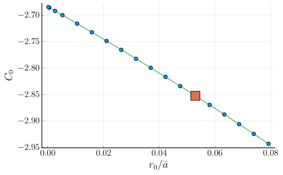
Figure 1: Running of the dimensionless constant $C_{0}=V_{0}/(\hbar^{2}/mr_{0}^{2})$ as a function of $r_{0}/\bar{a}$ at fixed scattering length $\bar{a}=189.415~{}a_{0}$. The points correspond to the calculated values, while the solid line is a quadratic fit. The limit value for $r_{0}/\bar{a}\rightarrow 0$ is $C_{0}=-2.68402(3)$, and it is in agreement with the previous results in literature Álvarez-Rodríguez et al. (2016); Bazak et al. (2016); Kievsky et al. (2017b). The square point shows the ratio at which $\bar{a}_{B}$ and $\bar{r}_{e}$ are well reproduced.

Varying the ratio $r_{0}/\bar{a}$, the effective range, the binding length, and $r_{B}$ could differ from the LM2M2 values. For instance, in the scaling limit $a_{B}\rightarrow\bar{a}$ with

$$r_{B}\sim 0.7179\,r_{0}\,,$$ (5)

and, as anticipated, the second pole of the $S$-matrix, which is proportional to $1/r_{B}$, is sent to infinity. If we want to describe this pole, both the Gaussian strength and the range have to be fine tuned

$$V_{0} =-1.22717064~{}\text{K}$$ (6)

$$r_{0} =10.03018708~{}a_{0}\,,$$

which corresponds,in Fig. 1, to the square point at $r_{0}/\bar{a}=5.29535\cdot 10^{-2}$ and $C_{0}=-2.85248$.

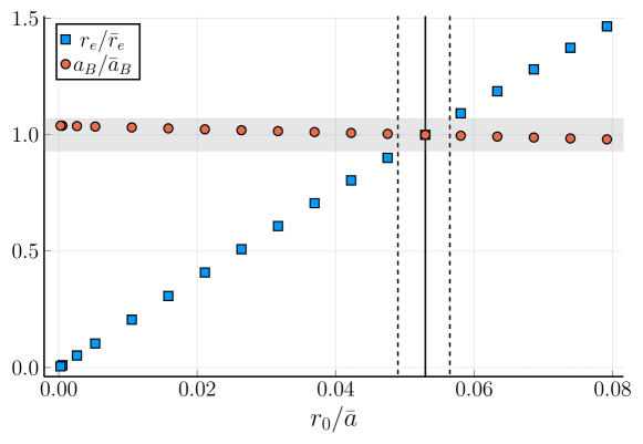
Figure 2: The ratios $a_{B}/\bar{a}_{B}$ (red circles) and $r_{e}/\bar{r}_{e}$ (blue squares) as a function of the Gaussian range $r_{0}$ (in units of $\bar{a}$). The gray band represent the $\varepsilon=7\%$ departure from the LM2M value. The binding length $a_{B}$ is always inside the LO-$\varepsilon$ band, while there is only small range of $r_{0}/\bar{a}$, identified by the two vertical dashed lines, that allows the effective range to be inside that band. Inside this range there is a special point $r_{0}/\bar{a}=5.29535\cdot 10^{-2}$, identified by the vertical solid line, where $\bar{a}$, $\bar{a}_{B}$, and $\bar{r}_{e}$ are simultaneously reproduced.

Values of $r_{e}$ and $a_{B}$ along the flux are shown in Fig. 2, where the red circles represent the ratio of the binding length with respect to the LM2M one, $a_{B}/\bar{a}_{B}$, while the blue square points represent the ratio of the effective range with respect to the LM2M one, $r_{e}/\bar{r}_{e}$. The gray band indicates the $\varepsilon\approx 7\%$ departure from the LM2M2 value, that one could consider the prediction strip for a LO description with a small parameter $\varepsilon$. The binding length is predicted inside that zone all along the flux, while there is only a small range of $r_{0}/\bar{a}$ for which also the effective range resides inside the LO 7% band. Inside this range, which is represented by the two vertical-dashed lines in Fig. 2, there is the special point for which the LO predictions exactly match the LM2M2 values.

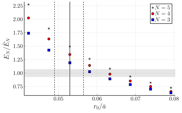
Figure 3: The ratio of the LO ground-state energy with respect to the LM2M2 value for three $E_{3}/\bar{E}_{3}$ (blue squares), four $E_{4}/\bar{E}_{4}$ (red circles), and five $E_{5}/\bar{E}_{5}$ (black stars) particle clusters. The gray band represent the $\varepsilon=7\%$ departure from the LM2M value. The vertical lines are the same as in Fig. 2; the two dashed lines delimit the range where the effective range is reproduced within the 7% and the solid line indicates the $r_{0}/\bar{a}$ value for which all the two-body LM2M2 data are reproduced.

We extend the exploration of the LO description to $N$-body clusters, limiting ourselves to the two-body potential. In Fig. 3 we show the trend for the three-, four-, and five-particle ground-state energies scaled with the LM2M2 values given in Table 1. We clearly see that as $r_{0}\rightarrow 0$ (scaling limit), $E_{N}\rightarrow\infty$, because of the well known Thomas collapse Thomas (1935). We also note that even if we fine-tune the value of the cut-off $r_{0}$ inside the range marked by the two vertical-dashed lines, where we reproduce the two-body observables, the three- and four-body data are not reproduced within the LO. Moreover, we observe that the distance from the LM2M2 value grows as a function of the size of the cluster even if we fix the value of the cut-off. In fact, in the thermodynamical limit, $N\rightarrow\infty$ there is a collapse of the system for all finite values of the Gaussian range $r_{0}$. We can use the Hyperspherical Harmonics $K=0$ approximation to give a variational bound to the energy of the clusters in the $N\rightarrow\infty$ limit ; the ground-state energy per particle is bounded from above by

$$\frac{E_{N}}{N}=\frac{V_{0}}{2}N\,,$$ (7)

showing that in this limit the system is unstable. This can be taken as a complementary evidence that in the LO description, even at finite cut-off, the theory needs a three-body force to stabilize the continuum limit of the system.

II.2 Three-body force

From the above discussion we have observed that using a Gaussian potential to describe the LO and taking the limit $r_{0}/a\rightarrow 0$, the three-body ground-state energy $E_{3}$ diverges as $1/r_{0}^{2}$. Furthermore, if the Gaussian range is fixed to describe the two-pole structure of the $S$-matrix choosing the values given in Eq. (6), we still observe the collapse given by Eq. (7) as $N\rightarrow\infty$. On the other hand we would like to see, using the inspired EFT potential at LO, all the particle sectors up to the continuum limit described inside the LO prediction. For instance, at the point fixed by Eq. (6) even the three-body bound state, $E_{3}=-150.57$ mK, is outside the LO band, as one can see in Fig. 3. Following the EFT prescription we include a three-body force at LO and proceed with computation of the ground state energies of the $N$-body clusters. The three-body force is chosen of the following from

$$W_{\text{LO}}=W_{0}\,e^{-(r_{12}^{2}+r_{13}^{2}+r_{23}^{2})/\rho_{0}^{2}}\,,$$ (8)

with $r_{ij}$ the distance between particle $i$ and particle $j$, $W_{0}$ the strength, and $\rho_{0}$ the range of the force. The force is determined by one three-body datum, to this purpose we use the $E_{3}$ ground-state energy obtained with the LM2M2. It should be noticed that in EFT the range $\rho_{0}$ is sent to zero together with $r_{0}$. In the following we analyze the dependence of $E_{N}$ on different choices of $r_{0}$ and $\rho_{0}$. The resulting limit cycle in the renormalization group flow has been recently studied Recchia et al. (2022). Here we determine different combinations of $(V_{0},r_{0})$ values, all of them reproducing the two-body scattering length $\bar{a}$. For each pair we associate a family of pair values $(W_{0},\rho_{0})$ leading to the same three-body binding energy $E_{3}$.

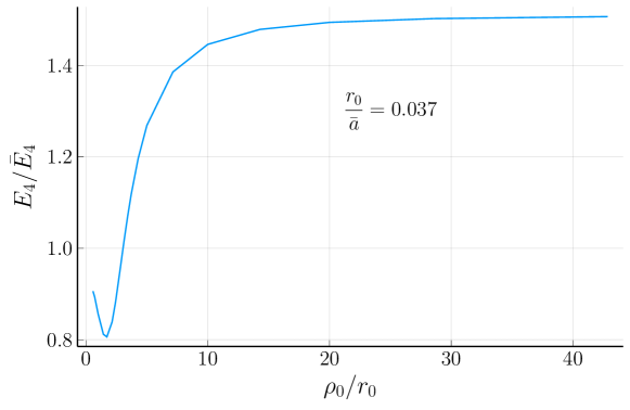
Figure 4: The ratio $E_{4}/\bar{E}_{4}$ as a function of $\rho_{0}/r_{0}$. In the figure, the specific case $r_{0}/\bar{a}=0.037$ is shown. For each value of $\rho_{0}$, the three-body strength $W_{0}$ has been fixed in order to verify $E_{3}/\bar{E}_{3}=1$. The ratio $E_{4}/\bar{E}_{4}$ varies between two values, and if the minimum is below one, there is a special value of the pair $(W_{0},\rho_{0})$ for which $E_{4}/\bar{E}_{4}=1$.

We would like to show that inside these families of pairs there is a best choice which allows for the optimum description of the multi-particle sectors, starting from the four-particle one Gattobigio et al. (2011); Kievsky et al. (2020). This can be seen in Fig. 4, where the ratio $E_{4}/\bar{E}_{4}$ is calculated as a function of $\rho_{0}/r_{0}$; the ratio has a bell-type shape and it varies between a minimum, which is usually attained for $\rho_{0}/r_{0}\sim 1$, and a maximum in the limit of $\rho_{0}/r_{0}\rightarrow+\infty$, where the three-body force tends to be a constant (the difference between $\bar{E}_{3}$ and the three-body ground-state energy without the three-body force). In the figure we have selected the value $r_{0}/\bar{a}=0.037$, however this behavior is similar for different ratios and for different particle sectors.

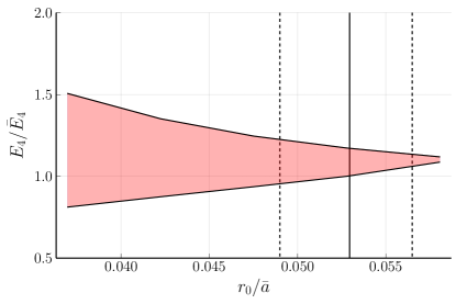
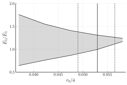
Figure 5: Range of variability of the ratios $E_{4}/\bar{E}_{4}$ (left panel) and $E_{5}/\bar{E}_{5}$ (right panel) as a function of the two-body range $r_{0}/\bar{a}$. For a fixed value of $r_{0}/\bar{a}$, the range of variability is given by the maximum and the minimum of the curve as given in Fig. 4 for one case. The vertical lines have the same meaning as in Fig. 2. For $r_{0}/\bar{a}\lesssim 0.053$, on the left of the solid-vertical line, it is possible to fix either $E_{4}/\bar{E}_{4}=1$ or $E_{5}/\bar{E}_{5}=1$ with a suitable choice of the $(W_{0},\rho_{0})$ pair.

In Fig. 5 we report the bands inside which the ratios $E_{4}/\bar{E}_{4}$ and $E_{5}/\bar{E}_{5}$ of four and five particles respectively, can be found as the ratio $\rho_{0}/r_{0}$ varies from its lower to its maximum value. We observe that for $r_{0}/\bar{a}$ values at the left of the special point given in Eq. (6), and represented in Fig. 5 by the solid-vertical line, it is possible to fix the pair $(W_{0},\rho_{0})$ in order to reproduce either the four- or the five-body ground-state energy.

To analyze further this fact, we tune the pairs $(W_{0},\rho_{0})$ to have $E_{4}/\bar{E}_{4}=1$ whenever is possible, namely for $r_{0}/\bar{a}\lesssim 0.053$. In the other cases the ratio $E_{4}/\bar{E}_{4}$ is set as close as possible to 1. With this prescription we calculate the ground-state energy for $N=5,6,7$ clusters and the results are shown in Fig. 6. Analysing the figure from the left to the right, we observe that the few-body ground-state energies tends to converge to the LM2M2 data as we move toward the special value of $r_{0}/\bar{a}$. Around this point, the predicted energies are well inside the $\varepsilon=7\%$ deviation from LM2M2 data maintaining the LO accuracy. This point has been already noticed in Ref. Kievsky et al. (2020) where a different helium potential has been used as reference. Moreover, in Ref. Kievsky et al. (2020) it has been shown that also the saturation energy is predicted within the LO uncertainty. The present analysis extends these findings showing that there is a small range of values of the cut-offs, $r_{0}$ and $\rho_{0}$, allowing for a LO accuracy of the energy per particle $E_{N}/N$.

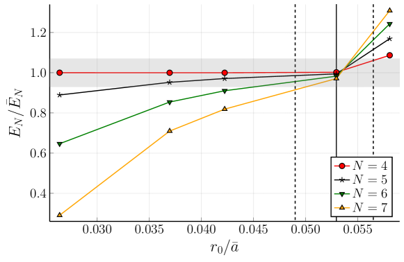
Figure 6: The ratios $E_{N}/\bar{E}_{N}$ for $N=4,5,6,7$ are given as a function of $r_{0}/\bar{a}$. The three-body force has been fixed by imposing $E_{4}/\bar{E}_{4}$ as close as possible to 1. The vertical lines are the same as in Fig. 2, and the gray strip corresponds to the $\varepsilon=7\%$ departure from LM2M2 data. When the four-body energy $E_{4}=\bar{E}_{4}$, the five- and six-body clusters are found to be less bound than the LM2M2 data, with the best description at the point given by Eq. (6), i.e. where the second pole of the $S$-matrix is well described. In this point the predictions are all inside the $\varepsilon$-LO strip. For $r_{0}/\bar{a}>0.053$ the opposite trend is verified.

III Next-to-leading order description

In this section we introduce the next-to-leading order (NLO) term of the EFT inspired potential. At this order we expect to increase the accuracy of the description at the level of $\varepsilon^{2}\approx 5\permil$.

III.1 Two-body force

Following the same counting criterion of EFT Epelbaum et al. (2017), the two-body NLO potential is

$$V_{\text{NLO}}(r)=V_{0}\,e^{-(r/r_{0})^{2}}+V_{1}\,\frac{r^{2}}{r_{0}^{2}}e^{-(r/r_{0})^{2}}\,,$$ (9)

where the additional term is proportional to the square-particle distance. In the following the range of the two Gaussian functions are kept equal, but clearly this is not the only possible choice Epelbaum et al. (2018).

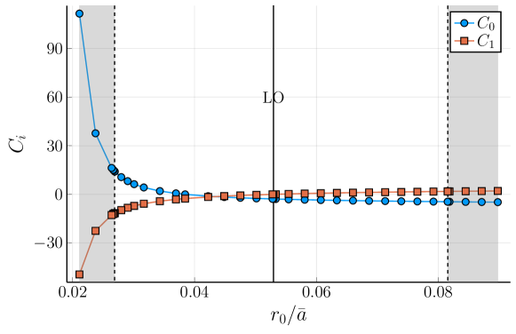
Figure 7: Running of the dimensionless constants $C_{0}=V_{0}/(\hbar^{2}/mr_{0}^{2})$ and $C_{1}=V_{1}/(\hbar^{2}/mr_{0}^{2})$ as a function of $r_{0}/\bar{a}$ at fixed scattering length $\bar{a}=189.415~{}a_{0}$ and effective range $\bar{r}_{e}=13.845~{}a_{0}$. The gray zones correspond to $E_{3}/\bar{E}_{3}<1$. The vertical-dashed lines indicate the two values of $r_{0}/\bar{a}$ where $E_{3}/\bar{E}_{3}=1$. The center-dashed line shows the $C_{1}=0$ case, where the LO and the NLO potentials concide.

For different choices of the range $r_{0}$, the NLO potential has two LECS, $V_{0}$ and $V_{1}$. There is a whole family of strength values which allows to reproduce the structure of the $S$-matrix given in Eq. (1). Introducing the dimensionless strengths $C_{0}=V_{0}/(\hbar^{2}/mr_{0}^{2})$ and $C_{1}=V_{1}/(\hbar^{2}/mr_{0}^{2})$, we fix them as a function of the range $r_{0}/\bar{a}$ to reproduce both the scattering length $\bar{a}$ and the effective range $\bar{r}_{e}$. In Fig. 7 we trace the two strengths (or LECs), $C_{0}$ and $C_{1}$ as a function of $r_{0}/\bar{a}$. We observe that there is a special point, indicated by the vertical-solid line (labeled LO), where $C_{1}=0$ and the NLO description coincides with the LO description of Eq. (6). In addition, there are two special points, marked by the two vertical-dashed lines, where $E_{3}/\bar{E}_{3}=1$. In this case the three-body force should give a null contribution to the three-body ground state. Beyond these lines, we have the zone where $E_{3}/\bar{E}_{3}>1$ indicated by the gray strips, for which an attractive three-body force is needed. The scaling limit of $C_{0}$ and $C_{1}$ is not finite; both LEC’s have an essential singularity at $r_{0}=0$, $C_{i}\sim\exp[\alpha_{i}(\bar{a}/r_{0})+\beta_{i}(\bar{a}/r_{0})^{2}]$, as can be clearly seen from Fig. 8 ($\alpha_{i}$ and $\beta_{i}$ are fitting constants).

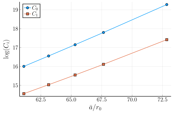
Figure 8: The log-behavior of the LECs as a function of $\bar{a}/r_{0}$ for small values of $r_{0}$. The two curves can be fitted using a polynomial of degree two, showing that $C_{i}\sim\exp(\alpha_{i}(\bar{a}/r_{0})+\beta_{i}(\bar{a}/r_{0})^{2}$.

The family of potentials having the same scattering length and the same effective range, but different range, are not phase equivalents; they develop different shape parameters. In Fig. 9 the two-body potential is plotted for three different values of $r_{0}$, corresponding to the cases where they give $E_{3}/\bar{E}_{3}=1$ (left and right plot), and to the special LO point of Eq. (6) (center plot) which is also NLO. Interestingly, as $r_{0}/\bar{a}\rightarrow 0$, the potential develops a repulsive core which mimics the LM2M2 one, however this feature is not enough to prevent the collapse of the $N\rightarrow\infty$ system. This behavior is illustrated in Fig. 10 where we show $E_{N}/\bar{E}_{N}$ for $N=3,4,5,6$. As the number of particles grows, the ratio $E_{N}/\bar{E}_{N}$ increases indicating the instability in the $N\rightarrow\infty$ limit. In particular this is the case for the lowest value analyzed, $r_{0}/a_{0}=5.093$, corresponding to the case $E_{3}/\bar{E}_{3}=1$. This instability can be further analyzed using the HH $K=0$ approximation which gives the asymptotic variational estimate of the energy per particle as proportional to the number of particles Note (1),

$$\frac{E_{N}}{N}\propto N\,.$$ (10)

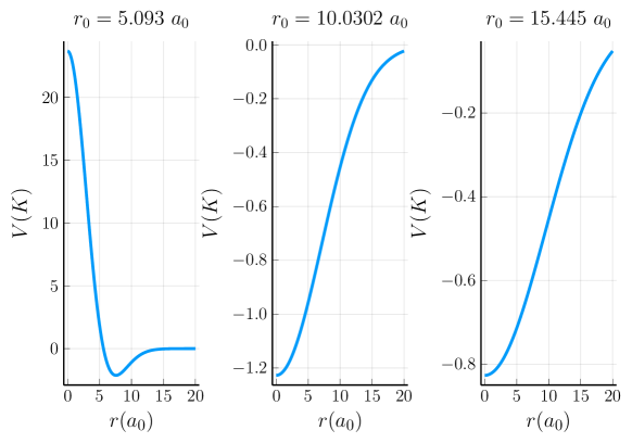
Figure 9: Profile of the NLO potentials for the three different values of $r_{0}$. The left and right panels correspond to the two extreme cases where the NLO potential reproduce the three-body ground-state energy. These two points are indicated by the vertical-dashed line in Fig. 7. The central panel corresponds to the NLO-LO case (vertical-solid line in Fig. 7).

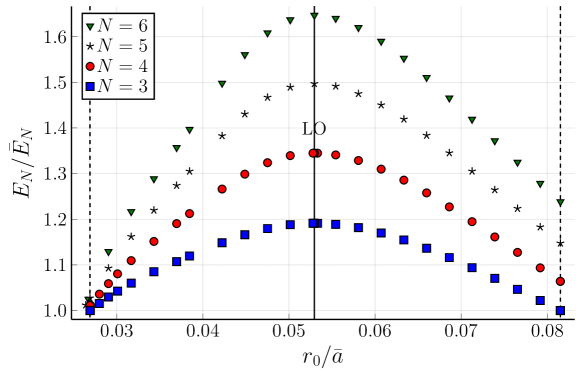
Figure 10: The ground-state energy $E_{N}$ (in units of $\bar{E}_{N}$). computed with the NLO two-body force of Eq. (9). The vertical lines are the same as in Fig. 7.

III.2 Three-body force

Contrary to the LO case, the three-body ground state calculated with two-body NLO potential does not collapse as $r_{0}\rightarrow 0$. Approaching this limit the two-body potential develops a repulsive core, a consequence of the two parameters, the scattering length and the effective range, it has to reproduce. For $r_{0}/a$ values inside the region verifying $E_{3}/\bar{E}_{3}\geq 1$, the deepest energy corresponds to the particular case in which $V_{1}=0$ and the LO and NLO potentials coincide. This is true also for $N>3$ as shown in Fig. 10 where the binding energies for $N=3,4,5,6,7$ are shown, in units of $\bar{E}_{N}$, as functions of the Gaussian range $r_{0}$, in units of $\bar{a}$. A demonstration of why the deepest energy is reach in that particular point is given in the Appendix A.

We proceed the study by considering the two-body NLO potential plus the LO three-body force of Eq. (8). To this end we compute pairs of $(W_{0},\rho_{0})$ values from the condition $E_{3}/\bar{E}_{3}=1$. We select the best pair of values by analyzing the four-body ground-state energy and, using this choice, we calculate the $N=5,6,7$ binding energies. The results are reported in Fig. 11, where we show the ratios $E_{N}/\bar{E}_{N}$ for $N=4,5,6,7$ as functions of $r_{0}/\bar{a}$ inside the region in which the three-body force is repulsive. Firstly we observe that, although $E_{4}$ is very close to the exact value, it is not possible to set $E_{4}/\bar{E}_{4}=1$; the best value is obtained for the NLO-LO point given by Eq. (6) and it is inside the $\varepsilon^{2}=5\permil$ deviation from the LM2M2 value. The $E_{4}/\bar{E}_{4}$ ratio remains close to 1 inside the region between the NLO-LO point and the lower value of $r_{0}/\bar{a}$ for which the three-body binding energy is well reproduced by solely the NLO two-body potential. In between these points, there is a special value of $r_{0}/\bar{a}\approx 0.042$ (and $\rho_{0}/r_{0}\approx 7/8$) such that all the $N$-body systems (at least up to seven particles) have a ground-state energy which is inside the NL0-$\varepsilon^{2}$ strip. There is a similar point for the higher value $r_{0}/\bar{a}\approx 0.063$ (and $\rho_{0}/r_{0}\approx 7/12$). At these two points, the binding energies, $E_{N}$ with $N\leq 7$ are predicted inside the $5\permil$ strip.

Now we look at the two points, $r_{0}/\bar{a}=0.027$ and $0.081$, characterized by the fact that the three-body binding energy is well reproduced by the two-body NLO potential. Accordingly the contribution of the three-body force, in the three-body system, should be zero. However, if we consider only the two-body NLO potential and use the HH $K=0$ approach to estimate the limit $N\rightarrow\infty$ we can show that the system is unstable Note (1). Therefore we conclude that the three-body force should have at least two terms that compensate each other to give zero contribution in the three-body system but non-zero ones for $N>3$ and stabilizes the systems as $N$ increases. To analyse this behavior we introduce the following NLO three-body force

$$W_{\text{NLO}}=W_{0}e^{-r_{123}^{2}/\rho_{0}^{2}}+W_{1}\left(\frac{r_{123}}{\rho_{0}}\right)^{2}e^{-r_{123}^{2}/\rho_{0}^{2}}\,,$$ (11)

where $r_{123}^{2}=r_{12}^{2}+r_{13}^{2}+r_{23}^{2}$. To be noticed that in a perturbative scheme the $W_{1}$ term can be absorbed by the LO term Hammer and Mehen (2001); Bedaque and van Kolck (2002). In this case, and as discussed in Ref. Bazak et al. (2019), a subleading four-body interaction could be introduced. Using a non-perturbative scheme, the two LECs $W_{0}$ and $W_{1}$ are independent. In order to determine possible values of the additional LEC, $W_{1}$, we compute pairs of $W_{0},W_{1}$ values obtained through the condition $E_{3}=\bar{E}_{3}$. Next, we study the effects of the different pairs in the binding energies $E_{N}$ with $N\leq 7$.

We now extend the study to consider the complete NLO potential consisting in a two plus a three-body term. The results are shown in Fig. 12, where the ratios $E_{N}/\bar{E}_{N}$ and $a_{2}/\bar{a}_{2}$ are given as a function of the gaussian range $r_{0}$, in units of $\bar{a}$. From the figure we can conclude that the NLO force is sufficiently flexible to describe accurately the $E_{N}$ binding energies inside the region in which the three-body force has an overall repulsive contribution including the point in which it has a null contribution to the three-body system. All the binding energies fall inside (or very close to) the $5\permil$ strip. To obtain these results the three-body range $\rho_{0}$ has been varied and, for each value of $r_{0}$, the selected value is the one that gives the best results. This fact implies that the two ranges, $r_{0}$ and $\rho_{0}$, are correlated and need to be tuned simultaneously to optimize the capability of the force to describe systems having different values of $N$. For each value of $r_{0}$ there is a particular value of $\rho_{0}$ that produce the best results for the binding energies. We infer that this value is not universal, it takes into account the short range characteristics of the systems trying to adapt the (repulsive) three-body force in order to reproduce the packing of the particles as $N$ increases. It seems that this behavior, for one specific value of $r_{0}$, can be codified in one particular value of $\rho_{0}$.

Finally we incorporate in the study the atom-dimer scattering length $a_{2}$. This observable will give additional information on the capability of the NLO potential to describe the few-body dynamics. In Fig. 13 we report a preliminary analysis of the ratio $a_{2}/\bar{a}_{2}$, where $\bar{a}_{2}=218.0~{}a_{0}$ is the LM2M2 atom-dimer scattering length. In the figure we show the results including the two-body NLO force (green symbols), when the LO three-body force is also included (blue symbols) and when NLO three-body is considered as well (red symbols). In the first case we see that there is a parabolic behavior with the minimum just in the LO/NLO point corresponding to $r_{0}/\bar{a}=0.053$. This behavior is maintained when the LO three-body force is included though with less variation in all the region analyzed. When the NLO three-body force is included the observable is well inside the expected error band.

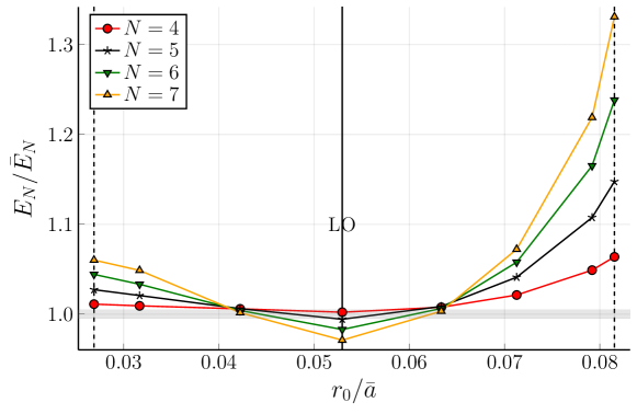
Figure 11: The ratios $E_{N}/\bar{E}_{N}$ for $N=4,5,6,7$ as a function of $r_{0}/\bar{a}$ computed with the two-body force at NLO and the three body force at LO. The three-body force has been fixed to have the best $E_{4}/\bar{E}_{4}$ ratio, which is always larger than 1. The vertical lines are the same as in Fig. 7. The horizontal gray strip corresponds to the $\varepsilon^{2}=5\permil$ departure from LM2M2 data. The point where $E_{4}/\bar{E}_{4}$ is closer to 1 is the NLO-LO point given by Eq. (6).

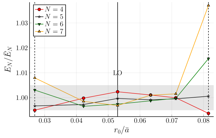
Figure 12: The ratios $E_{N}/\bar{E}_{N}$ for $N=4,5,6,7$ as a function of $r_{0}/\bar{a}$ computed with the two-body and three-body forces at NLO. The three-body force parameters have been fixed to have $E_{3}/\bar{E}_{3}=1$ and the best $E_{4}/\bar{E}_{4}$ ratio. The vertical lines are the same as in Fig. 7. The horizontal gray strip corresponds to the $\varepsilon^{2}=5\permil$ departure from LM2M2 data. The results stay inside the expected error band for values of $r_{0}/\bar{a}$ close to the LO vaue.

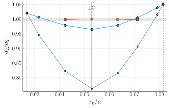
Figure 13: The atom-dimer scattering length, $a_{2}$ (in units of the LM2M2 atom-dimer scattering length $\bar{a}_{2}=218.0~{}a_{0}$), as a function of $r_{0}/\bar{a}$. The calculations have been done using the tewo-body NLO potential (green symbols), including the the LO three-body force (blue symbols) and the NLO three-body force (red symbols). The vertical lines are the same as in Fig. 7, and the horizontal gray strip gives the $\varepsilon^{2}=5\permil$ deviation.

IV Conclusions and Outlooks

We have studied in detail how the leading order and the next to leading order interactions of a boson system can be built by looking to a few data. In the LO case we have looked at the two-body scattering length and the trimer energy whereas at NLO we have considered the effective range and the tetramer binding energy (or the atom-dimer scattering length). The ranges of the associated potentials (of a Gaussian shape) have been varied inside certain regions. At LO we have shown that, if we want to maintain similar level of accuracy in the description of systems with increasing values of $N$, the possible values of $r_{0}$ and $\rho_{0}$ are very few. In fact, as it is evident from Fig. 6, there is only one possible pair of values, $r_{0}$ and $\rho_{0}$, that respects this condition. Moreover the value of $r_{0}$ is the one that allows a simultaneously description of the two-body scattering length and of the effective range. This is an important finding since this particular value of $r_{0}$ gives the correct description of the two-pole structure of the $S$-matrix showing the strict correlation that this structure introduces in heavier systems. Moreover, associated to that particular $r_{0}$ value, there is a particular value of the three-body potential range $\rho_{0}$ that takes into account the correct balance between attraction and repulsion along the energy curve $E_{N}$ as a function of $N$. That particular value of $\rho_{0}$ governs the transition from universal to non-universal effects in which the short-range characteristic of the interaction prevents the system to collapse (see the related discussions in Refs. Kievsky et al. (2017a, 2018, 2021b, 2020)).

The LO description establishes the level of accuracy required in the description of the binding energies. A consistent improvement is expected once the next-to-leading order is considered. The first finding in this analysis was the observation that the two-body NLO potential produces a maximum (in absolute value) in the description of the binding energies, $E_{N}$, with $N\geq 3$, located at the particular point in which the second LEC of the potential $V_{1}=0$. At this point the NLO potential consists in a single Gaussian, and by definition, its range is the one needed to describe, in addition to the scattering length, the effective range. As soon as $r_{0}$ is varied from that value the trimer energy increases arriving to two values at which the trimer energy is well described, $E_{3}=\bar{E}_{3}$. Beyond these values the three-body force should be attractive, a situation that without other intervening mechanisms would produce a collapse of the system. So, in the present analysis we have studied the NLO force inside those limits.

The next step in this study was the introduction of the three-body potential. To start with, in Fig. 11 we have analysed the NLO two-body force in conjunction with the three-body force at LO. This analysis shows a limited improvement of the description, mostly around two points, at $r_{0}/\bar{a}\approx 0.042$ and $0.063$. At these two points the description of the binding energies up to $N=7$ remains inside the expected level of confidence. The final results are shown in Fig. 12 in which the complete NLO force has been considered. Noticeably the complete segment of $r_{0}/\bar{a}$ values allows for a description of the binding energies inside the error strip. However, as mentioned before, at each point it was necessary to set the value of $\rho_{0}$. So we have shown that there is a strict correlation between the two-body range $r_{0}$ and the three-body range $\rho_{0}$. Similar conclusions are obtained analysing the results for the atom-dimer scattering length. This fact has been observed at LO in fermionic systems Kievsky et al. (2018); Schiavilla et al. (2021). Studies along the inclusion of the NLO term in such systems are at present under way.

Appendix A Special point where the two-body force at LO and NLO are the same

We show why the binding energies calculated using the two-body force at NLO have their minimum value at the particular $r_{0}$ value in which $V_{1}=0$ (see Eq.(9)). At that point the two-body potential is the same at LO and NLO. To this end we first extend the Hellmann-Feynman theorem

$$\frac{\partial E_{\lambda}}{\partial\lambda}=\langle\Psi_{\lambda}|\frac{\partial H_{\lambda}}{\partial\lambda}|\Psi_{\lambda}\rangle\,,$$ (12)

to be valid in the zero-energy case.

A.1 Hellmann-Feynman theorem for the scattering length

Here we demonstrate the validity of Hellmann-Feynman theorem in the case in which the variation is done on the scattering length. We start from the Kohn variational principle for the scattering length functional

$$[a_{\lambda}]=a_{\lambda}+\langle\psi_{\lambda}|H_{\lambda}|\psi_{\lambda}\rangle\,,$$ (13)

where $[a_{\lambda}]$ is the second order estimate and $\psi_{\lambda}$ is normalized so that $\psi_{\lambda}\rightarrow F+a_{\lambda}G$, with $F,G$ the regular and irregular asymptotic solutions. Now the variation of the functional with respect to $\lambda$ is

$$\frac{\partial[a_{\lambda}]}{\partial\lambda}=\frac{\partial a_{\lambda}}{\partial\lambda}+\langle\frac{\partial\psi_{\lambda}}{\partial\lambda}|H_{\lambda}|\psi_{\lambda}\rangle+\langle\psi_{\lambda}|\frac{\partial H_{\lambda}}{\partial\lambda}|\psi_{\lambda}\rangle+\langle\psi_{\lambda}|H_{\lambda}|\frac{\partial\psi_{\lambda}}{\partial\lambda}\rangle\,.$$ (14)

From the normalization condition we can observe that

$$\langle\frac{\partial\psi_{\lambda}}{\partial\lambda}|H_{\lambda}|\psi_{\lambda}\rangle-\langle\psi_{\lambda}|H_{\lambda}|\frac{\partial\psi_{\lambda}}{\partial\lambda}\rangle=\frac{\partial a_{\lambda}}{\partial\lambda}$$ (15)

and therefore

$$\frac{\partial[a_{\lambda}]}{\partial\lambda}=2\langle\frac{\partial\psi_{\lambda}}{\partial\lambda}|H_{\lambda}|\psi_{\lambda}\rangle+\langle\psi_{\lambda}|\frac{\partial H_{\lambda}}{\partial\lambda}|\psi_{\lambda}\rangle=\langle\psi_{\lambda}|\frac{\partial H_{\lambda}}{\partial\lambda}|\psi_{\lambda}\rangle$$ (16)

where we have used that $H_{\lambda}|\psi_{\lambda}\rangle=0$. Accordingly, the extension of the Hellmann-Feynman theorem to the case of a zero-energy state results to be:

$$\frac{\partial[a_{\lambda}]}{\partial\lambda}=\langle\psi_{\lambda}|\frac{\partial H_{\lambda}}{\partial\lambda}|\psi_{\lambda}\rangle$$ (17)

A.2 Minimum of $V_{0}$ for $V_{1}=0$.

It is interesting to analyse why the minimum value of $E_{N}$ corresponds to the case in which the LO and NLO two-body potentials are the same potential. In particular we observe that at that point $V_{0}$ has its minimum value. We start from the two-body NLO hamiltonian

$$H^{\text{NLO}}_{r_{0}}=T+V^{\text{NLO}}\,,$$ (18)

where we have made explicit the $r_{0}$ dependence. Now we recall the Hellmann-Feynman theorem

$$\frac{\partial E_{\lambda}}{\partial\lambda}=\langle\Psi_{\lambda}|\frac{\partial H_{\lambda}}{\partial\lambda}|\Psi_{\lambda}\rangle\,,$$ (19)

for a general dependence of the hamiltonian on the parameter $\lambda$ and the corresponding wave function $\Psi_{\lambda}$. Its extension to the case of the scattering length is

$$\frac{\partial a_{\lambda}}{\partial\lambda}=\langle\psi_{\lambda}|\frac{\partial H_{\lambda}}{\partial\lambda}|\psi_{\lambda}\rangle\,,$$ (20)

where now $\psi_{\lambda}$ is the zero-energy wave function (a demonstration of the theorem for scattering states is given above). In our case $\lambda\equiv r_{0}$ and due to the constrains, $E_{2}$ and $a$ are maintained constants as $r_{0}$ is varied, the variations of $E_{2}$ and $a$ with respect to $r_{0}$ are zero. Explicitly

$$\frac{\partial E_{2}}{\partial r_{0}} =0=\langle\Psi_{r_{0}}|\frac{\partial H^{\text{NLO}}_{r_{0}}}{\partial r_{0}}|\Psi_{r_{0}}\rangle=\langle\Psi_{r_{0}}|\frac{\partial V^{\text{NLO}}}{\partial r_{0}}|\Psi_{r_{0}}\rangle$$ (21)

$$=\langle\Psi_{r_{0}}|\left(\frac{\partial V_{0}}{\partial r_{0}}+2V_{0}\frac{r^{2}}{r_{0}^{3}}\right)e^{-(r^{2}/r_{0}^{2})}+\left(\frac{\partial V_{1}}{\partial r_{0}}\frac{r^{2}}{r_{0}^{2}}-2V_{1}\frac{r^{2}}{r_{0}^{3}}+2V_{1}\frac{r^{4}}{r_{0}^{5}}\right)e^{-(r^{2}/r_{0}^{2})}|\Psi_{r_{0}}\rangle\,,$$

where $\Psi_{r_{0}}$ is the bound state wave function. We are interested in the point in which $V_{1}=0$, therefore the equation is

$$\frac{\partial V_{0}}{\partial r_{0}}\langle\Psi_{r_{0}}|e^{-(r^{2}/r_{0}^{2})}|\Psi_{r_{0}}\rangle+\left(\frac{2V_{0}}{r_{0}}+\frac{\partial V_{1}}{\partial r_{0}}\right)\langle\Psi_{r_{0}}|\frac{r^{2}}{r_{0}^{2}}e^{-(r^{2}/r_{0}^{2})}+|\Psi_{r_{0}}\rangle=0\,,$$ (22)

and a similar equation for the zero-energy wave function, $\psi_{r_{0}}$

$$\frac{\partial V_{0}}{\partial r_{0}}\langle\psi_{r_{0}}|e^{-(r^{2}/r_{0}^{2})}|\psi_{r_{0}}\rangle+\left(\frac{2V_{0}}{r_{0}}+\frac{\partial V_{1}}{\partial r_{0}}\right)\langle\psi_{r_{0}}|\frac{r^{2}}{r_{0}^{2}}e^{-(r^{2}/r_{0}^{2})}+|\psi_{r_{0}}\rangle=0\,.$$ (23)

Since $\Psi_{r_{0}}$ and $\psi_{r_{0}}$ are orthogonal, the gaussian matrix elements cannot be linear dependent and therefore the only possibility is that each coefficient is zero. In particular the following condition is verified

$$\frac{\partial V_{0}}{\partial r_{0}}=0\,,$$ (24)

together with $2V_{0}/r_{0}+\partial V_{1}/\partial r_{0}=0$. These conditions indicate that when the variation is performed on $E_{N}$ it results

$$\frac{\partial E_{N}}{\partial r_{0}}=0$$ (25)

at the $V_{1}=0$ point. This behavior can be observed in Fig.10 for $N=3,4,5,6$.