TESS Hunt for Young and Maturing Exoplanets (THYME) VII : Membership, rotation, and lithium in the young cluster Group-X and a new young exoplanet

Abstract

The public, all-sky surveys Gaia and TESS provide the ability to identify new young associations and determine their ages. These associations enable study of planetary evolution by providing new opportunities to discover young exoplanets. A young association was recently identified by Tang et al. and Fürnkranz et al. using astrometry from Gaia (called “Group-X” by the former). In this work, we investigate the age and membership of this association; and we validate the exoplanet TOI 2048 b, which was identified to transit a young, late G dwarf in Group-X using photometry from TESS. We first identified new candidate members of Group-X using Gaia EDR3 data. To infer the age of the association, we measured rotation periods for candidate members using TESS data. The clear color–period sequence indicates that the association is the same age as the $300\pm 50$ Myr-old NGC 3532. We obtained optical spectra for candidate members that show lithium absorption consistent with this young age. Further, we serendipitously identify a new, small association nearby Group-X, which we call MELANGE-2. Lastly, we statistically validate TOI 2048 b, which is a $2.6\pm 0.2$ $R_{\earth}$ radius planet on a 13.8-day orbit around its $300$ Myr-old host star.

1 Introduction

Age is a critical parameter that places stellar and planetary evolution on a timeline, yet it is difficult to directly observe the age of a star. Common ways to determine the ages of low-mass stars include isochrones, rotation, and Li depletion (Skumanich, 1972; Soderblom, 2010). As stars evolve toward, along, and off the main sequence, their positions in a color–absolute magnitude diagram reflect their changing ages. Rotation slows with time as a consequence of magnetized stellar winds (Schatzman, 1962; Weber & Davis, 1967), with periods converging to and then following a single color–period sequence (Barnes, 2003). Activity consequently decays due to the weakening of the magnetic dynamo at longer rotation periods (Kraft, 1967; Noyes et al., 1984). Li depletes with time due to core fusion and convective mixing, following an age- and mass-dependent color–Li sequence (Wallerstein et al., 1965; Bodenheimer, 1965). Asteroseismology provides another alternative for some stars (Chaplin & Miglio, 2013).

Co-eval stellar associations are the cornerstones of empirical age calibrations; however, we remain limited by the range of ages of observationally accessible open clusters. The Gaia mission (Gaia Collaboration et al., 2016) has enabled the discovery of new associations and expanded our knowledge of known ones, by making publicly available parallaxes, proper motions, and broadband photometry for a billion sources. For example, Meingast et al. (2019) found a previously unknown association, the Pisces-Eridanis stream, which extends 120 degrees across the sky. Meingast et al. (2021) found extended halos surrounding numerous clusters, and Röser et al. (2019) identified tidal tails of the Hyades cluster.

All-sky searches for new clusters have yielded an abundance of small groups of co-moving stars that are likely to be physically associated. For example, Oh et al. (2017) used positions and proper motions from Gaia DR1 to search for co-moving stars. Some of these stars revealed themselves to be parts of larger associations: Faherty et al. (2018) found that four were newly discovered, while the remaining 23 matched known associations. Kounkel & Covey (2019) used positions and proper motions from Gaia DR2 to search for clustering using an unsupervised machine learning algorithm. They identified 1901 groups, many of which appear filamentary.

Group-X was discovered independently by Tang et al. (2019) and Fürnkranz et al. (2019). Tang et al. (2019) serendipitously discovered the young association, which they called “Group-X,” during a search for the tidal tails of Coma Berenices, a northern open cluster about $700$ Myr old. Using STARGO (Yuan et al., 2018), an unsupervised neural net, they identified the tails of Coma Ber—and the unexpected, and unassociated, Group-X. Fürnkranz et al. (2019) searched for overdensities in velocity space following the methodology of Meingast & Alves (2019). This algorithm uses DBSCAN (Ester et al., 1996) in combination with additional filtering. Both searches were based on position and proper motion from Gaia DR2, since radial velocities were available for only about a quarter of the stars in their search space. The narrow and distinct distributions of proper motion and available radial velocities demonstrate that Coma Ber and Group-X are independent. Noting that Group-X is irregularly shaped, Tang et al. (2019) suggested that past close encounters may be responsible for disrupting the association. Fürnkranz et al. (2019) found that such encounters are likely to occur frequently.

The candidate membership lists from Tang et al. (2019, 218 stars) and Fürnkranz et al. (2019, 177 stars) overlap significantly despite the use of different algorithms. There are 21 stars that appear in Fürnkranz et al. and not Tang et al., and 62 stars that appear in Tang et al. and not Fürnkranz et al. Stars from Tang et al.’s list are more extended in proper motion.

As discussed in Tang et al. (2019), candidate Group-X members partially overlap with groups 10, 81, and 1805 from Oh et al. (2017). The largest overlap, 27 stars, was with Oh et al.’s Group 10. Faherty et al. (2018), reassessing and reorganizing the larger groups in Oh et al.’s catalog, highlight the potential interest of Group-X due to its relative richness and proximity. They also found that Group 10 was not associated with any known cluster or young moving group, though three are amongst the seven stars that Latyshev (1977) suggested as a possible cluster.

We conducted an in-depth study of Group-X, considering both its stellar population (membership and age) and the first exoplanet discovered in the group, TOI 2048 b. TOI 2048 b is a small planet found to transit its host star in data from the Transiting Exoplanet Survey Satellite (TESS; Ricker et al., 2015). The host star TOI 2048 was identified as a candidate member of Group-X by Tang et al. (2019); it falls near the edge of the group and was not identified as a member by Fürnkranz et al. (2019).

We present our observations of TOI 2048 and candidate members of Group-X in Section 2, and a detailed analysis of the host star TOI 2048 in Section 3. In Section 4 we identify candidate new members of Group-X and use stellar rotation and lithium to constrain the association’s age. We turn to characterization of the planet in Section 5, and conclude in Section 6.

This work is part of the TESS Hunt for Young and Maturing Exoplanets (THYME; Newton et al., 2019; Mann et al., 2020) Survey. The goal of THYME is to use the partnership between stellar and exoplanet science to support the discovery and characterization of young planets (e.g. Newton et al., 2021; Tofflemire et al., 2021); TOI 2048 and Group-X highlight this synergy well.

2 Observations of TOI 2048 and Group-X candidate members

2.1 Time-series photometry

2.1.1 Space based photometry from TESS

TOI 2048 was observed in sectors 16 (12 September 2019 to 6 October 2019), and 23–24 (19 March 2020 to 12 May 2020) during TESS’s second year of operations. Data from the Quick Look Pipeline (QLP; Fausnaugh et al., 2020; Huang et al., 2020a, b) was used to initially identify the planet candidate, which was announced via the alerts as TOI 2048.01 (Guerrero et al., 2021).

We used two-minute cadence data produced by the Science Processing and Operations Center (SPOC; Jenkins et al., 2016) and thirty minute cadence data produced by a custom pipeline operating on the full-frame images (FFIs). We used lightkurve (Lightkurve Collaboration et al., 2018) to access SPOC data. The SPOC pipeline produces two data products (Jenkins, 2015; Jenkins et al., 2016). The simple aperture photometry (SAP data, Twicken et al. 2010; Morris et al. 2020) includes calibration, extraction, and background subtraction. The pre-search data conditioning simple aperture photometry (PDCSAP data, Stumpe et al. 2012, 2014; Smith et al. 2012) additionally removes instrumental systematics using cotrending basis vectors. A strong systematic arises from scattered light, which includes signals at 1 and 14 days.

The TESS data for TOI 2048 and Group-X members are strongly affected by systematics, and the PDCSAP corrections did impact the observed stellar rotation signal in some cases. The particular regime in which this matters is stars with rotation periods ($P_{\star}$) between about 6 and 12 days, for which PDCSAP corrections can modify the rotational variability such that the apparent period is $P_{\star}/2$. This is illustrated in Figure 1. Similar behavior was noted in one target from Magaudda et al. (2021); our investigation shows that this is prevalent, at least in some sectors. Additionally, the PDC data for TOI 2048 shown in Figure 1 displays some abrupt jumps not seen in the SAP data. We therefore used SAP data instead of PDCSAP data for our analyses.

The SAP data has not been corrected for crowding, but crowding is negligible for this source (0.5% in the most contaminated sector). Data from these sectors were also processed with the original version of the sky background algorithm, which can result in significant over-correction of the background flux. We analyzed the target pixel files for this star and found that the bias in the transit depth is less than 0.6% in all three sectors.

For stars that were not observed in two-minute cadence mode, we extracted light curves from the TESS FFIs using a custom pipeline. We downloaded FFI cutouts around the locations of candidate Group-X members using the TESSCut service (Brasseur et al., 2019). Following Vanderburg et al. (2019), we extracted light curves from 20 different stationary photometric apertures, selected the one that resulted in the lowest photometric scatter. We then performed a systematics correction on the selected light curve by decorrelating the raw aperture photometry with the mean and standard deviation of the spacecraft quaternion time series within each exposure and the SPOC PDC cotrending basis vectors. Because the Group-X members are young and tend to have high amplitude and short-period stellar variability, we modeled the rotation signals with basis splines with breakpoints spaced every 0.3 days.

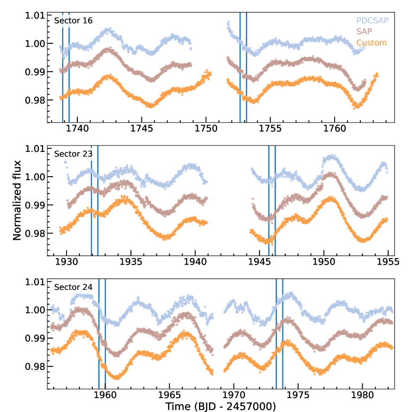
Figure 1: TESS lightcurves of Group-X candidate member TIC 159873822, aka TOI 2048. Data from PDCSAP (light blue), SAP (light brown), and our custom pipeline (orange) are shown; our custom pipeline was applied to the 2 minute cadence data in this case for ease of comparison. All data have been binned to 30 minutes and offset vertically for clarity. From top to bottom, TESS sectors 16, 23, and 24 are shown. Fluxes have been normalized, and the time is given in TBJD (BJD$-2457000$). The locations of the transits of TOI 2048b, the exoplanet we statistically validate in this work, are indicated by the vertical blue lines. The transits are evident in all three reductions but the first (near TBJD=$1739$) is effected by the systematics correction in the PDCSAP data. SAP and FFI data both double-peaked rotational modulation; this light curve has a strong signal at both our favored $P_{\star}=8$ d and at the half-period $P_{\star}/2=4$ d. In the PDCSAP data, the asymmetry in the double peaks has been partially removed by the systematics correction. There is very little signal remaining at $P_{\star}$, and rotation analysis favors $P_{\star}/2$.

2.1.2 Ground-based transit follow-up from LCOGT

We observed three transits using the Las Cumbres Observatory (LCO; Brown et al., 2013) 1m telescopes at the McDonald Observatory, Texas, USA and Teide Observatory, Canary Islands. The observations on 2020-09-05 were obtained in the Pan-STARRS $z$-short band, and those on 2021-03-03 and 2022-04-20 in Sloan $i^{\prime}$ band. The LCO BANZAI pipeline (McCully et al., 2018) was used the calibrate the data, and AstroImageJ (Collins et al., 2017) was used to extract the photometry using an aperture with radius $5\farcs 8$. No sources within this distance were identified with our AO imaging or in Gaia data (§2.4). The 2021-03-03 observation suffered from an equipment problem that resulted in the dome or camera shutter rotating into the image throughout the observation and eventually obscuring the target star.

The 2020-09-05 data do not contain sufficient out of transit baseline to constrain the timing or depth of the transit itself, but demonstrate that neighboring stars do not show clear eclipses that could be responsible for the signal associated with TOI 2048.01. The 2022-04-20 data firmly rule out NEBs in stars within 2.5 arcmin of the target over a $-2.1\sigma$ to $+2.7\sigma$ observing window relative to the TESS sector 24 QLP ephemeris. The light curves of all neighboring stars had RMS less than 0.2 times the depth required in the respective star to produce the detection in the TESS aperture. The target star light curve shows a tentative detection of a $\sim 1000$ ppm ingress arriving roughly 24 minutes ($0.5\sigma$) late relative to the nominal TESS sector 24 QLP ephemeris. Given the ingress-only coverage, we consider the timing of the apparent ingress detection tentative and do not further consider it in the analyses in this paper. The 2021-03-03 data show an apparent short, deep event; the latter part of the 2021-03-03 data were not used due to data issues. The apparent event is inconsistent with both the TESS transit and the data from 2020-09-05 and 2022-04-20, and coincides with a similar event seen on a neighboring star. We conclude that the event seen on 2021-03-03 is likely caused by the equipment problem and is not astrophysical. All ground-based follow-up light curves are available on ExoFOP.

2.2 Ground-based transit follow-up from MuSCAT2

TOI 2048 was observed on the night of 2022-04-20 with the multicolor imager MuSCAT2 (Narita et al., 2019) mounted on the 1.5 m Telescopio Carlos Sánchez (TCS) at Teide Observatory, Spain. MuSCAT2 has four CCDs with $1024\times 1024$ pixels and each camera has a field of view of $7.4\times 7.4$ arcmin² (pixel scale of 0.44 arcsec pixel^-1. The instrument is capable of taking images simultaneously in Sloan $g^{\prime}$, $r^{\prime}$, $i^{\prime}$, and $z_{s}$ bands with little (1-4 seconds) read out time.

The observations were made with the telescope slightly defocused to avoid the saturation of the target star, in the night of the transit event the $i^{\prime}$ band camera presented some connection issues and could not be used. The exposure times were initially set to 5 seconds to all the bands and then changed to 3, 3, and 2.5 seconds in $g^{\prime}$, $r^{\prime}$, and $z_{s}$ respectively to avoid saturation. The raw data were reduced by the MuSCAT2 pipeline (Parviainen et al., 2019) which performs standard image calibration, aperture photometry, and is capable of modelling the instrumental systematics present in the data while simultaneously fitting a transit model to the light curve.

The MuSCAT2 light curves show a tentative detection of the ingress on the target star with a timing and depth consistent with LCO data taken on the same night and observatory. We measured a central transit time of $T_{c}=2459690.6616\pm 0.0035$ BJD and transit depths of $\sim 1190$, $1220$, and $1560$ ppm in $g^{\prime}$, $r^{\prime}$, and $z_{s}$ respectively.

2.3 High resolution optical spectroscopy

2.3.1 FLWO/TRES

We obtained four spectra with the Tillinghast Reflector Echelle Spectrograph (TRES; Fűrész et al., 2008). TRES is on the 1.5m Tillinghast Reflector at Fred Lawrence Whipple Observatory (FLWO), Arizona, USA. TRES has a resolution of around $44000$ and covers $3900$Å to $9100$Å. The S/N of our spectra is about 25. Spectra were timed to coincide with opposite quadratures of the candidate planetary signal. The spectra were obtained between August 2020 and September 2021. The spectra were extracted as described in Buchhave et al. (2010). These data are available on ExoFOP ExoFOP (2019).²

2.3.2 McDonald/Tull

We obtained high resolution visible spectra of 33 candidate members of Group-X (including TOI 2048) with the Tull coudé spectrograph on the 2.7-m Harlan J. Smith telescope at McDonald Observatory (Tull et al., 1995). The Tull spectrograph is a cross-dispersed echelle spectrograph that covers a wavelength range from $\sim$3400–10000 Å at a resolution of roughly 60,000. 47 spectra were taken between July 2020 and May 2021, with 11 targets having multiple observations taken (to increase S/N or investigate possible binarity). Exposure times ranged from 300 s to 1500 s, chosen to achieve sufficient S/N to measure the equivalent width of the Li 6708 Å spectral feature. Spectra were reduced using a custom python implementation of standard reduction procedures. After bias subtraction, flat-field correction, and cosmic ray rejection, we extract 1D spectra from the 2D echellograms using optimal extraction. We derive wavelength solutions using a series of ThAr lamp comparison observations taken throughout each observing night. Finally, we fit the continuum using an iterative b-spline to produce flux-normalized spectra. The median S/N in the spectral order that contains the Li 6708 Å feature is 45.

We measured RVs from the Tull coudé spectra by computing spectral-line broadening functions (BFs) using the python implementation saphires (Rucinski, 1992; Tofflemire et al., 2019). The BF is computed from the deconvolution of an observed spectrum with a narrow-lined template and effectively reconstructs the average stellar absorption-line profile in velocity space. As templates, we used Phoenix spectra (Husser et al., 2013) that are matched to the stellar effective temperature estimated from the Gaia $G_{\rm BP}-G_{\rm RP}$ color. We computed BFs for the 25 spectral orders with minimal telluric contamination, covering a wavelength range from 4730–8900 Å. We fit the BFs with a Gaussian to determine the peak location and thus the RV. We correct for barycentric motion using barycorrpy (Kanodia & Wright, 2018), which implements the formalism of Wright & Eastman (2014). We then iteratively combine the RVs from the individual orders. At each iteration, we compute the mean and take the error in the mean as the uncertainty, then reject orders with RVs $>3\sigma$ from the average and recomputing the combined RV. No exposure uses fewer than 22 of the 25 orders. For the 11 objects with multiple observations, we adopt the weighted average and error as the RV and its uncertainty.

Two targets (Gaia EDR3 1601557162529801856 and Gaia EDR3 1615954442661853056) have double peaked BFs, which indicates that they are SB2s, and were each observed twice. For the former, we compute the weighted average and error for each exposure using the individually fit RV peaks to get the systemic RV, and then adopt the average systemic RV across both observations. For the latter, we adopt the RV computed from the second observation as the two SB2 components are overlapping, which should provide the systemic RV.

The RVs from our high resolution optical spectra are used as part of our Li measurements (§4.5), but are not included in our assessment of Group-X membership. They are included in Tab. 7.

2.4 AO imaging

2.4.1 Speckle polarimeter

We observed TOI-2048 on 2021 January 23 UT with the Speckle Polarimeter (Safonov et al., 2017) on the 2.5 m telescope at the Caucasian Observatory of Sternberg Astronomical Institute (SAI) of Lomonosov Moscow State University. SPP uses Electron Multiplying CCD Andor iXon 897 as a detector. The atmospheric dispersion compensator allowed observation of this relatively faint target through the wide-band $I_{c}$ filter. The power spectrum was estimated from 4000 frames with 30 ms exposure. The detector has a pixel scale of $20.6$ mas pixel^-1, and the angular resolution was 89 mas. We did not detect any stellar companions brighter than $\Delta I_{C}=4$ and $5.8$ at $\rho=0\farcs 25$ and $1\farcs 0$, respectively, where $\rho$ is the separation between the source and the potential companion.

2.4.2 Shane/ShARCS

We observed TOI 2048 on 2021 March 29 using the ShARCS camera on the Shane 3-meter telescope at Lick Observatory, California, USA (Kupke et al., 2012; Gavel et al., 2014; McGurk et al., 2014). Observations were taken with the Shane adaptive optics system in natural guide star mode. We collected two sequences of observations, one with a $Ks$ filter ($\lambda_{0}=2.150$ $\mu$m, $\Delta\lambda=0.320$ $\mu$m) and one with a $J$ filter ($\lambda_{0}=1.238$ $\mu$m, $\Delta\lambda=0.271$ $\mu$m). A more detailed description of the observing strategy and reduction procedure can be found in Savel et al. (2020). We find no nearby stellar companions within our detection limits.

2.4.3 Palomar/PHARO

We observed TOI 2048 with PHARO (Hayward et al., 2001) at Palomar Observatory, California, USA on 2021 Feb 23, behind the natural guide star AO system P3K (Dekany et al., 2013). PHARO has a pixel scale of $0.025\arcsec$ per pixel for a total field of view of $\sim 25\arcsec$. We used the narrow-band $Br\gamma$ filter $(\lambda_{o}=2.1686~{}\mu$m, $\Delta\lambda=0.0326~{}\mu$m). We used a standard 5-point dither with steps of 5″, revisiting each position with an offset of 0.5^′′ three times. The total integration time was 148 seconds.

We processed the AO data with a custom set of IDL tools that performed flat-fielding, sky subtraction, and dark subtraction. The images were combined, producing a combined image with a point spread function (PSF) full-width at half-maximum of $0.098\arcsec$. No stellar companions were found within the $5\sigma$ detection limits, as determined in injection and recovery tests.

2.4.4 Keck/NIRC2

We observed TOI 2048 and two calibrator stars (HIP 77903 and TYC 3877-725-1) on 2020 June 30 at Keck Observatory using the NIRC2 adaptive optics camera and natural guide star adaptive optics. We observed each star with standard imaging, coronagraphic imaging, and non-redundant aperture masking in the $K^{\prime}$ filter ($\lambda$ = 2.124 $\mu$m). All observations used the narrow camera, which has a pixel scale of 9.971 mas pixel^-1 (Service et al., 2016) and a field of view of 10″. For sensitivity at wide separations, we obtained some images with the partially-transmissive 0.6″-diameter coronagraph. For sensitivity to companions near and inside the diffraction limit, we also obtained interferograms using a 9-hole aperture mask placed in the re-imaged pupil plane.

All images were dark-subtracted with mode-matched dark frames, linearized, flatfielded, and screened for cosmic rays and known hot/dead pixels. Additionally, spatially coherent EM interference noise (which manifests as “stripe noise” and which otherwise dominates the faint-source flux limit) was subtracted from each quadrant using the median of the other three quadrants.

We estimated companion detection limits following the procedures of Kraus et al. (2016), To summarize, we create two residual maps tailored to identify wide-separation candidate companions amidst readnoise and scattered light, and to identify close-in candidate companions amidst speckle noise. The former is generally more sensitive at separations $\gtrsim 0.5\arcsec$. We estimated the source detection limits as a function of projected separation as the contrast that would correspond to a $+6\sigma$ outlier at any given radius.

We found no candidate detections above this limit for TOI 2048 or either calibrator, and hence no candidate companions within the NIRC2 FOV around each star ($\rho\lesssim 5\arcsec$). We summarize the NIRC2 observations and detection limits in Table 1, and plot the contrast curve in Figure 2.

Table 1: Detection Limits for Keck/NIRC2 Imaging

Name	Epoch	Filter+	$N_{obs}$	$t_{int}$	Contrast $\Delta m$ (mag) at $\rho=$ (mas)										PI
	(MJD)	Coronagraph		(sec)	150	200	250	300	400	500	700	1000	1500	2000
TYC 3877-725-1	59030.26	Kp	2	40.00	4.4	5.1	5.9	5.9	6.8	7.0	7.8	8.7	8.8	8.9	Huber
TYC 3877-725-1	59030.26	Kp+C06	4	80.00	…	…	…	…	7.5	8.0	9.2	10.3	11.2	12.1	Huber
TOI-2048	59030.27	Kp	2	40.00	5.4	5.9	6.5	6.8	7.4	7.6	8.2	8.3	8.4	8.4	Huber
TOI-2048	59030.27	Kp+C06	7	140.00	…	…	…	…	7.5	8.2	9.2	10.6	11.4	12.2	Huber
HIP 77903	59030.28	Kp	4	80.00	5.7	5.9	6.6	6.9	7.4	7.7	8.4	9.4	9.6	9.7	Huber
HIP 77903	59030.29	Kp+C06	5	100.00	…	…	…	…	7.5	8.2	9.3	10.7	11.6	12.4	Huber

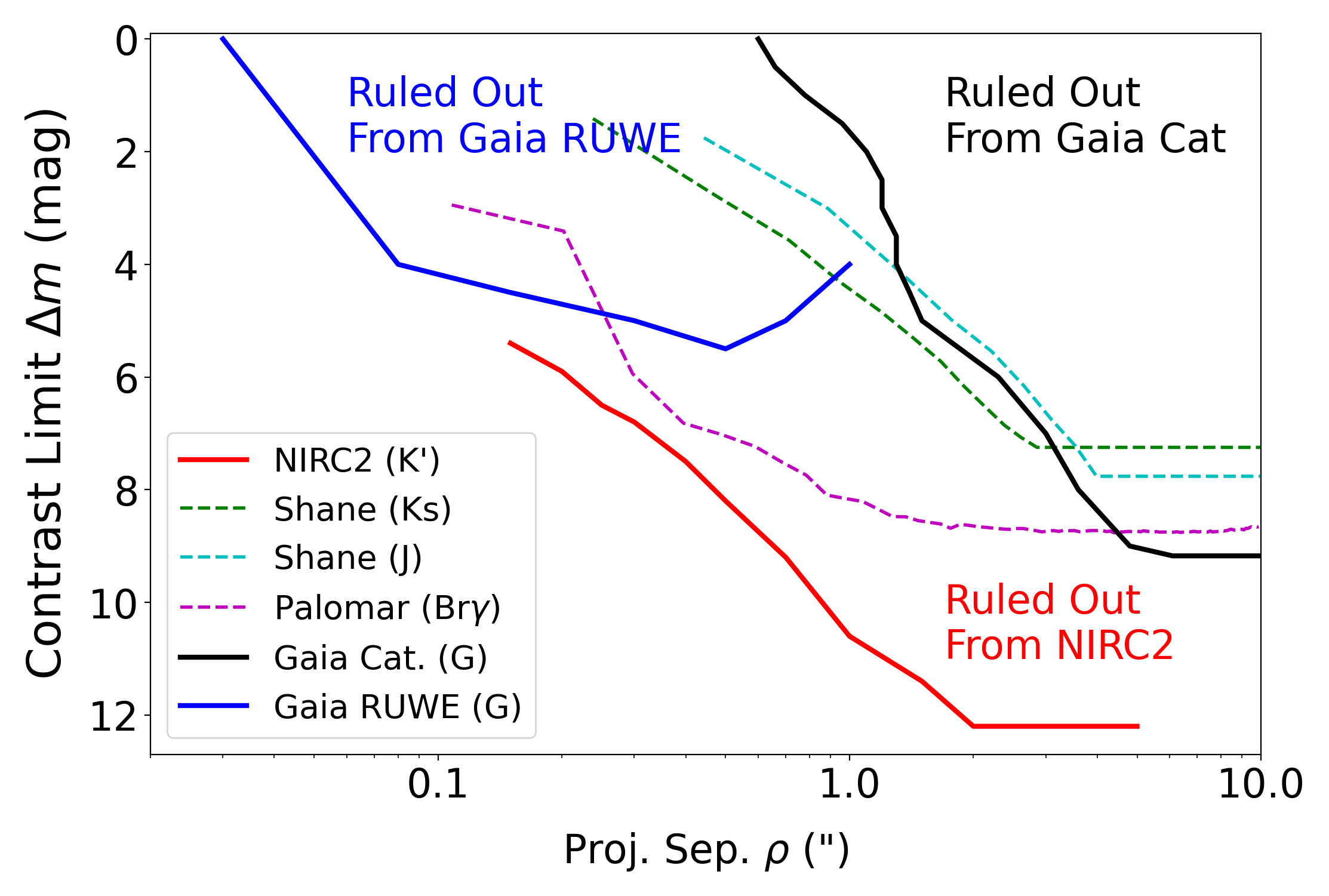
Figure 2: Contrast limits for close neighbors to TOI 2048, as found from Keck/NIRC2 AO imaging (at $K^{\prime}$ or $\lambda=2.124\mu$m; red), the absence of Gaia catalog sources (at $G$ or $\lambda=0.639\mu$m; black), and the absence of elevated astrometric noise in the RUWE (at $G$; blue). These data provide the strongest constraints and are used to statistically validate TOI 2048 b. Also shown are contrast limits from Shane (at $K_{s}$; dashed green, and $J$; dashed cyan) and Palomar (at $Br\gamma$; dashed magenta). The detection limits rule out any binary companions above the hydrogen burning limit at projected separations of $\rho\gtrsim$25 AU and equal-brightness binary companions at $\rho\gtrsim 4$ AU.

2.5 Astrometry from Gaia

The Gaia Renormalized Unit Weight Error (RUWE; Lindegren et al. 2018) is a measure of excess noise in the Gaia astrometric solution. This excess noise has been recognized as an indicator potential binarity (Lindegren et al., 2018) due to either true photocenter motion (Belokurov et al., 2020) or PSF-mismatch error in the Gaia astrometry (Kraus et al., in prep), and it is surprisingly sensitive to close companions (e.g. Rizzuto et al., 2018; Wood et al., 2021). TOI 2048 has RUWE = 0.90, which is consistent with the range of RUWE values seen for single stars in the field (Bryson et al. 2020; Kraus et al., in prep) and in young populations (Fitton et al., 2022). Based on a calibration with known field binary companions by Kraus et al. (in prep), the lack of excess RUWE indicates that there are no spatially resolved companions with equal brightness at $\rho>0.03\arcsec$, $\Delta G<4$ mag at $\rho>0.08\arcsec$, or $\Delta G<5$ mag at $\rho>0.2\arcsec$. We included this limit in Figure 2.

The Gaia EDR3 catalog (Collaboration et al., 2021) also can reveal wider comoving neighbors. Equal-brightness sources are generally recognized in the Gaia catalog down to $\sim 0.6\arcsec$, and even very faint neighbors are identified down to a few arcseconds (Ziegler et al., 2018; Brandeker & Cataldi, 2019); we also include this limit in Figure 2. At wide separations, the flux limit for the Gaia catalog is $G<20.5$ mag ($M\sim 80M_{Jup}$; Baraffe et al. 2015). The Gaia catalog contains no sources within $\rho<44\arcsec$ ($\rho<5000$ AU).

The nearest source with a marginally consistent parallax and proper motion (Gaia EDR3 1404652153462037248) has a projected angular separation of $\rho=1700\arcsec$ ($\rho\sim 1$ pc). However, the parallactic distance even for that source differs by $\Delta D=7.9\pm 0.8$ pc (a $10~{}\sigma$ difference), so it is most likely an unbound sibling within Group-X.

We concluded that there are no wide binary companions to TOI 2048 above the substellar boundary. We use the limits from RUWE and the Gaia source catalog to supplement NIRC2 imagining constraints on companions in our false positive analyses (§5.2.2).

2.6 Literature photometry

We used optical and near-infrared (NIR) photometry from a variety of sources in our fit to the spectral energy distribution. We used optical photometry from Gaia EDR3 (Gaia Collaboration et al., 2021, 2018), the AAVSO All-Sky Photometric Survey (APASS, Henden et al., 2012), Tycho-2 (Høg et al., 2000), and the Sloan Digital Sky Survey thirteenth data release (SDSS DR13; Albareti et al., 2017). We used NIR photometry from the Two-Micron All-Sky Survey (2MASS, Skrutskie et al., 2006) and the Wide-field Infrared Survey Explorer (WISE, Wright et al., 2010).

3 Analysis of host star TOI 2048

3.1 Stellar parameters

Table 2: Properties of the host star TOI 2048.

Parameter	Value	Source
Identifiers
TOI	2048
TIC	159873822
TYC	3496-1082-1
2MASS	J15514181$+$5218226
Gaia DR2	1404488390652463872
Astrometry
$\alpha$	15:51:41.79	Gaia EDR3
$\delta$	52:18:22.71	Gaia EDR3
$\mu_{\alpha}$ (mas yr-1)	$-10.255\pm 0.013$	Gaia EDR3
$\mu_{\delta}$ (mas yr-1)	$-1.404\pm 0.015$	Gaia EDR3
$\pi$ (mas)	$8.592\pm 0.012$ Gaia EDR3
Photometry
$G_{\mathrm{Gaia}}$	$11.3252\pm 0.0009$	Gaia DR2
$BP_{\mathrm{Gaia}}$	$11.817\pm 0.003$	Gaia DR2
$RP_{\mathrm{Gaia}}$	$10.704\pm 0.002$	Gaia DR2
$J$	$9.89\pm 0.02$	2MASS
$H$	$9.54\pm 0.01$	2MASS
$K$	$9.44\pm 0.01$	2MASS
$B_{T}$	$12.6\pm 0.2$	Tycho-2
$V_{T}$	$11.5\pm 0.1$	Tycho-2
$B$	$12.54\pm 0.05$	APASS
$V$	$11.53\pm 0.05$	APASS
$W1$	$9.38\pm 0.02$	ALLWISE
$W2$	$9.43\pm 0.02$	ALLWISE
$W3$	$9.34\pm 0.03$	ALLWISE
$W4$	$9.2\pm 0.3$	ALLWISE
$g$	$12.11\pm 0.03$	SDSS
$r$	$11.35\pm 0.03$	SDSS
$i$	$11.12\pm 0.03$	SDSS
$z$	$11.51\pm 0.03$	SDSS
Kinematics & Position
Barycentric RV (km  s-1)	$-7.6\pm 0.1$	This paper
Distance (pc)	$116.39\pm 0.17$	From parallax
U (km  s-1)a	$-2.3$	This paper
V (km  s-1)a	$-9.0$	This paper
W (km  s-1)a	$-1.9$	This paper
X (pc)	$10.2$	This paper
Y (pc)	$76.9$	This paper
Z (pc)	$86.7$	This paper
Physical Properties
Rotation Period (days)	$7.97^{+0.08}_{-0.19}$	This paper
$v\sin{i_{\star}}$(km  s-1)	$4.8\pm 0.7$ $\rm km~{}s^{-1}$	This paper
$i_{\star}$ (∘)	$i=71_{-14}^{+12}$	This paperb
$F_{\mathrm{bol}}$ (erg cm-2 s-1)	$(9.64\pm 0.022)\times 10^{-10}$	This paper
$R_{\star}$ ($R_{\odot}$)	$0.79\pm 0.04$	This paper
$M_{\star}$ ($M_{\odot}$)	$0.83\pm 0.03$	This paper
$L_{\star}$ ($L_{\odot}$)	$0.41\pm 0.04$	This paper
$T_{\text{eff}}$	$5185\pm 60$	This paper
$E(B-V)$ (mag)	$0.11\pm 0.07$	This paper
[m/H]	$0.02\pm 0.08$	This paperc
Age (Myr)	$300\pm 50$	This paperd

Note. — ^aNot corrected for the local standard of rest. ^b $i_{\star}$ adopts the convention $i_{\star}<90\degree$. ^cDetermined from TRES spectra using SPC. ^dBased on gyrochronology (§4.3), we adopt the age of NGC 3532 (Fritzewski et al., 2019) as the age of Group-X.

We summarize the stellar properties deriving from our analysis in Table 2.

3.1.1 Fit to the spectral energy distribution

We fit the spectral-energy distribution by comparing spectral templates to the observed photometry, following the method detailed in Mann et al. (2016a). The templates cover 0.4–2.3$\mu$m, with gaps in regions of high telluric contamination (primarily H₂O bands in the NIR). To fill these gaps and extend the spectrum past the limits, we included BT-SETTL CIFIST atmospheric models (Baraffe et al., 2015) in the fit, which also provided an estimate of $T_{\text{eff}}$. To estimate the bolometric flux ($F_{\mathrm{bol}}$), we took the integral of the resulting absolutely-calibrated spectrum. We combined $F_{\mathrm{bol}}$ with the Gaia parallax to determine the total stellar luminosity ($L_{\star}$). With $T_{\text{eff}}$ and $L_{\star}$, we calculated $R_{\star}$ from the Stefan-Boltzmann relation. Reddening is expected to be small but potentially non-zero for a star at this distance, so we include extinction as part of the fit. To account for variability in the star, we added (in quadrature) 0.02 mags to the errors of all optical photometry. The resulting fit included six free parameters: the spectral template, $A_{V}$, three BT-SETTL model parameters ($\log~{}g$, $T_{\text{eff}}$, and [M/H]), and a scaling factor that matches the model to the photometry. This scale factor is equivalent to $(R_{\star}/D)^{2}$, which provides a separate estimate of $R_{\star}$ based on the infrared-flux method (IRFM; Blackwell & Shallis, 1977). We show an example fit in Figure 3.

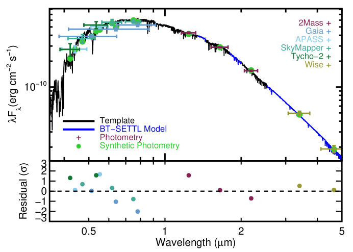
Figure 3: Example fit from our SED analysis. The black line indicates the template spectrum (a G8V) and the blue shows the BT-SETTL models used to fill in gaps. Synthetic photometry from the template and model is shown in green. Observed photometry is colored based on the source, with vertical errors corresponding to the measurement errors and horizontal errors the filter width. The bottom panel shows the fit residual in units of standard deviations.

The resulting fit yielded $E(B-V)=0.11\pm 0.07$, $T_{\text{eff}}$ $=5185\pm 60$ K, $F_{\mathrm{bol}}$ $=(9.64\pm 0.022)\times 10^{-10}$ (erg cm^-2 s^-1), $L_{\star}=0.41\pm 0.04L_{\odot}$, and $R_{\star}=0.79\pm 0.04R_{\odot}$. The errors account for uncertainty due to template choice, measurement uncertainties in the photometry and parallax, and uncertainties in the filter zero-points and profiles (Mann & von Braun, 2015). The IRFM fit gave a radius of $0.75\pm 0.02R_{\odot}$, consistent with the value from the Stefan-Boltzmann relation. We adopt the former as the more conservative radius for our analysis.

The TRES spectra were also used to derive stellar parameters using the Stellar Parameter Classification tool (SPC Buchhave et al., 2010). SPC cross correlates an observed spectrum against a grid of synthetic spectra based on the Kurucz atmospheric model (Kurucz, 1992). SPC values were consistent with those derived above, and additionally indicate near-solar metallicity ([m/H] $=0.02\pm 0.08$).

3.1.2 Mass from evolutionary models

To determine $M_{\star}$ we interpolated the observed photometry onto a grid of solar-metallicity models from the Dartmouth Stellar Evolution Program (DSEP; Dotter et al., 2008). We fit for age, $A_{V}$, and $M_{\star}$ within an MCMC framework. An additional parameter ($f$, in magnitudes) captured underestimated uncertainties in the data or models. For computational efficiency, we used a two-step interpolator to find the nearest age in the model grid and then performed linear interpolation in mass to obtain stellar parameters and synthetic photometry. This nearest-age approach can generate errors from the grid spacing, so we pre-interpolated the grid in age and mass using the isochrones package (Morton, 2015). This also let us use a grid uniform in age. To redden model photometry, we used synphot (Lim, 2020). We applied Gaussian priors on age ($300\pm 50$ Myr, based on the rotation analysis in §4.3) and $T_{\text{eff}}$ (5185$\pm$60 K, based on our SED fit). Other parameters had uniform priors.

This analysis yielded $M_{\star}=0.844\pm 0.017M_{\odot}$ and $R_{\star}=0.742\pm 0.011R_{\odot}$. Repeating the analysis with the PARSEC isochrones (Bressan et al., 2012; Chen et al., 2015) yielded a mass of $M_{\star}=0.824\pm 0.013M_{\odot}$ and $R_{\star}=0.735\pm 0.009R_{\odot}$. The values are consistent with those derived using DSEP models and both radii are consistent with our SED fit. The errors were likely underestimated, however, as model systematics dominate and we did not account for effects of metallicity or activity. For the mass, we adopted $M_{\star}=0.83\pm 0.03M_{\odot}$ with the larger errors more reflective of model disagreements seen in young eclipsing binaries (e.g., David et al., 2016; Kraus et al., 2017). We adopted the more empirical $R_{\star}$ from the previous section.

3.2 Velocities

We measured relative velocities using a multi-order analysis (Buchhave et al., 2010). Using the highest S/N spectrum as a template, we cross-correlated against the remaining spectra, order by order. We then co-added the cross-correlation functions, which has the effect of weighting by flux. This analysis did not show large velocity variations that would be expected if there were a stellar companion. These values are listed in Table 3.

To measure absolute velocities, we compared our observed spectra to a synthetic template to compute the BF (see §2.3.2). We then fit the BF with a Gaussian to measure the radial velocity. This was done independently for each order, and we took the standard deviation of the order-by-order measurements as the error. We then adopt the weighted mean and standard deviation of the velocity measurements from each spectrum as the final radial velocity. Based on the first three TRES spectra, the absolute RV is $-7.6\pm 0.1$$\rm km~{}s^{-1}$. Although the Gaia DR2 velocities do not have a published epoch or an established zeropoint, the value for TOI 2048 of $-7.4\pm 0.6$ $\rm km~{}s^{-1}$ is in good agreement with our TRES measurements.

Table 3: TOI 2048 relative radial velocity measurements

Site	BJD	RV	$\sigma_{RV}$	S/N
		(m s-1)	(m s-1)
TRES	2459038.772371	$-$190.46	33.56	28
TRES	2459059.798755	$-$84.46	48.81	20
TRES	2459232.050855	$-$35.97	32.42	25
TRES	2459472.628102	0.00	33.56	31

3.3 Stellar rotation

3.3.1 Rotation period

We modeled the stellar rotation signal in the TESS photometry using Gaussian processes. As discussed in §2.1.1, we used the SAP light curve data for this analysis. We masked the transits using a preliminary transit fit before proceeding.

We used the exoplanet package (Foreman-Mackey et al., 2021) for our model and pymc3 (Salvatier et al., 2016) for optimization. The stellar rotation capabilities for exoplanet are built on the Gaussian Process package celerite2 (Foreman-Mackey et al., 2017; Foreman-Mackey, 2018). We set up the model with a non-periodic component to describe trends in the data, and a quasi-periodic component to describe the stellar rotation signal.

The quasi-periodic term is a mixture of two damped simple harmonic oscillators at $P_{\star}$ and $P_{\star}/2$. This mixture is characterized by the rotation period ($P_{\star}$, sampled as $\log{P_{\star}}$), the amplitudes of two oscillators, and the quality factors of the two oscillators that characterized how damped they are. The amplitudes are characterized by the amplitude of the signal at $P_{\star}$ ($\sigma$, sampled as $\log\sigma$), and the fractional amplitude of the signal at $P_{\star}/2$ ($f$, such that the amplitude is $f\sigma$). The quality factors are characterized by the quality factor $Q$ of signal at $P_{\star}/2$ ($Q$, such that the quality factor is $Q_{2}=1/2+Q$, and the difference in the quality factors between the signals ($\delta Q$, such that $Q_{1}=1/2+Q+\delta Q$). These were sampled as $\log{Q}$ and $\log{\delta Q}$. Priors are listed in Table 4.

Table 4: Stellar rotation modeling priors and fits.

Parameter	Prior			Fitted Value
	$\mu$	$\sigma$	limits
$\log{P_{\star}/d}$	8	1	$\cdots$	$2.076^{+0.010}_{-0.025}$
$\log{a}$	$\cdots$	$\cdots$	[$-20$,$5$]	$1.29^{+0.18}_{-0.13}$
$f$	$\cdots$	$\cdots$	[0,1]	$0.65^{+0.22}_{-0.26}$
$\log{Q_{0}}$	0	5	$\cdots$	$1.3^{+0.44}_{-0.39}$
$\log{\Delta Q}$	0	5	$\cdots$	$2.7^{+3.2}_{-3.6}$
$\mu_{\mathrm{flux}}$ (ppt)	0	0.5	$\cdots$	$0.17\pm 0.19$

Note. — Parameters that use Gaussian priors list the mean ($\mu$) and standard deviation $\sigma$, while those that use uniform priors list the limits. The best-fitting values are the median and 68% confidence intervals of the posterior distribution.

We first fit the data using maximum likelihood, and clipped 5$\sigma$ outliers from the model (with the standard deviation calculated as 1.48 times the median absolute deviation). We then re-fit the data using Markov Chain Monte Carlo (MCMC). We used 4000 tuning steps, 4000 draws, and ran six chains. The Gelman-Rubin statistic ($\hat{R}$) was $1.0$ for all parameters, and there were no divergences in the chains after tuning (which would indicate regions of parameter space that may not have effectively been explored), indicating that the MCMC converged.

Figure 4 shows our fit to the data for TESS sectors 23 and 24. Table 4 includes our best fit values and errors. We measure a stellar rotation period of $7.97^{+0.08}_{-0.19}$ days.

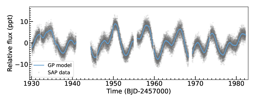
Figure 4: TESS-SPOC data (grey points) and Gaussian Process stellar variability model (blue curve). Time is given in TJBD and the flux units are parts per thousand (ppt). The transits of TOI 2048 b were removed before fitting and are not shown; outliers from the preliminary fit are also not shown.

3.3.2 Rotational broadening

We measure the projected rotational velocity ($v\sin{i_{\star}}$) from the first three TRES spectra by fitting the co-added BFs from each epoch with a broadened absorption-line model (Gray, 2008). The model is broadened by the TRES spectral resolution, rotational broadening, and macroturbulent velocity ($v_{mac}$). The computed BF profile is not sufficiently broad with respect to the TRES instrumental resolution to independently constrain the rotational and $v_{mac}$ broadening components. As such, we estimate $v_{mac}$ using the $T_{\text{eff}}$ and $\log{g}$  dependent relation derived by Doyle et al. (2014). For TOI 2048, this corresponds to 2.3 $\rm km~{}s^{-1}$. Adopting this value, we fit an average $v\sin{i_{\star}}$ value of 4.8 $\rm km~{}s^{-1}$ from the three epochs. Adding the standard deviation of our $v\sin{i_{\star}}$ measurements with the uncertainty of the $v_{mac}$ relation in quadrature, we determine and uncertainty of 0.7 $\rm km~{}s^{-1}$.

The Doyle et al. (2014) $v_{mac}$ relation is derived using a sample of field-age stars, and there may be an age dependence missing in the relationship that we have not accounted for. To validate our adopted value $v_{mac}$ above, we perform the same measurement on the single Tull coudé spectrum we obtained (Section 2.3.2), finding a consistent $v\sin{i_{\star}}$ value. Due to the difference in their spectral resolutions, obtaining a consistent $v\sin{i_{\star}}$ measurement between these instruments provides independent confirmation that the adopted $v_{mac}$ value is appropriate for TOI 2048.

3.3.3 Inclination

We used the photometric rotation period, stellar radius, and $v\sin{i}$ to measure the inclination of the stellar spin axis to the line-of-sight. We sampled the posterior of $\cos{i}_{*}$ as in Newton et al. (2019), following the formalism from Masuda & Winn (2020) and using the Goodman & Weare (2010) affine invariant MCMC sampler. We used the values and errors in Table 2 to set Gaussian priors on all parameters, and imposed $0\leqslant\cos{i}_{*}\leqslant 1$. We took the median and 68% confidence intervals of the $\cos{i}_{*}$ posterior as the best value and error. Under the convention that $i_{\star}<90^{\circ}$, $i=71_{-14}^{+12}$. This is suggestive that the stellar rotation and the planetary orbital axes are misaligned; however, the uncertainties are large and the $2\sigma$ confidence interval extends to $89^{\circ}$.

4 Analysis of Group-X candidate members

4.1 Identification of candidate cluster members

We adopted the union of two catalogs as the final candidate member list of Group-X. Tang et al. (2019) identified 218 candidates, and Fürnkranz et al. (2019) 177, from clustering analyses of Gaia DR2 sources in 5D (position and proper motion) space. We supplemented this list in the vicinity of TOI 2048 using the FindFriends routine (Tofflemire et al., 2021). We queried Gaia EDR3 within a 25 pc volume and identified all candidates which had reprojected tangential velocities relative to TOI 2048 $\Delta v_{tan}<5$ $\rm km~{}s^{-1}$. We found 208 candidates which we refer to as Friends. The Friends include 69 stars in common with the Tang et al. catalog. These stars are listed in Table 5.

Table 5: Combined Group-X members

Gaia EDR3 ID	TIC ID	R.A.	Dec.	PMRA	PMDEC	Tang?	Fürnkranz?	Friend?
		degrees	degrees	mas yr-1	mas yr-1
4034556767349900032	365967521	178.9487619378884	39.07336135237724	-20.852769509956776	-9.705086459861777	True	False	False
1536085299544341888	21573379	181.613103458542	40.05711606627952	-17.601822134658658	-9.850233966424518	True	False	False
1532033908433815552	376690520	187.79913230841564	38.78275454051492	-16.12143949882819	-2.211138299093715	True	False	False
1568098405222585600	157878723	191.7620198027893	50.57455869427148	-19.639383362412357	-8.543337791170309	True	False	False
1555402481895361664	334518873	193.69320930034883	49.16955179153733	-20.64025984104685	-8.50133287045549	True	False	False

Note. — This table is included in its entirety online as a machine readable table.

The sky positions and proper motions of both lists are shown in Figure 5. The original Group-X candidate members from Tang et al. and Fürnkranz et al. (2019) are part of an elongated group, with TOI 2048 sitting in the outskirts (TOI 2048 is not included as a member by Fürnkranz et al.). By design, the TOI 2048 Friends are located in a region centered on TOI 2048. Stars most closely matching TOI 2048 in proper motion are most likely to be part of the elongated structure identified as Group-X (see Figure 5). Our Friends analysis indicates that the phase-space region around TOI 2048 is more populated than originally suggested, resulting in an even more elongated structure for Group-X. A detailed membership analysis is warranted, but as a first pass we draw a distinction at Friends with $\Delta v_{tan}=2$ $\rm km~{}s^{-1}$ based on visual inspection of Figure 5: Friends with $\Delta v_{tan}<2$ $\rm km~{}s^{-1}$ are likely members of Group-X.

We matched sources in our Friends catalog to the TESS Input Catalog (TIC; Stassun et al., 2018) based on position, with a $10\arcsec$ search radius, selecting the closest source. We matched sources in the Tang et al. catalog to the TIC using the Gaia DR2 IDs, and to Gaia EDR3 using position. We cross-matched the conjoined catalog to the TYCHO-2 catalog (Høg et al., 2000) and to the APASS 9^th data release (Henden et al., 2015) to obtain $B$ and $V$ photometry; for these two searches, we used astroquery’s XMatch routine (Ginsburg et al., 2019) with a $5\arcsec$ search radius, with the closest source being accepted.

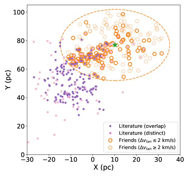
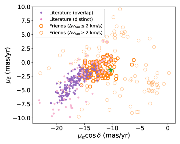
Figure 5: Galactic positions (top) and proper motions (bottom) of candidate Group-X members from Tang et al. and Fürnkranz et al. (filled pink and purple circles; pink if the star appears in only one source and purple if it appears in both), and Friends of TOI 2048 (open orange circles). TOI 2048 is marked with a green star, falling near the extremes of the association. Friends of TOI 2048 with velocity offsets $<2$ km s^-1 are the thick orange circles, those with larger velocity offsets (up to the threshhold of $5$ km s^-1) are thin orange circles. The green star marks TOI 2048; TOI 2048 is included in the candidate members list from Tang et al. (2019) but not that from Fürnkranz et al. (2019). In the position plot, the dashed circle shows the 25 pc search radius we used for FindFriends.

4.2 The color–magnitude diagram

In Figure 6, we plot candidate cluster members on a color–absolute magnitude diagram after de-redenning the magnitudes and applying quality cuts. We denote stars with $RUWE>1.3$. Extinction is minimal (the median extinction correction for stars in our sample is zero), but we calculated reddening for each source using Bayestar19 (Green et al., 2019), translated to $A_{V}$ using the provided relation, and then calculated extinction in the Gaia bandpasses using the relations provided as part of Gaia EDR3. We required S/N $>10$ for parallax S/N and $>5$ for $G$, $G_{\mathrm{BP}}$, and $G_{\mathrm{RP}}$ fluxes; and require that the corrected $G_{\mathrm{BP}}$ and $G_{\mathrm{RP}}$ flux excess factor ($C^{*}$) by $<0.04$. We calculated $C^{*}$ from phot_bp_rp_excess_factor following Riello et al. (2021, Table 2 and Equation 6).

Six stars stand out on the CMD: three stars that lie well above the main sequence and are potentially evolved, and three white dwarfs. The three evolved stars are: TIC 224312054 (Gaia EDR3 1597757387783227008), TIC 405559623 (Gaia EDR3 1602089772833227264), and TIC 166089535 (Gaia EDR3 1668291333582959232). The former two are Friends, and although both have radial velocities within $1$ $\rm km~{}s^{-1}$ of expectations for the clusters, they are also outliers in proper motion ($\Delta v_{tan}=4.8$ and $3.7$ $\rm km~{}s^{-1}$, respectively); they are unlikely to be members. None of the three’s CMD position matches evolutionary tracks for this age range.

The three white dwarfs are: TIC 1201175811 (Gaia EDR3 1622700010922131200), TIC 1200926232 (Gaia EDR3 1386173761045582336), TIC 1271282952 (Gaia EDR3 1648892576918800128). The former two are friends, with $\Delta v_{tan}=2$ and $4.7$ $\rm km~{}s^{-1}$, respectively. The latter is from Tang et al. (2019). We performed a preliminary check on the ages using wdwarfdate (Kiman 2021, Kiman et al. in prep), determining temperatures from SDSS photometry. This indicated that TIC 1201175811 and TIC 1271282952 are too old to be cluster members. TIC 1200926232 may be young (cooling age of about $370$ Myr is possible), but spectral characterization is needed. It also has RUWE $=1.3$ and may therefore be a binary.

Figure 6 includes PARSEC v1.2S isochrones (Bressan et al., 2012; Chen et al., 2015) for Gaia EDR3 colors; bolometric corrections make use of work from Chen et al. (2019) and Bohlin et al. (2020). The $300$ to $400$ Myr isochrones provided the best fit to the data; the lack of evolved stars means that the color-magnitude diagram did not provide a precise constraint on the age.

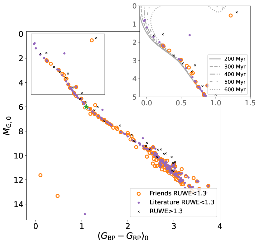
Figure 6: Absolute magnitude versus color for candidate members from Tang et al. and Fürnkranz et al. (filled purple circles) and for Friends of TOI 2048 (open orange circles). Stars with RUWE $>1.3$, indicating likely binarity, are shown as black Xs; as expected, these stars tend to lie above the main sequence. TOI 2048 is marked with the green star. The inset includes PARSEC isochrones (blue lines); the $200-400$ Myr isochrones are consistent with the cluster. The magnitudes of the stars in Group-X have been corrected for extinction (although this is insignificant), the models have not. The white dwarfs and giants are discussed in Section 4.2.

4.3 Rotation periods

We measured rotation periods independently from TESS and ZTF data. ZTF provides access to fainter stars and higher spatial resolution, but saturates on bright stars. Using TESS data, we flagged both secure and candidate detections. Secure periods were identified by eye using the criteria that 1) the peak must be clearly visible in the periodogram and 2) the lightcurve, when phase-folded on the candidate period, must look like a quasi-periodic, repeating signal. Periods detected in ZTF were considered secure.

Our combined list of stars with rotation periods includes 164 candidate Group-X members. This includes TOI 2048, for which the periodogram-based analysis of the TESS data yielded $8.1$ days, in agreement with the $7.97^{+0.08}_{-0.19}$ we measure from the same data using GPs. Rotation periods are listed in Table 6. This table does not include stars where we rejected the period. We noted five stars as having multiple signals in the periodogram; all were also flagged by either the RUWE or TESS contamination ratio cuts we applied during our analysis so we did not reject these periods.

Table 6: Rotation periods for Group-X members

TIC ID	$T_{\mathrm{mag}}$	TESS Contam. ratio	Gaia RUWE	$\Delta v_{\mathrm{tan}}$	$G_{\rm BP}-G_{\rm RP}$	TESS detection?	TESS note	ZTF detection?	$P_{\star}$
	mag			$\rm km~{}s^{-1}$	mag				d
141861147	5.738	0.0	0.83	$\cdots$	-0.037	True	y	False	1.4
459221499	7.3043	0.0	1.40	$\cdots$	0.394	True	m	False	0.33
159631183	7.77659	0.0	1.00	$\cdots$	0.467	True	y	False	0.89
166089535	6.79823	0.0	0.91	$\cdots$	0.623	True	m	False	1.6
159871715	8.5823	4.88	1.42	0.794,	.652	True	y	False	0.81

Note. — This table is included in its entirety online as a machine readable table.

4.3.1 From TESS data

We used periodograms to identify rotation periods in every star from the Friends, Tang et al. (2019), or Fürnkranz et al. (2019) lists with TESS SAP or FFI pipeline data. We used the Lomb–Scargle periodogram (Lomb, 1976; Scargle, 1982) from astropy (The Astropy Collaboration et al., 2018) as implemented in starspot. We considered rotation periods out to a maximum of 18 days and selected the highest peak in the periodogram as the candidate period. Some light curves still displayed significant long-term trends. We did not remove these systematics; however, if the highest peak in the periodogram is a result of the long-term trend and a clear candidate signal is seen in the periodogram at a shorter period, we adjusted the maximum period searched to zero-in on the candidate signal. Additionally, TIC 229668649’s periodogram peaked just beyond 18 days and we extended the search to 20 days for this star. Based on visual inspection of the periodogram, the light curve, the phased light curve, as well as the auto-correlation function, we identified stars with photometric modulation.

As discussed in §2.1.1, the PDCSAP pipeline impacts a subset of the stellar rotation signals seen in the stars we analyzed, motivating our use of SAP data over PDCSAP data. The majority of stars with periods above 6 days ($G_{\rm BP}-G_{\rm RP}>1$) were affected by this systematic, such that when using PDCSAP data there were two apparent gyrochrone sequences for the cluster with a break at $G_{\rm BP}-G_{\rm RP}\sim 1$. Using rotation periods derived from SAP data or our FFI data, the Group-X candidate members follow a single gyrochrone.

Using TESS data and without the quality checks described below, we detect periods in 133 stars and candidate periods in an additional 30. We also detected two eclipsing binaries (TIC 441702640 and TIC 165407465) and a star with $\delta$ Scuti pulsations (TIC 137834492; §4.7). Rotation period detection with TESS fell off significantly for $T>14$; since the Friends include a significant number of stars fainter than this, the following discussion is limited to brighter stars.

We detected secure periods in the TESS data alone for $61\pm 9\%$ of Friends, $70\pm 8\%$ of Tang et al. candidate members, and $68\pm 9\%$ of Fürnkranz et al. candidate members. In comparison, the fraction of stars with detected rotation periods of $P_{rot}<18$ d in the Kepler field – which we generally expect to have better sensitivity, especially to longer periods – is 14% McQuillan et al. (2014) or 16% Santos et al. (2021).

Considering the Friends, we saw a strong trend in period detection as a function of tangential velocity offset: the detection rate in Friends with $\Delta v_{tan}<2$ $\rm km~{}s^{-1}$ was $77\pm 13\%$ and drops off to $42\pm 10\%$ at larger $\Delta v_{tan}$. This is expected because TOI 2048 lies at one extreme of Group-X. A one-third detection rate is still higher than one would expect for a field population, and the detection rate did not continue to fall off at the largest $\Delta v_{tan}$, where stars are less likely to be members. We identified a small co-eval association distinct from, but nearby to, Group-X, that is contributing to period detections at larger $\Delta v_{tan}$. We call this association MELANGE-2, and we discuss it further in Appendix A.

The $21^{\prime\prime}$ pixel size means multiple Group X members occasionally fall on the same pixel. We searched for neighboring members that are relatively bright ($G_{\rm neighbor}<G_{\rm target}+1$) and within two TESS pixels and flagged them and the neighbors as blended. We then inspected each blend case: (a) when the stars were similar in color and brightness, we rejected the period for both stars, (b) when the brighter star is an A or early-F star and the fainter star is solar-type, we rejected the period for the early-type star and assigned it to the solar-type star, and finally (c) when the brighter star is solar-type and significantly brighter than the other, we rejected the period for the fainter star and assigned it to the brighter solar-type star.

4.3.2 From ZTF data

We also measured rotation periods using data from the Zwicky Transient Facility (ZTF; Bellm et al., 2019a, b). Following the Curtis et al. (2020) procedure developed for archival Palomar Transient Factory data, we downloaded 8${}^{\prime}\times$8^′ ZTF-$r$ band image cutouts from the NASA/IPAC Infrared Science Archive (IRSA), and used 6^′′ circular aperture photometry to extract light curves for each target and a selection of nearby reference stars, which are used to refine the target light curves. Rotation periods were determined using a similar Lomb–Scargle approach as was applied to the TESS data, except that the maximum period searched was set to 100 days (possible given ZTF’s longer seasonal baseline). In all, we measured periods for 78 stars from ZTF data. Of these, 68 have periods or candidate periods also measured from TESS, and the periods agreed for all but five stars; in these cases, the discrepancies were due to multiple period being detected in TESS or because the stars are EBs. Checking TESS periods with ZTF is important because the short 27-day baseline for a single TESS sector, with a large midsector data gap, makes those light curves susceptible to half-period harmonic detection, especially as periods exceed 10 days. The remaining ZTF rotators missed by TESS are typically fainter and/or more slowly rotating.

Periods for stars measured only from TESS (88 stars) or ZTF (18 stars) were adopted as the final period. We merged the TESS and ZTF periods by averaging stars with periods from both surveys that agreed to within 15%. In the few conflicting cases, we reviewed the light curves for all TESS sectors and ZTF seasons and decided what the most likely period was (e.g., when one survey found 1/2 the period of the other, we opted for the double period because the 1/2 period case is often caused by a temporary symmetric distribution of starspots around the stellar surface).

4.4 Rotation-based age

Figure 7 plots stellar rotation period as a function of color for Group-X candidate members, in comparison to stars from Praesepe and the Pleiades. Data from Praesepe were taken from Rampalli et al. (2021), and data from the Pleiades were taken from Curtis et al. (2020) with the rotation periods originating from Rebull et al. (2016). Colors have been extinction-corrected using the values from Curtis et al. (2020). Stars with TESS contamination ratios $>0.2$, RUWE $>1.3$, or $C^{*}>0.04$ (see §4.2) were not analyzed, and are not included in figures. Group-X candidate members form a clear gyrochronological sequence that lies in between Pleiades (120 Myr) and Praesepe (670 Myr) in age. A few stars, in particular several of the Friends with $\Delta v_{tan}>2$ $\rm km~{}s^{-1}$ lie along the Praesepe sequence; see Appendix A for further discussion.

Though historically there has been a gap in age between Pleiades and Praesepe for well-studied clusters, recent work on NGC 3532 enables its use as a new benchmark (Clem et al., 2011; Fritzewski et al., 2019). Fritzewski et al. (2019) provided a new membership catalog based on radial velocities, and suggest an age of $300\pm 50$ Myr based on isochrones (unlike Group-X, NGC 3532 includes several evolved stars). Fritzewski et al. (2021) measured rotation periods for NGC 3532 members, resulting in a rich, empirical gyrochrone at $300$ Myr.

Comparing stellar rotation for Group-X to NGC 3532 (Figure 7), it is clear that the two clusters have the same gyrochronological age within the uncertainties of current calibrations. While a differential gyrochronological age could be calculated (e.g. Douglas et al., 2019), the lack of calibrated gyrochronology relations at this age poses a challenge for this detailed calculation (see for example the comparison between gyrochronology relations and NGC 3532 in Figure 8 in Fritzewski et al. 2021).

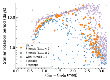
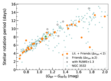
Figure 7: Rotation period versus Gaia $G_{BP}-G_{RP}$ color for stars in Group-X and comparison clusters. All colors have been corrected for reddening. Group-X candidate members from Tang et al. and Fürnkranz et al., and Friends of TOI 2048 with $\Delta v_{tan}<2$ $\rm km~{}s^{-1}$ are shown as large, filled orange circles. Unfilled orange circles are Friends with $\Delta v_{tan}>2$ $\rm km~{}s^{-1}$. TOI 2048 is the green star. In the right plot, Group-X is compared to Pleiades (blue circles; Rebull et al. 2016) and Praesepe (purple circles; Rampalli et al. 2021). The Group-X color-rotation sequence lies above the Pleiades and below the Hyades. On the left, Group-X stars are compared to NGC 3532; there is excellent agreement between the Group-X color-rotation sequence and that of NGC 3532.

During preparation of this manuscript, Messina et al. (2022) published an independent gyrochonology analysis of Group-X. They used their own reduction of TESS 30-minute cadence full-frame image data and measured rotation periods for 168 stars out of the 218 candidate members from Tang et al. (2019). Using gyrochronology relations, they determined an age of $300\pm 60$ Myr for Group-X, consistent with our conclusion.

4.5 Lithium equivalent widths

We used the spectra of Group-X candidate members obtained with the Tull Spectrograph to measure Li equivalenth widths (EWs). We discard spectra from 9 of the stars that were suspected binaries, had poor S/N ($\leq 20$, the average was $45$), or had significant fringing.

We first applied the RV and barycentric corrections derived as described in §2.3.2. We then fit a Gaussian to the Li feature at 6707.8 Å, which comprises the Li doublet and and the neighboring Iron line at 6707.4 Å, using scipy.optimize. Given the S/N of our data separating these features was not possible to deconvolve. We integrated under the curve to obtain the EW and used standard error propagation to determine the error. We constrained the line center to deviate from 6707.8 Å by no more than $0.1$ Å, a limit determined from the wavelength solution and RV errors. For stars without Li, we set the EW upper limit to $20$ mÅ. We chose this limit based on Gaussian fits we made to regions largely free of spectral features, and previous experience with data of this type.

Of the 23 stars analyzed, we measured EWs and their respective uncertainties for 13 stars, of which 11 are Friends with tangential velocity offsets $\Delta v_{tan}<2$ $\rm km~{}s^{-1}$ or are candidate members from Tang et al. (2019). The remaining 10 are non-detections with adopted upper limits of $20$ mÅ, seven of which are Friends with tangential velocity offsets $\Delta v_{tan}<2$ $\rm km~{}s^{-1}$ or are candidate members from Tang et al. (2019). These measurements are included in Table 7. As seen in Figure 8, the Group-X candidate members fall in between to the color-Li sequences defined by Pleiades and Hyades and marginally below that of M34. This indicates an intermediate age, similar to or slightly older than than, M34 ($240$ Myr).

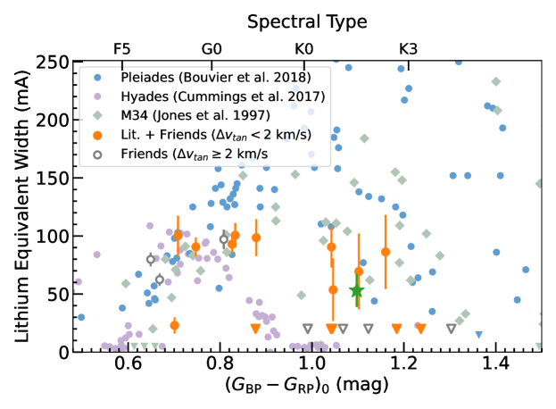
Figure 8: Li equivalent width sequences as a function of Gaia color. Colors have been corrected for reddening. Group-X candidate members from Tang et al. and Fürnkranz et al., and Friends of TOI 2048 with $\Delta v_{tan}<2$ $\rm km~{}s^{-1}$ are shown as large, filled orange circles. Unfilled gray circles are Friends with $\Delta v_{tan}>2$ $\rm km~{}s^{-1}$. TOI 2048 is the green star. Group-X is compared to the Pleiades in blue (blue circles; Bouvier et al. 2018), M34 (green diamonds; Jones et al. 1997), and the Hyades (purple circles; Cummings et al. 2017). All non-detections are plotted as upper limits, denoted by upside-down triangles. The Group-X color-Li sequence lies above the Hyades and below Pleaides; M34 provides the closest match.

4.6 Li-based age

We used the Bayesian Age For Field LowEr mass Stars (BAFFLES; Stanford-Moore et al., 2020) code to derive ages from our individual Li EWs. BAFFLES is a Bayesian framework for deriving age posteriors from Li EWs and $B-V$ colors, and is based on color–Li sequences from NGC 2264 (5.5 Myr), $\beta$ Pic (24 Myr), IC 2602 (44 Myr), $\alpha$ Per (85 Myr), the Pleiades (130 Myr), M35 (200 Myr), M34 (240 Myr), Coma Ber (600 Myr), the Hyades (700 Myr), and M67 (4000 Myr). The ages in parentheses denote those adopted by Stanford-Moore et al. (2020) in their calibration. We adopt the $B-V$ colors from TYCHO (Høg et al., 2000), or where unavailable, APASS (Henden et al., 2015).

We used BAFFLES to measure ages for each star. The median and $1\sigma$ confidence intervals are given in Table 7. We restricted consideration to the 13 stars with Li detections that are either from Tang et al., or from our Friends list and have $\Delta v_{tan}<2$ $\rm km~{}s^{-1}$ (orange circles in Figure 8). From these individual posteriors, we determined an ensemble posterior of the population by multiplying the individual posteriors together. Posteriors are shown in Figure 9. We inferred a final median age of $257\pm 27$ Myr with a 1$\sigma$ error and $257\pm 56$ Myr with a 2$\sigma$ error.

Following Tofflemire et al. (2021), we checked that the final median age was not heavily affected by certain stars. We re-derived our ensemble posterior $10^{4}$ times, sampling with replacement from the 13 stars’ age posteriors. We found that our intrinsic errors dominate over the errors from star selection.

The age derived from Li ($257\pm 27$ Myr) agrees with that assumed based on rotation ($300\pm 50$ Myr) within $1\sigma$. We adopt the rotation-based age for two reasons. First, the coeval groups used by BAFFLES as age-calibrators lack calibrators between $250$ Myr or $600$ Myr. Second, from Figure 8 it is apparent that late G dwarfs provide the most age sensitivity, and there are relatively few such stars in our sample. Therefore, we consider the Li-based age as a means of affirming the age determined through stellar rotation, rather than treating it as an independent age estimate.

Table 7: Li EW Measurements for candidate Group-X members

Name	$G_{\rm BP}-G_{\rm RP}$	$B-V$	RV	$\mathrm{RV}_{\text{err}}$	Li Detection?	EW	$\mathrm{EW}_{\text{err}}$	Age	Ensemble?	SpT
	(mag)	(mag)	$\mathrm{kms}^{-1}$	$\mathrm{kms}^{-1}$		(mÅ)	(mÅ)	(Myr)
Gaia EDR3 1614381144601686528	0.499	0.6	$-$5.05	0.15	0	30.8	47.8	$\cdots$	0	F2.5
Gaia EDR3 1408527485273660416	0.649	0.519	$-$26.28	0.06	1	79.8	6.0	3161	0	F6.6
Gaia EDR3 1595598256183826304	0.668	0.554	14.69	0.05	1	62.4	5.3	3834	0	F7.1
Gaia EDR3 1407864136164159616	0.701	0.533	$-$10.92	0.09	1	23.0	7.0	8222	1	F8.6
Gaia EDR3 1614204913503382784	0.708	0.606	$-$5.05	0.1	1	100.2	17.2	1961	1	F8.9
Gaia EDR3 1403082909850677504	0.747	0.626	$-$6.62	0.08	1	90.6	8.2	1382	1	F9.4
Gaia EDR3 1597089159591345152	0.808	0.659	$-$5.19	0.04	1	97.1	8.3	616	1	G1.5
Gaia EDR3 1593570584944324608	0.826	0.713	$-$5.97	0.06	1	92.9	8.4	331	1	G3.2
Gaia EDR3 1405026605890315776	0.833	0.76	$-$6.89	0.07	1	100.6	10.6	259	1	G3.7
Gaia EDR3 1395517032901515136	0.877	0.825	$-$14.07	0.06	0	20.0	$\cdots$	$\cdots$	0	G7.3
Gaia EDR3 1386467639887852672	0.991	0.876	12.74	0.05	0	20.0	$\cdots$	$\cdots$	0	K0.7
Gaia EDR3 1595101826683842176	1.041	0.789	$-$6.6	0.06	0	20.0	$\cdots$	$\cdots$	0	K1.8
Gaia EDR3 1615219487858308480	1.042	1.094	$-$8.58	0.04	1	90.6	17.8	201	1	K1.8
Gaia EDR3 1403763988584783232	1.044	0.716	$-$6.64	0.06	0	20.0	$\cdots$	$\cdots$	0	K1.8
Gaia EDR3 1599791690453687168	1.046	1.047	$-$5.62	0.05	1	53.7	27.0	362	1	K1.8
Gaia EDR3 1424042006658262784	1.067	0.874	$-$3.23	0.06	0	20.0	$\cdots$	$\cdots$	0	K1.9
Gaia EDR3 1404488390652463872	1.097	1.02	$-$7.37	0.04	1	53.1	14.1	285	1	K2.1
Gaia EDR3 1614271571396149120	1.102	1.364	$-$11.07	0.11	1	69.4	32.6	157	1	K2.1
Gaia EDR3 1401952440098841984	1.123	1.062	$-$2.28	0.07	0	20.0	$\cdots$	$\cdots$	0	K2.3
Gaia EDR3 1596427940786153728	1.16	0.818	$-$6.31	0.07	1	86.2	31.9	492	1	K2.7
Gaia EDR3 1384397564433951744	1.185	1.427	$-$5.08	0.07	0	13.7	18.2	$\cdots$	0	K2.9
Gaia EDR3 1617388377623238272	1.237	1.81	$-$5.02	0.15	0	20.0	$\cdots$	$\cdots$	0	K3.4
Gaia EDR3 1597757387783227008	1.303	1.408	$-$7.77	0.08	0	20.0	$\cdots$	$\cdots$	0	K3.9

Note. — Non-detections are included with EW $=20.0$ mÅ. In the ensemble posterior calculation, we only include likely members of Group-X using the velocity offset cut discussed in §4.3. Spectral types are approximated from Gaia $G_{\rm BP}-G_{\rm RP}$ colors and included for informational purposes (Pecaut & Mamajek 2013, as updated at https://www.pas.rochester.edu/~emamajek/EEM_dwarf_UBVIJHK_colors_Teff.txt). This table is available in its entirety in a machine-readable form in the online journal. A portion is shown here for guidance regarding its form and content.

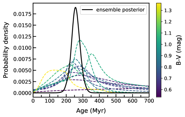
Figure 9: Li–age posteriors from BAFFLES. Individual age posteriors as dashed lines colored by stars’ $B-V$ magnitudes. The ensemble posterior shown in solid black line, and has been divided by two for visual purposes. The median age of Group-X is $257\pm 27$ Myr.

4.7 Opportunity for an asteroseismic age

Asteroseismology of high-frequency $\delta$ Scuti stars has recently emerged as a powerful tool to independently determine ages of young moving groups and associations (Bedding et al., 2020; Murphy et al., 2021). We analyzed the hottest stars in Group-X and detected clear $\delta$ Scuti pulsations in TIC 137834492 (HD 133909, $Bp-Rp=0.235$, $T=7.2$, Figure 10). The pulsations have an period of around 0.6 hours and show an apparent spacing of a few c/d, consistent with other young $\delta$ Scuti stars for which mode identification has been possible. A detailed asteroseismic analysis is beyond the scope of this paper, but the detection of a high-frequency $\delta$ Scuti star is consistent with the young age for Group-X.

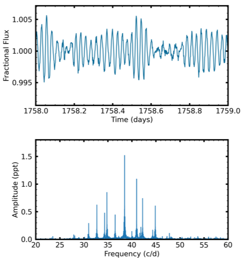
Figure 10: Top panel: 1 day segment of the 2-minute light curve of TIC137834492 showing multiperiodic, high-frequency pulsations characteristic of young $\delta$ Scuti stars. Bottom panel: amplitude spectrum of the full 2-minute light curve (Sectors 16, 22 and 23) centered on the pulsations.

TIC 459221499 (HD 116798) shows $\gamma$ Doradus pulsations (Balona et al. 1994). Additional data may yield a regular gravity mode pattern and thus open up the possibility of an asteroseismic age (T. Bedding, priv. comm.).

5 Transit Analysis

5.1 TOI 2048 Transit modeling

We used MCMC to derive the physical parameters of TOI 2048 from the TESS SAP light curve. The observed light curve was fit as a sum of intrinsic stellar variability and variation owing to the planetary transit. We modeled the stellar variability using exoplanet with the same Gaussian Process model described in §3.3.1: a quasiperiodic kernel associated with stellar rotation. We placed Gaussian priors on each parameter using the mean and standard deviation of the posteriors from our rotation-only fit.

To model the transit, we used exoplanet to set up a Keplerian orbit with the stellar density ($\rho_{\star}$), stellar radius ($R_{\star}$), stellar limb darkening ($u_{1}$, $u_{2}$), log planetary radius in units of $R_{\star}$ ($\log{r}$), impact parameter ($b$), orbital period ($P_{p}$), and reference transit time ($T_{0}$). Our stellar radius and density are constrained by Gaussian priors with means and standard deviations taken from Table 2. Limb darkening was sampled uninformatively following Kipping (2013a) and the impact parameter was constrained to be between 0 and 1. We used uninformative priors on the remaining planetary parameters. We performed a circular fit, and one where the eccentricity $e$ and argument of periastron $\omega$ were allowed to vary; for the eccentric fit, we use the supplied prior from Kipping (2013b) for the eccentricity.

We input initial guesses for the planetary radius, orbital period, and reference transit time from ExoFOP. We then used pymc3’s find_MAP to fit each parameter individually, and then optimized across all variables. We masked data points lying $>5\sigma$ from the best-fit model, and re-fit the model. This maximum a posteriori fit provided the starting location to our MCMC sampling. Finally, we sampled the parameter space using pymc3’s NUTS sampler (using the masked data). We took 4000 tuning steps and 4000 draws, using six chains. We used an initial acceptance rate of 0.7 that was increased to 0.99 during tuning. The Gelman-Rubin statistic $\hat{R}$ values was $1.0$ for all parameters and there were no divergences after tuning (which would indicate regions of parameter space that may not have been effectively explored), indicating convergence.

Each individual transit and model is shown in Figure 11. The phased transit light curve with the stellar variability model removed in shown in Figure 12. Our transit parameters are given in Table 8; the planet radius is $2.1\pm 0.2$ $R_{\earth}$ and the period is $13.8$ d. The fits with $e$ fixed to $0$ and variable $e$ are consistent, with moderate eccentricities allowed, but not required, by the data ($e=0.13^{+0.18}_{-0.09}$, with the $2\sigma$ confidence interval extending from $0.007$ to $0.4$).

We also ran our transit fit using our custom reduction of the two minute cadence data (shown in Fig. 1). This reduction used additional systematics corrections not included in the SAP lightcurve we used for the above analysis. The differences were insignificant.

Table 8: Fitted and derived planetary parameters

Parameter	Value
	$e$, $\omega$ fixed	$e$, $\omega$ free
Fitted parameters
$T_{0}$ (TJD)	$1739.1171^{+0.012}_{-0.0085}$	$1739.1174^{+0.012}_{-0.0087}$
$P_{p}$ (days)	$13.79021^{+0.00063}_{-0.00085}$	$13.79019^{+0.00065}_{-0.00084}$
$\log{R_{P}/R_{\odot}}$	$-3.741^{+0.064}_{-0.066}$	$-3.735\pm 0.066$
$b$	$0.29^{+0.16}_{-0.19}$	$0.33^{+0.22}_{-0.21}$
$\rho_{\star}$	$2.42^{+0.33}_{-0.34}$	$2.38^{+0.35}_{-0.36}$
$u_{\star,0}$	$0.31^{+0.57}_{-0.51}$	$0.31^{+0.59}_{-0.53}$
$u_{\star,1}$	$0.31^{+0.59}_{-0.54}$	$0.31^{+0.58}_{-0.52}$
$\sqrt{e}\cos{\omega}$	$\cdots$	$-0.04^{+0.29}_{-0.3}$
$\sqrt{e}\sin{\omega}$	$\cdots$	$-0.04^{+0.3}_{-0.28}$
Derived parameters
$a/R_{\star}$	$32.5^{+1.4}_{-1.6}$	$32.9^{+1.9}_{-1.8}$
$R_{P}/R_{\odot}$	$0.0237^{+0.0016}_{-0.0015}$	$0.0239^{+0.0016}_{-0.0015}$
$R_{P}$ ($R_{\earth})$	$2.59^{+0.17}_{-0.16}$	$2.61^{+0.17}_{-0.16}$
$i$ ($\degree$)	$89.49^{+0.33}_{-0.32}$	$89.41^{+0.39}_{-0.42}$
$e$	$\cdots$	$0.13^{+0.18}_{-0.09}$
$\Omega$ ($\degree$)	$\cdots$	$-0.4^{+2.4}_{-2.1}$

Note. — We adopted the fit with variable $e$, $\omega$.

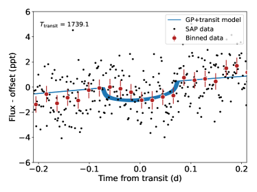
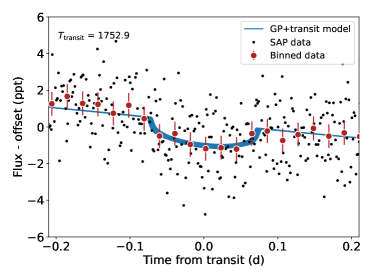
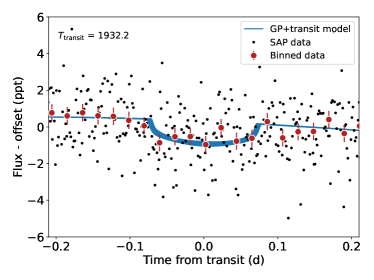
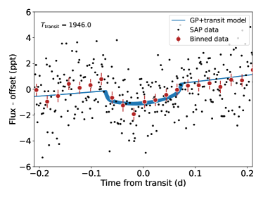
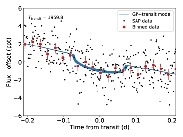
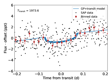
Figure 11: Individual transits for TOI 2048 b. Time is in days from transit center; the time of transit is given in the upper right in TJBD. Flux is in ppt with vertical offset applied. Small gray points show the TESS-SAP data after outliers have been removed. The larger red points show the binned data with error bars; the error bars are similar in size to the data points. Bins are 30 minutes; the points are the weighted average and the error bars are the standard error on the means. The blue shaded region shows the $1\sigma$ range of the model (stellar variability GP plus transit).

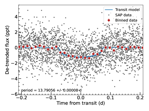
Figure 12: Phase-folded transit light curve for TOI 2048 b, detrending using the stellar rotation model. Time is in units of days, and the flux is in ppt. Small gray points show the TESS-SAP data after outliers have been removed and the stellar variability model has been removed. The larger red points show the binned data with error bars; the error bars are similar in size to the data points. Bins are 20 minutes; the points are the weighted average and the error bars are the standard error on the means. The blue shaded region shows the $1\sigma$ range of the transit model.

5.2 Statistical validation

We consider false positive scenarios to statistically validate TOI 2048 b using two tools. We use Multi Observational Limits on Unseen Stellar Companions code (MOLUSC; Wood et al., 2021) and the Tool for Rating Interesting Candidate Exoplanets and Reliability Analysis of Transits Originating from Proximate Stars (TRICERATOPS; Giacalone et al., 2021).

5.2.1 MOLUSC

With MOLUSC , we explore the range of possible bound companions to the planet host that could produce the observed transit. To briefly summarize, MOLUSC simulates realistic stellar companions following a physically motivated distribution of physical parameters (period, mass ratio, etc). For each companion, it compares the expected signal to the observed high-resolution imaging, radial velocities, and limits from Gaia imaging and astrometry. Companions are eliminated if they should have been recovered in the data, and survive if not.

For TOI 2048, we generated one million companions, using all available constraints from Section 2 and the stellar parameters from Section 3.1. Of the generated companions, 8.5% survive the comparison. Most are stars that are on wide orbits and happen to be behind the target at the moment of observations, brown dwarfs that are below our imaging detection thresholds, or close-in objects on face-on orbits that elude the velocity constraints.

None of the surviving companions transit the host at the detected period, ruling out the possibility of an eclipsing binary. A hierarchical binary cannot be ruled out, but it is highly disfavored. Assuming the deepest possible eclipse is 50%, none of the companions below $\simeq 0.3\text{M}_{\odot}$ ($q\simeq 0.37$) can reproduce the transit. Only about 10% of the surviving companions pass this criterion (0.85% of the original generated sample).

5.2.2 TRICERATOPS

With TRICERATOPS, we statistically validate TOI 2048 b. TRICERATOPS leverages Gaia DR2 and the TESS Input Catalog (TIC) to consider false positive probabilities for nearby stars, many of which are blended with the target star due to TESS’s large pixel size. TRICERATOPS considers contamination of the target star aperture from stars within 10 pixels of the target that are listed in the TIC. The false positive scenarios that are modeled as possible origins of the putative transit signal include both bound stellar companions and background stars, and both eclipsing binaries and transiting planets other than the planet under consideration. We used the phase-folded two minute cadence data detrended with the Gaussian process stellar variability model, which we bin for computational ease.

Background eclipsing binaries represented the most likely false positive for our data, so the limits on background sources from AO imaging were an important constraint. Our primary constraint was the NIRC2 contrast curve. The $\Delta K=8.3$ quoted at 2″ in Table 1 applies out to $5$″, since from 2–5″ background noise is the limiting magnitude. Beyond $5$″, Gaia provided strong constraints. As there are no stars within $44$″ of TOI 2048 in Gaia, we adopted $\Delta K=15$ as the contrast limit from $5-25$″. At separations below $0.15$″, we approximated the RUWE limits as $\Delta K=0$ at $0.03$″, and $\Delta K=3$ at $0.08$″.

We used TRICERATOPS to simulate the possible scenarios that could produce the observed transit, applying the composite $K$ band contrast curve as a constraint. We created $10^{6}$ realizations and calculated the false positive probability (FPP) and nearby false positive probability (NFPP). The NFPP describes the probability that a false positive scenario arises due to a known nearby star. We then repeated the experiment 10 times, and took the mean and standard deviation of the resulting rates. NFPP is $0$. The FPP from 10 trials is $0.0011\pm 0.0001$.

Giacalone et al. (2021) established criteria of FPP$<0.015$ and NFPP$<10^{-3}$; thus, we consider TOI 2048 b statistically validated.

5.3 Prospects for further follow-up

Its young age, moderate orbital period, and small size make TOI-2048 an interesting target for atmospheric studies, but these characteristics also pose a challenge. Assuming zero albedo and full day-night heat redistribution, TOI-2048 b has an equilibrium temperature $T_{\rm eq}=640\pm 20$ K. We find that the target is unfavorable for JWST observations with transmission and emission spectroscopy metrics (TSM, ESM; Kempton et al. 2018) of 25 and 1, respectively. Atmospheric escape could help probe mass-loss mechanisms for small planets (e.g, Owen & Wu, 2017; Ginzburg et al., 2018), though young exoplanets pose a variety of challenges (e.g. Palle et al., 2020; Benatti et al., 2021; Rockcliffe et al., 2021). However, the host star is relatively bright ($V=11.5$, $K=9.4$) and observations with ground-based large or future extremely large telescopes are feasible.

We searched the 30-minute cadence FFI data for additional transiting planets in the system (Vanderburg et al., 2016) and found no candidates.

The 20 April 2022 data obtained with LCO 2.1.2 and MuSCAT2 2.2 while this work was under review suggest the transit occurs 20-25 minutes later than the ephemeris presented in this paper. This target also continues to be observed in TESS Cycle 4.

6 Summary and discussion

We have presented a new analysis of Group-X, found serendipitously in two studies of Coma Ber by Tang et al. (2019) and Fürnkranz et al. (2019), and the exoplanetary system that is a member of this association.

We identified 139 new candidate members of Group-X using the FindFriends algorithm (§4.1) of which we suggest that the 46 with $\Delta v_{tan}<2$ $\rm km~{}s^{-1}$ are likely members. We measured rotation periods for Group-X candidate members from TESS and ZTF photometry (§4.3), from which we determined that the gyrochronological age of Group-X is a close match to that of NGC 3532 (Fritzewski et al., 2019, 2021). We therefore adopted an age of $300\pm 50$ Myr for Group-X. We also obtained new optical spectra of candidate Group-X members and measured lithium for 23 stars; the Li sequence for Group-X confirmed an age of a few hundred Myr (§4.5). Group-X joins NGC 3532 as an accessible cluster of intermediate age between the well-studied Pleaides, Prasepe and Hyades clusters. With further study into its membership and age, it could prove to be an important benchmark for constraining spin-down (e.g. the age at which the sequence of rapid rotators disappears) and Li depletion.

We identified several stars of interest. There are two eclipsing binaries (TIC 441702640 and TIC 165407465), and a white dwarf (TIC 1200926232) that could plausibly have an age consistent with the cluster. $\delta$ Scuti (TIC 137834492, HD 133909) and $\gamma$ Doradus (TIC 459221499, HD 116798) pulsators offer the opportunity for an asteroseismic age determination (§4.7).

We serendipitously found a new, small candidate association nearby to Group-X, which we call MELANGE-2 (Appendix A). We measured rotation periods for the candidate members of MELANGE-2, which suggest an age similar to Praesepe ($\sim 700$ Myr).

Turning to the exoplanet, we found that TOI 2048 is a late G dwarf with 80% the mass and radius of the Sun and an effective temperature of $5200$ K. Our panoply of high-contrast imaging and analysis of Gaia data indicate that TOI 2048 has no stellar companions or nearby neighbors. Using two different statistical tools, MOLUSC (Wood et al., 2021) and TRICERATOPS (Giacalone et al., 2021), we statistically validate TOI 2048 b. Modeling of the TESS transit data reveals a planet with a period of $13.8$ days and a radius of $2.6\pm 0.2$ Earth radii. The planet falls within the mini-Neptune part of parameter space that is well-populated by both field stars and other young planets with ages $\sim$250–700 Myr (Figure 13, Table 9).

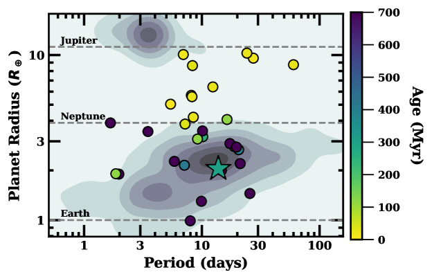
Figure 13: Exoplanets from the NASA Exoplanet Archive NASA Exoplanet Science Institute (2020) a function of planet radius ($R_{\oplus}$) and orbital period (days). Contours show all planets from Kepler and K2. Young ($<$1 gyr), transiting planets part of open star clusters or associations are plotted in circles colored by their age; data for these planets are listed in Table 9. TOI 2048 b is outlined as a star and lands in the main distribution of its older counterparts.

Planet Name	Cluster	Age	Planet radius	Orbital period	Provenance
		(Myr)	$R_{\earth}$	d
AU Mic b	Beta Pictoris	22	4.20	8.463	Plavchan et al. (2020)
AU Mic c	Beta Pictoris	22	2.79	18.859	Gilbert et al. (2022)
DS Tuc A b	Tucana–Horologium	40	5.70	8.138	Newton et al. (2019)
EPIC 211822797 b	Praesepe	700	2.20	21.170	Mann et al. (2017)
HD 110082 b	MELANGE-1	250	3.20	10.183	Tofflemire et al. (2021)
HD 63433 b	Ursa Major	414	2.15	7.108	Mann et al. (2020)
HD 63433 c	Ursa Major	414	2.67	20.545	Mann et al. (2020)
HIP 67522 b	Sco-Cen OB	17	10.07	6.960	Rizzuto et al. (2020)
K2-100 b	Praesepe	700	3.88	1.674	Barragán et al. (2019)
K2-101 b	Praesepe	700	2.00	14.677	Mann et al. (2017)
K2-102 b	Praesepe	700	1.30	9.916	Mann et al. (2017)
K2-104 b	Praesepe	700	1.90	1.974	Mann et al. (2017)
K2-136 b	Hyades	700	0.99	7.975	Mann et al. (2018)
K2-136 c	Hyades	700	2.91	17.307	Mann et al. (2018)
K2-136 d	Hyades	700	1.45	25.575	Mann et al. (2018)
K2-25 b	Hyades	700	3.44	3.485	Stefansson et al. (2020)
K2-264 b	Praesepe	700	2.27	5.840	Rizzuto et al. (2018)
K2-264 c	Praesepe	700	2.77	19.663	Rizzuto et al. (2018)
K2-33 b	Upper Sco	9	5.04	5.425	Mann et al. (2016b)
K2-95 b	Praesepe	700	3.47	10.134	Obermeier et al. (2016)
Kepler-1627 b	Delta Lyra	38	3.82	7.203	Bouma et al. (2022)
TOI-1227 b	Epsilon Cha	11	9.57	27.364	Mann et al. (2022)
TOI-451 b	Pisces–Eridanus	120	1.91	1.859	Newton et al. (2021)
TOI-451 c	Pisces–Eridanus	120	3.10	9.193	Newton et al. (2021)
TOI-451 d	Pisces–Eridanus	120	4.07	16.365	Newton et al. (2021)
TOI-837 b	IC 2602	35	8.63	8.325	Bouma et al. (2020)
V1298 Tau b	Taurus	23	10.27	24.140	David et al. (2019b)
V1298 Tau c	Taurus	23	5.59	8.250	David et al. (2019a)
V1298 Tau d	Taurus	23	6.41	12.403	David et al. (2019a)
V1298 Tau e	Taurus	23	8.74	60.000	David et al. (2019a)

Table 9: Provenance of data for transiting planets in associations $<1$ Gyr in age, plotted in Figure 13. Data taken from NASA Exoplanet Science Institute (2020).

Appendix A Serendipitous discovery of another candidate young group

In our rotation analysis of Group-X candidate members, we found a relatively high rate of rotation period detections at large $\Delta v_{tan}$. However, stars with tangential velocities offset $4-5$ $\rm km~{}s^{-1}$ from TOI 2048 are unlikely to be part of Group-X. There also appeared to be a small clustering of stars with detected rotation periods in both position and proper motion space, offset from Group-X.

Motivated by this, we ran FindFriends centered on TIC 224606446, for which we detect a rotation period but which has $\Delta v_{tan}=5$. We selected this star because it appears in the small outlying clusters in both position and proper motion, and had a radial velocity measurement available (required for this analysis). We searched in a 20pc volume with a limit of $\Delta v_{tan}<4$ $\rm km~{}s^{-1}$; the smaller search area was intended to limit the number of Group-X stars picked up in the search. The results are shown in Figure 14. There is a clear clustering of stars with similar tangential velocities in position space, and the radial velocities are in good agreement for the six stars (besides TIC 224606446 itself) with such measurements. This suggests that the small group is a physically associated. Table 10 lists the 81 Friends of 224606446.

This group does not appear in the Theia catalog (Kounkel & Covey, 2019), and to our knowledge is not previously known. We call this group MELANGE-2 (Membership and Evolution by Leveraging Adjacent Neighbors in a Genuine Ensemble), following the nomenclature established for these small “Friends” associations in Tofflemire et al. (2021). MELANGE-2 is the second cluster serendipitously discovered in the vicinity of Coma Ber.

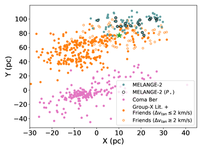
Figure 14: Galactic positions for MELANGE-2 (gray-blue), Group-X (orange), and Coma Ber (pink). TOI 2048, a Group-X candidate member, is marked by the green star. MELANGE-2 candidate members with rotation periods detected in TESS are outlined in black. Data for Coma Ber comes from Tang et al. (2019). For Group-X, candidate members from Tang et al. and Fürnkranz et al., and Friends of TOI 2048 with $\Delta v_{tan}<2$ $\rm km~{}s^{-1}$ are shown as filled orange circles. Unfilled orange circles are Friends with $\Delta v_{tan}>2$ $\rm km~{}s^{-1}$. There is some overlap between Group-X (especially Friends with $\Delta v_{tan}>2$ $\rm km~{}s^{-1}$) and MELANGE-2.

We then measured rotation periods for the Friends of TIC 224606446 as was done in §4.3, searching both SPOC SAP light curves and our own FFI light curves. MELANGE-2 candidate members and stellar rotation periods are given in Table 11 and shown in Figure 15. Assuming this association is real, Figure 15 suggests it is similar in age to Praesepe.

An open question is how certain we can be that small clusters such as MELANGE-2 are true physical associations. Within $\pm 2$hrs of TOI-2048 and $\delta>0\degree$, our team has previously used FindFriends to look for associations surrounding six other stars of interest. Only one of the six has a small, convincing association, so groupings similar to MELANGE-2 are not likely common.

The rotation periods also provide evidence that the association is bonafide. We measure 18 secure periods for a detection fraction of $22\pm 5$%. Including the additional nine candidate periods would give a detection fraction of $33\pm 6$%. This is significantly lower than the detection fraction for Group-X, but still higher than what we would expect from the field: in Kepler, $14-16$% of stars have $P_{rot}<18$ d (McQuillan et al., 2014; Santos et al., 2021). Friends of TIC 224606446 also do not have periods that fall randomly, but instead align with Praesepe (Fig. 15). Due to the temporary pause in spin down (Agüeros et al., 2018; Curtis et al., 2020), it is possible that this agreement is a coincidence. We tested this by drawing 13 random stars (our sample of secure and candidate detections excluding the five mid M dwarfs that are not well-represented in Kepler) from the Kepler sample of McQuillan et al. (2014). We repeated this 100 times, visually comparing the results to Praesepe on a log-period versus temperature plot. Three of the samples had some visual similarity to Praesepe, but were not as good a match as Friends of TIC 224606446. Further work is needed to accurately quantify this comparison due to the partial overlap with Group-X, and due to TESS’s diminished sensitivity to rotation periods $>10$ d compared to Kepler.

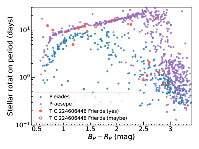
Figure 15: Rotation periods for Friends of TIC 224606446 (larger red-orange circles) showing both secure period detections (filled circles) and candidate periods (open circles). There is some overlap with Friends of TOI 2048. Also shown are rotation periods of benchmark clusters Pleiades (small blue circles) and Praesepe (small purple circles). Friends of TIC 224606446 generally lie along the sequence defined by Praesepe.

Table 10: Friends of MELANGE-2

Gaia source ID	R.A.	Dec	$G$	$G_{\rm BP}-G_{\rm RP}$	Gaia RUWE	$\pi$	TIC ID	$T_{\mathrm{mag}}$
	deg	deg	mag	mag		mas		mag
1420124068771090048	255.730252	54.3406952	12.212	1.362	1.039	8.391	224606446	11.531
1419817889142291968	256.3677107	53.5801456	16.27	3.027	1.018	8.432	274696733	14.923
1419195428122063232	258.7673411	54.2611273	14.547	2.240	0.948	8.425	198393082	13.459
1413990168277612928	253.8912148	52.8723173	11.934	1.277	1.149	8.515	274509064	11.289
1420409426397997440	259.3583692	55.219843	16.833	3.143	4.087	8.463	198413773	15.320

Note. — This table is included in its entirety online as a machine readable table.

Table 11: Rotation periods for MELANGE-2 Friends

TIC ID	$T_{\mathrm{mag}}$	TESS Contam. ratio	Gaia RUWE	$G_{\rm BP}-G_{\rm RP}$	TESS note	$P_{\star}$
	mag			mag		d
188774365	5.70303	0.0	0.964	0.210	y	0.12
188692788	8.60509	0.0	1.43	0.701	y	12
367814788	9.63893	0.07	11.548	0.799	y	10
274575202	9.11923	0.02	1.057	0.921	eb	5.7
274274478	9.6454	$\cdots$	8.273	0.994	y	16

Note. — This table is included in its entirety online as a machine readable table.

References

- Agüeros et al. (2018) Agüeros, M. A., Bowsher, E. C., Bochanski, J. J., et al. 2018, ApJ, 862, 33, doi: 10.3847/1538-4357/aac6ed
- Albareti et al. (2017) Albareti, F. D., Allende Prieto, C., Almeida, A., et al. 2017, ApJS, 233, 25, doi: 10.3847/1538-4365/aa8992
- Balona et al. (1994) Balona, L. A., Krisciunas, K., & Cousins, A. W. J. 1994, MNRAS, 270, 905, doi: 10.1093/mnras/270.4.905
- Baraffe et al. (2015) Baraffe, I., Homeier, D., Allard, F., & Chabrier, G. 2015, Astronomy & Astrophysics, 577, A42, doi: 10.1051/0004-6361/201425481
- Baraffe et al. (2015) Baraffe, I., Homeier, D., Allard, F., & Chabrier, G. 2015, A&A, 577, A42, doi: 10.1051/0004-6361/201425481
- Barnes (2003) Barnes, S. A. 2003, The Astrophysical Journal, 586, 464, doi: 10.1086/367639
- Barragán et al. (2019) Barragán, O., Aigrain, S., Kubyshkina, D., et al. 2019, MNRAS, 490, 698, doi: 10.1093/mnras/stz2569
- Bedding et al. (2020) Bedding, T. R., Murphy, S. J., Hey, D. R., et al. 2020, Nature, 581, 147, doi: 10.1038/s41586-020-2226-8
- Bellm et al. (2019a) Bellm, E. C., Kulkarni, S. R., Graham, M. J., et al. 2019a, PASP, 131, 018002, doi: 10.1088/1538-3873/aaecbe
- Bellm et al. (2019b) —. 2019b, PASP, 131, 018002, doi: 10.1088/1538-3873/aaecbe
- Belokurov et al. (2020) Belokurov, V., Penoyre, Z., Oh, S., et al. 2020, MNRAS, 496, 1922, doi: 10.1093/mnras/staa1522
- Benatti et al. (2021) Benatti, S., Damasso, M., Borsa, F., et al. 2021, A&A, 650, A66, doi: 10.1051/0004-6361/202140416
- Blackwell & Shallis (1977) Blackwell, D. E., & Shallis, M. J. 1977, MNRAS, 180, 177, doi: 10.1093/mnras/180.2.177
- Bodenheimer (1965) Bodenheimer, P. 1965, The Astrophysical Journal, 142, 451, doi: 10.1086/148310
- Bohlin et al. (2020) Bohlin, R. C., Hubeny, I., & Rauch, T. 2020, The Astronomical Journal, 160, 21, doi: 10.3847/1538-3881/ab94b4
- Bouma et al. (2020) Bouma, L. G., Hartman, J. D., Brahm, R., et al. 2020, AJ, 160, 239, doi: 10.3847/1538-3881/abb9ab
- Bouma et al. (2022) Bouma, L. G., Curtis, J. L., Masuda, K., et al. 2022, AJ, 163, 121, doi: 10.3847/1538-3881/ac4966
- Bouvier et al. (2018) Bouvier, J., Barrado, D., Moraux, E., et al. 2018, A&A, 613, A63, doi: 10.1051/0004-6361/201731881
- Brandeker & Cataldi (2019) Brandeker, A., & Cataldi, G. 2019, Astronomy and Astrophysics, 621, A86, doi: 10.1051/0004-6361/201834321
- Brasseur et al. (2019) Brasseur, C. E., Phillip, C., Fleming, S. W., Mullally, S. E., & White, R. L. 2019, Astrocut: Tools for creating cutouts of TESS images. http://ascl.net/1905.007
- Bressan et al. (2012) Bressan, A., Marigo, P., Girardi, L., et al. 2012, Monthly Notices of the Royal Astronomical Society, 427, 127, doi: 10.1111/j.1365-2966.2012.21948.x
- Brown et al. (2013) Brown, T. M., Baliber, N., Bianco, F. B., et al. 2013, Publications of the Astronomical Society of the Pacific, 125, 1031, doi: 10.1086/673168
- Bryson et al. (2020) Bryson, S., Coughlin, J., Batalha, N. M., et al. 2020, The Astronomical Journal, 159, 279, doi: 10.3847/1538-3881/ab8a30
- Buchhave et al. (2010) Buchhave, L. A., Bakos, G. Á., Hartman, J. D., et al. 2010, ApJ, 720, 1118, doi: 10.1088/0004-637X/720/2/1118
- Chaplin & Miglio (2013) Chaplin, W. J., & Miglio, A. 2013, ARA&A, 51, 353, doi: 10.1146/annurev-astro-082812-140938
- Chen et al. (2015) Chen, Y., Bressan, A., Girardi, L., et al. 2015, Monthly Notices of the Royal Astronomical Society, 452, 1068, doi: 10.1093/mnras/stv1281
- Chen et al. (2019) Chen, Y., Girardi, L., Fu, X., et al. 2019, Astronomy and Astrophysics, 632, A105, doi: 10.1051/0004-6361/201936612
- Clem et al. (2011) Clem, J. L., Landolt, A. U., Hoard, D. W., & Wachter, S. 2011, The Astronomical Journal, 141, 115, doi: 10.1088/0004-6256/141/4/115
- Collaboration et al. (2021) Collaboration, G., Brown, A. G. A., Vallenari, A., et al. 2021, Astronomy and Astrophysics, 649, A1, doi: 10.1051/0004-6361/202039657
- Collins et al. (2017) Collins, K. A., Kielkopf, J. F., Stassun, K. G., & Hessman, F. V. 2017, The Astronomical Journal, 153, 77, doi: 10.3847/1538-3881/153/2/77
- Cummings et al. (2017) Cummings, J. D., Deliyannis, C. P., Maderak, R. M., & Steinhauer, A. 2017, AJ, 153, 128, doi: 10.3847/1538-3881/aa5b86
- Curtis et al. (2020) Curtis, J. L., Agüeros, M. A., Matt, S. P., et al. 2020, The Astrophysical Journal, 904, 140, doi: 10.3847/1538-4357/abbf58
- David et al. (2019a) David, T. J., Petigura, E. A., Luger, R., et al. 2019a, ApJ, 885, L12, doi: 10.3847/2041-8213/ab4c99
- David et al. (2016) David, T. J., Conroy, K. E., Hillenbrand, L. A., et al. 2016, AJ, 151, 112, doi: 10.3847/0004-6256/151/5/112
- David et al. (2019b) David, T. J., Cody, A. M., Hedges, C. L., et al. 2019b, AJ, 158, 79, doi: 10.3847/1538-3881/ab290f
- Dekany et al. (2013) Dekany, R., Roberts, J., Burruss, R., et al. 2013, ApJ, 776, 130, doi: 10.1088/0004-637X/776/2/130
- Dotter et al. (2008) Dotter, A., Chaboyer, B., Jevremović, D., et al. 2008, ApJS, 178, 89, doi: 10.1086/589654
- Douglas et al. (2019) Douglas, S. T., Curtis, J. L., Agüeros, M. A., et al. 2019, The Astrophysical Journal, 879, 100, doi: 10.3847/1538-4357/ab2468
- Doyle et al. (2014) Doyle, A. P., Davies, G. R., Smalley, B., Chaplin, W. J., & Elsworth, Y. 2014, MNRAS, 444, 3592, doi: 10.1093/mnras/stu1692
- Ester et al. (1996) Ester, M., Kriegel, H.-P., Sander, J., & Xu, X. 1996, in Proceedings of the Second International Conference on Knowledge Discovery and Data Mining
- ExoFOP (2019) ExoFOP. 2019, Exoplanet Follow-up Observing Program - TESS, IPAC, doi: 10.26134/EXOFOP3
- Faherty et al. (2018) Faherty, J. K., Bochanski, J. J., Gagné, J., et al. 2018, The Astrophysical Journal, 863, 91, doi: 10.3847/1538-4357/aac76e
- Fausnaugh et al. (2020) Fausnaugh, M. M., Burke, C. J., Ricker, G. R., & Vanderspek, R. 2020, Research Notes of the American Astronomical Society, 4, 251, doi: 10.3847/2515-5172/abd63a
- Fitton et al. (2022) Fitton, S., Tofflemire, B. M., & Kraus, A. L. 2022, Research Notes of the American Astronomical Society, 6, 18, doi: 10.3847/2515-5172/ac4bb7
- Foreman-Mackey (2016) Foreman-Mackey, D. 2016, The Journal of Open Source Software, 1
- Foreman-Mackey (2018) Foreman-Mackey, D. 2018, Research Notes of the American Astronomical Society, 2, 31, doi: 10.3847/2515-5172/aaaf6c
- Foreman-Mackey et al. (2017) Foreman-Mackey, D., Agol, E., Ambikasaran, S., & Angus, R. 2017, The Astronomical Journal, 154, 220, doi: 10.3847/1538-3881/aa9332
- Foreman-Mackey et al. (2021) Foreman-Mackey, D., Luger, R., Agol, E., et al. 2021, Journal of Open Source Software, 6, 3285, doi: 10.21105/joss.03285
- Fritzewski et al. (2019) Fritzewski, D. J., Barnes, S. A., James, D. J., et al. 2019, Astronomy & Astrophysics, 622, A110, doi: 10.1051/0004-6361/201833587
- Fritzewski et al. (2021) Fritzewski, D. J., Barnes, S. A., James, D. J., & Strassmeier, K. G. 2021, Astronomy & Astrophysics, 652, A60, doi: 10.1051/0004-6361/202140894
- Fűrész et al. (2008) Fűrész, G., Szentgyorgyi, A. H., & Meibom, S. 2008, Precision of Radial Velocity Surveys Using Multiobject Spectrographs — Experiences with Hectochelle, 287–290, doi: 10.1007/978-3-540-75485-5_68
- Fürnkranz et al. (2019) Fürnkranz, V., Meingast, S., & Alves, J. 2019, A&A, 624, L11, doi: 10.1051/0004-6361/201935293
- Gaia Collaboration et al. (2016) Gaia Collaboration, Prusti, T., de Bruijne, J. H. J., et al. 2016, Astronomy and Astrophysics, 595, A1, doi: 10.1051/0004-6361/201629272
- Gaia Collaboration et al. (2018) Gaia Collaboration, Brown, A. G. A., Vallenari, A., et al. 2018, Astronomy and Astrophysics, 616, A1, doi: 10.1051/0004-6361/201833051
- Gaia Collaboration et al. (2021) Gaia Collaboration, Brown, A. G. A., Vallenari, A., et al. 2021, A&A, 649, A1
- Gavel et al. (2014) Gavel, D., Kupke, R., Dillon, D., et al. 2014, in Society of Photo-Optical Instrumentation Engineers (SPIE) Conference Series, Vol. 9148, Adaptive Optics Systems IV, ed. E. Marchetti, L. M. Close, & J.-P. Vran, 914805, doi: 10.1117/12.2055256
- Giacalone et al. (2021) Giacalone, S., Dressing, C. D., Jensen, E. L. N., et al. 2021, The Astronomical Journal, 161, 24, doi: 10.3847/1538-3881/abc6af
- Gilbert et al. (2022) Gilbert, E. A., Barclay, T., Quintana, E. V., et al. 2022, AJ, 163, 147, doi: 10.3847/1538-3881/ac23ca
- Ginsburg et al. (2019) Ginsburg, A., Sipőcz, B. M., Brasseur, C. E., et al. 2019, The Astronomical Journal, 157, 98, doi: 10.3847/1538-3881/aafc33
- Ginzburg et al. (2018) Ginzburg, S., Schlichting, H. E., & Sari, R. 2018, MNRAS, 476, 759, doi: 10.1093/mnras/sty290
- Goodman & Weare (2010) Goodman, J., & Weare, J. 2010, COMM. APP. MATH. AND COMP. SCI, 5
- Gray (2008) Gray, D. F. 2008, The Observation and Analysis of Stellar Photospheres
- Green et al. (2019) Green, G. M., Schlafly, E., Zucker, C., Speagle, J. S., & Finkbeiner, D. 2019, The Astrophysical Journal, 887, 93, doi: 10.3847/1538-4357/ab5362
- Guerrero et al. (2021) Guerrero, N. M., Seager, S., Huang, C. X., et al. 2021, The Astrophysical Journal Supplement Series, 254, 39, doi: 10.3847/1538-4365/abefe1
- Hayward et al. (2001) Hayward, T. L., Brandl, B., Pirger, B., et al. 2001, PASP, 113, 105, doi: 10.1086/317969
- Henden et al. (2015) Henden, A. A., Levine, S., Terrell, D., & Welch, D. L. 2015, 225, 336.16
- Henden et al. (2012) Henden, A. A., Levine, S. E., Terrell, D., Smith, T. C., & Welch, D. 2012, \jaavso, 40, 430
- Høg et al. (2000) Høg, E., Fabricius, C., Makarov, V. V., et al. 2000, A&A, 355, L27
- Howard (2022) Howard, W. S. 2022, MNRAS, 512, L60, doi: 10.1093/mnrasl/slac024
- Huang et al. (2020a) Huang, C. X., Vanderburg, A., Pál, A., et al. 2020a, Research Notes of the American Astronomical Society, 4, 206, doi: 10.3847/2515-5172/abca2d
- Huang et al. (2020b) —. 2020b, Research Notes of the American Astronomical Society, 4, 204, doi: 10.3847/2515-5172/abca2e
- Hunter (2007) Hunter, J. D. 2007, Computing in science & engineering, 9, 90
- Husser et al. (2013) Husser, T. O., Wende-von Berg, S., Dreizler, S., et al. 2013, A&A, 553, A6, doi: 10.1051/0004-6361/201219058
- Jenkins (2015) Jenkins, J. M. 2015, 47, 106.05
- Jenkins et al. (2016) Jenkins, J. M., Twicken, J. D., McCauliff, S., et al. 2016, 9913, 99133E, doi: 10.1117/12.2233418
- Jensen (2013) Jensen, E. 2013, Astrophysics Source Code Library, ascl:1306.007
- Jones et al. (1997) Jones, B. F., Fischer, D., Shetrone, M., & Soderblom, D. R. 1997, AJ, 114, 352, doi: 10.1086/118479
- Kanodia & Wright (2018) Kanodia, S., & Wright, J. 2018, Research Notes of the American Astronomical Society, 2, 4, doi: 10.3847/2515-5172/aaa4b7
- Kempton et al. (2018) Kempton, E. M.-R., Bean, J. L., Louie, D. R., et al. 2018, Publications of the Astronomical Society of the Pacific, 130, 114401
- Kiman (2021) Kiman, R. A. 2021, PhD thesis, City University of New York
- Kipping (2013a) Kipping, D. M. 2013a, Monthly Notices of the Royal Astronomical Society, Volume 435, Issue 3, p.2152-2160, 435, 2152, doi: 10.1093/mnras/stt1435
- Kipping (2013b) —. 2013b, Monthly Notices of the Royal Astronomical Society, 434, L51, doi: 10.1093/mnrasl/slt075
- Kounkel & Covey (2019) Kounkel, M., & Covey, K. 2019, The Astronomical Journal, 158, 122, doi: 10.3847/1538-3881/ab339a
- Kraft (1967) Kraft, R. P. 1967, The Astrophysical Journal, 150, 551, doi: 10.1086/149359
- Kraus et al. (2016) Kraus, A. L., Ireland, M. J., Huber, D., Mann, A. W., & Dupuy, T. J. 2016, The Astronomical Journal, 152, 8, doi: 10.3847/0004-6256/152/1/8
- Kraus et al. (2017) Kraus, A. L., Douglas, S. T., Mann, A. W., et al. 2017, ApJ, 845, 72, doi: 10.3847/1538-4357/aa7e75
- Kupke et al. (2012) Kupke, R., Gavel, D., Roskosi, C., et al. 2012, in Society of Photo-Optical Instrumentation Engineers (SPIE) Conference Series, Vol. 8447, Adaptive Optics Systems III, ed. B. L. Ellerbroek, E. Marchetti, & J.-P. Véran, 84473G, doi: 10.1117/12.926470
- Kurucz (1992) Kurucz, R. L. 1992, in The Stellar Populations of Galaxies, ed. B. Barbuy & A. Renzini, Vol. 149, 225
- Latyshev (1977) Latyshev, I. N. 1977, Astronomicheskij Tsirkulyar, 969, 7
- Lightkurve Collaboration et al. (2018) Lightkurve Collaboration, Cardoso, J. V. d. M., Hedges, C., et al. 2018, Lightkurve: Kepler and TESS time series analysis in Python, Astrophysics Source Code Library. http://ascl.net/1812.013
- Lim (2020) Lim, P. L. 2020, synphot, 1.0.1, Zenodo, doi: 10.5281/zenodo.3971036
- Lindegren et al. (2018) Lindegren, L., Hernández, J., Bombrun, A., et al. 2018, Astronomy and Astrophysics, 616, A2, doi: 10.1051/0004-6361/201832727
- Lomb (1976) Lomb, N. R. 1976, Astrophysics and Space Science, 39, 447, doi: 10.1007/BF00648343
- Magaudda et al. (2021) Magaudda, E., Stelzer, B., Raetz, S., & A, K. 2021, arXiv e-prints, arXiv:2106.14548. https://arxiv.org/abs/2106.14548
- Mann & von Braun (2015) Mann, A. W., & von Braun, K. 2015, PASP, 127, 102, doi: 10.1086/680012
- Mann et al. (2016a) Mann, A. W., Newton, E. R., Rizzuto, A. C., et al. 2016a, AJ, 152, 61, doi: 10.3847/0004-6256/152/3/61
- Mann et al. (2016b) —. 2016b, AJ, 152, 61, doi: 10.3847/0004-6256/152/3/61
- Mann et al. (2017) Mann, A. W., Gaidos, E., Vanderburg, A., et al. 2017, AJ, 153, 64, doi: 10.1088/1361-6528/aa5276
- Mann et al. (2018) Mann, A. W., Vanderburg, A., Rizzuto, A. C., et al. 2018, AJ, 155, 4, doi: 10.3847/1538-3881/aa9791
- Mann et al. (2020) Mann, A. W., Johnson, M. C., Vanderburg, A., et al. 2020, arXiv e-prints, 2005, arXiv:2005.00047
- Mann et al. (2020) Mann, A. W., Johnson, M. C., Vanderburg, A., et al. 2020, AJ, 160, 179, doi: 10.3847/1538-3881/abae64
- Mann et al. (2022) Mann, A. W., Wood, M. L., Schmidt, S. P., et al. 2022, AJ, 163, 156, doi: 10.3847/1538-3881/ac511d
- Masuda & Winn (2020) Masuda, K., & Winn, J. N. 2020, The Astronomical Journal, 159, 81, doi: 10.3847/1538-3881/ab65be
- McCully et al. (2018) McCully, C., Volgenau, N. H., Harbeck, D.-R., et al. 2018, 10707, 107070K, doi: 10.1117/12.2314340
- McGurk et al. (2014) McGurk, R., Rockosi, C., Gavel, D., et al. 2014, in Society of Photo-Optical Instrumentation Engineers (SPIE) Conference Series, Vol. 9148, Adaptive Optics Systems IV, ed. E. Marchetti, L. M. Close, & J.-P. Vran, 91483A, doi: 10.1117/12.2057027
- McKinney (2010) McKinney, W. 2010, in Proceedings of the 9th Python in Science Conference, ed. Stéfan van der Walt & Jarrod Millman, 56 – 61, doi: 10.25080/Majora-92bf1922-00a
- McQuillan et al. (2014) McQuillan, A., Mazeh, T., & Aigrain, S. 2014, ApJS, 211, 24, doi: 10.1088/0067-0049/211/2/24
- Meingast & Alves (2019) Meingast, S., & Alves, J. 2019, A&A, 621, L3, doi: 10.1051/0004-6361/201834622
- Meingast et al. (2019) Meingast, S., Alves, J., & Fürnkranz, V. 2019, Astronomy and Astrophysics, 622, L13, doi: 10.1051/0004-6361/201834950
- Meingast et al. (2021) Meingast, S., Alves, J., & Rottensteiner, A. 2021, Astronomy & Astrophysics, 645, A84, doi: 10.1051/0004-6361/202038610
- Messina et al. (2022) Messina, S., Nardiello, D., Desidera, S., et al. 2022, A&A, 657, L3, doi: 10.1051/0004-6361/202142276
- Morris et al. (2020) Morris, R. L., Twicken, J. D., Smith, J. C., et al. 2020, Kepler Data Processing Handbook: Photometric Analysis, Kepler Science Document KSCI-19081-003
- Morton (2015) Morton, T. D. 2015, isochrones: Stellar model grid package. http://ascl.net/1503.010
- Murphy et al. (2021) Murphy, S. J., Joyce, M., Bedding, T. R., White, T. R., & Kama, M. 2021, MNRAS, 502, 1633, doi: 10.1093/mnras/stab144
- Narita et al. (2019) Narita, N., Fukui, A., Kusakabe, N., et al. 2019, Journal of Astronomical Telescopes, Instruments, and Systems, 5, 015001, doi: 10.1117/1.JATIS.5.1.015001
- NASA Exoplanet Science Institute (2020) NASA Exoplanet Science Institute. 2020, Planetary Systems Table, IPAC, doi: 10.26133/NEA12
- Newton et al. (2019) Newton, E. R., Mann, A. W., Tofflemire, B. M., et al. 2019, ApJ, 880, L17, doi: 10.3847/2041-8213/ab2988
- Newton et al. (2021) Newton, E. R., Mann, A. W., Kraus, A. L., et al. 2021, The Astronomical Journal, Volume 161, Issue 2, id.65, NUMPAGES20/NUMPAGES pp., 161, 65, doi: 10.3847/1538-3881/abccc6
- Noyes et al. (1984) Noyes, R. W., Hartmann, L. W., Baliunas, S. L., Duncan, D. K., & Vaughan, A. H. 1984, The Astrophysical Journal, 279, 763, doi: 10.1086/161945
- Obermeier et al. (2016) Obermeier, C., Henning, T., Schlieder, J. E., et al. 2016, AJ, 152, 223, doi: 10.3847/1538-3881/152/6/223
- Oh et al. (2017) Oh, S., Price-Whelan, A. M., Hogg, D. W., Morton, T. D., & Spergel, D. N. 2017, The Astronomical Journal, 153, 257, doi: 10.3847/1538-3881/aa6ffd
- Owen & Wu (2017) Owen, J. E., & Wu, Y. 2017, The Astrophysical Journal, 847, 29, doi: 10.3847/1538-4357/aa890a
- Palle et al. (2020) Palle, E., Oshagh, M., Casasayas-Barris, N., et al. 2020, A&A, 643, A25, doi: 10.1051/0004-6361/202038583
- pandas development team (2020) pandas development team, T. 2020, pandas-dev/pandas: Pandas, latest, Zenodo, doi: 10.5281/zenodo.3509134
- Parviainen et al. (2019) Parviainen, H., Tingley, B., Deeg, H. J., et al. 2019, A&A, 630, A89, doi: 10.1051/0004-6361/201935709
- Pecaut & Mamajek (2013) Pecaut, M. J., & Mamajek, E. E. 2013, The Astrophysical Journal Supplement Series, 208, 9, doi: 10.1088/0067-0049/208/1/9
- Plavchan et al. (2020) Plavchan, P., Barclay, T., Gagné, J., et al. 2020, Nature, 582, 497, doi: 10.1038/s41586-020-2400-z
- Rampalli et al. (2021) Rampalli, R., Agüeros, M. A., Curtis, J. L., et al. 2021, ApJ, 921, 167, doi: 10.3847/1538-4357/ac0c1e
- Rebull et al. (2016) Rebull, L. M., Stauffer, J. R., Bouvier, J., et al. 2016, The Astronomical Journal, 152, 113, doi: 10.3847/0004-6256/152/5/113
- Ricker et al. (2015) Ricker, G. R., Winn, J. N., Vanderspek, R., et al. 2015, Journal of Astronomical Telescopes, Instruments, and Systems, 1, 014003, doi: 10.1117/1.JATIS.1.1.014003
- Riello et al. (2021) Riello, M., Angeli, F. D., Evans, D. W., et al. 2021, Astronomy & Astrophysics, 649, A3, doi: 10.1051/0004-6361/202039587
- Rizzuto et al. (2018) Rizzuto, A. C., Vanderburg, A., Mann, A. W., et al. 2018, The Astronomical Journal, 156, 195, doi: 10.3847/1538-3881/aadf37
- Rizzuto et al. (2018) Rizzuto, A. C., Vanderburg, A., Mann, A. W., et al. 2018, AJ, 156, 195, doi: 10.3847/1538-3881/aadf37
- Rizzuto et al. (2020) Rizzuto, A. C., Newton, E. R., Mann, A. W., et al. 2020, The Astronomical Journal, 160, 33, doi: 10.3847/1538-3881/ab94b7
- Rockcliffe et al. (2021) Rockcliffe, K. E., Newton, E. R., Youngblood, A., et al. 2021, AJ, 162, 116, doi: 10.3847/1538-3881/ac126f
- Röser et al. (2019) Röser, S., Schilbach, E., & Goldman, B. 2019, Astronomy & Astrophysics, 621, L2, doi: 10.1051/0004-6361/201834608
- Rucinski (1992) Rucinski, S. M. 1992, The Astronomical Journal, 104, 1968, doi: 10.1086/116372
- Safonov et al. (2017) Safonov, B. S., Lysenko, P. A., & Dodin, A. V. 2017, Astronomy Letters, 43, 344, doi: 10.1134/S1063773717050036
- Salvatier et al. (2016) Salvatier, J., Wiecki, T. V., & Fonnesbeck, C. 2016, PeerJ Computer Science, 2, e55, doi: 10.7717/peerj-cs.55
- Santos et al. (2021) Santos, A. R. G., Breton, S. N., Mathur, S., & García, R. A. 2021, ApJS, 255, 17, doi: 10.3847/1538-4365/ac033f
- Savel et al. (2020) Savel, A. B., Dressing, C. D., Hirsch, L. A., et al. 2020, AJ, 160, 287, doi: 10.3847/1538-3881/abc47d
- Scargle (1982) Scargle, J. D. 1982, The Astrophysical Journal, 263, 835, doi: 10.1086/160554
- Schatzman (1962) Schatzman, E. 1962, Annales d’Astrophysique, 25, 18
- Service et al. (2016) Service, M., Lu, J. R., Campbell, R., et al. 2016, Publications of the Astronomical Society of the Pacific, 128, 095004, doi: 10.1088/1538-3873/128/967/095004
- Skrutskie et al. (2006) Skrutskie, M. F., Cutri, R. M., Stiening, R., et al. 2006, The Astronomical Journal, 131, 1163, doi: 10.1086/498708
- Skumanich (1972) Skumanich, A. 1972, The Astrophysical Journal, 171, 565, doi: 10.1086/151310
- Smith et al. (2012) Smith, J. C., Stumpe, M. C., Van Cleve, J. E., et al. 2012, PASP, 124, 1000, doi: 10.1086/667697
- Soderblom (2010) Soderblom, D. R. 2010, Annual Review of Astronomy and Astrophysics, 48, 581, doi: 10.1146/annurev-astro-081309-130806
- Stanford-Moore et al. (2020) Stanford-Moore, S. A., Nielsen, E. L., De Rosa, R. J., Macintosh, B., & Czekala, I. 2020, The Astrophysical Journal, 898, 27, doi: 10.3847/1538-4357/ab9a35
- Stassun et al. (2018) Stassun, K. G., Oelkers, R. J., Pepper, J., et al. 2018, The Astronomical Journal, 156, 102, doi: 10.3847/1538-3881/aad050
- Stefansson et al. (2020) Stefansson, G., Mahadevan, S., Maney, M., et al. 2020, AJ, 160, 192, doi: 10.3847/1538-3881/abb13a
- Stumpe et al. (2014) Stumpe, M. C., Smith, J. C., Catanzarite, J. H., et al. 2014, Publications of the Astronomical Society of the Pacific, 126, 100, doi: 10.1086/674989
- Stumpe et al. (2012) Stumpe, M. C., Smith, J. C., Van Cleve, J. E., et al. 2012, Publications of the Astronomical Society of the Pacific, 124, 985, doi: 10.1086/667698
- Tang et al. (2019) Tang, S.-Y., Pang, X., Yuan, Z., et al. 2019, The Astrophysical Journal, 877, 12, doi: 10.3847/1538-4357/ab13b0
- The Astropy Collaboration et al. (2018) The Astropy Collaboration, T. A., Price-Whelan, A. M., Sipőcz, B. M., et al. 2018, eprint arXiv:1801.02634. https://arxiv.org/abs/1801.02634
- Tofflemire et al. (2019) Tofflemire, B. M., Mathieu, R. D., & Johns-Krull, C. M. 2019, The Astronomical Journal, 158, 245, doi: 10.3847/1538-3881/ab4f7d
- Tofflemire et al. (2021) Tofflemire, B. M., Rizzuto, A. C., Newton, E. R., et al. 2021, The Astronomical Journal, 161, 171, doi: 10.3847/1538-3881/abdf53
- Tull et al. (1995) Tull, R. G., MacQueen, P. J., Sneden, C., & Lambert, D. L. 1995, PASP, 107, 251, doi: 10.1086/133548
- Twicken et al. (2010) Twicken, J. D., Clarke, B. D., Bryson, S. T., et al. 2010, in Proc. SPIE, Vol. 7740, Software and Cyberinfrastructure for Astronomy, 774023, doi: 10.1117/12.856790
- Vanderburg et al. (2016) Vanderburg, A., Latham, D. W., Buchhave, L. A., et al. 2016, ApJS, 222, 14, doi: 10.3847/0067-0049/222/1/14
- Vanderburg et al. (2019) Vanderburg, A., Huang, C. X., Rodriguez, J. E., et al. 2019, ApJ, 881, L19, doi: 10.3847/2041-8213/ab322d
- Wallerstein et al. (1965) Wallerstein, G., Herbig, G. H., & Conti, P. S. 1965, The Astrophysical Journal, 141, 610, doi: 10.1086/148148
- Weber & Davis (1967) Weber, E. J., & Davis, Jr., L. 1967, The Astrophysical Journal, 148, 217, doi: 10.1086/149138
- Wood et al. (2021) Wood, M. L., Mann, A. W., & Kraus, A. L. 2021, The Astronomical Journal, 162, 128, doi: 10.3847/1538-3881/ac0ae9
- Wright et al. (2010) Wright, E. L., Eisenhardt, P. R. M., Mainzer, A. K., et al. 2010, The Astronomical Journal, 140, 1868, doi: 10.1088/0004-6256/140/6/1868
- Wright & Eastman (2014) Wright, J. T., & Eastman, J. D. 2014, PASP, 126, 838, doi: 10.1086/678541
- Yuan et al. (2018) Yuan, Z., Chang, J., Banerjee, P., et al. 2018, ApJ, 863, 26, doi: 10.3847/1538-4357/aacd0d
- Ziegler et al. (2018) Ziegler, C., Law, N. M., Baranec, C., et al. 2018, The Astronomical Journal, 156, 259, doi: 10.3847/1538-3881/aad80a