Causal Inference-Based Root Cause Analysis for Online Service Systems with Intervention Recognition

Abstract.

Fault diagnosis is critical in many domains, as faults may lead to safety threats or economic losses. In the field of online service systems, operators rely on enormous monitoring data to detect and mitigate failures. Quickly recognizing a small set of root cause indicators for the underlying fault can save much time for failure mitigation. In this paper, we formulate the root cause analysis problem as a new causal inference task named intervention recognition. We proposed a novel unsupervised causal inference-based method named Causal Inference-based Root Cause Analysis (CIRCA). The core idea is a sufficient condition for a monitoring variable to be a root cause indicator, i.e., the change of probability distribution conditioned on the parents in the Causal Bayesian Network (CBN). Towards the application in online service systems, CIRCA constructs a graph among monitoring metrics based on the knowledge of system architecture and a set of causal assumptions. The simulation study illustrates the theoretical reliability of CIRCA. The performance on a real-world dataset further shows that CIRCA can improve the recall of the top-1 recommendation by 25% over the best baseline method.

1. Introduction

Fault diagnosis is critical in many domains, e.g., machinery maintenance (Yi and Park, 2021), petroleum refining (Dhaou et al., 2021), and cloud system operations (Pool et al., 2020; Zhang et al., 2021), which is an active research topic in the SIGKDD community. In this work, we focus on root cause analysis (RCA) in online service systems (OSS), such as social networks, online shopping, search engine, etc. We adopt the terminology in (Notaro et al., 2021), denoting a failure as the undesired deviation in service delivery and a fault as the cause of the failure.

With the expansion of system scale and the rise of microservice applications, OSS are more and more complex. As a result, operators rely on monitoring data to understand what happens in the system (Beyer et al., 2016). Common monitoring data include metrics, semi-structural logs, and invocation traces. As the most widely available data, metrics are usually in the form of time series sampled at a constant frequency, e.g., once per minute. Several metrics are the measures of the overall system health status, named the service level indicators (SLI), e.g., the average response time of an online service. Once an SLI violates the pre-defined service level objective (i.e., a failure occurs), operators will mitigate the failure as soon as possible to prevent further damage. As a single fault may propagate in the system (Gertler, 1998) with multiple metrics being abnormal during a failure (named anomaly storm (Zhao et al., 2020)), RCA (recognizing a small set of root cause indicators) of the underlying fault can save much time for failure mitigation.

With the rising emphasis on explainability in many domains, causal inference (Yao et al., 2021) has attracted much attention in the literature. Though causal inference is promising, causal inference-based RCA is little studied, except Sage (Gan et al., 2021) with counterfactual analysis. In this paper, we novelly map a fault in OSS as an intervention (Pearl, 2009) in causal inference. From this point of view, we name a new causal inference task as intervention recognition (IR), i.e., finding the underlying intervention based on the observations (Definition 2.1). Hence, we formulate RCA in OSS as an IR task.

The first challenge of the new IR task is the lack of a solution. Though Sage (Gan et al., 2021) conducts RCA via counterfactual analysis, the design of Sage implies an implicit assumption, i.e., there is no intervention to the system. Hence, Sage is not a solution to the IR task. Based on the definition of IR, we find that the probability distribution of an intervened variable changes conditioned on parents in the Causal Bayesian Network (CBN). This Theorem 3.4 (Intervention Recognition Criterion). points out an explainable way to conduct RCA.

The second challenge is to obtain the CBN for causal inference in OSS. Many works have been done for causal discovery (Guo et al., 2020) from observational data. MicroHECL (Liu et al., 2021) and Sage (Gan et al., 2021) utilize the call graph in OSS, which operators are familiar with. However, these two works consider a few metrics, e.g., the latency between services. We construct the CBN among metrics with the domain knowledge of system architecture, combined with a set of intuitive assumptions, handling more kinds of metrics than MicroHECL (Liu et al., 2021) and Sage (Gan et al., 2021).

Thirdly, observational knowledge is incomplete, indicating the difficulty of reaching interventional knowledge even with a perfect CBN. For example, Figure 1 shows the joint distribution of the Average Active Session (AAS) and the number of log file sync waiting events around a high AAS failure of an Oracle database instance. Observed data before the failure are in the bottom-left corner of the figure. Hence, how AAS normally distributes is missing when “#(log file sync)” is larger than 1,000, where the data after the failure distribute. The lack of overlap between the two distributions around the failure blocks recognizing intervention, if any, in AAS. To address this challenge, we transform distribution comparison as point-wise hypothesis testing via the regression technique. Moreover, a descendant adjustment technique is proposed to alleviate the bias introduced by a poor understanding of the system’s normal status in the hypothesis testing.

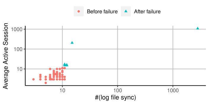
Figure 1. Joint distribution of the Average Active Session (an SLI of the Oracle database) and the number of log file sync waiting events within 2 hours. Each data point represents the two metrics’ values at the same timestamp.

This figure is a scatter plot between the number of log file sync waiting events (x-Axis) and the Average Active Session (AAS for y-Axis) around a high AAS failure. Observed data before the failure are in the bottom-left corner of the figure, while the data after the failure distribute towards the far top-right corner.

We implement the proposed Causal Inference-based Root Cause Analysis (CIRCA). CIRCA outperforms baseline methods in our simulation study, illustrating its theoretical reliability. We further evaluate CIRCA with a real-world dataset. CIRCA improves the recall of the top-1 recommendation by 25% over the best baseline method, which shows the practical potential of our approach. The contributions of this work are summarized as follows.

• For the first time in the literature, we formulate the RCA problem in OSS as a new causal inference task named intervention recognition (Definition 2.1). Utilizing the advance of causal inference, we find a practical criterion to locate the root cause (Theorem 3.4).

• We propose Causal Inference-based Root Cause Analysis (CIRCA) for OSS. We propose a practical guideline to construct the CBN with the knowledge of system architecture. Two more techniques, namely regression-based hypothesis testing and descendant adjustment, are proposed to infer root cause metrics in the graph.

• CIRCA is evaluated with both simulation and real-world datasets. The simulation study illustrates CIRCA’s theoretical reliability, while the real-world dataset shows CIRCA’s practical value over baseline methods.

2. Problem Formulation

2.1. Preliminary

Notation. An upper case letter (e.g., $X$) refers to a variable (metric), while a lower case letter (e.g., $x$) represents an assignment of the corresponding variable. By assignment, we mean one of the possible values. To distinguish variables (values) at different times in a time series, the timestamp will be put on the letter as a superscript. For example, denote AAS as an upper case letter $Y$, and $y^{(t)}$ refers to the value of AAS at time $t$. Denote the value range of $Y$ as $Val(Y)$, then we have $y^{(t)}\in Val(Y)=\{0\}\cup\mathbb{R}^{+}$ for the non-negative numeric AAS. A boldfaced letter means a set of elements (variables or values), e.g., we denote all the metrics as $\mathbf{V}$ while $\mathbf{v}$ is an assignment of $\mathbf{V}$.

The Ladder of Causation. We formulate the problem with Judea Pearl’s “Ladder of Causation” (Bareinboim et al., 2022). The first layer of the causal ladder encodes the observational knowledge $\mathcal{L}_{1}(\mathbf{V})=P(\mathbf{V})$, where $P(\mathbf{V})$ is a joint probability distribution. Meanwhile, the second layer encodes the interventional knowledge $\mathcal{L}_{2}(\mathbf{m})=P_{\mathbf{m}}$, where $P_{\mathbf{m}}(\mathbf{V})=P(\mathbf{V}\mid do(\mathbf{m}))$ and $\mathbf{M}\subseteq\mathbf{V}$. The do-operator $do(\mathbf{m})$ means fixing variables $\mathbf{M}$ to the given values $\mathbf{m}$, also called an intervention (Pearl, 2009). So that $P(\mathbf{V}\mid do(\mathbf{m}))$ indicates the probability distribution over $\mathbf{V}$ under the intervention to $\mathbf{M}$. Finally, the third layer encodes the counterfactual knowledge, reasoning about what if another situation happened in the past. For example, it requires the counterfactual knowledge to predict the latency with sufficient computing resources when high latency and full CPU usage are observed. The hierarchy of the causal ladder almost never collapses (named CHT, Causal Hierarchy Theorem (Bareinboim et al., 2022)). If we want to answer the question at Layer i, we need knowledge at Layer i or higher (Bareinboim et al., 2022).

Structural Causal Model (SCM). We model the relations among metrics via the structural causal model (Pearl, 2009). An SCM contains a set of structural equations shown in Eq. (1), where $V_{i}\in\mathbf{V}$ and $\mathbf{Pa}(V_{i})\subseteq\mathbf{V}$. Eq. (1) contains two kinds of parameters: 1) assignments of observed variables $\mathbf{Pa}(V_{i})$, named parents (direct causes) of $V_{i}$, and 2) assignments of unobserved variables $\mathbf{U}_{i}$, where $\mathbf{U}_{i}\cap\mathbf{V}=\emptyset$.

(1) $$v_{i}=f_{i}(\mathbf{pa}(V_{i}),\mathbf{u}_{i})$$

Denote the graph encoded by the SCM as $\mathcal{G}=(\mathbf{V},\mathbf{E})$, where $\mathbf{E}=\{V_{j}\to V_{i}\mid V_{j}\in\mathbf{Pa}(V_{i})\}$ is the set of directed edges. In contrast to $\mathbf{Pa}$, $\mathbf{Ch}(V_{i})=\{V_{j}\mid V_{i}\in\mathbf{Pa}(V_{j})\}$ represents the children of $V_{i}$. This work rests on the following assumptions.

DAG:

$\mathcal{G}$ is a directed acyclic graph (DAG) (Pearl, 2009), following related works in OSS (Chen et al., 2014; Wang et al., 2018; Gan et al., 2021).

Markovian:

“The exogenous parent sets $\mathbf{U}_{i},\mathbf{U}_{j}$ are independent whenever $i\neq j$” (Bareinboim et al., 2022), i.e., $(\forall i\neq j)\mathbf{U}_{i}\perp\!\!\!\perp\mathbf{U}_{j}$, where $\perp\!\!\!\perp$ means independent.

Faithfulness (Pearl, 2009):

Any intervention makes an observable change, i.e., $P(V_{i}\mid\mathbf{pa}(V_{i}),do(v_{i}))\neq P(V_{i}\mid\mathbf{pa}(V_{i}))$.

Under the DAG assumption and the Markovian assumption, $\mathcal{G}$ can be taken as a CBN (Bareinboim et al., 2022).

2.2. Root Cause Analysis and Causal Inference

We set up a concept mapping between the RCA problem and causal inference.

• A fault in OSS is mapped to an unexpected intervention;

• Fault-free data come from the observational distribution;

• Faulty data come from an interventional distribution.

Based on the mapping above, we define a new causal inference task as intervention recognition (Definition 2.1). We formulate RCA discussed in this work as an intervention recognition task in OSS.

Definition 2.1 (Intervention Recognition, IR).

For a given SCM $\mathcal{M}$, let $\mathcal{L}_{1}$ be the observational distribution of $\mathcal{M}$ and $P_{m}=P(\mathbf{V}\mid do(\mathbf{m}))$ be the interventional distribution of a certain intervention $do(\mathbf{m})$. Intervention recognition is to find $\mathbf{m}$ based on $\mathcal{L}_{1}$ and $P_{m}$.

Definition 2.2 (Root Cause).

The root cause is the intervened variables ($\mathbf{M}$). Each element of $\mathbf{M}$ is named a root cause variable.

3. Intervention Recognition Criterion

We argue that IR shall be positioned at the second layer in the ladder of causation, as shown in Theorem 3.1. The proof of Theorem 3.1 is provided in Appendix A. The key to the proof is that IR is the inverse mapping of $\mathcal{L}_{2}$ under the adopted assumptions. Combining Theorem 3.1 with CHT (Bareinboim et al., 2022), we further obtain Corollary 3.2 and 3.3.

Theorem 3.1.

For a given SCM $\mathcal{M}$ with a CBN $\mathcal{G}$, the knowledge of IR for $\mathcal{M}$ is equivalent to $\mathcal{L}_{2}$ under the Faithfulness assumption.

Corollary 3.2.

We need the knowledge at Layer 2 (interventional) to conduct IR.

Corollary 3.3.

The knowledge at Layer 3 (counterfactual) is not necessary to conduct IR.

Hence, we propose to take full advantage of the CBN, as the CBN is a known bridge between observational data and interventional knowledge (Bareinboim et al., 2022). We argue that Theorem 3.4 is a necessary and sufficient condition for a variable to be intervened. The proof of Theorem 3.4 is provided in Appendix B. Based on our concept mapping between RCA and causal inference, the Theorem 3.4 (Intervention Recognition Criterion). is also a criterion to find root cause indicators.

Theorem 3.4 (Intervention Recognition Criterion).

Let $\mathcal{G}$ be a CBN and $\mathbf{Pa}(V_{i})$ be the parents of $V_{i}$ in $\mathcal{G}$. Under the Faithfulness assumption, $V_{i}$ is intervened iff $V_{i}$ no longer follows the distribution defined by $\mathbf{pa}(V_{i})$, i.e.,

$$V_{i}\in\mathbf{M}\Leftrightarrow P_{\mathbf{m}}(V_{i}\mid\mathbf{pa}(V_{i}))\neq\mathcal{L}_{1}(V_{i}\mid\mathbf{pa}(V_{i}))$$

4. Causal Inference-Based Root Cause Analysis

In this section, we propose a novel method named CIRCA. We first present a structural way to determine the parents $\mathbf{Pa}(V_{i})$ for each metric $V_{i}$ based on system architecture. CIRCA adopts regression-based hypothesis testing (RHT) to deal with the incomplete distribution of faulty data. To address the challenge of the incomplete distribution of fault-free data, CIRCA adjusts the anomaly score for suspicious metrics based on their descendants in the CBN.

4.1. Structural Graph Construction

We propose the structural graph (SG) as the CBN for OSS. SG combines the system architecture knowledge with a set of assumptions, which may not suit domains other than OSS. We first classify monitoring metrics into four dimensions, named meta metrics. Several causal assumptions among those four kinds of meta metrics provide the building blocks of an SG. We further extend the system with the architecture of components to construct a graph at the meta metric level, named a skeleton. Finally, we plug monitoring metrics into the corresponding meta metric to obtain the SG. Algorithm 1 summarizes the overall procedure.

4.1.1. Meta Metrics

In general, a service takes input and produces output. Each request lasts for some time and consumes some resources. We take those dimensions as four meta metrics of a service, named after the four golden signals in site reliability engineering (Beyer et al., 2016). Traffic, Errors, and Latency measure the distribution of input, output, and processing time, respectively. We classify other monitoring metrics as resource consumption, denoted as Saturation.

We assign directions for the relations among these four meta metrics in Figure 2(a). As the start of a request, Traffic is assumed to be the cause of all other three meta metrics, while Errors (the end of a request) are taken as the effect of others. The edge from Saturation to Latency encodes our preference on the former, as resource consumption is one of the common considerations for large latency in OSS (Gan et al., 2021).

(a) Causal assumptions within a service

(b) The skeleton of one web service (WEB) with its dependent database (DB). We plug DB’s meta metrics into the Saturation of WEB.

Figure 2. Causal assumptions among meta metrics

Traffic is assumed as the cause of Saturation, Latency, and Errors. Saturation is assumed as the cause of Latency and Errors. Latency is assumed as the cause of Errors.

4.1.2. Skeleton with Architecture Extension

A complex OSS system will invoke multiple services to process one single request. Meanwhile, there will be multiple components for monolithic OSS. Based on the architecture knowledge encoded in the call graph, we construct the skeleton among meta metrics of the system and all its dependent services. For a web service (WEB) and its database (DB) shown in Figure 2(b), we take DB as a resource of WEB. The part of WEB’s Saturation that measures DB will be extended into DB’s meta metrics, which inherit the relations between WEB’s Saturation and other meta metrics of WEB. The extension will be applied to each service in the call graph. In summary, we introduce three more causal assumptions between a service and its dependent ones.

• The caller’s Traffic influences the callees’ Traffic;

• The callees’ Latency contributes to the caller’s Latency;

• The caller’s output is calculated based on the callees’ output.

4.1.3. Monitoring Metric Plugging-in

Finally, we plug monitoring metrics in meta metrics to obtain the SG. A mapping is required to describe which dimension of which service each monitoring metric measures. There can be some meta metrics that do not have any monitoring metrics. For example, the common measurement for memory is just usage (Traffic), while the speed (Latency) is unavailable. Moreover, one monitoring metric can be derived from multiple meta metrics. For example, DB access per request is calculated by the Traffic of both a web service and a database.

Algorithm 1 describes the plugging-in process after skeleton construction. SG links monitoring metrics from one meta metric to its children (Line 15). Monitoring metrics that are derived from multiple meta metrics may introduce self-loop. To avoid such cycles, the monitoring metric for the last meta metric in topological order will be taken as the common effect of other meta metrics (from Line 6 to Line 14). Moreover, meta metrics measuring the dimension of Errors will be accumulated for descendants (Line 17), as broken data may not be validated in time.

During the process, an empty meta metric will gather the monitoring metrics of its parents for its children (Line 20). Consider a meta metric ($V_{i}^{m}$), one of its parents without monitoring ($V_{j}^{m}$), and their structural equations ($f_{i}^{m}$ and $f_{j}^{m}$). We can substitute $f_{j}^{m}$ for unobserved $V_{j}^{m}$ in $f_{i}^{m}$, as shown in Eq. (2). Both the parents of $V_{j}^{m}$ and those of $V_{i}^{m}$ (except $V_{j}^{m}$) show as the parameters of $f_{i}^{m\prime}$, which is the reason behind Line 20.

(2) $$v_{i}^{m} =f_{i}^{m}\left(f_{j}^{m}\left(\mathbf{pa}_{\mathcal{G}_{skel}}(V_{j}^{m}),\mathbf{u}_{j}^{m}\right),\mathbf{pa}_{\mathcal{G}_{skel}}(V_{i}^{m})\setminus\{v_{j}^{m}\},\mathbf{u}_{i}^{m}\right)$$

$$=f_{i}^{m\prime}\left(\mathbf{pa}_{\mathcal{G}_{skel}}(V_{j}^{m}),\mathbf{pa}_{\mathcal{G}_{skel}}(V_{i}^{m})\setminus\{v_{j}^{m}\},\mathbf{u}_{i}^{m},\mathbf{u}_{j}^{m}\right)$$

Algorithm 1 Structural Graph Construction

0:  $\mathcal{G}_{c}$, the call graph; $\mathbf{h}:\mathbf{V}^{m}\to 2^{\mathbf{V}}$, the mapping from meta metrics $\mathbf{V}^{m}$ to monitoring metrics

1:  $\mathcal{G}_{s}\leftarrow$ initial the structure graph

2:  $\mathcal{G}_{skel}\leftarrow$ construct the skeleton based on $\mathcal{G}_{c}$

3:  for all $V_{i}^{m}\in\mathbf{V}^{m}$ in a topological order from $\{V_{j}^{m}\mid\lvert\mathbf{Pa}_{\mathcal{G}_{skel}}(V_{j}^{m})\rvert=0\}$ do

4:     $\mathbf{Q}_{i}\leftarrow$ Collect monitoring metrics of $\mathbf{Pa}_{\mathcal{G}_{skel}}(V_{j}^{m})$

5:     $\mathbf{C}_{i}\leftarrow$ Collect monitoring metrics of $V_{i}^{m}$

6:     for $V_{j}\in\mathbf{h}(V_{i}^{m})$ do

7:        if $V_{j}$ is mapped to multiple meta metrics then

8:           $\mathbf{C}_{i}\leftarrow\mathbf{C}_{i}\setminus\{V_{j}\}$ /* Prevent self loop of $V_{j}$ */

9:           if $V_{j}$ is visited for the last time then

10:              Add edges from the corresponding meta metrics of $V_{j}$ other than $V_{i}^{m}$ to $V_{j}$ in $\mathcal{G}_{s}$

11:              $\mathbf{Q}_{i}\leftarrow\mathbf{Q}_{i}\cup\{V_{j}\}$ /* Take it as the proxy of others */

12:           end if

13:        end if

14:     end for /* Deal with monitoring metrics that are derived from multiple meta metrics */

15:     Add edges from $\mathbf{Q}_{i}$ to $\mathbf{C}_{i}$ in $\mathcal{G}_{s}$

16:     if $V_{i}^{m}$ represents Errors then

17:        Update $\mathbf{C}_{i}$ with monitoring metrics from the Errors-representing meta metrics in $\mathbf{Pa}_{\mathcal{G}_{skel}}(V_{j}^{m})$

18:     end if/* Transfer Errors */

19:     if $\mathbf{C}_{i}=\emptyset$ then

20:        $\mathbf{h}(V_{i}^{m})\leftarrow\mathbf{Q}_{i}$ /* Gather monitoring metrics for children */

21:     else

22:        $\mathbf{h}(V_{i}^{m})\leftarrow\mathbf{C}_{i}$

23:     end if

24:  end for

25:  return  $\mathcal{G}_{s}$

4.2. Regression-based Hypothesis Testing

The understanding of $P_{\mathbf{m}}$ is restricted by mitigating the failure as soon as possible. Instead of comparing two distributions directly, we reformulate the Theorem 3.4 (Intervention Recognition Criterion). as hypothesis testing with the following null hypothesis ($\mathbf{H}_{0}$) for each metric $V_{i}$.

$\mathbf{H}_{0}$:

$V_{i}$ is not an indicator of the root cause, i.e.,

$$V_{i}^{(t)}\sim\mathcal{L}_{1}\left(V_{i}^{(t)}\mid\mathbf{pa}^{(t)}(V_{i})\right)$$

We utilize the regression technique to calculate the expected distribution $\mathcal{L}_{1}\left(V_{i}^{(t)}\mid\mathbf{pa}^{(t)}(V_{i})\right)$. A regression model is trained for each variable with data before the fault is detected, performing as a proxy of the corresponding structural equation. Let $\bar{v}_{i}^{(t)}$ be the regression value for $v_{i}^{(t)}$. Assuming that the residuals follow an i.i.d. normal distribution $N(\mu_{\epsilon,i},\sigma_{\epsilon,i})$, Eq. (3) measures to what extent a new datum $v_{i}^{(t)}$ deviates from the expected distribution, denoted as $a_{V_{i}}^{(t)}$. Eq. (4) further aggregates $a_{V_{i}}^{(t)}$ for all the available data during the abnormal period as the anomaly score of $V_{i}$.

(3) $$a_{V_{i}}^{(t)}=\left|\frac{\left(v_{i}^{(t)}-\bar{v}_{i}^{(t)}\right)-\mu_{\epsilon,i}}{\sigma_{\epsilon,i}}\right|$$

(4) $$s_{V_{i}}=\max_{t}a_{V_{i}}^{(t)}$$

4.3. Descendant Adjustment

There will be bias in the regression results due to a poor understanding of $\mathcal{L}_{1}$. We adjust the anomaly score of one metric with those of its descendants. Our intuition is that when both a metric and one of its parents in the CBN is abnormal, we prefer the latter. For example, supplementing extra resources is an actionable mitigation method to restore the low latency. Hence, we assign a higher score for resource utilization (the parents of latency in the CBN) than latency’s score.

We summarize the adjustment in Algorithm 2. The children of a metric $V_{i}$ are first considered (Line 3). We exclude some metrics ($\{V_{i}\mid s_{V_{i}}<3\}$) from the root cause indicators, so called the three-sigma rule of thumb. As the failure propagates through them, those metrics will gather anomaly scores from children for the candidate root cause in their ancestors (Line 6). Finally, the anomaly score of $V_{i}$ ($s_{V_{i}}$) will increase by the maximum of descendants’ scores just mentioned (Line 12).

Algorithm 2 Descendant Adjustment

0:  $\mathbf{s}$, anomaly scores by Eq. (4)

1:  $S\leftarrow$ a mapping from $V_{i}$ to the anomaly scores $S(V_{i})$ that may be the direct effect of $V_{i}$

2:  for $V_{i}\in\mathbf{V}$ in a topological order from $\{V_{j}\mid\lvert\mathbf{Ch}(V_{j})\rvert=0$} do

3:     $S(V_{i})\leftarrow\{s_{V_{j}}\mid V_{j}\in\mathbf{Ch}(V_{i})\}$

4:     for $V_{j}\in\mathbf{Ch}(V_{i})$ do

5:        if $s_{V_{j}}<3$ then

6:           $S(V_{i})\leftarrow S(V_{i})\cup S(V_{j})$

7:        end if

8:     end for

9:  end for/* Collect direct effects */

10:  for $V_{i}\in\mathbf{V}$ do

11:     if $s_{V_{j}}\geq 3$ then

12:        $s_{V_{i}}^{\prime}\leftarrow s_{V_{i}}+\max(S(V_{i}))$ /* Adjust based on descendants */

13:     end if

14:  end for

15:  return  $\mathbf{s}^{\prime}$, the adjusted anomaly scores

5. Experiments

In this section, we compare the performance of different methods. We first conduct a simulation study to verify their theoretical reliability. The effectiveness is further evaluated on a real-world dataset. All the execution duration is measured on a server with an Intel Xeon E5-2620 CPU @ 2.40GHz (22 cores) and 57GB RAM. We release our code at https://github.com/NetManAIOps/CIRCA. More experiment details are in Appendix C.

5.1. Experimental Setup

5.1.1. Hyperparameters

The shortest sampling interval in our real-world dataset is one minute. Due to the performance consideration, finer monitoring resolution for each metric is uncommon in OSS. Thus, different time series will be pre-processed for the same set of timestamps with the same interval of one minute.

For each fault, let $t_{d}$ be the time a fault is detected. We assume that RCA is invoked at $t_{d}+t_{delay}$ to collect necessary information, while it takes data in the period $[t_{d}-t_{ref},t_{d}+t_{delay}]$ for reference. The data in $(t_{d}+t_{delay}-t_{test},t_{d}+t_{delay}]$ are treated as from $P_{\mathbf{m}}$ while $[t_{d}-t_{ref},t_{d}-t_{test}]$ are taken as fault-free. By default, we use $t_{delay}=5$ min, $t_{ref}=120$ min, and $t_{test}=10$ min in the experiments. The effects of different $t_{delay}$ and $t_{ref}$ will be explored in Section 5.4.1 with the real-world dataset. In the rest of this section, we name a fault with its corresponding data in $[t_{d}-t_{ref},t_{d}+t_{delay}]$ as a case.

5.1.2. Evaluation Metrics

Following existing works (Wang et al., 2018; Meng et al., 2020; Yu et al., 2021), we evaluate the performance of a method through the recall with the top-k results, denoted as $AC@k$. Eq. (5) shows the definition of $AC@k$, where $\mathcal{F}$ is a set of faults and $R_{i}(\mathbf{M})$ is the $i$-th result recommended by the method for each fault $\mathbf{M}$. Eq. (5) is slightly different from the evaluation metrics in the previous works (Wang et al., 2018; Meng et al., 2020; Yu et al., 2021), ensuring that $AC@k$ is monotonically non-decreasing with $k$. 73% of developers only consider the top-5 results of a fault localization technique, according to the survey in (Kochhar et al., 2016). As a result, we present $AC@k$ for $k\leq K=5$. Moreover, we show the overall performance by $Avg@K=\frac{1}{K}\sum_{k=1}^{K}AC@k$. In terms of efficiency, we record analysis duration per fault, denoted as $T$ in the unit of seconds.

(5) $$AC@k=\frac{1}{|\mathcal{F}|}\sum_{\mathbf{M}\in\mathcal{F}}\frac{|\mathbf{M}\cap\{R_{i}(\mathbf{M})\mid i=1,2,\cdots,k\}|}{\lvert\mathbf{M}\rvert}$$

5.1.3. Baselines

Each baseline is separated into two steps, namely graph construction and scoring. Monitoring metrics will be ranked based on the scores calculated in the final step. We classify the scoring step in the recent RCA literature for OSS into three groups: DFS-based, random walk-based, and invariant network-based. In each group, we choose the representative works. Moreover, we choose the graph construction methods adopted in those works as the baseline ones for the first step.

In the graph construction step, the PC algorithm (Kalisch et al., 2012) is widely used (Chen et al., 2014; Lin et al., 2018; Wang et al., 2018; Ma et al., 2020). We choose Fisher’s z-transformation of the partial correlation and $G^{2}$ test as the conditional independence tests for PC, denoted as PC-gauss and PC-gsq, respectively. PCMCI (Runge et al., 2019) adapts PC for time series, based on which PCTS (Meng et al., 2020) transfers the lagged graph into the one among monitoring metrics. Moreover, the structural graph proposed in this work is denoted as Structural.

As for the scoring step, DFS traverses the abnormal nodes in the graph, ranking the roots of the sub-graph via anomaly scores (Chen et al., 2014). Its variant DFS-MS further ranks candidate metrics according to correlation with the SLI (Lin et al., 2018). Another variant DFS-MH traverses the abnormal sub-graph until a node is not correlated with its parents (Liu et al., 2021). The DFS-based methods take the result of anomaly detection as input. We choose z-score used in (Lin et al., 2018) and SPOT (Siffer et al., 2017) used in (Meng et al., 2020) as options. These anomaly detection methods are also taken as baselines, denoted as NSigma and SPOT, respectively. Another line of works is random walk-based methods. RW-Par calculates the transition probability via partial correlation (Meng et al., 2020), while RW-2 is short for the second-order random walk with Pearson correlation (Wang et al., 2018). ENMF constructs an invariant network based on the ARX model, explicitly modeling the fault propagation (Cheng et al., 2016). CRD further extends ENMF with broken cluster identification (Ni et al., 2017).

5.2. Simulation Study

Three datasets are generated with 50 / 100 / 500 nodes and 100 / 500 / 5,000 edges, respectively, denoted as $\mathcal{D}_{Sim}^{N}$ where $N$ is the number of nodes. For each dataset, we generate 10 graphs and 100 cases per graph. Evaluation metrics averaged among the 10 graphs will be presented. The parameters of baseline methods are selected to achieve the best AC@5 on the first graph in $\mathcal{D}_{Sim}^{50}$.

5.2.1. Data Generation

We generate time series based on the Vector Auto-regression model, as shown in Eq. (6). $\mathbf{x}^{(t)}$ is a column vector of the metrics at time $t$. $\mathbf{A}$ is the weighted adjacent matrix encoding the CBN. $A_{ij}\neq 0$ means the $j$-th metric is a cause of the $i$-th one, where $A_{ij}$ represents the causal effect, e.g., the memory usage per request. The CBN is enforced to be a connected DAG with only the first node (SLI) having no children. The item $\beta\mathbf{x}^{(t-1)}$ reflects the auto-regression nature of the time series. The final item $\mathbf{\epsilon}^{(t)}$ is Gaussian noises, representing the natural fluctuation due to unobserved variables.

(6) $$\mathbf{x}^{(t)}=\mathbf{A}\mathbf{x}^{(t)}+\beta\mathbf{x}^{(t-1)}+\mathbf{\epsilon}^{(t)}$$

To inject a fault $\mathbf{M}$ at time $t$, we first generate the number of root cause metrics $|\mathbf{M}|$. $|\mathbf{M}|-1$ follows a Poisson distribution, as it is rare for a fault to affect many metrics directly. For each $V_{i}\in\mathbf{M}$, the noise item will be altered as $u_{i}^{(t)}=\epsilon_{i}^{(t)}+a_{i}\sigma_{i}$ for 2 timestamps. The random parameter $a_{i}$ will make the SLI metric abnormal according to the three-sigma rule of thumb.

5.2.2. Performance Evaluation

Table 1 summarizes the performance of different methods in three simulation datasets. The scoring step of each method uses the graph deduced by $\mathbf{A}$ directly, i.e., $X_{j}\in\mathbf{Pa}(X_{i})\Leftrightarrow\mathbf{A}_{ij}\neq 0$. We choose the linear regression for RHT. Moreover, RHT could achieve the best performance in theory if it regards the parents as $\mathbf{Pa}(X_{i}^{(t)})=\mathbf{Pa}^{(t)}(X_{i})\cup\left\{X_{i}^{(t-1)}\right\}$. Such implementation is denoted as RHT-PG, where PG represents the perfect graph. As the linear relation with the perfect graph performs as the best proxy of $\mathcal{L}_{1}$, we do not consider the descendant adjustment in the simulation study.

RHT-PG approaches the ideal performance, outperforming baseline methods ($p<0.001$ in t-test for AC@k), which shows the theoretical reliability of our method. There is a gap between the performance of RHT and RHT-PG, which enlarges as the number of nodes increases. This phenomenon illustrates the restriction of Corollary 3.2 that a broken CBN cannot guarantee a correct answer to RCA. On the other hand, RHT-PG is not perfect yet, which may be the result of statistical errors introduced in hypothesis testing with limited faulty data.

Table 1. Performance of different methods in the simulation study. We put the standard deviation in the parentheses behind each evaluation metric. RHT-PG represents RHT with the perfect graph.

Scoring Method	$\mathcal{D}_{Sim}^{50}$			$\mathcal{D}_{Sim}^{100}$			$\mathcal{D}_{Sim}^{500}$
	AC@1	AC@5	T (s)	AC@1	AC@5	T (s)	AC@1	AC@5	T (s)
NSigma	0.432(0.05)	0.733(0.03)	0.306(0.00)	0.384(0.05)	0.613(0.03)	0.575(0.01)	0.376(0.04)	0.579(0.03)	2.759(0.03)
SPOT	0.508(0.04)	0.761(0.03)	6.601(0.21)	0.451(0.04)	0.670(0.03)	17.365(1.14)	0.225(0.07)	0.509(0.07)	83.465(10.85)
DFS	0.541(0.04)	0.682(0.05)	0.308(0.00)	0.555(0.03)	0.653(0.03)	0.579(0.01)	0.540(0.03)	0.611(0.02)	2.790(0.06)
DFS-MS	0.515(0.03)	0.682(0.05)	0.502(0.00)	0.517(0.03)	0.652(0.03)	0.964(0.01)	0.191(0.09)	0.542(0.06)	4.665(0.06)
DFS-MH	0.178(0.08)	0.217(0.09)	0.501(0.00)	0.272(0.05)	0.365(0.05)	0.969(0.01)	0.489(0.04)	0.605(0.03)	4.735(0.05)
RW-Par	0.188(0.06)	0.433(0.07)	0.714(0.00)	0.136(0.05)	0.295(0.07)	1.761(0.01)	0.004(0.01)	0.017(0.02)	20.246(0.10)
RW-2	0.188(0.06)	0.433(0.07)	0.437(0.00)	0.136(0.05)	0.295(0.07)	1.059(0.01)	0.004(0.01)	0.017(0.02)	10.141(0.11)
ENMF	0.116(0.03)	0.278(0.04)	0.624(0.01)	0.200(0.03)	0.336(0.05)	1.865(0.03)	0.217(0.04)	0.354(0.07)	34.082(0.55)
CRD	0.074(0.02)	0.223(0.04)	4.844(0.03)	0.013(0.01)	0.064(0.02)	6.767(0.10)	0.003(0.01)	0.011(0.01)	46.933(0.74)
RHT	0.598(0.03)	0.880(0.02)	0.338(0.01)	0.535(0.06)	0.749(0.06)	0.658(0.01)	0.510(0.04)	0.644(0.04)	3.326(0.06)
RHT-PG	0.615(0.02)	0.952(0.01)	0.346(0.00)	0.631(0.02)	0.930(0.01)	0.665(0.01)	0.623(0.03)	0.823(0.03)	3.310(0.07)
Ideal	0.617(0.02)	0.999(0.00)		0.633(0.02)	0.999(0.00)		0.634(0.04)	1.000(0.00)

5.2.3. Robustness Evaluation

Faults with the same strength may have different effects on the SLI. Yang et al. name such a phenomenon as the dependency intensity in cloud systems, i.e., “how much the status of the callee service influences the caller service” (Yang et al., 2021). In this simulation study, we further classify faults into three types based on their dependency intensities with the SLI. We evaluate the performance of RCA methods against faults of each type separately.

Eq. (6) can be transformed into $\mathbf{x}^{(t)}=\mathbf{W}(\beta\mathbf{x}^{(t-1)}+\mathbf{\epsilon}^{(t)})$, where $\mathbf{W}=(I-\mathbf{A})^{-1}$. Notice that $\mathbf{W}$ is well-defined as $\mathbf{A}$ is generated to be a DAG, which does not have full rank. The element of $\mathbf{W}$ means that $x_{i}$ will increase by $\mathbf{W}_{ij}$ when $x_{j}$ increases by 1. Denote the standard deviation of $X_{i}$ based on data before fault as $\hat{\sigma}_{i}$. We classify each fault $\mathbf{M}$ in the simulated datasets into three types:

Weak:

The root cause metrics deviate from the normal status dramatically to make a slight fluctuation in the SLI (the first node), i.e., $\left(\forall X_{i}\in\mathbf{M}\right)\mathbf{W}_{1i}\hat{\sigma}_{i}/\hat{\sigma}_{1}<1$;

Strong:

A slight fluctuation in the root cause metrics can change the SLI dramatically, i.e., $\left(\forall X_{i}\in\mathbf{M}\right)\mathbf{W}_{1i}\hat{\sigma}_{i}/\hat{\sigma}_{1}>1$;

Mixed:

A fault contains metrics with both the above two types or $X_{i}$ with $\mathbf{W}_{1i}\hat{\sigma}_{i}/\hat{\sigma}_{1}=1$.

Table 2 shows the results on $\mathcal{D}_{Sim}^{50}$. The results on $\mathcal{D}_{Sim}^{100}$ and $\mathcal{D}_{Sim}^{500}$ are omitted since there are only 4 and 5 strong faults in these two datasets, respectively. RHT and RHT-PG achieve the best results no matter the type of faults, implying that RHT is more robust than baseline methods. Anomaly detection methods have competitive performance with weak faults. Their performance drops in strong faults because root cause metrics may be less abnormal than others. DFS-based methods are sensitive to the results of anomaly detection. Their performance shares a similar trend with anomaly detection methods, from weak faults to strong ones.

Table 2. Robustness evaluation on $\mathcal{D}_{Sim}^{50}$. Faults are classified into three types based on their indicators’ influence on SLI.

Scoring Method	Weak (n=916)		Mixed (n=64)		Strong (n=20)
	AC@1	AC@5	AC@1	AC@5	AC@1	AC@5
NSigma	0.454	0.753	0.249	0.498	0.000	0.550
SPOT	0.534	0.783	0.293	0.503	0.000	0.550
DFS	0.558	0.707	0.282	0.368	0.550	0.550
DFS-MS	0.531	0.707	0.277	0.368	0.550	0.550
DFS-MH	0.184	0.223	0.069	0.123	0.250	0.250
RW-Par	0.194	0.445	0.142	0.300	0.050	0.300
RW-24	0.194	0.445	0.142	0.300	0.050	0.300
ENMF	0.111	0.269	0.124	0.321	0.300	0.550
CRD	0.071	0.207	0.088	0.353	0.150	0.550
RHT	0.613	0.888	0.325	0.730	0.800	1.000
RHT-PG	0.624	0.954	0.358	0.914	1.000	1.000
Ideal	0.627	1.000	0.358	0.995	1.000	1.000

5.3. Empirical Study on Oracle Database Data

We further evaluate different methods in a real-world dataset, denoted as $\mathcal{D}_{O}$. There are 99 cases in $\mathcal{D}_{O}$. Each case comes from Oracle databases with high AAS faults in a large banking system. We choose the parameters of baseline methods for better AC@5.

5.3.1. Implementation

We manually extract the call graph in an Oracle database instance from the official documentation. After that, we map 197 monitoring metrics to meta metrics in the skeleton. The final structural graph contains 2,641 edges. Oracle database instances may have different sets of metrics. Therefore, we construct the structural graph for each instance with monitored metrics.

In this empirical study, the ground truth graph is unavailable. Hence, we compare graph construction methods for each scoring method, choosing the graph with the highest AC@5. Meanwhile, there is no perfect proxy of $\mathcal{L}_{1}$ (like the CBN and linear relation in the simulation study). As a result, we fail to include the ideal implementation of RHT (RHT-PG) in the experiment. We choose the Support Vector Regression (SVR) as the regression method for RHT, which will be discussed in Appendix C.4. To alleviate the bias in hypothesis testing, we equip RHT with the descendant adjustment, denoted as CIRCA.

5.3.2. Performance Evaluation

CIRCA achieves the best results compared with baseline methods, as shown in Table 3. Random walk-based methods achieve their best performance with PCTS while taking much time to construct the graph. With the structural graph, DFS-based methods and CIRCA recommend root cause metrics within seconds.

Table 3. Performance of different methods on $\mathcal{D}_{O}$

Scoring Method	Graph Method	AC@1	AC@5	Avg@5	T (s)
NSigma	Empty	0.323	0.662	0.525	0.472
SPOT	Empty	0.152	0.419	0.296	5.027
DFS	Structural	0.187	0.313	0.271	0.483
DFS-MS	Structural	0.207	0.308	0.275	0.839
DFS-MH	Structural	0.268	0.439	0.372	0.844
RW-Par	PCTS	0.086	0.449	0.290	24.695
RW-24	PCTS	0.086	0.449	0.290	24.559
ENMF	Empty	0.111	0.374	0.254	0.771
CRD	Empty	0.035	0.313	0.165	4.787
CIRCA	Structural	0.404	0.763	0.603	0.578
Ideal		0.929	1.000	0.986

We remove components from CIRCA progressively to show their contribution, summarized in Table 4. The result illustrates that both regression-based hypothesis testing and descendant adjustment have a positive effect. Figure 3 compares the proposed structural graph with other graph construction baselines. We exclude anomaly detection and invariant network-based methods from this figure, as they cannot utilize the CBN. Each box in Figure 3 presents the distribution of AC@5 for a scoring method with different parameters. One data point is the best AC@5 from different graph construction parameters with the same scoring ones. The 3 horizontal lines of each box show 25th, 50th, and 75th percentile, while two whiskers extend to minimum and maximum. The proposed structural graph improves AC@5 for DFS-based methods and CIRCA, while PCTS fits random walk-based methods better.

Table 4. Contribution of CIRCA’s components on $\mathcal{D}_{O}$ with the structural graph.

Scoring Method	AC@1	AC@3	AC@5	Avg@5	T (s)
NSigma	0.323	0.586	0.662	0.525	0.472
RHT	0.328	0.601	0.677	0.546	0.576
CIRCA	0.404	0.616	0.763	0.603	0.578

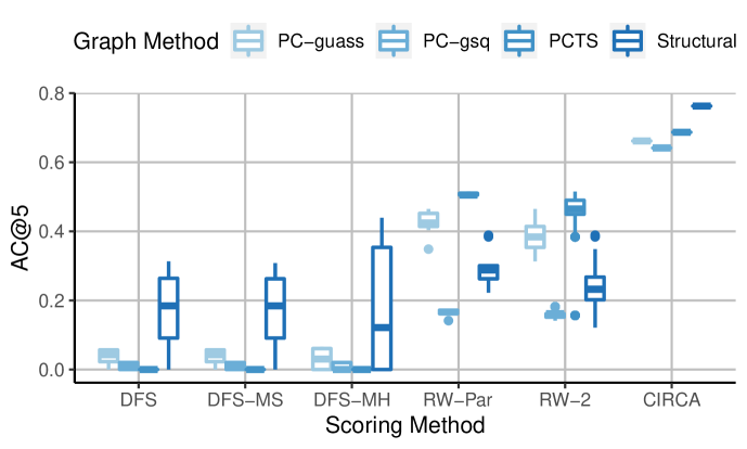
Figure 3. AC@5 for different combinations of ranking methods and graph construction ones

This is a box plot for the combination of ranking methods and graph construction methods. The boxes for DFS-based methods with PC-gsq or PCTS have AC@5 of zero, while the boxes for DFS-based methods with the proposed structural graph are higher than those with PC-gauss. As for random walk-based ranking methods, the boxes with PCTS are higher than other graph construction methods.

5.3.3. Case Study

Figure 4 presents a failure, where “log file sync” (LFS) is the root cause metric labeled by the database administrators (DBAs). A poor understanding of $\mathcal{L}_{1}$ puzzles RCA methods. On the one hand, DFS fails to stop at LFS and continues to check “execution per second” (EPS), missing the desired answer. No baseline method recommends LFS in the top-5 results, except NSigma, ENMF, and CRD. On the other hand, CIRCA assigns a high anomaly score for AAS after revising it from 532.4 (given by NSigma) to 480.2 with regression.

DFS-based methods will drop descendants once meeting an abnormal metric. In contrast, CIRCA scores each metric separately, preventing missing answers like DFS-based methods. Moreover, CIRCA adjusts the anomaly score of LFS with that of the average time of “log file parallel write” (LFPW), i.e., $s_{LFS}^{\prime}=7028.6$. This technique helps CIRCA rank LFS ahead of the other metrics.

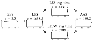
Figure 4. Part of an Oracle database failure, where LFS is the root cause metric labeled by the DBAs. Below each metric name is the score calculated by Eq. (4) and the time series at the same period. Time (horizontal axis) is shown in minutes.

This figure shows part of an Oracle database failure. LFS is the root cause metric. One of its parent, EPS, has an anomaly score slightly larger than 3. On the other hand, the anomaly scores of LFS and its descendants are higher than 480.

5.3.4. Lessons Learned

CIRCA outperforms baseline methods on $\mathcal{D}_{O}$, consistent with the simulation study. Table 4 and Figure 3 further illustrate that each of the 3 proposed techniques has a positive effect.

Though RCA is a difficult task related to Layer 2 of the causal ladder (Corollary 3.2), the knowledge of Layer 1 ($\mathcal{L}_{1}$) is incomplete. We illustrate the negative effect through a case study. We believe that further advancement in the future has to handle this obstacle explicitly. At present, we prefer CIRCA to pure RHT if deployed. Meanwhile, the effectiveness of the descendant adjustment has to be verified on more real-world datasets.

5.4. Discussion

5.4.1. Hyperparameter Sensitivity

Figure 5 compares RCA methods with different $t_{delay}$ and $t_{ref}$. CIRCA has stable performance with these two hyperparameters, outperforming baseline methods.

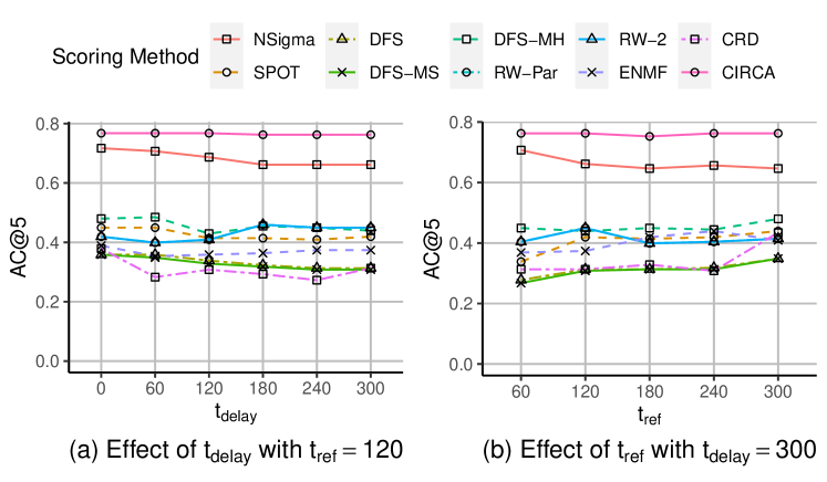
Figure 5. Performance with various hyperparameters on $\mathcal{D}_{O}$

There are two line charts, showing the performance of baseline methods with different hyperparameters. The left one fixes $t_{ref}=120$, varying $t_{d}elay$, while the right one fixes $t_{delay}=300$, varying $t_{r}ef$.

5.4.2. Performance of Existing Methods

RW-Par and RW-2 represent the scoring methods of MicroCause (Meng et al., 2020) and CloudRanger (Wang et al., 2018), respectively. However, RW-Par (RW-2) fails to achieve the performance in the corresponding paper. MicroCause utilizes metric priority provided by operators, which is unavailable for RW-Par. On the other hand, CloudRanger achieves its best result with a sampling interval of 5 seconds. The coarse monitoring frequency of $\mathcal{D}_{O}$ may explain the poor performance of RW-2.

As stated by Corollary 3.2, knowledge of Layer 2 (such as $\mathbf{Pa}$) is necessary for RCA. The invariant network-based methods utilize the observation data only (Layer 1). Their unsatisfying performance illustrates the restriction of CHT (Bareinboim et al., 2022).

5.4.3. Feasibility

Graph Construction. The construction of the proposed structural graph requires system architecture and a mapping from monitoring metrics to the targets to be monitored. The former is usually in the form of documentation. We argue that a metric is neither insightful nor actionable unless operators understand its underlying meaning. Operators need to classify each distinct metrics only once to obtain the mapping. The mapping can be shared among similar instances of the same type (like Oracle database instances).

Scalability. As shown in Table 1, RHT’s time cost grows around linearly with the size of the dataset. Moreover, the design of CIRCA supports horizontal scalability to handle large-scale systems via adding computing resources, as each metric is scored separately. We plan to train the regression models offline to speed up online analysis. Mature parallel programming frameworks, such as Apache Spark, may further help accelerate CIRCA.

6. Related Works

Root Cause Analysis. Corollary 3.2 explains that graph construction is a common step in the RCA literature for online service system operation. DFS-based methods (Chen et al., 2014; Lin et al., 2018; Liu et al., 2021) traverse abnormal sub-graph, which is sensitive to anomaly detection results. Some works adopt random walk (Wang et al., 2018; Meng et al., 2020; Ma et al., 2020) or PageRank (Wang et al., 2021) to score candidate root cause indicators, lacking explainability. Another line of works is invariant network-based methods (Cheng et al., 2016; Ni et al., 2017). As these works adopt the pair-wise manner to learn the invariant relations, it is hard for them to reach the knowledge of RCA, restricted by CHT (Bareinboim et al., 2022). No methods above utilize causal inference. Sage (Gan et al., 2021) conducts counterfactual analysis to locate root causes without a formal formulation. Corollary 3.3 states that counterfactual analysis is unnecessary. Hence, we did not include this method as a baseline. Meanwhile, CHT (Bareinboim et al., 2022) indicates that it can be hard to conduct counterfactual analysis even with a CBN.

The definition of root cause analysis varies with the scenario in the literature. Some applications require an answer beyond the data, taking RCA as a classification task with supervised learning (Yi and Park, 2021). For homogeneous devices or services, operators are interested in the common features (Zhang et al., 2021). Accordingly, a multi-dimensional root cause analysis is conducted. In contrast, we treat the observed projection of a fault as the desired answer. The Theorem 3.4 (Intervention Recognition Criterion). further relates RCA in this work with contextual anomaly detection (Chandola et al., 2009), treating parents in the CBN as the context for each variable. We take complex contextual anomaly detection methods as future work.

Causal Discovery. The task to obtain the CBN is named causal discovery. We refer the readers to a recent survey (Guo et al., 2020) for a thorough discussion. NOTEARS (Zheng et al., 2018) converts the DAG search problem from the discrete space into a continuous one. Following NOTEARS, some recent works are based on gradient descent (He et al., 2021).

Although causal discovery has its sound theory, the CBN discovered from data directly is not explainable for human operators. In contrast, some works obtain the CBN based on domain knowledge. MicroHECL (Liu et al., 2021) traces the fault along with traffic, latency, or error rate in the call graph. Meanwhile, Sage (Gan et al., 2021) constructs the CBN among latency and machine metrics. The structural graph proposed in this work is compatible with the assumptions in these two works, extending the kinds of meta metrics.

7. Conclusion and Future Work

Root cause analysis (RCA) is an essential task for OSS operations. In this work, we formulate RCA as a new causal inference task named intervention recognition, based on which, we further obtain the Theorem 3.4 (Intervention Recognition Criterion). to find the root cause. We believe such a formulation bridge two well-studied fields (RCA and causal inference) and provide a promising new direction for the critical-yet-hard-to-solve RCA problem in OSS.

To apply such a criterion in OSS, we propose a novel causal inference-based RCA method, CIRCA. CIRCA consists of three techniques, namely structural graph construction, regression-based hypothesis testing, and descendant adjustment. We verify the theoretical reliability of CIRCA in the simulation study. Moreover, CIRCA also outperforms baseline methods in a real-world dataset.

In the future, we plan to include faulty data for regression. We hope that diverse data can help overcome the limited understanding of the system’s normal status. This work rests on a set of assumptions that a real application may not satisfy. For example, some meta metrics do not have corresponding monitoring metrics in the skeleton we construct for the Oracle database. As a result, they can imply common exogenous parents of the downstream monitoring metrics, violating the Markovian assumption. Explicitly modeling these hidden meta metrics may improve RCA performance. Meanwhile, the retrospect of analysis mistakes may also point to the lack of monitoring. Beyond the analysis framework in this work, discoveries on the underlying mechanism of OSS can also help climb the ladder of causation for the RCA task.

Appendix A Proof of Theorem 3.1

We define identifiable intervention recognition (IIR) as follows:

Definition A.1 (Identifiable Intervention Recognition, IIR).

Identifiable intervention recognition is to find out a set of potential interventions $\{\mathbf{m}^{\prime}\mid\mathcal{L}_{1}(\mathbf{V}\mid do(\mathbf{m}^{\prime}))\equiv P_{\mathbf{m}}\}$ (i.e., identifiable interventions).

With Definition A.1, we have Lemma A.2 and Lemma A.3.

Lemma A.2.

The knowledge of IIR can be derived from $\mathcal{L}_{2}$.

Proof of Lemma A.2.

Denote $\mathcal{C}$ as the equivalence classes defined by $\mathcal{L}_{2}$ among $\mathcal{F}=\bigcup_{\mathbf{M}\in 2^{\mathbf{V}}}Val(\mathbf{M})$, where $\mathcal{F}$ is all possible interventions, including no intervention. For each equivalent class $c\in\mathcal{C}$, $c$ is a set of interventions $[\mathbf{m}]$ which leads to the same distribution over $\mathbf{V}$:

$$[\mathbf{m}]=\{\mathbf{m}^{\prime}\mid\mathcal{L}_{1}(\mathbf{V}\mid do(\mathbf{m}^{\prime}))\equiv P_{\mathbf{m}}\}$$

Denote the distribution of V under $[\mathbf{m}]$ as $\mathcal{L}_{2}^{-1}(P_{\mathbf{m}})=[\mathbf{m}]$. Denote $\mathcal{L}_{2}^{\prime}([\mathbf{m}])=P_{\mathbf{m}}$, where $[\mathbf{m}]\in\mathcal{C}$. For any $\mathbf{m}_{1},\mathbf{m}_{2}\in\mathcal{F}$, we always have:

$$P_{\mathbf{m}_{1}}\equiv P_{\mathbf{m}_{2}}\rightarrow[\mathbf{m}_{1}]=[\mathbf{m}_{2}]$$

Hence, $\mathcal{L}_{2}^{\prime}$ is a one-to-one correspondence and have its inverse mapping, denoted as $\mathcal{L}_{2}^{-1}(P_{\mathbf{m}})=[\mathbf{m}]$.

When an intervention occurs, based on $P_{\mathbf{m}}\in\mathcal{L}_{2}(\mathcal{F})$, $\mathcal{L}_{2}^{-1}(P_{\mathbf{m}})$ is the set of targets of IIR. Hence, the knowledge of IIR can be derived from $\mathcal{L}_{2}$. ∎

Lemma A.3.

The knowledge of IIR encodes $\mathcal{L}_{2}$.

Proof of Lemma A.3.

For any valid $P_{\mathbf{m}}\in\mathcal{L}_{2}(\mathcal{F})$, IIR will produce a set of possible interventions $\{\mathbf{m}^{\prime}\mid\mathcal{L}_{2}(\mathbf{m}^{\prime})\equiv P_{\mathbf{m}}\}$. Hence, the knowledge of IIR can be extended to the mapping $\mathcal{L}_{2}^{-1}$ that maps $P_{\mathbf{m}}$ to the element of $\mathcal{C}$. Meanwhile, $\mathcal{L}_{2}^{-1}$ is the inverse mapping of $\mathcal{L}_{2}^{\prime}$ and $\mathcal{L}_{2}$ can be derived from $\mathcal{L}_{2}^{\prime}$. Hence, the knowledge of IIR encodes $\mathcal{L}_{2}$. ∎

Based on Lemma A.2 and Lemma A.3, the knowledge of IIR is equivalent to $\mathcal{L}_{2}$. Then we have Theorem A.4.

Theorem A.4.

The knowledge of IIR is at the second layer of the causal ladder.

For an SCM with a CBN, we get Lemma A.5.

Lemma A.5.

For a given SCM $\mathcal{M}$ with a CBN $\mathcal{G}$, let $\mathbf{Pa}(V_{i})$ be the parents of $V_{i}$ in $\mathcal{G}$. $P(V_{i}\mid\mathbf{pa}(V_{i}),do(\mathbf{m}))$ can be reduced to the form defined in Eq. (7).

(7) $$P(V_{i}\mid\mathbf{pa}(V_{i}),do(\mathbf{m}))=\left\{\begin{array}[]{ll}P(V_{i}\mid\mathbf{pa}(V_{i}),do(v_{i})),&V_{i}\in\mathbf{M}\\ P(V_{i}\mid\mathbf{pa}(V_{i})),&V_{i}\notin\mathbf{M}\\ \end{array}\right.$$

Proof of Lemma A.5.

Given a variable $V_{i}$, the intervened variables $\mathbf{M}$ can be separated into three parts: 1) $\mathbf{M}_{Pa}=\mathbf{M}\cap\mathbf{Pa}(V_{i})$, 2) $\mathbf{M}_{i}=\mathbf{M}\cap\{V_{i}\}$, and 3) $\mathbf{M}_{Other}=\mathbf{M}\setminus\mathbf{Pa}(V_{i})\setminus\{V_{i}\}$. Hence,

• $\mathbf{M}=\mathbf{M}_{Pa}\cup\mathbf{M}_{i}\cup\mathbf{M}_{Other}$,

• $\mathbf{M}_{Pa}\cap\mathbf{M}_{i}=\mathbf{M}_{Pa}\cap\mathbf{M}_{Other}=\mathbf{M}_{i}\cap\mathbf{M}_{Other}=\emptyset$, and

• there is no arrow from $\mathbf{M}_{Other}$ to $V_{i}$ in $\mathcal{G}$.

Case 1.

With $V_{i}\in\mathbf{M}$, denote the interventional SCM of $\mathcal{M}$ with $do(\mathbf{m})$ as $\mathcal{M}^{\prime}$. $\mathcal{M}^{\prime}$ replaces $f_{i}$ in $\mathcal{M}$ with $v_{i}\leftarrow m_{i}$ (Pearl, 2009). As a result, other variables cannot affect $V_{i}$ any longer. Hence, $do(v_{i})$ makes $P(V_{i}\mid\mathbf{pa}(V_{i}),do(\mathbf{m}))$ and $P(V_{i}\mid\mathbf{pa}(V_{i}),do(v_{i}))$ equivalent by

$$P(V_{i}\mid\mathbf{pa}(V_{i}),do(\mathbf{m}))=P(V_{i}\mid do(v_{i}))=P(V_{i}\mid\mathbf{pa}(V_{i}),do(v_{i}))$$

Case 2.

With $V_{i}\notin\mathbf{M}$, we get $\mathbf{M}_{i}=\emptyset$ and $\mathbf{M}=\mathbf{M}_{Pa}\cup\mathbf{M}_{Other}$ for the equation below

$$P(V_{i}\mid\mathbf{pa}(V_{i}),do(\mathbf{m}))=P(V_{i}\mid\mathbf{pa}(V_{i}),do(\mathbf{m}_{Pa}),do(\mathbf{m}_{Other}))$$

Since $\mathcal{G}$ is a CBN, the “Parents do/see” condition (Bareinboim et al., 2022) states that we can replace $\mathbf{pa}(V_{i})$ with $do(\mathbf{pa}(V_{i}))$.

(8) $$P(V_{i}\mid\mathbf{pa}(V_{i}),do(\mathbf{m}))=P(V_{i}\mid do(\mathbf{pa}(V_{i})),do(\mathbf{m}_{Other}))$$

As we already take $do(\mathbf{m}_{Pa})$ as the condition, the “Missing-link” condition (Bareinboim et al., 2022) ensures that we can drop $do(\mathbf{m}_{Other})$.

(9) $$P(V_{i}\mid\mathbf{pa}(V_{i}),do(\mathbf{m}))=P(V_{i}\mid do(\mathbf{pa}(V_{i})))$$

With the “Parents do/see” condition (Bareinboim et al., 2022) again, we obtain

(10) $$P(V_{i}\mid\mathbf{pa}(V_{i}),do(\mathbf{m}))=P(V_{i}\mid\mathbf{pa}(V_{i}))$$

Combining the two cases above provides the final conclusion. ∎

Proof of Theorem 3.1.

Given an intervention $\mathbf{m}$ and any identifiable intervention $\mathbf{m}^{\prime}$ provided by IIR, $P(\mathbf{V}\mid do(\mathbf{m}))\equiv P(\mathbf{V}\mid do(\mathbf{m}^{\prime}))$. Hence, $P(V_{i}\mid\mathbf{pa}(V_{i}),do(\mathbf{m}))\equiv P(V_{i}\mid\mathbf{pa}(V_{i}),do(\mathbf{m}^{\prime}))$ for any $V_{i}\in\mathbf{V}$. Notice that the corresponding assignment for an intervention is just encoded in the interventional distribution. As a result, $(\forall x\in\mathbf{m},x^{\prime}\in\mathbf{m}^{\prime})X=X^{\prime}\rightarrow x=x^{\prime}$.

Assume that $\mathbf{m}$ is different from $\mathbf{m}^{\prime}$, e.g., $(\exists X\in\mathbf{V})X\in\mathbf{M}\wedge X\notin\mathbf{M}^{\prime}$. With Lemma A.5, we have $P(X\mid\mathbf{pa}(X),do(x))\equiv P(X\mid\mathbf{pa}(X))$, which violates the Faithfulness assumption. It is the same for the case $(\exists X\in\mathbf{V})X\notin\mathbf{M}\wedge X\in\mathbf{M}^{\prime}$. Hence, IIR can distinguish $\mathbf{m}$ from other interventions, providing the same answer as IR.

According to Theorem A.4, we reach the conclusion that the knowledge of IR is at the second layer of the causal ladder. ∎

Appendix B Proof of Theorem 3.4

Proof of Theorem 3.4.

Notice that $P_{\mathbf{m}}(V_{i}\mid\mathbf{pa}(V_{i}))=P(V_{i}\mid\mathbf{pa}(V_{i}),do(\mathbf{m}))$, while $\mathcal{L}_{1}(V_{i}\mid\mathbf{pa}(V_{i}))=P(V_{i}\mid\mathbf{pa}(V_{i}))$.

Case 1.

With $V_{i}\in\mathbf{M}$, we get $\mathbf{M}_{i}=\{V_{i}\}$. Under the Faithfulness assumption, Eq. (11) must hold, while Lemma A.5 provides $P(V_{i}\mid\mathbf{pa}(V_{i}),do(\mathbf{m}))=P(V_{i}\mid\mathbf{pa}(V_{i}),do(v_{i}))$.

(11) $$P(V_{i}\mid\mathbf{pa}(V_{i}),do(v_{i}))\neq P(V_{i}\mid\mathbf{pa}(V_{i}))$$

Hence,

$$V_{i}\in\mathbf{M}\Rightarrow P_{\mathbf{m}}(V_{i}\mid\mathbf{pa}(V_{i}))\neq\mathcal{L}_{1}(V_{i}\mid\mathbf{pa}(V_{i}))$$

Case 2.

With $V_{i}\notin\mathbf{M}$, Lemma A.5 provides $P(V_{i}\mid\mathbf{pa}(V_{i}),do(\mathbf{m}))=P(V_{i}\mid\mathbf{pa}(V_{i}))$. Hence,

$$V_{i}\notin\mathbf{M}\Rightarrow P_{\mathbf{m}}(V_{i}\mid\mathbf{pa}(V_{i}))=\mathcal{L}_{1}(V_{i}\mid\mathbf{pa}(V_{i}))$$

Its contrapositive stands as well,

$$P_{\mathbf{m}}(V_{i}\mid\mathbf{pa}(V_{i}))\neq\mathcal{L}_{1}(V_{i}\mid\mathbf{pa}(V_{i}))\Rightarrow V_{i}\in\mathbf{M}$$

, which is the converse proposition of Case 1.

In conclusion, $V_{i}\in\mathbf{M}\Leftrightarrow P_{\mathbf{m}}(V_{i}\mid\mathbf{pa}(V_{i}))\neq\mathcal{L}_{1}(V_{i}\mid\mathbf{pa}(V_{i}))$. ∎

Appendix C Implementation Details

C.1. Baseline Methods

Most of the code in this work is written in Python, while we adopt the R package pcalg (Kalisch et al., 2012) for the PC algorithm. We utilize process-based parallel programming to isolate errors only.

NSigma calculates $\max_{t}\frac{\lvert v_{i}^{(t)}-\mu_{i}\rvert}{\sigma_{i}}$. We adopt the authors’ implementation for SPOT (Siffer et al., 2017) while re-implementing ENMF (Cheng et al., 2016) in Python based on the authors’ MATLAB implementation. The other baseline methods are not publicly available. We implement them by our understanding.

C.2. Simulation Data Generation

We generate the simulation datasets based on the Vector Auto-regression model, as shown in Eq. (6). Following existing work (Zheng et al., 2018; He et al., 2021), the value of non-zero elements in the weighted adjacent matrix, $A_{ij}$, is uniformly sampled from $(-2.0,-0.5)\cup(0.5,2.0)$. For the second item $\beta\mathbf{x}^{(t-1)}$, we set $\beta=0.1$ in the experiment. Finally, we sample the standard deviations from an exponential distribution for the zero-mean Gaussian noises $\mathbf{\epsilon}^{(t)}$.

The structure of $A$ is generated in two steps, as shown in Algorithm 3. We first generate a tree to ensure that the graph is a connected DAG. Then, the other edges are inserted randomly.

Algorithm 3 Graph Generation in the Simulation Study

0:  $N_{node}$, the number of nodes; $N_{edge}$, the number of edges

1:  $\mathcal{G}\leftarrow(\mathbf{V},\mathbf{E})$, where $\mathbf{V}=\{1,2,\cdots,N_{node}\}$

2:  for $i=2,\cdots,N_{node}$ do

3:     $j\leftarrow$ choose one node from $\{1,2,\cdots,i-1\}$ randomly

4:     Add the edge $i\rightarrow j$ into $\mathbf{E}$

5:  end for

6:  for $k=N_{node},N_{node}+1,\cdots,N_{edge}$ do

7:     $i,j\leftarrow$ sample $i,j\in\mathbf{V}$ randomly, s.t., $i>j\wedge(i\rightarrow j)\notin\mathbf{E}$

8:     Add the edge $i\rightarrow j$ into $\mathbf{E}$

9:  end for

10:  return  $\mathcal{G}$

C.3. Structural Graph Construction

In the empirical study, we construct the structural graph for the Oracle database instances. Figure 6 shows the SQL processing and memory structures in the call graph. Figure 4 further shows part of the graph among metrics. We drop metrics not included in the final structural graph, as our knowledge fails to cover them. Baseline methods only use labeled metrics for a fair comparison.

Figure 6. Part of the Oracle database call graph

This figure shows the Stages of SQL Processing and Memory Structures. We convert the related documentation into such a call graph.

C.4. Regression Method Selection

Table 5 shows RHT’s performance with several regression methods. RHT with the linear regression (Linear) has unsatisfying performance, as the relations among real-world variables are seldom linear. Support Vector Regression (SVR) with the sigmoid kernel, which is non-linear, improves the performance. Fu et al. provide a way to predict distribution based on Random Forest (RF) and Mixture Density Networks (MDN), respectively, instead of a single value (Fu et al., 2021). Hence, RHT combined with RF or MDN can measure the deviation for a new datum against the predicted distribution. However, these two methods perform worse than the simple linear regression due to a limited understanding of the normal status, as shown in Figure 1. As a result, we choose SVR in the empirical study.

Table 5. RHT with different regression methods on $\mathcal{D}_{O}$

Regression Method	AC@1	AC@3	AC@5	Avg@5	T (s)
Linear	0.197	0.424	0.556	0.409	0.559
SVR	0.328	0.601	0.677	0.546	0.834
RF	0.202	0.394	0.525	0.382	22.065
MDN	0.111	0.212	0.253	0.195	694.329