Curvilinearity and Orthogonality

Abstract

We introduce sequences of functions orthogonal on a finite interval: proper orthogonal rational functions, orthogonal exponential functions, orthogonal logarithmic functions, and systems of transmuted orthogonal polynomials.

1 Introduction

General properties of orthogonal rational functions were studied in [2, 14]. Specific examples of orthogonal rational functions on the semi-axis were given in [1, 10, 15]. Alternative orthogonal rational functions on a half-line which provide term-by-term increasing rate of decay at infinity were introduced in [7].

Orthogonal exponential functions on the semi-axis were presented in [11]. Alternative orthogonal exponential functions on the semi-axis with term-by-term increasing rate of decay at infinity were developed in [4, 5, 6].

Orthogonal logarithmic functions with weak singularity at one end of an interval were introduced in [9].

Standard theory of orthogonal polynomials [12] includes statement that zeros of the polynomials are distributed in an orthogonality interval. Alternative orthogonal polynomials [5, 6] have zeros both inside and at one end of an interval. Structured orthogonal polynomials [8] admit zeros inside and at both ends of an interval. One can also introduce orthogonal polynomials that have prescribed zeros outside of an orthogonality interval. Being not of specific interest by itself, such altered orthogonal polynomials may originate orthogonal rational functions and other orthogonal functions on an interval.

In this preliminary notice, we alter Legendre polynomials [13] and use transforms for independent variable $x$ on the $x$-axis to compose sequences of proper orthogonal rational functions on an interval, as well as sequences of orthogonal exponential functions and orthogonal logarithmic functions on an interval.

In addition, we introduce systems of transmuted orthogonal polynomials that have complex zeros and may be another origin for above mentioned compositions.

2 Altered Legendre polynomials

Let $\widetilde{P}_{n}(x)$ be shifted Legendre polynomials. Making use of $\widetilde{P}_{n}(x)$, we introduce polynomials

$$A_{n}(x)=\frac{x+1}{2}\widetilde{P}_{n-1}(x),\quad x\in[-1,1],\quad n=1,2,…$$ (1)

that are orthogonal

$$\int_{0}^{1}\frac{A_{m}(x)A_{n}(x)}{(x+1)^{2}}{\rm d}x=\frac{\delta_{mn}}{4(2n-1)}$$

and have a fixed real zero $x=-1$ outside the interval of orthogonality. Properties of ${A_{n}(x)}$ can be easily derived from definition (1) and properties of Legendre polynomials. Altered Legendre polynomials $A_{n}(x)$ form a basis in $L^{2}[0,1]$, and a polynomial $\widetilde{P}_{k}(x)$ can be approximated by the sequence $A_{n}(x)$ on the interval. In particular, one can find

$$\widetilde{P}_{0}(x)=1\approx 2\ln 2\cdot A_{1}(x)-6(3\ln 2-2)A_{2}(x))+10(13\ln 2-9)A_{3}(x)-...\hskip 3.0pt.$$ (2)

Expansion (2) provides fast convergence for $x\in[0,1]$ and shows good results for extrapolation outside of the interval.

3 Proper orthogonal rational functions on an interval

Making use of Cayley transform [3]

$$x\mapsto\frac{1-x}{1+x}$$ (3)

that maps points $\{-1,0,1\}$ to points $\{\infty,1,0\}$ on the $x$-axis, we define proper Legendre rational functions as a composition

$$R_{n}(x):=(-1)^{n-1}A_{n}\left(\frac{1-x}{1+x}\right),\quad x\in[0,\infty),\quad n=1,2,...\hskip 3.0pt.$$

Functions $R_{n}(x)$ are orthogonal on the interval $[0,1]$, and

$$\int_{0}^{1}R_{m}(x)R_{n}(x){\rm d}x=\frac{\delta_{mn}}{2(2n-1)}.$$

It may be noted that function

$$f(x)=\frac{1-x}{1+x}$$

is an involution, so function $f^{-1}(x)$ provides the same composition as $f(x)$ does.

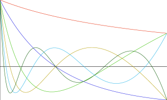
Fig. 1: $R_{n}(x),\hskip 3.0ptn=1-6$.

We find

$$R_{1}(x)=\frac{1}{x+1},$$

$$R_{2}(x)=\frac{1-3x}{(x+1)^{2}},$$

$$R_{3}(x)=\frac{13x^{2}-10x+1}{(x+1)^{3}},$$

$$R_{4}(x)=\frac{(1-3x)(21x^{2}-18x+1)}{(x+1)^{4}},$$

$$R_{5}(x)=\frac{321x^{4}-516x^{3}+246x^{2}-36x+1}{(1+x)^{5}},$$

$$R_{6}(x)=\frac{(1-3x)(1-52x+454x^{2}-948x^{3}+561x^{4})}{(1+x)^{6}},$$

and

$$R_{n}(0)=1,\quad R_{n}(1)=\frac{(-1)^{n-1}}{2},\quad\lim_{x\rightarrow\infty}R_{n}(x)=0.$$

From properties of Legendre polynomials it follows that $R_{n}(x)$ with even indices have a zero at $x=1/3$.

Functions $R_{n}(x)$ form a basis in $L^{2}[0,1]$. In the complex $z$-plain, $R_{n}(z)$ have one $n$-degree pole at $z=-1$.

4 Orthogonal exponential functions on an interval

Making use of a transform of exponential type

$$x\mapsto 2^{1-x}-1$$ (4)

that maps points $\{-1,0,1\}$ to points $\{\infty,1,0\}$ on the $x$-axis, we compose a sequence of Legendre exponential functions

$$E_{n}(x):=(-1)^{n-1}A_{n}(2^{1-x}-1),\quad x\in[0,\infty),\quad n=1,2,...\hskip 3.0pt$$

that obey orthogonality relation

$$\int_{0}^{1}2^{x}E_{m}(x)E_{n}(x){\rm d}x=\frac{\delta_{mn}}{2\ln 2(2n-1)}.$$

For convenience, we introduce polynomial functions $F_{n}(t)$ and specify $E_{n}(x)$ as compositions of $F_{n}(t)$ and an exponential function $t(x)=2^{-x}$, that is,

$$E_{n}(x)\equiv F_{n}(t)_{t=2^{-x}}\quad n=1,2,...\hskip 3.0pt.$$

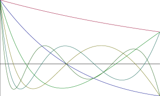
Fig. 2: $E_{n}(x),\hskip 3.0ptn=1-6$.

We find

$$F_{1}(t)=t,$$

$$F_{2}(t)=t(4t-3),$$

$$F_{3}(t)=t(24t^{2}-36t+13),$$

$$F_{4}(t)=t(4t-3)(40t^{2}-60t+21),$$

$$F_{5}(t)=t(1120t^{4}-3360t^{3}+3720t^{2}-1800t+321),$$

$$F_{6}(t)=t(4t-3)(2016t^{4}-6048t^{3}+6664t^{2}-3192t+561),$$

and

$$E_{n}(0)=1,\quad E_{n}(1)=\frac{(-1)^{n-1}}{2},\quad\lim_{x\rightarrow\infty}E_{n}(x)=0.$$

It appears that $E_{n}(x)$ with even indices have a zero at

$$x=2-\ln 3/\ln 2=0.415037499...\hskip 3.0pt.$$ (5)

Functions $E_{n}(x)$ form a basis in $L^{2}[0,1]$.

5 Orthogonal logarithmic functions on an interval

A function

$$g(x)=2^{1-x}-1.$$

is not an involution, but it is a near involution on the interval $[0,1]$. Inverse of $g(x)$ is the function

$$g^{-1}(x)=1-\log_{2}(1+x),$$

and one may find that

$$\left(\int_{0}^{1}(g(x)-g^{-1}(x))^{2}{\rm d}x\right)^{1/2}=0.002719224...\hskip 3.0pt.$$

Also,

$$g(x)=g^{-1}(x)\quad{\rm at}\quad x=0,\quad x=0.456999559...,\quad{\rm and}\quad x=1.$$

Making use of a transform of logarithmic type

$$x\mapsto 1-\log_{2}(1+x)$$ (6)

that maps the points $\{-1,0,1\}$ to $\{3,1,0\}$ on the $x$-axis, we define Legendre logarithmic functions

$$L_{n}(x):=(-1)^{n-1}A_{n}(1-\log_{2}(1+x)),\quad x\in[0,3],\quad n=1,2,...\hskip 3.0pt.$$

Functions $L_{n}(x)$ are orthogonal on the interval $[0,1]$, and

$$\int_{0}^{1}\frac{1}{\frac{1+x}{4}{\rm log}_{2}^{2}\frac{1+x}{4}}L_{m}(x)L_{n}(x){\rm d}x=\frac{\delta_{mn}}{1/\ln 2(2n-1)}.$$

Also, we introduce polynomial functions $G_{n}(t)$ and identify $L_{n}(x)$ as compositions of $G_{n}(t)$ and a logarithmic function $t(x)=\log_{2}(1+x)$,

$$L_{n}(x)\equiv G_{n}(t)_{t=\log_{2}(1+x)}\quad n=1,2,...\hskip 3.0pt.$$

We find

$$G_{n}(t)=(-1)^{n-1}(1-\frac{1}{2}t)\widetilde{P}_{n-1}(t),$$

and

$$L_{n}(0)=1,\quad L_{n}(1)=\frac{(-1)^{n-1}}{2},\quad L_{n}(3)=0.$$

It appears that $L_{n}(x)$ with even indices have a zero at

$$x=\sqrt{2}-1=0.414213562...\hskip 3.0pt.$$ (7)

Numbers in (5) and (7) are “almost the same”. Actually,

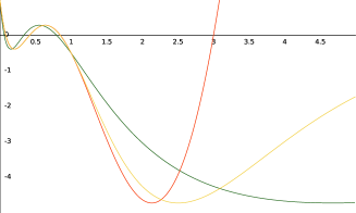
Fig. 3: $R_{4}(x)$ (green), $E_{4}(x)$ (yellow), $L_{4}(x)$ (red).

the graphs of the functions $E_{n}(x)$ and $L_{n}(x)$ are very close on the interval of orthogonality, but they differ outside of the interval.

Functions $L_{n}(x)$ form a basis in $L^{2}[0,1]$.

6 Conjecture

Calculations show that the following statement may take place. Let $r_{nk}$, $e_{nk}$, and $l_{nk}$ be abscissas of local extrema for functions $R_{n}(x)$, $E_{n}(x)$, and $L_{n}(x)$. Then $R_{n}(r_{nk})=E_{n}(e_{nk})=L_{n}(l_{nk})$.

7 Conclusion

Altered Legendre polynomials ${A}_{n}(x)$ originate three sequences of orthogonal functions, $R_{n}(x)$, $E_{n}(x)$, and $L_{n}(x)$.

The sequences are bases for approximation in $L^{2}[0,1]$ space, and they may provide spectral convergence properties. One may notice that a linear function $s(x)=ax+b$ cannot be represented exactly by a finite linear combination of any of the three sequences, and the bases do not provide options for linear approximation.

Similar compositions for altered alternative orthogonal polynomials can be considered.

Also, one may extend definition of $A_{n}(x)$ to a three-parametric family of functions

$${}_{\gamma}{A}^{(\alpha,\beta)}_{n}(x)=((x+1)/2)^{\gamma}\widetilde{P}_{n-1}^{(\alpha,\beta)}(x),\quad\gamma>0,\quad n>0,$$

where $\widetilde{P}_{n-1}^{(\alpha,\beta)}(x)$ are shifted Jacobi polynomials.

8 Appendix 1. Orthogonal exponential functions on an interval, the general case

We introduce a parametric transform of exponential type

$$x\mapsto\frac{b^{1-x}-1}{b-1},\quad b>1,$$ (8)

and define a single-parameter $b$-sequense of alterd Legendre polynomials

$$A_{n}(b;x):=\alpha(x+a)\widetilde{P}_{n-1}(x),\quad x\in[-a,1],\quad n=1,2,…\hskip 2.0pt,$$ (9)

with

$$\alpha=(b-1)/b,\quad\quad a=1/(b-1).$$

Transform (8) maps points $\{-a,0,1\}$ to points $\{\infty,1,0\}$ on the $x$-axis, and we compose a $b$-sequence of Legendre exponential functions

$$E_{n}(b;x):=(-1)^{n-1}A_{n}\left(b;\frac{b^{1-x}-1}{b-1}\right),\quad x\in[0,\infty),\quad n=1,2,…$$

that obey orthogonality relations

$$\int_{0}^{1}b^{x}E_{m}(b;x)E_{n}(b;x){\rm d}x=\frac{(b-1)\delta_{mn}}{b\ln(b)(2n-1)}.$$

We find

$$E_{1}(b;x)=b^{-x},$$

$$E_{2}(b;x)=\frac{2bb^{-2x}-(b+1)b^{-x}}{b-1},$$

$$E_{3}(b;x)=\frac{6b^{2}b^{-3x}-6b(b+1)b^{-2x}+(b^{2}+4b+1)b^{-x}}{(b-1)^{2}},$$

$$E_{4}(b;x)=\frac{20b^{3}b^{-4x}-30b^{2}(b+1)b^{-3x}+12b(b^{2}+3b+1)b^{-2x}}{(b-1)^{3}}$$

$$-\frac{(b^{3}+9b^{2}+9b+1)b^{-x}}{(b-1)^{3}},$$

$$E_{5}(b;x)=\frac{70b^{4}b^{-5x}-140b^{3}(b+1)b^{-4x}+30b^{2}(3b^{2}+8b+3)b^{-3x}}{(b-1)^{4}}$$

$$+\frac{-20b(b^{3}+6b^{2}+6b+1)b^{-2x}+(b^{4}+16b^{3}+36b^{2}+16b+1)b^{-x}}{(b-1)^{4}},$$

$$E_{6}(b;x)=\frac{252b^{5}b^{-6x}-630b^{4}(b+1)b^{-5x}+280b^{3}(2b^{2}+5b+2))b^{-4x}}{(b-1)^{5}}$$

$$+\frac{-210b^{2}(b^{3}+5b^{2}+5b+1)b^{-3x}+30b(b^{4}+10b^{3}+20b^{2}+10b+1)b^{-2x}}{(b-1)^{5}}$$

$$-\frac{(b^{5}+25b^{4}+100b^{3}+100b^{2}+25b+1)b^{-x}}{(b-1)^{5}},$$

and

$$E_{n}(b;0)=1,\quad E_{n}(b;1)=\frac{(-1)^{n-1}}{b},\quad\lim_{x\rightarrow\infty}E_{n}(b;x)=0.$$

Also, for even $n$ and $x=\log_{b}\frac{2b}{b+1}$, $E_{n}(b;x)=0$, for $b=e,\hskip 3.0ptx=0.379885$… .

Functions $E_{n}(b;x)$ form a basis in $L_{2}[0,1]$.

9 Appendix 2. Orthogonal logarithmic functions on an interval, the general case

Let

$$h(b;x)=\frac{b^{1-x}-1}{b-1},\quad b>1,$$

be a function of variable $x$ and parameter $b$. Inverse to $h(b;x)$ is the function

$$h^{-1}(b;x)=1-{\ell}_{b}(x),$$

$${\ell}_{b}(x)=\log_{b}(1+(b-1)x).$$

Making use of a parametric transform of logarithmic type

$$x\mapsto h^{-1}(b;x)$$ (10)

that maps points $\{-a,0,1\}$ to $\{\beta,1,0\}$ with $\beta=(b^{b/(b-1)}-1)/(b-1)$ we define
$b$ - parametric Legendre logarithmic functions

$$L_{n}(b;x):=(-1)^{n-1}A_{n}(b;1-{\ell}_{b}(x)),\quad x\in[0,\beta],\quad n=1,2,...\hskip 3.0pt.$$

Functions $L_{n}(b;x)$ are orthogonal on the interval $[0,1]$, and

$$\int_{0}^{1}\frac{1}{(1/(b-1)+x)(1-\ell_{b}(x)/b)^{2}}L_{m}(b;x)L_{n}(b;x)dx=\frac{(b-1)\delta_{mn}}{1/\ln b(2n-1)}.$$

We find

$$L_{1}(b;x)=1-(b-1)/b\ell_{b}(x),$$

$$L_{2}(b;x)=(1-(b-1)/b\ell_{b}(x))(1-2\ell_{b}(x)),$$

and, in general,

$$L_{n}(b;x):=(-1)^{n-1}(1-(b-1)/b\ell_{b}(x))\widetilde{P}_{n-1}(1-\ell_{b}(x)),$$

$$L_{n}(b;0)=1,\quad L_{n}(b;1)=\frac{(-1)^{n-1}}{b},\quad L_{n}(b;\beta)=0.$$

For even $n$, $L_{n}(b;x)=0$ at $x=(\sqrt{b}-1)/(b-1)$. Also, functions $L_{n}(b;x)$ are complex-valued for $x<-1/(b-1)$.

Functions $h(b;x)$ and $h^{-1}(b;x)$ are close to involution for $b=2$ and $b=e$ on the orthogonality interval.

Functions $L_{n}(b;x)$ form a basis in $L_{2}[0,1]$.

10 Appendix 3. Proper orthogonal rational functions on an interval, a single-parameter case

We introduce a parametric linear fractional transformation

$$x\mapsto\frac{1-x}{1+cx},\quad c>0,$$ (11)

and define a single-parameter $c$-sequense of alterd Legendre polynomials (cf.(9))

$$A_{n}(c;x):=\alpha(x+a)\widetilde{P}_{n-1}(x),\quad x\in[-a,1],\quad n=1,2,…\hskip 2.0pt,$$

with

$$\alpha=c/(c+1),\quad\quad a=1/c.$$

Transformation (11) maps points $\{-a,0,1\}$ to points $\{\infty,1,0\}$ on the $x$-axis, and we compose a $c$-sequence of Legendre rational functions

$$R_{n}(c;x):=(-1)^{n-1}A_{n}\left(c;\frac{1-x}{1+cx}\right),\quad x\in[0,\infty),\quad n=1,2,…$$

that obey orthogonality relations

$$\int_{0}^{1}R_{m}(c;x)R_{n}(c;x){\rm d}x=\frac{\delta_{mn}}{(1+c)(2n-1)}.$$

We find

$$R_{1}(c;x)=\frac{1}{1+cx},$$

$$R_{2}(c;x)=-\frac{(c+2)x-1}{(1+cx)^{2}},$$

$$R_{3}(c;x)=\frac{(c^{2}+6c+6)x^{2}-2(2c+3)x+1}{(1+cx)^{3}},$$

$$R_{4}(c;x)=-\frac{(c^{3}+12c^{2}+30c+20)x^{3}+(-9c^{2}-36c-30)x^{2}+(9c+12)x-1}{(1+cx)^{4}}$$

$$\quad\equiv R_{2}(c;x)\frac{(c^{2}+10c+10)x^{2}-(8c+10)x+1}{(1+cx)^{2}},$$

and

$$R_{n}(c;0)=1,\quad R_{n}(c;1)=\frac{(-1)^{n-1}}{1+c},\quad\lim_{x\rightarrow\infty}R_{n}(c;x)=0.$$

From properties of Legendre polynomials it follows that $R_{n}(c;x)$ with even indices have a zero at $x=1/(c+2)$.

Functions $R_{n}(c;x)$ form a basis in $L^{2}[0,1]$. In the complex $z$-plain, $R_{n}(c;z)$ have one $n$-degree pole at $z=-1/c$.

11 Appendix 4. Transmuted orthogonal polynomials

In the previous sections, we used transforms (3), (4), (6), (8), (10) on the $x$-axis for composing five sequences of non-polynomial orthogonal functions on the interval $[0,1]$. The transforms represent $x$-mapping of the interval on itself,

$$[0,1]\mapsto[1,0],$$

which also can be defined by any term of a sequence of polynomial mappings

$$x\mapsto 1+\sum_{j=1}^{\nu}(-x)^{j},\quad\ \nu=2m-1,\quad m=1,2,...\hskip 3.0pt.$$ (12)

The terms of sequence (12) can be applied for transmuting orthogonal polynomials. In particular, one can transmute shifted Legendre polynomials $\widetilde{P}_{n}(x)$ to a system of orthogonal polynomials

$$\mathcal{P}_{\nu 0}(x):=1,\quad\mathcal{P}_{{\nu}n}(x):=\widetilde{P}_{n}\left(1+\sum_{j=1}^{\nu}(-x)^{j}\right),\quad n>0$$ (13)

of degree ${\nu}n$ that obey orthogonality relations

$$\int_{0}^{1}w_{\nu}(x)\mathcal{P}_{{\nu}k}(x)\mathcal{P}_{{\nu}l}(x){\rm d}x=\frac{\delta_{kl}}{2k+1},$$

where

$$w_{\nu}(x)=\sum_{j=1}^{\nu}j(-x)^{j-1}>0,\quad w_{\nu}(0)=1,\quad w_{\nu}(1)=m$$

is a polynomial weight function for a chosen $\nu$.

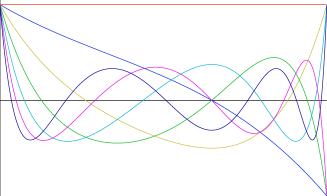
Fig. 4: $\mathcal{P}_{3n}(x),\hskip 3.0ptn=0-6$.

For ${\nu}=3$ polynomial composition (13) results in sequence

$$\mathcal{P}_{30}(x)=1,$$

$$\mathcal{P}_{31}(x)=-2x^{3}+2x^{2}-2x+1,$$

$$\mathcal{P}_{32}(x)=6x^{6}-12x^{5}+18x^{4}-18x^{3}+12x^{2}-6x+1,$$

$$\mathcal{P}_{33}(x)=-20x^{9}+60x^{8}-120x^{7}+170x^{6}-180x^{5}+150x^{4}-92x^{3}+42x^{2}-12x+1,$$

$$\mathcal{P}_{34}=(x)=70x^{12}-280x^{11}+700x^{10}-1260x^{9}+1750x^{8}-1960x^{7}+1770x^{6}$$

$$-1300x^{5}+760x^{4}-340x^{3}+110x^{2}-20x+1,$$

$$\mathcal{P}_{35}(x)=252x^{15}-1260x^{14}+3780x^{13}-8190x^{12}+13860x^{11}-19152x^{10}+21980x^{9}$$

$$-21210x^{8}+17220x^{7}-11690x^{6}+6552x^{5}-2940x^{4}+1010x^{3}-240x^{2}+30x+1,$$

$$\mathcal{P}_{36}(x)=924x^{18}-5544x^{17}+19404x^{16}-48972x^{15}+97020x^{14}-158004x^{13}+216594x^{12}$$

$$-253764x^{11}+256032x^{10}-223020x^{9}+167454x^{8}-107604x^{7}+58464x^{6}$$

$$-26292x^{5}+9450x^{4}-2562x^{3}+462x^{2}-42x+1.$$

From properties of Legendre polynomials it follows that $\mathcal{P}_{\nu n}(x)$ with $\nu=3$ and any odd $n$ have a zero at $x=0.647798871...$ . Calculations show that an increase in $\nu$ leads to an increase in this value of $x$ in the interval $[0,1]$, and the zeros cluster towards $x=1$.

Polynomials $\mathcal{P}_{{\nu}n}(x)$ have $n$ real zeros and $(\nu-1)n$ complex conjugate zeros. We find that transmutation (12) results in redistribution of real zeros of the standard orthogonal polynomials and parameter $\nu$ can be selected to increase density of the zeros near $x=1$.

Transmuted orthogonal polynomials are bases in $L_{2}[0,1]$. The polynomials originate compositions that are similar to those introduced in sections 2 - 5, 8 - 10.

References

- [1] J.P. Boyd, Orthogonal rational functions on a semi-infinite interval, J. Comput. Phys., Vol. 70, No 1, (1987), pp. 63-88.
- [2] A. Bultheel, P. Gonźales Vera, E. Hendriksen, O. Njåstad, Orthogonal rational functions, Cambridge Monographs on Applied and Computational Mathematics, Vol. 5, Cambridge University Press, Cambridge, 1999.
- [3] A. Cayley, Sur quelques propriétés des déterinants gauches, Journal fr die reine und undewandte Mathematik, 32: pp. 119-123, 1846.
- [4] V. S. Chelyshkov, Sequences of exponential polynomials orthogonal on the semi-axis, Dokl. Akad. Nauk Ukr. SSR, Ser. A, No 1, pp. 14 –17, 1987.
- [5] V. S. Chelyshkov, Alternative orthogonal polynomials and quadratures, Electron. Trans. Numer. Anal., Vol. 25, pp. 17-26, 2006.
- [6] V. S. Chelyshkov, Alternative Jacobi polynomials and orthogonal exponentials, arXiv:1105.1838, 11pp., 2011.
- [7] V. Chelyshkov, Alternative orthogonal rational functions on a half line, arXiv:1504.05248, 8 pp., 2015.
- [8] V. S. Chelyshkov, Spectral shape preserving approximation, arXiv:1801.09282, 15pp., 2020.
- [9] Seng Cheng, Jie Shen, Log orthogonal functions: approximation properties and applications, arXiv:2003.01209, 24 pp., 2020.
- [10] Guo, Ben-Yu; Shen, Jie; Wang, Zhong-Qing, Chebyshev rational spectral and pseudospectral methods on a semi-infinite interval, Int. J. Numer. Methods Eng. 53 (1), pp. 65–84, 2002.
- [11] O. Jaroch, Approximation by exponential functions, Aplikace Matematiky, Vol. 7, No 4, pp. 249 – 264, 1962 (in Czech).
- [12] T.N. Koorwinder, R. Wong, R. Koekoek, R.F. Swarttouw, Orthogonal polynomials, in NIST Handbook of Mathematical Functions. Cambridge University Press, 2010. (dlmf.nist.gov).
- [13] A.-M. Legendre, Recherches sur l’attraction des sphéroides homogènes, Mémoires de Mathématiques. et de Physique, préséntes à ĺAcadémie Royale des Sciences, par divers savans, et las dans ses Assemblées. Vol. X. Paris, pp. 411-435, 1785 (1782).
- [14] J. Van Deun, A. Bultheel, Orthogonal rational functions and quadrature on an interval, Journal of computational and applied mathematics, 153: pp. 487-495, 2003.
- [15] Wang Zhong-Qing, Guo Ben-Yu, A mixed spectral method for incompressible fluid flow in an infinite strip, Journal of Computational and Applied Mathematics, Volume 24, N.3, pp. 343-364, 2005.