capbtabboxtable[][]

Appendix of GLIPv2: Unifying Localization and Vision-Language Understanding

The appendix is organized as follows:

• In Section  1, we provide more visualizations of our model’s predictions on various localization and VL understanding tasks.

• In Section  2, we describe all our evaluated tasks and their dataset in detail.

• In Section  3, we introduce the training details and hyperparameters used in Section 4 in the main paper.

• In Section  4, we provide a more detailed analysis for the ablation of adding pre-training losses (refer to Section 4 in the main paper).

• In Section  5, we provide more results for all the checkpoints of adding pre-training data (refer to Section 4 in the main paper).

• In Section  6, we provide a detailed analysis of the experiments of grounded captioning (mentioned in Section 4 in the main paper).

• In Section  7, we give out a comparison for the model’s inference speed.

• In Section  8, we present per-dataset results for all experiments in ODinW.

Figure 1: GLIPv2, a pre-trained grounded VL understanding model, unifies various localization and VL understanding tasks. These two kinds of tasks mutually benefit each other, and enables new capabilities such as language-guided detection/segmentation and grounded VQA/captioning.

1 Visualization

We provide a clearer illustration of GLIPv2 in Figure  1, which elegantly unifies various localization (object detection, instance segmentation) and VL understanding (phrase grounding, VQA and captioning) tasks. More visualizations of the predictions under various tasks from GLIPv2 are also provided to indicate the model’s strength and capability. Please refer to Figure  2 for OD / Grounding, Figure  3 for Instance / Referring Image Segmentation, and Figure  4 for Grounded VL Understanding.

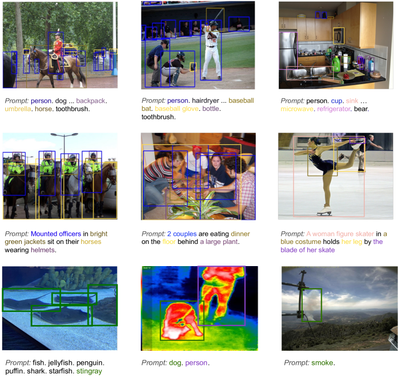
Figure 2: Visualization for OD / Grounding. Row 1: Object Detection on COCO. Row 2: Phrase Grounding on Flickr30K. Row 3: Object Detection on ODinW.

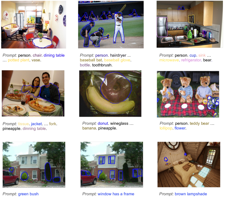
Figure 3: Visualization for Instance / Referring Image Segmentation. Row 1: Instance Segmentation on COCO Mask. Row 2: Instance Segmentation on LVIS. Row 3: Referring Image Segmentation on PhraseCut.

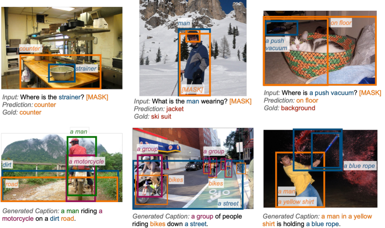
Figure 4: Visualization for Grounded VL Understanding. Row 1: Grounded VQA predictions (The model is given the input question and a placeholder token “[MASK]” for the answer. The model can ground not only entities in the question, but also the implied answer entity). Row 2: Grounded captioning on COCO (The model can generate high-quality captions and at the meantime, provide localization results.

2 Tasks and dataset descriptions

2.1 (Language-guided) object detection and phrase grounding

COCO. caesar2018coco The Microsoft Common Objects in Context dataset is a medium-scale object detection dataset. It has about 900k bounding box annotations for 80 object categories, with about 7.3 annotations per image. It is one of the most used object detection datasets, and its images are often used within other datasets (including VG and LVIS).

ODinW. We use 13 datasets from Roboflow. Roboflow hosts over 30 datasets, and we exclude datasets that are too challenging (e.g., detecting different kinds of chess pieces) or impossible to solve without specific domain knowledge (e.g., understanding sign language). We provide the details of the 13 datasets we use in Table 1. We include the PASCAL VOC 2012 dataset as a reference dataset, as public baselines have been established on this dataset. For PascalVOC, we follow the convention and report on the validation set. For Pistols, there are no official validation or test sets so we split the dataset ourselves.

Table 1: 13 ODinW dataset statistics. We summarize the objects of interest for each dataset and report the image number of each split.

Dataset	Objects of Interest	Train/Val/Test	URL
PascalVOC	Common objects (PascalVOC 2012)	13690/3422/-	https://public.roboflow.com/object-detection/pascal-voc-2012
AerialDrone	Boats, cars, etc. from drone images	52/15/7	https://public.roboflow.com/object-detection/aerial-maritime
Aquarium	Penguins, starfish, etc. in an aquarium	448/127/63	https://public.roboflow.com/object-detection/aquarium
Rabbits	Cottontail rabbits	1980/19/10	https://public.roboflow.com/object-detection/cottontail-rabbits-video-dataset
EgoHands	Hands in ego-centric images	3840/480/480	https://public.roboflow.com/object-detection/hands
Mushrooms	Two kinds of mushrooms	41/5/5	https://public.roboflow.com/object-detection/na-mushrooms
Packages	Delivery packages	19/4/3	https://public.roboflow.com/object-detection/packages-dataset
Raccoon	Raccoon	150/29/17	https://public.roboflow.com/object-detection/raccoon
Shellfish	Shrimp, lobster, and crab	406/116/58	https://public.roboflow.com/object-detection/shellfish-openimages
Vehicles	Car, bus, motorcycle, truck, and ambulance	878/250/126	https://public.roboflow.com/object-detection/vehicles-openimages
Pistols	Pistol	2377/297/297	https://public.roboflow.com/object-detection/pistols/1
Pothole	Potholes on the road	465/133/67	https://public.roboflow.com/object-detection/pothole
Thermal	Dogs and people in thermal images	142/41/20	https://public.roboflow.com/object-detection/thermal-dogs-and-people

Flickr30k-entities. plummer2015flickr30k Given one more phrases, which may be inter-related, the phrase grounding task is to provide a set of bounding boxes for each given phrase. We use the Flickr30k-entities dataset for this task, with the train/val/test splits as provided by li2021grounded and evaluate our performance in terms of Recall. Flickr30K is included in the gold grounding data so we directly evaluate the models after pre-training as in MDETR kamath2021mdetr. We predict use the any-box-protocol specified in MDETR.

2.2 (Language-guided) instance segmentation and referring image segmentation

LVIS. gupta2019lvis The Large Vocabulary Instance Segmentation dataset has over a thousand object categories, following a long-tail distribution with some categories having only a few examples. Similar to VG, LVIS uses the same images as in COCO, re-annotated with more object categories. In contrast to COCO, LVIS is a federated dataset, which means that only a subset of categories is annotated in each image. Annotations therefore include positive and negative object labels for objects that are present and categories that are not present, respectively. In addition, LVIS categories are not pairwise disjoint, such that the same object can belong to several categories.

PhraseCut. wu2020phrasecut Besides object detection, we show that our GLIPv2 can be extended to perform segmentation by evaluating the referring expression segmentation task of the recent PhraseCutwu2020phrasecut which consists of images from VG, annotated with segmentation masks for each referring expression. These expressions comprise a wide vocabulary of objects, attributes and relations, making it a challenging benchmark. Contrary to other referring expression segmentation datasets, in PhraseCut the expression may refer to several objects and the model is expected to find all the corresponding instances.

2.3 VQA and image captioning

VQA. goyal2017making requires the model to predict an answer given an image and a question. We conduct experiment on the VQA2.0 dataset, which is constructed using images from COCO. It contains 83k images for training, 41k for validation, and 81k for test. We treat VQA as a classification problem with an answer set of 3,129 candidates following the common practice of this task. For our best models, we report test-dev and test-std scores by submitting to the official evaluation server.

COCO image captioning. chen2015microsoft The goal of image captioning is to generate a natural language description given an input image. We evaluate GLIPv2 on COCO Captioning dataset and report BLEU-4, CIDEr and SPICE scores on the Karparthy test split.

3 Training details and hyperparamters

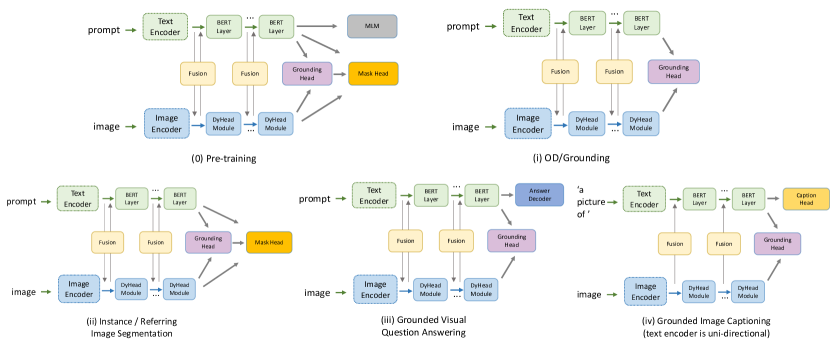
Figure 5: The model architecture for pre-training (0), and downstream tasks (i) OD / Grounding (ii) Instance / Referring Image Segmentation (iii) Grounded Visual Question Answering (iv) Grounded Image Captioning.

3.1 Pre-training

Pre-training data. There are three different types of data in pre-training 1) detection data 2) grounding data 3) caption data, as shown in Table  2. The detection data includes Object365  shao2019objects365, COCO caesar2018coco, OpenImages krasin2017openimages, Visual Genome krishna2017visual, and ImageNetBoxes imagenet. The grounding data includes GoldG, 0.8M human-annotated gold grounding data curated by MDETR kamath2021mdetr combining Flick30K, VG Caption, and GQA hudson2019gqa. The Cap4M is a 4M image-text pairs collected from the web with boxes generated by GLIP-T(C) in li2021grounded, and CC (Conceptual Captions) + SBU (with 1M data).

Model	Image	Text	Pre-Train Data
			Detection	Grounding	Caption
GLIPv2-T	Swin-T	BERT-Base	O365	GoldG (no COCO)	Cap4M
GLIPv2-B	Swin-B	CLIP	O365, COCO, OpenImages, VG, ImageNetBoxes	GoldG	CC15M+ SBU
GLIPv2-H	CoSwin-H yuan2021florence	CLIP	O365, COCO, OpenImages, VG, ImageNetBoxes	GoldG	CC15M+SBU
Mask Head	–	–	LVIS, COCO	PhraseCut	–

Table 2: A detailed list of GLIPv2 model variants

Implementation details. In Section 4 in the main paper, we introduced GLIPv2-T, GLIPv2-B, GLIPv2-H, and we introduce the implementation details in the following.

We pre-train GLIPv2-T based on Swin-Tiny models with 32 GPUs and a batch size of 64. We use a base learning rate of $1\times 10^{-5}$ for the language backbone (BERT-Base) and $1\times 10^{-4}$ for all other parameters. The learning rate is stepped down by a factor of 0.1 at the 67% and 89% of the total 330,000 training steps. We decay the learning rate when the zero-shot performance on COCO saturates. The max input length is 256 tokens for all models. To optimize the results for object detection, we continue pre-training without the MLM loss for another 300,000 steps.

We pre-train GLIPv2-B based on Swin-Base models with 64 GPUs and a batch size of 64. We use a base learning rate of $1\times 10^{-4}$ for all parameters, including the language backbone (CLIP-type pre-layernorm transformer). The learning rate is stepped down by a factor of 0.1 at the 67% and 89% of the total 1 million training steps. We decay the learning rate when the zero-shot performance on COCO saturates. The max input length is 256 tokens for all models. To optimize the results for object detection, we continue pre-training without the MLM loss for another 500,000 steps.

We pre-train GLIPv2-H based on the CoSwin-Huge model from Florence yuan2021florence with 64 GPUs and a batch size of 64. We use a base learning rate of $1\times 10^{-4}$ for all parameters, including the language backbone (CLIP-type pre-layernorm transformer). The learning rate is stepped down by a factor of 0.1 at the 67% and 89% of the total 1 million training steps. We decay the learning rate when the zero-shot performance on COCO saturates. The max input length is 256 tokens for all models. We found that there is no need to continue pre-training without MLM loss for the huge model.

Mask heads of GLIPv2-T, GLIPv2-B and GLIPv2-H are pre-trained COCO, LVIS and PhraseCut, while freezing all the other model parameters. This mask head pre-training uses batch size 64, and goes through COCO for 24 epochs, LVIS for 24 epochs, and PhraseCut for 8 epochs, respectively. GLIPv2 uses Hourglass network newell2016stacked as instance segmentation head feature extractor, and utilizes the "classification-to-matching" trick to change the instance segmentation head linear prediction layer (outputs $K$-dimensional logits on each pixel) to a dot product layer between pixel visual features and the word features after VL fusion. GLIPv2-T and GLIPv2-B use a very basic Hourglass network for segmentation head feature extractor: only 1 scale and 1 layer, with hidden dimension 256. GLIPv2-H uses a larger Hourglass network for segmentation head feature extractor: 2 scales and 4 layers, with hidden dimension 384.

3.2 Downstream tasks

OD / Grounding. When fine-tuning on COCO, we use a base learning rate of $1\times 10^{-5}$ and 24 training epochs for the pre-trained GLIPv2-T model, and a base learning rate of $5\times 10^{-6}$ and 5 training epochs for the pre-trained GLIPv2-B and GLIPv2-H models.

For direct evaluation on LVIS, since LVIS has over 1,200 categories and they cannot be fit into one text prompt, so we segment them into multiple chunks, fitting 40 categories into one prompt and query the model multiple times with the different prompts. We find that models tend to overfit on LVIS during the course of pre-training so we closely monitor the performance on minival for all models and report the results with the best checkpoints in Table 2 in the main paper.

For direct evaluation on Flickr30K, models may also overfit during the course of pre-training so we monitor the performance on the validation set for all models and report the results with the best checkpoints in Table 2 in the main paper.

Instance segmentation / Referring Image Segmentation. Given the pre-trained model with pre-trained mask head, we simply fine-tune the entire network to get the task-specific fine-tuned models.

For fine-tuning on COCO instance segmentation, we use a base learning rate of $1\times 10^{-5}$ and 24 training epochs for the pre-trained GLIPv2-T model, and a base learning rate of $5\times 10^{-6}$ and 5 training epochs for the pre-trained GLIPv2-B and GLIPv2-H models.

For fine-tuning on LVIS instance segmentation, we use a base learning rate of $1\times 10^{-5}$ and 24 training epochs for the pre-trained GLIPv2-T model, and a base learning rate of $5\times 10^{-6}$ and 5 training epochs for the pre-trained GLIPv2-B and GLIPv2-H models.

For fine-tuning on PhraseCut Referring Image segmentation, we use a base learning rate of $1\times 10^{-5}$ and 12 training epochs for the pre-trained GLIPv2-T model, and a base learning rate of $5\times 10^{-6}$ and 3 training epochs for the pre-trained GLIPv2-B and GLIPv2-H models.

(Grounded) VQA. To fine-tune GLIPv2 for VQA, we feed the image and question into the model and then take the output feature sequence $P$ from the language side (after the VL fusion) and apply a ‘attention pooling’ layer to obtain a feature vector $P_{vqa}$. More specifically, the attention pooling layer applies a linear layer followed by softmax to obtain normalized scaler weights, and then these weights are used to compute a weighted sum to produce the feature vector $p_{vqa}$. This feature vector is then fed to a 2-layer MLP with GeLU activation hendrycks2016gaussian and a final linear layer to obtain the logits for the 3129-way classification. Following standard practice teney2018tips, we use binary cross entropy loss to take account of different answers from multiple human annotators. Following VinVL Zhang_2021_CVPR, we train on the combination of train2014 + val2014 splits of the VQAv2 dataset, except for the reserved 2k dev split.. For the ablation studies we report the accuracy on this 2k dev split.

Other than the conventional VQA setting, we also experimented a new ‘grounded VQA’ setup, which the model is required to not only predict the answer, but also ground the objects (predict bounding boxes in the image) mentioned in the question and answer text, see Figure  5(iii). Note that the language input is the question appended by a [MASK] token, and this [MASK] token should ground to the object if the answer is indeed an object in the image. The total training loss is summing the grounding loss (intra-image region-word contrastive loss) and the VQA loss described previously.

(Grounded) Image Captioning. We fine-tune the pre-trained model on COCO Caption “Karpathy” training split. The training objective is uni-directional Language Modeling (LM), which maximizes the likelihood of the next word at each position given the image and the text sequence before it. To enable autoregressive generation, we use uni-directional attention mask for the text part, and prevent the image part from attending to the text part in the fusion layers. Although the training objective (LM) is different from that in pre-training (i.e., bi-directional MLM), we directly fine-tune the model for image captioning to evaluate its capability of generalizing to VL generation tasks. Our model is trained with cross entropy loss only, without using CIDEr optimization.

For grounded image captioning (Figure  5), we add the grounding loss (intra-image region-word contrastive loss) in training, which is calculated in the same way as in pre-training. We use Flickr30K training split for this task. During inference, for each predicted text token, we get its dot product logits with all the region representations and choose the maximum as the associated bounding box.

4 More analysis on pre-training loss

Table 4 in the main paper shows the performance of the downstream tasks with different variants of our method. Compared to the GLIP pre-training tasks with only intra-image region-word contrastive loss (Row 3), adding inter-image word-region loss (Row 5) substantially improves the pre-trained model performance across all the object detection tasks (COCO, ODinW, and LVIS) on both zero-shot and fine-tuned manner. Consistent with common observations from most VL understanding methods, adding MLM loss (row4) benefits for learning the representation for understanding tasks (Flick30k, VQA, and Captioning). Furthermore, using all three losses together at the 1st stage pre-training and doing the 2nd stage pre-training without MLM on OD and GoldG data, GLIPv2 (Row6) can perform well on both the localization and VL understanding tasks.

5 More analysis on pre-training data

Table 5 in the main paper reports the last checkpoint results on GLIPv2 when we do the scaling up of pre-training data. As more weak image-text pair data (Cap) is involved in our training, it benefits both standard/in-domain (i.e., COCO, Flickr30K) and large-domain gap (i.e., ODinW, LVIS) tasks. We also show that by adding the inter-image region-word contrastive helps when we are fixing the data at the same scale. For large-domain gap tasks, adding the inter-image region-word contrastive loss will further boost the model to learn better representation. For more detailed scaling-up effects on various tasks under all the checkpoints for GLIP and GLIPv2, see Figure  6.

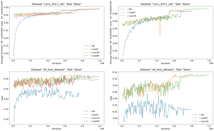
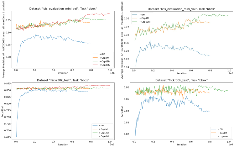
Figure 6: Pre-train data scale up on Base-scale model. Left: GLIP, Right: GLIPv2; Row 1: COCO minival, Row 2: ODinW test split, Row 3: LVIS minival, Row 4: Flick30K test.

6 Experiments on grounded image captioning

The grounded captioning task requires the model to generate an image caption and also ground predicted phrases to object regions. The final predictions consist of (1) the text captions (2) predicted object regions, and (3) the grounding correspondence between the phrases and regions. Following the established benchmarks ma2020learning; zhou2020unified, we evaluate the caption metrics on COCO Captions and report the grounding metrics on Flick30K, as shown in Table  3.

Model	COCO Caption			Flickr30K Grounding
	B@4	CIDEr	SPICE	R@1	R@5	R@10
No Pretrain	35.4	115.3	21.2	77.0	92.9	95.7
+ $L_{\text{mlm}}$	33.4	107.6	19.9	70.9	90.0	93.2
+ $L_{\text{loc}}+L_{\text{intra}}+L_{\text{inter}}$	36.6	120.3	21.6	80.8	94.9	96.7
GLIPv2-T	36.5	119.8	21.6	80.8	94.4	96.5
GLIPv2-B	37.4	123.0	21.9	81.0	94.5	96.5

Table 3: Grounded image captioning results on the COCO Caption, and Flickr30K Entities. We report BLEU@4, CIDer, and SPICE metrics for caption evaluation, and we use R@1, R@5, R@10 for grounding evaluation.

7 Inference speed

We test the inference speed for GLIPv2 on V100 with batch size 1 and show its comparison to MDETR, as shown in Table  4.

Table 4: Model inference speed on various tasks. We report FPS, which is the number of images processed per second per GPU (higher is better).

Model	Object Detection (COCO)	Phrase Grounding (Flick30K)	Referring Expression Segmentation (PhraseCut)
MDETR R101  kamath2021mdetr	–	9.31	3.80
MDETR EffB3  kamath2021mdetr	–	11.20	3.98
MDETR EffB5  kamath2021mdetr	–	9.15	–
GLIPv2-T	4.12	3.74	2.26
GLIPv2-B	3.01	3.23	2.39
GLIPv2-H	1.21	1.13	0.89

8 All results for ODinW

We report the per-dataset performance under 0,1,3,5,10-shot and full data as well as linear probing, prompt tuning, and full-model tuning in Table  5 and Table  6 (on the next pages).

Table 5: Zero-shot performance on 13 ODinW datasets.

Model	PascalVOC	AerialDrone	Aquarium	Rabbits	EgoHands	Mushrooms	Packages	Raccoon	Shellfish	Vehicles	Pistols	Pothole	Thermal	Avg
GLIP-T	56.2	12.5	18.4	70.2	50.0	73.8	72.3	57.8	26.3	56.0	49.6	17.7	44.1	46.5
GLIP-L	61.7	7.1	26.9	75.0	45.5	49.0	62.8	63.3	68.9	57.3	68.6	25.7	66.0	52.1
GLIPv2-T	57.6	10.5	18.4	71.4	52.7	77.7	67.7	58.8	27.8	55.6	60.1	20.0	52.4	48.5
GLIPv2-B	62.8	8.6	18.9	73.7	50.3	83.0	68.6	61.6	56.0	53.8	67.8	32.6	53.8	54.2
GLIPv2-H	66.3	10.9	30.4	74.6	55.1	52.1	71.3	63.8	66.2	57.2	66.4	33.8	73.3	55.5

Table 6: Per-dataset performance of DyHead, GLIP-T, GLIP-L, and GLIPv2-T, GLIPv2-B and GLIPv2-H. For PascalVOC, we report the mAP (IoU=0.50:0.95) using the COCO evaluation script, to be consistent with other 12 datasets. “Prompt” denotes prompt tuning. “Full” denotes full-model tuning.

Model

Shot

Tune

PascalVOC

AerialDrone

Aquarium

Rabbits

EgoHands

Mushrooms

Packages

Raccoon

Shellfish

Vehicles

Pistols

Pothole

Thermal

Avg

DyHead O365

1

Full

25.8$\pm$3.0

16.5$\pm$1.8

15.9$\pm$2.7

55.7$\pm$6.0

44.0$\pm$3.6

66.9$\pm$3.9

54.2$\pm$5.7

50.7$\pm$7.7

14.1$\pm$3.6

33.0$\pm$11.0

11.0$\pm$6.5

8.2$\pm$4.1

43.2$\pm$10.0

33.8$\pm$3.5

DyHead O365

3

Full

40.4$\pm$1.0

20.5$\pm$4.0

26.5$\pm$1.3

57.9$\pm$2.0

53.9$\pm$2.5

76.5$\pm$2.3

62.6$\pm$13.3

52.5$\pm$5.0

22.4$\pm$1.7

47.4$\pm$2.0

30.1$\pm$6.9

19.7$\pm$1.5

57.0$\pm$2.3

43.6$\pm$1.0

DyHead O365

5

Full

43.5$\pm$1.0

25.3$\pm$1.8

35.8$\pm$0.5

63.0$\pm$1.0

56.2$\pm$3.9

76.8$\pm$5.9

62.5$\pm$8.7

46.6$\pm$3.1

28.8$\pm$2.2

51.2$\pm$2.2

38.7$\pm$4.1

21.0$\pm$1.4

53.4$\pm$5.2

46.4$\pm$1.1

DyHead O365

10

Full

46.6$\pm$0.3

29.0$\pm$2.8

41.7$\pm$1.0

65.2$\pm$2.5

62.5$\pm$0.8

85.4$\pm$2.2

67.9$\pm$4.5

47.9$\pm$2.2

28.6$\pm$5.0

53.8$\pm$1.0

39.2$\pm$4.9

27.9$\pm$2.3

64.1$\pm$2.6

50.8$\pm$1.3

DyHead O365

All

Full

53.3

28.4

49.5

73.5

77.9

84.0

69.2

56.2

43.6

59.2

68.9

53.7

73.7

60.8

GLIP-T

1

Prompt

54.4$\pm$0.9

15.2$\pm$1.4

32.5$\pm$1.0

68.0$\pm$3.2

60.0$\pm$0.7

75.8$\pm$1.2

72.3$\pm$0.0

54.5$\pm$3.9

24.1$\pm$3.0

59.2$\pm$0.9

57.4$\pm$0.6

18.9$\pm$1.8

56.9$\pm$2.7

49.9$\pm$0.6

GLIP-T

3

Prompt

56.8$\pm$0.8

18.9$\pm$3.6

37.6$\pm$1.6

72.4$\pm$0.5

62.8$\pm$1.3

85.4$\pm$2.8

64.5$\pm$4.6

69.1$\pm$1.8

22.0$\pm$0.9

62.7$\pm$1.1

56.1$\pm$0.6

25.9$\pm$0.7

63.8$\pm$4.8

53.7$\pm$1.3

GLIP-T

5

Prompt

58.5$\pm$0.5

18.2$\pm$0.1

41.0$\pm$1.2

71.8$\pm$2.4

65.7$\pm$0.7

87.5$\pm$2.2

72.3$\pm$0.0

60.6$\pm$2.2

31.4$\pm$4.2

61.0$\pm$1.8

54.4$\pm$0.6

32.6$\pm$1.4

66.3$\pm$2.8

55.5$\pm$0.5

GLIP-T

10

Prompt

59.7$\pm$0.7

19.8$\pm$1.6

44.8$\pm$0.9

72.1$\pm$2.0

65.9$\pm$0.6

87.4$\pm$1.1

72.3$\pm$0.0

57.5$\pm$1.2

30.0$\pm$1.4

62.1$\pm$1.4

57.8$\pm$0.9

33.5$\pm$0.1

73.1$\pm$1.4

56.6$\pm$0.2

GLIP-T

All

Prompt

66.4

27.6

50.9

70.6

73.3

88.1

67.7

64.0

40.3

65.4

68.3

50.7

78.5

62.4

GLIP-T

1

Full

54.8$\pm$2.0

18.4$\pm$1.0

33.8$\pm$1.1

70.1$\pm$2.9

64.2$\pm$1.8

83.7$\pm$3.0

70.8$\pm$2.1

56.2$\pm$1.8

22.9$\pm$0.2

56.6$\pm$0.5

59.9$\pm$0.4

18.9$\pm$1.3

54.5$\pm$2.7

51.1$\pm$0.1

GLIP-T

3

Full

58.1$\pm$0.5

22.9$\pm$1.3

40.8$\pm$0.9

65.7$\pm$1.6

66.0$\pm$0.2

84.7$\pm$0.5

65.7$\pm$2.8

62.6$\pm$1.4

27.2$\pm$2.7

61.9$\pm$1.8

60.7$\pm$0.2

27.1$\pm$1.2

70.4$\pm$2.5

54.9$\pm$0.2

GLIP-T

5

Full

59.5$\pm$0.4

23.8$\pm$0.9

43.6$\pm$1.4

68.7$\pm$1.3

66.1$\pm$0.6

85.4$\pm$0.4

72.3$\pm$0.0

62.1$\pm$2.0

27.3$\pm$1.2

61.0$\pm$1.8

62.7$\pm$1.6

34.5$\pm$0.5

66.6$\pm$2.3

56.4$\pm$0.4

GLIP-T

10

Full

59.1$\pm$1.3

26.3$\pm$1.1

46.3$\pm$1.6

67.3$\pm$1.5

67.1$\pm$0.7

87.8$\pm$0.5

72.3$\pm$0.0

57.7$\pm$1.7

34.6$\pm$1.7

65.4$\pm$1.4

61.6$\pm$1.0

39.3$\pm$1.0

74.7$\pm$2.3

58.4$\pm$0.2

GLIP-T

All

Full

62.3

31.2

52.5

70.8

78.7

88.1

75.6

61.4

51.4

65.3

71.2

58.7

76.7

64.9

GLIP-L

1

Prompt

62.8$\pm$0.4

18.0$\pm$1.8

37.4$\pm$0.3

71.9$\pm$2.4

68.9$\pm$0.1

81.8$\pm$3.4

65.0$\pm$2.8

63.9$\pm$0.4

70.2$\pm$1.2

67.0$\pm$0.4

69.3$\pm$0.1

27.6$\pm$0.4

69.8$\pm$0.6

59.5$\pm$0.4

GLIP-L

3

Prompt

65.0$\pm$0.5

21.4$\pm$1.0

43.6$\pm$1.1

72.9$\pm$0.7

70.4$\pm$0.1

91.4$\pm$0.7

57.7$\pm$3.7

70.7$\pm$1.1

69.7$\pm$0.9

62.6$\pm$0.8

67.7$\pm$0.4

36.2$\pm$1.1

68.8$\pm$1.5

61.4$\pm$0.3

GLIP-L

5

Prompt

65.6$\pm$0.3

19.9$\pm$1.6

47.7$\pm$0.7

73.7$\pm$0.7

70.6$\pm$0.3

86.8$\pm$0.5

64.6$\pm$0.7

69.4$\pm$3.3

68.0$\pm$1.3

67.8$\pm$1.5

68.3$\pm$0.3

36.6$\pm$1.6

71.9$\pm$0.6

62.4$\pm$0.5

GLIP-L

10

Prompt

65.9$\pm$0.2

23.4$\pm$2.6

50.3$\pm$0.7

73.6$\pm$0.7

71.8$\pm$0.3

86.5$\pm$0.3

70.5$\pm$1.1

69.0$\pm$0.5

69.4$\pm$2.4

70.8$\pm$1.2

68.8$\pm$0.6

39.3$\pm$0.9

74.9$\pm$2.1

64.2$\pm$0.4

GLIP-L

All

Prompt

72.9

23.0

51.8

72.0

75.8

88.1

75.2

69.5

73.6

72.1

73.7

53.5

81.4

67.9$\pm$0.0

GLIP-L

1

Full

64.8$\pm$0.6

18.7$\pm$0.6

39.5$\pm$1.2

70.0$\pm$1.5

70.5$\pm$0.2

69.8$\pm$18.0

70.6$\pm$4.0

68.4$\pm$1.2

71.0$\pm$1.3

65.4$\pm$1.1

68.1$\pm$0.2

28.9$\pm$2.9

72.9$\pm$4.7

59.9$\pm$1.4

GLIP-L

3

Full

65.6$\pm$0.6

22.3$\pm$1.1

45.2$\pm$0.4

72.3$\pm$1.4

70.4$\pm$0.4

81.6$\pm$13.3

71.8$\pm$0.3

65.3$\pm$1.6

67.6$\pm$1.0

66.7$\pm$0.9

68.1$\pm$0.3

37.0$\pm$1.9

73.1$\pm$3.3

62.1$\pm$0.7

GLIP-L

5

Full

66.6$\pm$0.4

26.4$\pm$2.5

49.5$\pm$1.1

70.7$\pm$0.2

71.9$\pm$0.2

88.1$\pm$0.0

71.1$\pm$0.6

68.8$\pm$1.2

68.5$\pm$1.7

70.0$\pm$0.9

68.3$\pm$0.5

39.9$\pm$1.4

75.2$\pm$2.7

64.2$\pm$0.3

GLIP-L

10

Full

66.4$\pm$0.7

32.0$\pm$1.4

52.3$\pm$1.1

70.6$\pm$0.7

72.4$\pm$0.3

88.1$\pm$0.0

67.1$\pm$3.6

64.7$\pm$3.1

69.4$\pm$1.4

71.5$\pm$0.8

68.4$\pm$0.7

44.3$\pm$0.6

76.3$\pm$1.1

64.9$\pm$0.7

GLIP-L

All

Full

69.6

32.6

56.6

76.4

79.4

88.1

67.1

69.4

65.8

71.6

75.7

60.3

83.1

68.9

GLIPv2-T

1

Prompt

51.2$\pm$0.3

17.7$\pm$1.2

34.2$\pm$0.1

68.7$\pm$1.2

67.3$\pm$0.9

83.7$\pm$2.1

68.1$\pm$1.7

53.4$\pm$0.2

30.0$\pm$0.9

59.0$\pm$0.1

60.0$\pm$0.3

21.9$\pm$0.2

66.5$\pm$0.7

52.4$\pm$0.5

GLIPv2-T

3

Prompt

66.6$\pm$0.2

11.5$\pm$0.7

37.2$\pm$1.0

71.7$\pm$0.3

70.1$\pm$0.4

45.7$\pm$0.1

57.7$\pm$1.2

69.7$\pm$1.5

42.7$\pm$0.4

67.5$\pm$0.9

65.6$\pm$1.0

36.7$\pm$1.2

69.2$\pm$1.2

55.6$\pm$0.4

GLIPv2-T

5

Prompt

58.9$\pm$1.2

17.4$\pm$0.6

42.8$\pm$0.4

72.6$\pm$0.5

66.1$\pm$0.2

84.9$\pm$0.8

69.7$\pm$0.6

65.5$\pm$2.1

35.6$\pm$0.8

62.8$\pm$0.9

59.8$\pm$0.2

35.5$\pm$0.9

74.4$\pm$0.2

57.4$\pm$0.4

GLIPv2-T

10

Prompt

59.9$\pm$0.4

21.6$\pm$2.0

43.7$\pm$0.3

74.3$\pm$0.4

68.2$\pm$0.7

88.1$\pm$0.1

72.0$\pm$0.9

60.0$\pm$0.4

35.6$\pm$1.2

66.1$\pm$0.6

61.0$\pm$0.3

42.8$\pm$0.4

70.9$\pm$3.2

58.8$\pm$0.5

GLIPv2-T

All

Prompt

67.4

22.3

50.5

74.3

73.4

85.5

74.7

65.8

53.7

67.4

68.9

52.3

83.7

64.8$\pm$0.0

GLIPv2-T

1

Full

64.8$\pm$0.6

18.7$\pm$0.6

39.5$\pm$1.2

70.0$\pm$1.5

70.5$\pm$0.2

69.8$\pm$18.0

70.6$\pm$4.0

68.4$\pm$1.2

71.0$\pm$1.3

65.4$\pm$1.1

68.1$\pm$0.2

28.9$\pm$2.9

72.9$\pm$4.7

52.8$\pm$1.4

GLIPv2-T

3

Full

53.9$\pm$0.1

17.8$\pm$0.7

42.7$\pm$1.1

73.1$\pm$1.0

65.9$\pm$0.2

84.7$\pm$3.4

69.7$\pm$0.8

60.7$\pm$1.3

28.8$\pm$0.8

61.7$\pm$1.3

60.6$\pm$0.2

35.5$\pm$0.4

68.3$\pm$1.7

55.6$\pm$0.7

GLIPv2-T

5

Full

58.9$\pm$0.2

17.4$\pm$1.1

42.8$\pm$1.3

72.6$\pm$0.7

66.1$\pm$0.6

84.9$\pm$0.9

69.7$\pm$0.3

65.5$\pm$1.0

35.6$\pm$0.9

62.8$\pm$0.3

59.8$\pm$0.2

35.5$\pm$1.2

74.4$\pm$2.1

57.4$\pm$0.4

GLIPv2-T

10

Full

57.6$\pm$1.0

27.6$\pm$1.2

49.1$\pm$1.0

70.4$\pm$0.5

69.2$\pm$0.2

88.1$\pm$0.0

73.1$\pm$2.3

58.0$\pm$2.8

42.9$\pm$1.2

64.8$\pm$0.2

62.1$\pm$0.9

39.9$\pm$0.4

71.6$\pm$0.8

59.7$\pm$0.3

GLIPv2-T

All

Full

66.4

30.2

52.5

74.8

80.0

88.1

74.3

63.7

54.4

63.0

73.0

60.1

83.5

66.5

GLIPv2-B

1

Prompt

68.7$\pm$0.1

19.9$\pm$0.3

38.4$\pm$0.8

68.5$\pm$1.0

68.6$\pm$0.8

87.7$\pm$3.0

69.3$\pm$1.7

68.5$\pm$0.4

55.2$\pm$0.3

65.7$\pm$0.7

67.2$\pm$0.1

34.8$\pm$0.8

69.6$\pm$0.4

60.4$\pm$0.3

GLIPv2-B

3

Prompt

67.2$\pm$0.6

22.2$\pm$0.3

46.5$\pm$0.9

71.2$\pm$0.8

70.9$\pm$0.1

86.9$\pm$0.2

67.7$\pm$1.8

63.7$\pm$2.3

46.9$\pm$0.8

68.1$\pm$0.4

67.4$\pm$0.9

47.9$\pm$1.0

78.9$\pm$1.7

62.0$\pm$0.5

GLIPv2-B

5

Prompt

68.9$\pm$1.0

25.7$\pm$0.4

50.5$\pm$0.9

73.8$\pm$1.5

69.7$\pm$0.6

84.9$\pm$0.3

69.3$\pm$0.7

65.8$\pm$1.6

65.7$\pm$1.0

69.2$\pm$0.3

67.5$\pm$0.7

34.0$\pm$0.2

73.1$\pm$0.6

62.9$\pm$0.4

GLIPv2-B

10

Prompt

69.4$\pm$0.7

21.8$\pm$1.3

48.7$\pm$0.2

71.3$\pm$0.2

71.0$\pm$0.7

88.1$\pm$0.4

68.6$\pm$0.7

73.5$\pm$0.3

61.5$\pm$1.9

69.3$\pm$0.2

68.6$\pm$0.7

41.3$\pm$0.2

75.2$\pm$1.3

63.8$\pm$0.3

GLIPv2-B

All

Prompt

71.9

26.1

50.6

74.5

73.5

86.9

74.9

71.0

71.6

71.0

72.4

50.2

80.5

67.3$\pm$0.0

GLIPv2-B

1

Full

67.8$\pm$0.4

18.7$\pm$0.3

44.2$\pm$0.9

71.4$\pm$0.3

70.4$\pm$1.2

87.9$\pm$7.3

66.1$\pm$2.4

68.9$\pm$1.1

60.6$\pm$1.6

68.1$\pm$0.6

69.0$\pm$0.7

35.1$\pm$0.9

68.9$\pm$2.1

61.2$\pm$0.6

GLIPv2-B

3

Full

68.1$\pm$0.2

25.7$\pm$0.4

46.4$\pm$1.6

69.8$\pm$1.3

71.3$\pm$1.2

88.0$\pm$3.4

68.6$\pm$0.9

69.8$\pm$1.7

60.1$\pm$0.3

68.4$\pm$1.9

68.5$\pm$0.6

39.8$\pm$0.8

71.4$\pm$2.1

62.8$\pm$0.8

GLIPv2-B

5

Full

68.6$\pm$1.0

21.6$\pm$0.6

46.7$\pm$0.7

70.9$\pm$0.9

71.0$\pm$1.2

88.1$\pm$3.7

69.1$\pm$0.2

71.8$\pm$1.0

61.5$\pm$0.7

68.7$\pm$0.2

69.3$\pm$0.8

40.2$\pm$1.0

74.8$\pm$2.8

63.3$\pm$0.6

GLIPv2-B

10

Full

67.4$\pm$1.3

22.3$\pm$1.1

50.5$\pm$0.7

74.3$\pm$0.4

73.4$\pm$0.4

85.5$\pm$0.1

74.7$\pm$0.9

65.8$\pm$2.4

53.7$\pm$1.1

67.4$\pm$0.9

68.9$\pm$0.7

52.3$\pm$0.6

83.7$\pm$3.2

64.6$\pm$0.3

GLIPv2-B

All

Full

71.1

32.6

57.5

73.6

80.0

88.1

74.9

68.2

70.6

71.2

76.5

58.7

79.6

69.4

GLIPv2-H

1

Prompt

68.3$\pm$0.6

16.4$\pm$0.6

45.8$\pm$0.3

72.0$\pm$0.5

67.9$\pm$0.9

89.3$\pm$3.2

69.3$\pm$1.7

67.9$\pm$0.8

66.3$\pm$1.9

68.0$\pm$0.7

66.8$\pm$0.3

33.9$\pm$0.4

70.7$\pm$1.5

61.4$\pm$0.5

GLIPv2-H

3

Prompt

69.5$\pm$0.7

25.9$\pm$0.2

50.0$\pm$1.2

75.4$\pm$1.4

70.1$\pm$0.9

85.9$\pm$2.5

69.3$\pm$0.7

70.8$\pm$1.2

66.4$\pm$0.8

68.0$\pm$1.2

68.8$\pm$0.9

34.0$\pm$0.3

72.7$\pm$1.6

63.6$\pm$0.6

GLIPv2-H

5

Prompt

69.4$\pm$0.7

22.0$\pm$0.6

49.1$\pm$0.1

70.7$\pm$1.0

73.0$\pm$0.5

88.1$\pm$0.8

70.3$\pm$0.4

71.2$\pm$1.8

62.9$\pm$1.4

70.1$\pm$0.3

68.3$\pm$0.6

42.7$\pm$0.6

74.3$\pm$0.5

63.9$\pm$0.7

GLIPv2-H

10

Prompt

66.0$\pm$0.7

27.5$\pm$1.3

53.8$\pm$0.2

74.6$\pm$0.2

80.1$\pm$0.7

87.4$\pm$0.4

69.3$\pm$0.7

66.0$\pm$0.3

51.2$\pm$1.9

67.2$\pm$0.2

72.8$\pm$0.7

58.3$\pm$0.2

76.5$\pm$1.3

65.5$\pm$0.6

GLIPv2-H

All

Prompt

71.2

31.1

57.1

75.0

79.8

88.1

68.6

68.3

59.6

70.9

73.6

61.4

78.6

69.1$\pm$0.0

GLIPv2-H

1

Full

67.8$\pm$0.6

17.3$\pm$0.6

50.7$\pm$0.3

63.8$\pm$0.5

67.3$\pm$0.9

89.4$\pm$3.2

69.3$\pm$1.7

68.2$\pm$0.8

66.6$\pm$1.9

66.8$\pm$0.7

67.0$\pm$0.3

34.0$\pm$0.4

75.0$\pm$1.5

61.7$\pm$0.5

GLIPv2-H

3

Full

62.3$\pm$0.2

29.1$\pm$0.4

53.8$\pm$1.6

72.7$\pm$1.3

78.4$\pm$1.2

85.8$\pm$3.4

68.6$\pm$0.9

60.7$\pm$1.7

43.6$\pm$0.3

65.9$\pm$1.9

72.2$\pm$0.6

55.9$\pm$0.8

81.1$\pm$2.1

64.1$\pm$0.8

GLIPv2-H

5

Full

66.4$\pm$1.0

23.4$\pm$0.6

50.7$\pm$0.7

73.9$\pm$0.9

71.8$\pm$1.2

84.2$\pm$3.7

71.2$\pm$0.2

68.1$\pm$1.0

67.4$\pm$0.7

70.8$\pm$0.2

65.8$\pm$0.8

54.6$\pm$1.0

75.6$\pm$2.8

64.4$\pm$0.6

GLIPv2-H

10

Full

67.3$\pm$1.3

31.6$\pm$1.1

52.4$\pm$0.7

71.3$\pm$0.4

80.0$\pm$0.4

88.1$\pm$0.1

72.9$\pm$0.9

56.9$\pm$2.4

52.2$\pm$1.1

65.4$\pm$0.9

73.9$\pm$0.7

61.0$\pm$0.6

84.0$\pm$3.2

65.9$\pm$0.3

GLIPv2-H

All

Full

74.4

36.3

58.7

77.1

79.3

88.1

74.3

73.1

70.0

72.2

72.5

58.3

81.4

70.4