Thermodynamics and efficiency of sequentially collisional Brownian particles: The role of drivings

Abstract

Brownian particles placed sequentially in contact with distinct thermal reservoirs and subjected to external driving forces are promising candidates for the construction of reliable thermal engines. In this contribution, we address the role of driving forces for enhancing the machine performance. Analytical expressions for thermodynamic quantities such as power output and efficiency are obtained for general driving schemes. A proper choice of these driving schemes substantially increases both power output and efficiency and extends the working regime. Maximizations of power and efficiency, whether with respect to the strength of the force, driving scheme or both have been considered and exemplified for two kind of drivings: a generic power-law and a periodically drivings.

I Introduction

The construction of nanoscale engines has received a great deal of attention and recent technological advances have made feasible the realization of distinct setups such as quantum-dots Esposito et al. (2010a), colloidal particles Rana et al. (2014); Martínez et al. (2016); Albay et al. (2021), single and coupled systems Golubeva and Imparato (2012a); Mamede et al. (2022) acting as working substance and others Jun et al. (2014). In contrast to their macroscopic counterparts, their main features are strongly influenced by fluctuations when operating at the nanoscale, having several features described within the framework of Stochastic Thermodynamics De Groot and Mazur (1962); Seifert (2012); Van den Broeck (2005); Van den Broeck and Esposito (2010); Peliti and Pigolotti (2021).

Recently a novel approach, coined collisional, has been put forward as a candidate for the projection of reliable thermal engines Rosas et al. (2017, 2018); Noa et al. (2020, 2021); Harunari et al. (2021). They consist of sequentially placing the system (a Brownian particle) in contact with distinct thermal reservoirs and subjected to external driving forces during each stage (stroke) of the cycle. Each stage is characterised by the temperature of the connected thermal reservoir and the external driving force. The time needed to switch between the thermal baths at the end of each stage is neglected. Despite its reliability in distinct situations, such as systems interacting only with a small fraction of the environment and those presenting distinct drivings over each member of system Bennett (1982); Maruyama et al. (2009); Sagawa (2014); Parrondo et al. (2015), the engine can operate rather inefficient depending on the way it is projected (temperatures, kind of driving and duration of each stroke). Hence the importance for strategies to enhance its performance Harunari et al. (2021); Noa et al. (2021). Among the distinct approaches, we cite those based on the maximization of power Verley et al. (2014); Schmiedl and Seifert (2007); Esposito et al. (2009); Cleuren et al. (2015); Van den Broeck (2005); Esposito et al. (2010b); Seifert (2011); Izumida and Okuda (2012); Golubeva and Imparato (2012b); Holubec (2014); Bauer et al. (2016), efficiency Proesmans et al. (2015, 2016); Noa et al. (2021), low/finite dissipation Holubec and Ryabov (2015); Johal (2019) or even the assumption of maximization via largest dissipation Purkayastha et al. (2022).

This paper deals with the above points but with a focus on a different direction, namely the optimization of the engine performance by fine-tuning the driving at each stroke. Such idea is illustrated in a collisional Brownian machine, which has been considered as a working substance in several works, as from the theoretical Jones et al. (2015); Albay et al. (2018); Kumar and Bechhoefer (2018); Paneru and Kyu Pak (2020); Li et al. (2019); Mamede et al. (2022) and experimental point of views Martínez et al. (2016); Krishnamurthy et al. (2016); Blickle and Bechinger (2012); Proesmans et al. (2016); Quinto-Su (2014). The collisional description allows to derive general (and exact) expressions for thermodynamic quantities, such as output power and efficiency, irrespective of the kind of driving Noa et al. (2021). In order to exploit the consequences of a distinct driving each stroke and possible optimizations, two representative examples will be considered: periodically and (generic) power-law drivings. The former consists of a simpler and feasible way to drive Brownian particles out of equilibrium Blickle and Bechinger (2012); Proesmans et al. (2016); Barato and Seifert (2016); Proesmans and Horowitz (2019); Holubec and Ryabov (2018) and providing simultaneous maximizations of the engine Mamede et al. (2022). The latter has been considered not only for generalizing the machine performance beyond constant and linear drivings Noa et al. (2020, 2021), but also to exploit the possibility of obtaining a gain by changing its form at each stroke.

This paper is organized as follows: Sec. II presents the model and the main expressions for the thermodynamic quantities. Efficiency and optimisation is discussed in detail for both classes of drivings in Sec. III. Conclusions and perspectives are addressed in Sec. IV.

II Thermodynamics and Main expressions

We focus on the simplest projection of an engine composed of only two strokes and returning to the initial step after one cycle. The time it takes to complete one cycle is set to $\tau$, with each stroke $\in\{1,2\}$ lasting a time $\tau/2$. During stroke $i$ the Brownian particle of mass $m$ is in contact with a thermal bath at temperature $T_{i}$ and subjected to the external force ${\tilde{f}_{i}(t)}$.

In order to introduce thermodynamic forces and fluxes, we start from the expression for the steady entropy production (averaged over a complete period) given by $\overline{\sigma}=\overline{\dot{Q}}_{1}/T_{1}+\overline{\dot{Q}}_{2}/T_{2}$, where $\overline{\dot{Q}}_{1}$ and $\overline{\dot{Q}}_{2}$ are the exchanged heat in each stroke. By resorting to the first law of Thermodynamics $\overline{\dot{Q}}_{1}+\overline{\dot{Q}}_{2}=-(\overline{\dot{W}}_{1}+\overline{\dot{W}}_{2})$ and expressing $T_{1}$ and $T_{2}$ in terms of the mean $T$ and the difference $\Delta T=T_{2}-T_{1}$, $\overline{\sigma}$ can be rewritten in the following (general) form:

$$\overline{\sigma}=\frac{4T^{2}}{4T^{2}-\Delta T^{2}}\left[-\frac{1}{T}\left(\overline{\dot{W}}_{1}+\overline{\dot{W}}_{2}\right)+\left(\overline{\dot{Q}}_{1}-\overline{\dot{Q}}_{2}\right)\frac{\Delta T}{2T^{2}}\right].$$ (1)

Expressions for work and heat are obtained by considering the time evolution of the system probability distribution $P_{i}(v,t)$, governed by the following Fokker-Planck (FP) equation Tomé and De Oliveira (2015); Tomé and de Oliveira (2010); Van den Broeck and Esposito (2010)

$$\frac{\partial P_{i}}{\partial t}=-\frac{\partial J_{i}}{\partial v}-{\tilde{f}}_{i}(t)\frac{\partial P_{i}}{\partial v}.$$ (2)

Here $J_{i}$ denotes the probability current given by

$$\quad J_{i}=-\gamma_{i}vP_{i}-\frac{\gamma_{i}k_{\textrm{B}}T_{i}}{m}\frac{\partial P_{i}}{\partial v},$$ (3)

with $\gamma_{i}$ the viscous coefficient per mass. Applying the usual boundary conditions in the space of velocities, in which both $P_{i}(v,t)$ and $J_{i}(v,t)$ vanish as $|v|\rightarrow\infty$, the time evolution of system energy $U_{i}(t)=m\langle v_{i}^{2}\rangle/2$ during each stroke corresponds to the sum of two terms:

$$\frac{d}{dt}U_{i}(t)=-[\dot{W}_{i}(t)+\dot{Q}_{i}(t)]$$ (4)

with the mean power $\dot{W}_{i}(t)$ and heat $\dot{Q}_{i}(t)$ given by

$$\dot{W}_{i}(t) = -m\langle v_{i}\rangle(t){\tilde{f}}_{i}(t);$$ (5)

$$\dot{Q}_{i}(t) = \gamma_{i}\left(m\expectationvalue{v_{i}^{2}}(t)-k_{\text{B}}T_{i}\right).$$ (6)

By averaging over a complete period, one recovers the first law of Thermodynamics as stated previously. Similarly, the time evolution of the system entropy $S_{i}(t)=-k_{\mbox{\tiny B}}\langle\ln P_{i}\rangle$ during stage $i$ can be expressed as a difference between two terms:

$$\frac{d}{dt}S_{i}=\sigma_{i}(t)-\Phi_{i}(t),$$ (7)

where $\sigma_{i}(t)$ and $\Phi_{i}(t)$ are the entropy production rate and the entropy flux, respectively, whose expressions are given by

$$\sigma_{i}(t)=\frac{m}{\gamma_{i}T_{i}}\int\frac{J_{i}^{2}}{P_{i}}dv,\qquad{\rm and}\qquad\Phi_{i}(t)=\frac{\dot{Q}_{i}(t)}{T_{i}}.$$ (8)

Note that the right side of Eq. (8) integrated over a complete period is equivalent with the relation for $\overline{\dot{\sigma}}$ given by Eq. (1). Expressions for above thermodynamic quantities in terms of system parameters are obtained by recalling that such class of systems evolve to a nonequilibrium steady state whose probability distribution $P_{i}(v,t)$ for the $i-$th stage, satisfying Eq. (2), is Gaussian,

$$P_{i}(v,t)=\exp{-(v-\langle v_{i}\rangle(t))^{2}/2b_{i}(t)}/\sqrt{2\pi b_{i}(t)}$$ (9)

in which the mean $\langle v_{i}\rangle(t)$ and variance $b_{i}(t)=\langle v_{i}^{2}\rangle(t)-\langle v_{i}\rangle^{2}(t)$ are time dependent and determined by the following equations

$$\frac{d\langle v_{i}\rangle(t)}{dt}=-\gamma_{i}\langle v_{i}\rangle(t)+{\tilde{f}}_{i}(t),$$ (10)

and

$$\frac{db_{i}(t)}{dt}=-2\gamma_{i}b_{i}(t)+\frac{2\gamma_{i}k_{\textrm{B}}T_{i}}{m},$$ (11)

respectively. In order to obtain explicit and general results, external forces are expressed in the following form:

$${\tilde{f}}_{i}(t)=\begin{cases}X_{1}g_{1}(t),\quad t\in[0,\tau/2]\\ X_{2}g_{2}(t),\quad t\in[\tau/2,\tau],\end{cases}$$ (12)

where $g_{i}(t)$ and $X_{i}$ account for the kind of driving and its strength at stage $i$, respectively. Continuity of $P_{i}(v,t)$ at times $t=\tau/2$ and $t=\tau$ implies

$$\langle v_{1}\rangle(\tau/2)=\langle v_{2}\rangle(\tau/2)\;\;\;\; ;\;\;\;\;b_{1}(\tau/2)=b_{2}(\tau/2)$$ (13)

$$\langle v_{1}\rangle(0)=\langle v_{2}\rangle(\tau)\;\;\;\; ;\;\;\;\;b_{1}(0)=b_{2}(\tau)$$ (14)

From the above, we arrive at the following general expressions (evaluated for $k_{\mbox{\tiny B}}=1$ and equal $\gamma_{i}=\gamma$):

$$\langle v_{1}\rangle(t) = X_{1}\int_{0}^{t}e^{\gamma(t^{\prime}-t)}g_{1}(t^{\prime})dt^{\prime}+\frac{1}{e^{\gamma\tau}-1}\left\{X_{1}\int_{0}^{\tau/2}e^{\gamma(t^{\prime}-t)}g_{1}(t^{\prime})dt^{\prime}+X_{2}\int_{\tau/2}^{\tau}e^{\gamma(t^{\prime}-t)}g_{2}(t^{\prime})dt^{\prime}\right\},$$ (15)

$$\langle v_{2}\rangle(t) = X_{2}\int_{\tau/2}^{t}e^{\gamma(t^{\prime}-t)}g_{2}(t^{\prime})dt^{\prime}+\frac{1}{e^{\gamma\tau}-1}\left\{e^{\gamma\tau}X_{1}\int_{0}^{\tau/2}e^{\gamma(t^{\prime}-t)}g_{1}(t^{\prime})dt^{\prime}+X_{2}\int_{\tau/2}^{\tau}e^{\gamma(t^{\prime}-t)}g_{2}(t^{\prime})dt^{\prime}\right\},$$ (16)

$$b_{1}(t) = -\frac{1}{m}\frac{(T_{1}-T_{2})}{\left(1+e^{-\gamma\tau}\right)}e^{-2\gamma t}+\frac{T_{1}}{m}\;\;\;\;\;\;\;;\;\;\;\;\;\;\;b_{2}(t)=-\frac{1}{m}\frac{(T_{2}-T_{1})}{\left(1+e^{-\gamma\tau}\right)}e^{-2\gamma(t-\tau/2)}+\frac{T_{2}}{m}.$$ (17)

Inserting the above expressions into Eqs. (5-6) and averaging over a complete cycle we finally arrive at

$$\overline{\dot{W}}_{1} = -\frac{m}{\tau\left(e^{\gamma\tau}-1\right)}\left[X_{1}^{2}\left(\left(e^{\gamma\tau}-1\right)\int_{0}^{\tau/2}g_{1}(t)e^{-\gamma t}\,\int_{0}^{t}g_{1}(t^{\prime})e^{\gamma t^{\prime}}\,dt^{\prime}dt+\int_{0}^{\tau/2}g_{1}(t)e^{-\gamma t}\,dt\int_{0}^{\tau/2}g_{1}(t^{\prime})e^{\gamma t^{\prime}}\,dt^{\prime}\right)\right.$$ (18)

$$+ X_{1}X_{2}\left.\int_{0}^{\tau/2}g_{1}(t)e^{-\gamma t}\,dt\int_{\tau/2}^{\tau}g_{2}(t^{\prime})e^{\gamma t^{\prime}}\,dt^{\prime}\right],$$

$${\overline{\dot{Q}}_{1}} = \frac{\gamma m}{\tau}\left[\int_{0}^{\tau/2}\langle v_{1}\rangle^{2}dt-\frac{1}{2\gamma m}\tanh(\gamma\tau/2)(T_{1}-T_{2})\right],$$ (19)

and

$$\overline{\dot{W}}_{2} =-\frac{m}{\tau(e^{\gamma\tau}-1)}\bigg{[}X_{2}^{2}\bigg{(}\int_{\tau/2}^{\tau}g_{2}(t)e^{-\gamma t}dt\int_{\tau/2}^{\tau}g_{2}(t^{\prime})e^{\gamma t^{\prime}}dt^{\prime}+(e^{\gamma\tau}-1)\int_{\tau/2}^{\tau}g_{2}(t)e^{-\gamma t}\int_{\tau/2}^{t}g_{2}(t^{\prime})e^{\gamma t^{\prime}}dt^{\prime}dt\bigg{)}.$$

$$+X_{1}X_{2}\bigg{(}\int_{\tau/2}^{\tau}g_{2}(t)e^{-\gamma t}\,dt\int_{0}^{\tau/2}g_{1}(t^{\prime})e^{\gamma t^{\prime}}\,dt^{\prime}+(e^{\gamma\tau}-1)\int_{\tau/2}^{\tau}e^{-\gamma}g_{2}(t)dt\int_{0}^{\tau/2}e^{\gamma t^{\prime}}g_{1}(t)dt^{\prime}\bigg{)}\bigg{]},$$ (20)

$${\overline{\dot{Q}}_{2}} =\frac{m\gamma}{\tau}\bigg{[}\int_{\tau/2}^{\tau}\langle v_{2}\rangle^{2}dt+\frac{1}{2\gamma m}\tanh(\gamma\tau/2)(T_{1}-T_{2})\bigg{]},$$ (21)

for first and second stages, respectively and $\overline{\sigma}$ is promptly obtained by inserting above expressions in Eq. (1). It is worth emphasizing that Eqs. (18)-(21) are general and valid for any kind of drivings and temperatures. Close to equilibrium the entropy production (Eq. (1)) assumes the familiar flux times force form $\overline{\sigma}\approx J_{1}f_{1}+J_{2}f_{2}+J_{T}f_{T}$ with forces

$$f_{1}=X_{1}/T\;\;;\;\;f_{2}=X_{2}/T\;\;;\;\;f_{T}=\Delta T/T^{2}\;$$ (22)

($\Delta T=T_{2}-T_{1}$) and fluxes defined by

$$\overline{\dot{W}}_{1}=-TJ_{1}f_{1}\;\;;\;\;\overline{\dot{W}}_{2}=-TJ_{2}f_{2}\;\;;\;\;\overline{\dot{Q}}_{1}-\overline{\dot{Q}}_{2}=2J_{T}.$$ (23)

Up to first order in the forces these fluxes can be expressed in terms of Onsager coefficients $J_{1}=L_{11}f_{1}+L_{12}f_{2}$, $J_{2}=L_{21}f_{1}+L_{22}f_{2}$ and $J_{T}=L_{TT}f_{T}$ which results in

$$L_{11} = \frac{mT}{\tau\left(e^{\gamma\tau}-1\right)}\left[\left(e^{\gamma\tau}-1\right)\int_{0}^{\tau/2}g_{1}(t)e^{-\gamma t}\int_{0}^{t}g_{1}(t^{\prime})e^{\gamma t^{\prime}}\,dt^{\prime}dt\,+\int_{0}^{\tau/2}g_{1}(t)e^{-\gamma t}dt\,\int_{0}^{\tau/2}g_{1}(t^{\prime})e^{\gamma t^{\prime}}\,dt^{\prime}\right],$$ (24)

$$L_{22} = \frac{mT}{\tau\left(e^{\gamma\tau}-1\right)}\left[\int_{\tau/2}^{\tau}g_{2}(t)e^{-\gamma t}\,dt\int_{\tau/2}^{\tau}g_{2}(t^{\prime})e^{\gamma t^{\prime}}\,dt^{\prime}+\left(e^{\gamma\tau}-1\right)\int_{\tau/2}^{\tau}g_{2}(t)e^{-\gamma t}\int_{\tau/2}^{t}g_{2}(t^{\prime})e^{\gamma t^{\prime}}\,dt^{\prime}dt\,\right],$$ (25)

$$L_{12} = \frac{mT}{\tau\left(e^{\gamma\tau}-1\right)}\int_{0}^{\tau/2}g_{1}(t)e^{-\gamma t}\,dt\int_{\tau/2}^{\tau}g_{2}(t^{\prime})e^{\gamma t^{\prime}}\,dt^{\prime}\;\;\;\;\;\;;\;\;\;\;\;\;L_{21}=\frac{mTe^{\gamma\tau}}{\tau\left(e^{\gamma\tau}-1\right)}\int_{0}^{\tau/2}g_{1}(t^{\prime})e^{\gamma t^{\prime}}\,dt^{\prime}\int_{\tau/2}^{\tau}g_{2}(t)e^{-\gamma t}\,dt,$$ (26)

$$L_{TT} = \dfrac{T^{2}}{2\tau}\tanh{\left(\dfrac{\gamma\tau}{2}\right)}.$$ (27)

Two remarks are in order. First, to verify Onsager-Casimir symmetry for the cross coefficients $L_{12}$ and $L_{21}$ it is necessary not only to reverse the drivings but also to exchange the indices $1\leftrightarrow 2$ as argued in Rosas et al. (2018). Second, there is no coupling between work fluxes and heat flux. That is, the cross coefficients $L_{T1}$, $L_{1T}$, $L_{T2}$ and $L_{2T}$ are absent. Hence this class of engines does not convert heat into work (and vice versa) and always loses its efficiency when the difference of temperatures $\Delta T$ between thermal baths is large, because heat can not be converted into output work Noa et al. (2021); Mamede et al. (2022).

As we gonna to see next, for the regime of temperatures we shall concern, efficiency properties can be solely expressed in terms of Onsager coefficients and their derivatives.

III Efficiency

As stated before, our aim is to adjust the drivings in order to optimize the system performance. More concretely, given an amount of energy injected to the system, whether in the form of input work $\overline{\dot{W}}_{\text{in}}\equiv\overline{\dot{W}}_{\text{1}}<0$ and/or heat $\overline{\dot{Q}}_{\text{in}}=\overline{\dot{Q}}_{1}\Theta(-\overline{\dot{Q}}_{1})+\overline{\dot{Q}}_{2}\Theta(-\overline{\dot{Q}}_{2})<0$ ($\Theta(x)$ denoting the Heaviside function), it is partially converted into power output ${\cal P}\equiv\overline{\dot{W}}_{\text{2}}\geq 0$. A measure of such conversion is characterized by the efficiency, given as the ratio between above quantities:

$$\eta=-\frac{{\cal P}}{{\overline{\dot{W}_{\rm in}}}+{\overline{\dot{Q}_{\rm in}}}}.$$ (28)

In order to obtain a first insight about the role driving, we shall split the analysis in two parts: engine operating at an unique temperature but the driving is changed each half stage. Next, we extend for different temperatures and distinct drivings.

III.1 Overview about Brownian work-to-work converters and distinct maximizations routes

Work-to-work converters have been studied broadly in the context of biological motors such as kinesin Liepelt and Lipowsky (2007, 2009) and myosin, in which chemical energy is converted into mechanical and vice-versa Hooyberghs et al. (2013). More recently, distinct work-to-work converters made of Brownian engines have been attracted considerable attention and in this section we briefly revise their main aspects Proesmans et al. (2016); Proesmans and Van den Broeck (2017); Noa et al. (2020, 2021); Mamede et al. (2022). Setting $\Delta T=0$ (hence $f_{T}=0$) reduces the efficiency Eq. (28) to the ratio between Onsager coefficients: Noa et al. (2020, 2021); Mamede et al. (2022)

$$\eta\equiv-\frac{{\cal P}}{\overline{\dot{W}}_{\text{in}}}=-\frac{L_{22}f_{2}^{2}+L_{21}f_{1}f_{2}}{L_{12}f_{1}f_{2}+L_{11}f_{1}^{2}}.$$ (29)

For any kind of driving and period, the engine regime ${\cal P}>0$ implies that the absolute value for the output force $f_{2}$ must lie in the interval $0\leq|f_{2}|\leq|f_{m}|$, where $f_{m}=-L_{21}f_{1}/L_{22}$. Since power, efficiency and dissipation are not independent from each other, $f_{m}$ can be related with $f_{2mS}$ (for $f_{1}$ and driving parameter constants), in which the dissipation is minimal. It is straightforward to show that $f_{m}=f_{2mS}+(L_{12}-L_{21})f_{1}/(2L_{22})$. Note that $f_{m}=f_{2mS}$ only when the Onsager coefficients are symmetric, $L_{12}=L_{21}$.

Optimized quantities, whether power and efficiency, can be obtained under three distinct routes: optimization with respect to (i) the output force $f_{2}$ (keeping $f_{1}$ and a driving parameter $\delta$ fixed), (ii) the driving parameter $\delta$ (forces $f_{1}$ and $f_{2}$ held fixed) and (iii) a simultaneous optimization with respect to both $f_{2}$ and $\delta$. As discussed in Refs. Proesmans et al. (2016); Noa et al. (2020, 2021), such optimized quantities can expressed in terms of Onsager coefficients and their derivatives.

The former case (maximization with respect to the output force) is similar to findings from Refs. Proesmans et al. (2016); Noa et al. (2020, 2021), in which the maximum power ${\cal P}_{MP,f_{2}}$ (with efficiency ${\eta}_{MP,f_{2}}$) and maximum efficiency ${\eta}_{ME,f_{2}}$ (with power ${\cal P}_{ME,f_{2}}$) are obtained via optimal adjustments $f_{2MP}$ and $f_{2ME}$. By taking the derivative of ${\cal P}$ and Eq. (29) with respect to $f_{2}$, $f_{2ME}$ and $f_{2MP}$ are given by

$$f_{2ME}=\frac{L_{11}}{L_{12}}\left(-1+\sqrt{1-\frac{L_{12}L_{21}}{L_{11}L_{22}}}\right)f_{1}\quad{\rm and}\quad f_{2MP}=-\frac{1}{2}\frac{L_{21}}{L_{22}}f_{1},$$ (30)

and their associate efficiencies read

$$\eta_{ME,f_{2}}=-\frac{L_{21}}{L_{12}}+\frac{2L_{11}L_{22}}{L_{12}^{2}}\left(1-\sqrt{1-\frac{L_{12}L_{21}}{L_{11}L_{22}}}\right),$$ (31)

and

$$\eta_{MP,f_{2}}=\frac{L_{21}^{2}}{4L_{11}L_{22}-2L_{12}L_{21}},$$ (32)

respectively. Analogous expressions for the power at maximum efficiency ${\cal P}_{ME,f_{2}}$ and the maximum power ${\cal P}_{MP,f_{2}}$ can obtained by inserting $f_{2ME}$ or $f_{2MP}$ into the expression for ${\cal P}$. As stated before, the second maximization to be considered is carried out for fixed output forces and a given driving parameter $\delta$ is adjusted ensuring maximum power $\delta_{MP}$ and/or efficiency $\delta_{ME}$, respectively. According to Ref. Noa et al. (2021); Mamede et al. (2022), they fulfill the following expressions

$$\frac{L^{\prime}_{21}(\delta_{MP})}{L^{\prime}_{22}(\delta_{MP})}=-\frac{f_{2}}{f_{1}},$$ (33)

and

$$\begin{split}\Delta_{2212}(\delta_{ME})&f_{2}^{2}+\Delta_{2111}(\delta_{ME})f_{1}^{2}\\ &+\left[\Delta_{2211}(\delta_{ME})+\Delta_{2112}(\delta_{ME})\right]f_{1}f_{2}=0,\end{split}$$ (34)

respectively, where $L_{ij}^{\prime}(\delta)\equiv\partial L_{ij}(\delta)/\partial\delta$ is the derivative of coefficient $L_{ij}$ respect to the driving $\delta$ and $\Delta_{ijkl}(\delta)=L^{\prime}_{ij}(\delta)L_{kl}(\delta)-L^{\prime}_{kl}(\delta)L_{ij}(\delta)$. Associate maximum power and efficiency are given by

$${\cal P}_{MP,\delta}=\frac{L_{21}^{\prime}(\delta_{MP})}{L_{22}^{\prime 2}(\delta_{MP})}[L_{21}(\delta_{MP})L_{22}^{\prime}(\delta_{MP})-L_{22}(\delta_{MP})L_{21}^{\prime}(\delta_{MP})]f_{1}^{2},$$ (35)

and

$$\eta_{ME,\delta}=-\frac{L_{22}(\delta_{ME})f_{2}^{2}+L_{21}(\delta_{ME})f_{1}f_{2}}{L_{11}(\delta_{ME})f_{1}^{2}+L_{12}(\delta_{ME})f_{1}f_{2}},$$ (36)

respectively, and expressions for ${\cal P}_{ME,\delta}$ and $\eta_{MP,\delta}$ are obtained under a similar way. Although exact and valid for any choice of the drivings $g_{i}(t)$ and forces $f_{i}$, Eqs. (33) and (34), in general, have to be solved numerically for achieving $\delta_{MP}$ and $\delta_{ME}$.

In certain cases (as shall be explained next), it is possible to maximize the engine with respect to the output force $f_{2}$ and a driving parameter $\delta$ simultaneously, which corresponds to the crossing point between maximum lines (power or efficiency) with respect to $f_{2}$ and $\delta$. More specifically, given the loccus of maxima $f_{2MP}/f_{2ME}$ ($\delta$ fixed) and $\delta_{MP}/\delta_{ME}$ ($f_{2}$ fixed), the global $\delta_{MP}^{*}/\delta_{ME}^{*}$ and $f_{2MP}^{*}$/$f_{2ME}^{*}$ corresponds to their intersection. For instance, the global maximization of power is given by Eqs. (30) and (33):

$$\frac{L^{\prime}_{21}(\delta_{MP}^{*})}{L^{\prime}_{22}(\delta_{MP}^{*})}=\frac{1}{2}\frac{L_{21}(\delta_{MP}^{*})}{L_{22}(\delta_{MP}^{*})}\qquad{\rm and}\qquad f_{2MP}^{*}=-\frac{1}{2}\frac{L_{21}(\delta_{MP}^{*})}{L_{22}(\delta_{MP}^{*})}f_{1},$$ (37)

whose (associate global) maximum power ${\cal P}^{*}$ and efficiency $\eta^{*}$read

$${\cal P}^{*}=\frac{1}{4}\frac{L^{2}_{21}(\delta_{MP}^{*})}{L_{22}(\delta_{MP}^{*})}f_{1}^{2},$$ (38)

and

$$\eta^{*}=\frac{L^{2}_{21}(\delta_{MP}^{*})}{4L_{11}(\delta_{MP}^{*})L_{22}(\delta_{MP}^{*})-2L_{21}(\delta_{MP}^{*})L_{12}(\delta_{MP}^{*})},$$ (39)

respectively.

III.2 Applications

Once introduced the main expressions, we are now in position for analyzing the role of driving in our two stage engine. For instance, we shall consider two distinct (but exhibiting complementary features) cases: generically periodically drivings and power-law drivings. As stated before, periodically drivings provided simultaneous maximizations of an autonomous engine Mamede et al. (2022). In this constribution, we adress a simultaneous maximization for our collisional engine. Conversely, power-law drivings has been considered in order to generalize the machine performance beyond constant and linear drivings as well as by exploiting the possibility of improving the engine performance via distinct drivings at each stage Noa et al. (2020, 2021).

III.2.1 Generic periodically driving forces

In this section, we apply the sequential engine under a general periodically driving, having its form and strength in each half stage expressed in terms of its Fourier components:

$$g_{i}(t)=\sum_{n=0}^{\infty}\Big{[}a_{n}^{(i)}\cos(\frac{4\pi n}{\tau}t)+b_{n}^{(i)}\sin(\frac{4\pi n}{\tau}t)\Big{]},$$ (40)

for the $i-$th stage ($i=1$ or $2$), where coefficients $a_{0}^{(i)}$, $a_{n}^{(i)}$ and $b_{n}^{(i)}$ are given by

$$a_{0}^{(i)} =\frac{2}{\tau}\int_{(i-1)\tau/2}^{i\tau/2}g_{i}(t^{\prime})dt^{\prime},$$ (41)

$$a_{n}^{(i)} =\frac{4}{\tau}\int_{(i-1)\tau/2}^{i\tau/2}g_{i}(t^{\prime})\cos(\frac{4\pi n}{\tau}t^{\prime})dt^{\prime},$$ (42)

$$b_{n}^{(i)} =\frac{4}{\tau}\int_{(i-1)\tau/2}^{i\tau/2}g_{i}(t^{\prime})\sin(\frac{4\pi n}{\tau}t^{\prime})dt^{\prime}.$$ (43)

Thermodynamic quantities and maximizations are also exactly obtained from Onsager coefficients, depending on Fourier coefficients $a_{0}^{(i)}$’s, $a_{n}^{(i)}$’s and $b_{n}^{(i)}$’s, whose expressions for generic periodically drivings are listed in Appendix A. In order to tackle the role of the driving under a simpler strategy, from now on, we shall restrict ourselves to the simplest case in which drivings at each stroke present the same frequency, but they differ from phase difference $\phi$ given by

$$g_{1}(t)=\sin(\frac{4\pi}{\tau}t)\;\;\;\;\;;\;\;\;\;\;g_{2}(t)=\sin(\frac{4\pi}{\tau}t-\phi),$$ (44)

The inclusion of a lag $\phi$ in the second half stage has been inspired in recent works in which it can control of power, efficiency Mamede et al. (2022) and dissipation Akasaki et al. (2020) and also by guiding the operation modes of the engine Mamede et al. (2022). Fig. 1 depicts some features for distinct $Tf_{2}$’s and $\phi$’s, respectively.

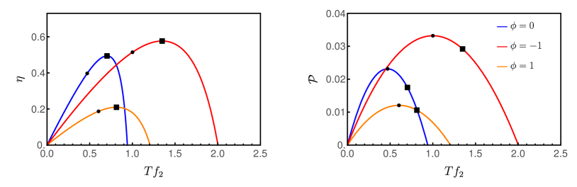
Figure 1: For periodic drivings, the depiction of efficiency $\eta$ and power-output ${\cal P}$ versus force $Tf_{2}$ for distinct $\phi$’s. Squares and circles denote the maximum efficiencies and powers, according to Eq. (31)-(30). In all cases, we set $X_{1}=Tf_{1}=1$, $\tau=2$, $\gamma=k_{B}=m=1$ and $T=1/2$.

First of all, the regime operation is delimited between 0 and $|f_{2m}|$ in which maximization obeys Eqs. (30) (acquiring simpler form given by Eq. [(45)] and a similar expression (although cumbersome) is obtained for $f_{2ME}/f_{1}$. Note that for $\gamma\tau<<1$ and $\gamma\tau>>1$, $f_{2MP}/f_{1}\rightarrow 1/(2\cos\phi)$ and $0$, respectively, such latter being independent on the lag, respectively.

$$\frac{f_{2MP}}{f_{1}}=\frac{4\pi\left(e^{\frac{\gamma\tau}{2}}+1\right)(2\pi\cos(\phi)-\gamma\tau\sin(\phi))}{\gamma\tau\left(\left(e^{\frac{\gamma\tau}{2}}-1\right)\left(\gamma^{2}\tau^{2}+4\pi^{2}\right)-4\gamma\tau\left(e^{\frac{\gamma\tau}{2}}+1\right)\sin^{2}(\phi)\right)+16\pi^{2}\left(e^{\frac{\gamma\tau}{2}}+1\right)\cos^{2}(\phi)},$$ (45)

Fig. 2 reveals additional (and new) features coming from the lag in the second stage. The former is the existence of a two distinct engine regimes for the some values of $Tf_{2}$, being delimited between two intervals $\phi_{1m}\leq\phi\leq\phi_{2m}$ and $\phi_{3m}\leq\phi\leq\phi_{4m}$ (fulfilling ${\cal P}=0$ at $\phi=\phi_{im}$). Also, the change of lag moves the engine regime from positive to negative of $f_{2}$’s. For example, for $\tau=2$ the engine regime yields for positive (negative) output forces for $-\pi/2<\phi\leq\pi/2$ ($\pi/2<\phi\leq\pi$). Finally, in similarity with coupled harmonic chains Mamede et al. (2022), the lag also controls the engine performance, having optimal $\phi_{ME}$ and $\phi_{MP}$ in which $\eta_{ME,\phi}$ and ${\cal P}_{MP,\phi}$, respectively. They obey Eqs. (33)/(46) and (34), the former acquire a simpler expression

$$\frac{f_{2}}{f_{1}}=\frac{\pi[\gamma\tau\csc(\phi_{MP})+2\pi\sec(\phi_{MP})]}{\gamma^{2}\tau^{2}+4\pi^{2}},$$ (46)

for the power and a more cumbersome (not shown) for $\phi_{ME}$. In the limit of $\gamma\tau<<1$ and $\gamma\tau<<1$, Eq. (46) approaches to $\phi_{MP}\rightarrow\cos^{-1}(f_{1}/2f_{2})$ and zero, respectively, such latter independent on the ratio between forces, respectively.

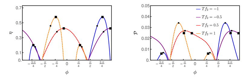
Figure 2: For $\tau=2$ and distinct $Tf_{2}$’s, depiction of efficiency $\eta$ and power-output ${\cal P}$ versus $\phi$. Squares and circles denote the maximum efficiencies and powers, respectively, according to Eqs. (33) and (34). In all cases, we set $X_{1}=Tf_{1}=1$, $\gamma=k_{B}=m=1$ and $T=1/2$.

For completeness, Fig. 3 extends aforementioned efficiency and power findings for other values of $Tf_{2}$ and $\phi$. Note that suitable choices of $\phi$ and $f_{2}$ may lead to a substantial increase of engine performance. For example, for $\phi=0$, the maximum $P_{MP,\delta=0}\approx 0.0231$ and $\eta_{ME,\delta=0}\approx 0.494$, whereas a simultaneous maximization leads to a substantial increase of power-output [given by the intersection between Eqs. (45) and (46)] $P^{*}\approx 0.0398$ and also of $\eta^{*}\approx 0.581$.

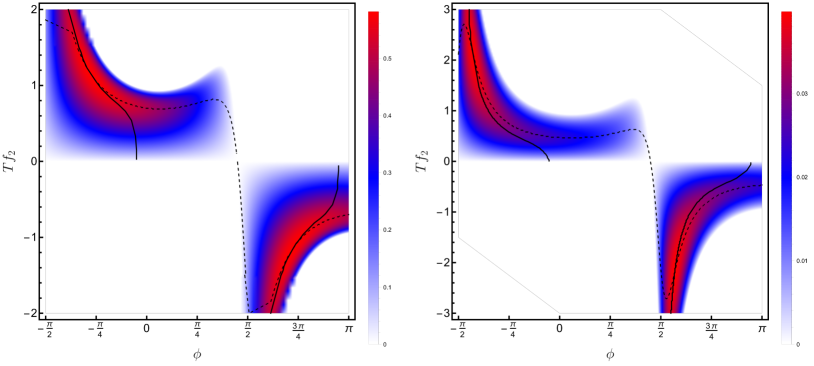
Figure 3: For the set of drivings given by Eq. (44) and $\tau=2$, left and right panels depict the phase diagram of the output force $X_{2}=Tf_{2}$ versus the phase difference $\phi$ for the efficiency and power output, respectively. Continuous and dashed lines denote the maximization with respect to $f_{2}$ and $\phi$, respectively. In all cases, we set $X_{1}=Tf_{1}=1$, $\gamma=k_{B}=m=1$ and $T=1/2$.

III.2.2 Power Law drivings

We consider a general algebraic (power-law) driving acting at each half stage:

$$g(t)=\begin{cases}\big{(}\frac{2t}{\tau}\big{)}^{\alpha},\textrm{ }\textrm{ for }t\in[0,\tau/2]\\ \big{(}1-\frac{2t}{\tau}\big{)}^{\beta},\textrm{ }\textrm{ for }t\in[\tau/2,\tau],\end{cases}$$ (47)

where $\alpha$ and $\beta$ assume non-negative values. It is worth mentioning that particular cases $\alpha=\beta=0$ and $\alpha=\beta=1$ were considered in Ref. Noa et al. (2020). In order to exploit in more details the influence of algebraic drivings into the first (being the worksource and heatsource) and second (responsible for the output work ${\cal P}$) stages, analysis will be carried out by changing each one of them separately [by kepting fixed $\beta$ and $\alpha$ in the former and latter stages, respectively]. Although quantities can be straightforwardly obtained from Eqs. (18)-(26), expressions are very cumbersome (see e.g. appendix B) and for this reason analysis will be restricted for remarkable values of $\alpha$ and $\beta$. In principle, they can assume integer and half-integer values. Nonetheless, inspection of exact expressions reveal that Onsager coefficients assume imaginary values when $\beta$ is half integer. Since half integer values $\alpha$ do not promove substantial changes (not shown), all analysis will be carried out for both $\alpha$ and $\beta$ integers. Thermodynamics quantities are directly obtained from Eqs. (26), whose Onsager coefficients are listed in Appendix B.

Fig. 4 depicts the main portraits of the engine performance by varying the output force for some representative values of $Tf_{2},\alpha$ and $\beta$. Firstly, it reveals that the power output ${\cal P}$ (left panels) is strongly (smoothly) dependent on the shape of driving acting over the first (second) half stage. In the former case, ${\cal P}$ is larger for smaller $\alpha$ [having its maximum for time independent ones ($\alpha=\beta=0$)] and always decreases (for all values of $Tf_{2}$) as $\alpha$ goes up. Unlike the substantial reduction of power output as $\alpha$ is raised, it is $f_{2}$-dependent as $\beta$ (for fixed $\alpha$) is increased, in which ${\cal P}_{mP,f_{2}}$ is mildly decreasing in such case. The increase of $\beta$ confers some remarkable features, such as the substantial increase of range of output forces (e.g. $|f_{2m}|$ increases) in which the system operates as an engine, being restricted to positive (negative) $f_{2}$’s for odd (even) values of $\beta$. Complementary findings are achieved by examining the influence of drivings for the efficiency. Unlike the ${\cal P}$, $\eta$ is $f_{2}$-dependent but $\eta_{mE,f_{2}}$ always increases as $\alpha$ is raised and mildly decreases as $\beta$ goes up. Finally, we stress that $\eta_{mE,f_{2}}$ (squares) and $\eta_{mP,f_{2}}$ (circles) in right panels obey Eqs. (31) and (32), respectively, having their associate ${\cal P}_{ME,f_{2}}$ and ${\cal P}_{MP,f_{2}}$ illustrated in the left panels.

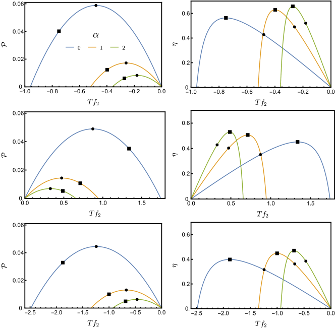
Figure 4: For power-law drivings, the depiction of power output ${\cal P}$ and efficiency $\eta$ versus $X_{2}=Tf_{2}$ for representative values of $\alpha$ and $\beta$ (from top to bottom, $\beta=0,1$ and $2$). Squares and circles denote the maximum efficiencies and powers, according to Eq. (31)-(30). In all cases, we set $X_{1}=Tf_{1}=1$, $\tau=\gamma=k_{B}=m=1$ and $T=1/2$.

Next, we tackle the opposite route, in which $f_{2}$ is kept fixed with $\alpha$ or $\beta$ being varied in order to ensure optimal performance. Maximization of quantities follow theoretical predictions from Eqs. (33) and (34) and Fig. 5 depicts main trends for some representative values of $f_{2}$.

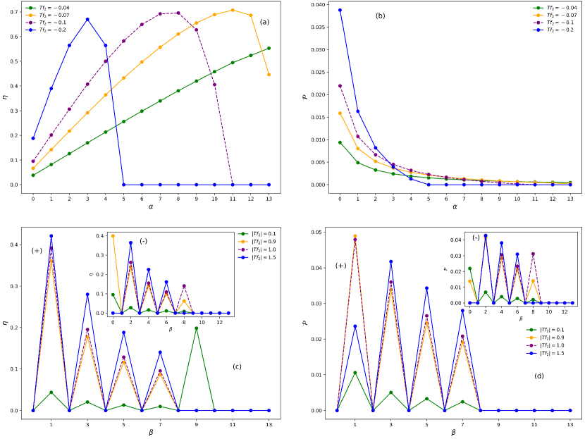
Figure 5: For fixed forces $X_{2}=Tf_{2}$, the depiction of efficiency $\eta$ (a) and ${\cal P}$ (c) versus $\alpha$ ($\beta=0$). Panels (b) and (d) show the same, but $\beta$ is varied (for fixed $\alpha=0$). Main panels (insets) in (c) and (d) show results for odd (even) $\beta$. In all cases, we set $X_{1}=Tf_{1}=1$, $\tau=\gamma=k_{B}=m=1$ and $T=1/2$.

The dependence of driving $\alpha$ upon the efficiency shares some similarities when compared with $f_{2}$ (panel $(a)$), leading to the existence of an optimal driving $\alpha>0$ ($\alpha=0$) for low (large) values of $|f_{2}|$. Hence, a driving beyond the constant case in the first stage can be important for increasing efficiency, depending on the way the machine is projected. On the other hand, for power-output purposes, ${\cal P}_{MP,\alpha=0}$’s are always maxima and decreases for $\alpha>0$, irrespective to the value of output force (panel $(c)$).

The opposite case (fixed $\alpha$ and $\beta$ is varied) is also more revealing and it is $f_{2}$ dependent (see e.g. panels $(c)-(d)$ and Fig. 6), in which maximum efficiencies $\eta_{mE,\beta}$ and powers ${\cal P}_{mP,\beta}$ also follow Eqs. (34) and (33). Fig. 6 extends aforementioned findings for several values of $\alpha$ and $\beta$. In contrast the periodically drivings, a global optimization in such case has not been performed, since $\alpha$ and $\beta$ present only integer values.

Summarizing above findings: While low $\alpha$’s stage is always more advantageous for enhancing the power output, there is a compromise between force $|f_{2}|$ and $\alpha$ and $\beta$ in order to enhance the efficiency. On the other hand, although maximum efficiencies and powers smoothly decreases with $\beta$, the set of output forces $|f_{2}|$ in which the system operates as an engine enlarges substantially.

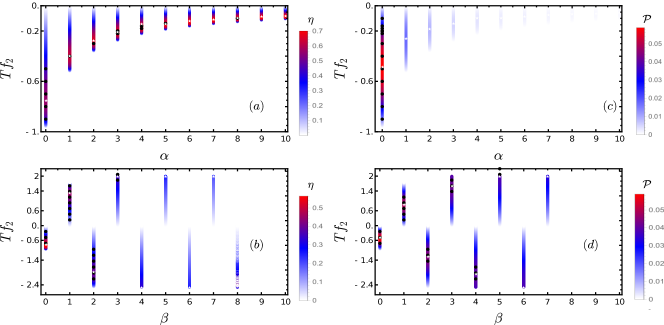
Figure 6: Panels $(a)$ and $(c)$ depict, for $\beta=0$, the phase diagram $X_{2}=Tf_{2}$ versus $\alpha$ by considering the efficiency (a) and power (c). In (b) and (d), the opposite case ($\beta$ is varied for fixed $\alpha=0$). White and black symbols denote some representative maximizations with respect to the $f_{2}$ and driving (for $f_{2}$ held fixed), respectively. In all cases, we set $X_{1}=Tf_{1}=1$, $\tau=\gamma=k_{B}=m=1$ and $T=1/2$.

III.3 Difference of temperatures

In this section we examine the effect of different drivings each stroke when the temperatures are also different. Since ${\cal P}$ does not depend on the temperature, the numerator of Eq. (28) is the same as before, but now the system can receive heat from the thermal bath 1 or 2 if $T_{1}>T_{2}$ or $T_{1}<T_{2}$, respectively and hence such kind of engine becomes less efficiently when the difference of temperatures raises. We wish to investigate the interplay between parameters as a strategy for compensating above point. Taking into account that ${\overline{\dot{Q}}_{1}}$ (or ${\overline{\dot{Q}}_{2}}$) also depends on the $f_{1}$ and $f_{2}$ [appearing inside $\langle v_{1}\rangle(t)$ (or $\langle v_{2}\rangle(t)$)], for small $\Delta T$ the system will receive heat from a thermal bath 1 (2) only if $2m\gamma\int_{0}^{\tau/2}\langle v_{1}\rangle^{2}dt<\tanh(\gamma\tau/2)(T_{1}-T_{2})$ [$2m\gamma\int_{\tau/2}^{\tau}\langle v_{2}\rangle^{2}dt<\tanh(\gamma\tau/2)(T_{2}-T_{1})$]. Otherwise, the thermal engine will behave as a work-to-work converter and all previous analysis and expressions can be applied. For large $\Delta T$ (not considered here), above inequalities are always fulfilled and hence the system efficiency is always lower than the work-to-work case.

Figs. 7 and 8 exemplify thermal engines for periodically drivings. As stated before, although the system operates in a similar way to the work-to-work converter for some values of $Tf_{2}$ (see e.g. symbols $\times$ separating the thermal from work-to-work regimes), the efficiency decreases as $\Delta T$ is raised, illustrating the no conversion of heat into output work. Interestingly, the system placed in contact with the hot thermal bath in the first stage leads to somewhat higher efficiencies ($\eta^{*}\approx 0.547$) than in the first stage $\eta^{*}\approx 0.433$). This can be understood by examining the first term in the right sides of Eqs. (19) and (21). Since the contribution coming from the difference of temperatures is the same in both cases, the interplay between lag and driving forces leads to $\int_{0}^{\tau/2}\langle v_{1}\rangle^{2}(t)dt$ be larger than $\int_{\tau/2}^{\tau}\langle v_{2}\rangle^{2}(t)dt$ and hence confering some advantage when $T_{1}>T_{2}$.

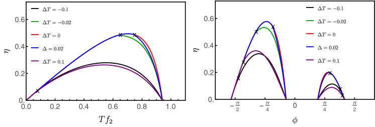
Figure 7: For $\tau=2,\phi=0$ and $Tf_{2}=1$, the depiction of efficiency $\eta$ versus $Tf_{2}$ and $\phi$ for distinct temperature difference $\Delta T$ between thermal baths, respectively. Symbols $\times$ attempt to the separatrix between the work-to-work and thermal engines, respectively. In all cases, we set $T_{1}=1/2$, $T_{2}=1/2+\Delta T$, $X_{1}=Tf_{1}=1$ and $\gamma=k_{B}=m=1$.

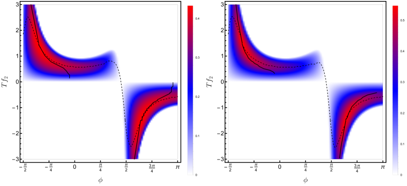
Figure 8: For the set of drivings given by Eq. (44) and $\tau=2$, left and right panels depict efficiency phase diagrams of the output force $X_{2}=Tf_{2}$ versus the phase difference $\phi$ for $\Delta T=0.1$ and $-0.1$, respectively. Continuous and dashed lines denote the maximization with respect to $f_{2}$ and $\phi$, respectively. In all cases, we set $X_{1}=Tf_{1}=1$, $\gamma=k_{B}=m=1$ and $T=1/2$.

Lastly, Fig. 9 extends the results for thermal engines for power-law drivings.

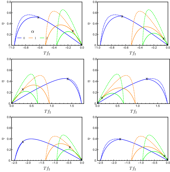
Figure 9: Left and right panels show the efficiency $\eta$ versus $Tf_{2}$ for distinct $\alpha$’s for $\Delta T=0.025$ and $\Delta T=-0.025$, respectively. Symbols $\times$ denote the separatrix between the work-to-work converter (dashed lines) from the heat engine (continuous lines). From top to bottom, $\beta=0,1$ and $2$.

For all values of $\alpha$ and $\beta$, the thermal engine is marked by a reduction of its performance as $\Delta T\neq 0$, being more substantial as $\alpha$ is raised and less sensitive to the increase of driving in the second state (increase of $\beta$). Lastly, the engine performances also exhibit some (small) differences when the hot bath acts over the first and second strokes (see e.g. left and right panels), being somewhat larger when $\Delta T>0$.

IV Conclusions

The influence of the driving in a collisional approach for Brownian engine, in which the particle is subjected each half stage to a distinct force and driving, was investigated from the framework of stochastic Thermodynamics. General and exact expressions for thermodynamic quantities, such as output power and efficiency were obtained, irrespective the kind of driving, period and temperatures. Distinct routes for the maximization of power and efficiency were undertaken, whether with respect to the strength force, driving and both of them for two kind of drivings: generic power-law and periodically drivings. The engine performance can be strongly affected when one considers simple (and different) power law drivings acting over the system at each stage. While a constant driving is always more advantageous for enhancing the power output, a convenient compromise between force $|f_{2}|$, $\alpha$ and $\beta$ can be adopted for improving the efficiency. Conversely, periodically drivings not only allows to perform a simultaneous maximization of engine, in order to obtain a larger gain, but also the change of driving (exemplified by a phase difference in the second stage) confers a second advantage, in which the engine regime is (substantially) enlarged the engine regime over distinct sets of parameters.

As a final comment, it is worth pointing out the decreasing of engine performance as the difference of temperatures between thermal baths is increased. The inclusion of new ingredients, such as a coupling between velocity and drivings, may be a candidate in order to circumvent this fact and be responsible for a better performance of such class of collisional thermal engines.

V Acknowledgments

C.E.F. acknowledges the financial support from São Paulo Research Foundation (FAPESP) under Grants No. 2021/05503-7 and 2021/03372-2. The financial support from CNPq is also acknowledged. This study was supported by the Special Research Fund (BOF) of Hasselt University under grant BOF20BL17.

Appendix A Onsager coefficients for generic periodically driving

Onsager coeficients for a generic periodic driving in each half stage are listed below:

$$L_{11}=\frac{mT}{\tau(e^{\gamma\tau}-1)}\sum_{n=0}^{\infty}\sum_{m=0}^{\infty} \bigg{\{}(e^{\gamma\tau}-1)\int_{0}^{\tau/2}[a_{m}^{(1)}\cos(\frac{4\pi m}{\tau}t)+b_{m}^{(1)}\sin(\frac{4\pi m}{\tau}t)][a_{n}^{(1)}C_{n}^{(1)}(t)+b_{n}^{(1)}S_{n}^{(1)}(t)]e^{-\gamma t}dt+$$

$$+[a_{n}^{(1)}C_{n}^{(1)}(\tau/2)+b_{n}^{(1)}S_{n}^{(1)}(\tau/2)][a_{m}^{(1)}\overline{C}_{m}^{(1)}(\tau/2)+b_{m}^{(1)}\overline{S}_{m}^{(1)}(\tau/2)],\bigg{\}}$$ (48)

$$L_{22}=\frac{mT}{\tau(e^{\gamma\tau}-1)}\sum_{n=0}^{\infty}\sum_{m=0}^{\infty} \bigg{\{}(e^{\gamma\tau}-1)\int_{\tau/2}^{\tau}[a_{m}^{(2)}\cos(\frac{4\pi m}{\tau}t)+b_{m}^{(2)}\sin(\frac{4\pi m}{\tau}t)]\{a_{n}^{(2)}[C_{n}^{(1)}(t)-C_{n}^{(1)}(\tau/2)]+b_{n}^{(2)}[S_{n}^{(1)}(t)-S_{n}^{(1)}(\tau/2)]\}e^{-\gamma t}dt$$

$$+\{a_{n}^{(2)}[C_{n}^{(1)}(\tau)-C_{n}^{(1)}(\tau/2)]+b_{n}^{(2)}[S_{n}^{(1)}(\tau)-S_{n}^{(1)}(\tau/2)]\}\{a_{m}^{(2)}[\overline{C}_{m}^{(1)}(\tau)-\overline{C}_{m}^{(1)}(\tau/2)]+b_{m}^{(2)}[\overline{S}_{m}^{(1)}(\tau)-\overline{S}_{m}^{(1)}(\tau/2)]\}\bigg{\}}$$ (49)

$$L_{12}=\frac{mT}{\tau(e^{\gamma\tau}-1)}\sum_{n=0}^{\infty}\sum_{m=0}^{\infty}\{a_{n}^{(2)}[C_{n}^{(1)}(\tau)-C_{n}^{(1)}(\tau/2)]+b_{n}^{(2)}[S_{n}^{(1)}(\tau)-S_{n}^{(1)}(\tau/2)]\}[a_{m}^{(1)}\overline{C}_{m}^{(1)}(\tau/2)+b_{m}^{(1)}\overline{S}_{m}^{(1)}(\tau/2)]$$ (50)

$$L_{21}=\frac{mTe^{\gamma\tau}}{\tau(e^{\gamma\tau}-1)}\sum_{n=0}^{\infty}\sum_{m=0}^{\infty}[a_{n}^{(1)}C_{n}^{(1)}(\tau/2)+b_{n}^{(1)}S_{n}^{(1)}(\tau/2)]\{a_{m}^{(2)}[\overline{C}_{m}^{(1)}(\tau)-\overline{C}_{m}^{(1)}(\tau/2)]+b_{m}^{(2)}[\overline{S}_{m}^{(1)}(\tau)-\overline{S}_{m}^{(1)}(\tau/2)]\},$$ (51)

where we introduce the following shorthand notation involving quantities $\overline{C}_{m}^{(i)}(t)$, $C_{m}^{(i)}(t)$, $\overline{S}_{m}^{(i)}(t)$ and $S_{m}^{(i)}(t)$

$$C_{n}^{(1)}(t) =\int_{0}^{t}e^{\gamma t^{\prime}}\cos(\frac{4\pi n}{\tau}t^{\prime})dt^{\prime}$$ (52)

$$\overline{C}_{n}^{(1)}(t) =\int_{0}^{t}e^{-\gamma t^{\prime}}\cos(\frac{4\pi n}{\tau}t^{\prime})dt^{\prime}$$ (53)

$$S_{n}^{(1)}(t) =\int_{0}^{t}e^{\gamma t^{\prime}}\sin(\frac{4\pi n}{\tau}t^{\prime})dt^{\prime}$$ (54)

$$\overline{S}_{n}^{(1)}(t) =\int_{0}^{t}e^{-\gamma t^{\prime}}\sin(\frac{4\pi n}{\tau}t^{\prime})dt^{\prime}$$ (55)

For the particular set of drivings from Eq. (44),and considering $\omega_{j}=2\pi/\tau$, Onsager coefficients reduce to the following expressions:

$$L_{11}=\frac{mT\tau\left[\gamma^{3}\tau^{3}+4\pi^{2}\gamma\tau+16\pi^{2}\coth\left(\frac{\gamma\tau}{4}\right)\right]}{4\left(\gamma^{2}\tau^{2}+4\pi^{2}\right)^{2}},$$ (57)

$$L_{22}=\frac{mT\tau\left[\gamma\tau\left(\left(e^{\frac{\gamma\tau}{2}}-1\right)\left(\gamma^{2}\tau^{2}+4\pi^{2}\right)-4\gamma\tau\left(e^{\frac{\gamma\tau}{2}}+1\right)\sin^{2}(\phi)\right)+16\pi^{2}\left(e^{\frac{\gamma\tau}{2}}+1\right)\cos^{2}(\phi)\right]}{4\left(e^{\frac{\gamma\tau}{2}}-1\right)\left(\gamma^{2}\tau^{2}+4\pi^{2}\right)^{2}},$$ (58)

$$L_{12}=-\frac{2\pi mT\tau\coth\left(\frac{\gamma\tau}{4}\right)(\gamma\tau\sin(\phi)+2\pi\cos(\phi))}{\left(\gamma^{2}\tau^{2}+4\pi^{2}\right)^{2}},$$ (59)

and

$$L_{21}=\frac{2\pi mT\tau\coth\left(\frac{\gamma\tau}{4}\right)(\gamma\tau\sin(\phi)-2\pi\cos(\phi))}{\left(\gamma^{2}\tau^{2}+4\pi^{2}\right)^{2}},$$ (60)

respectively.

Appendix B Onsager coefficients for power-law drivings

For generic algebraic (power-law) drivings, Onsager coefficients are listed below:

$$L_{11}=\frac{mT}{\tau}\int_{0}^{\tau/2}\Bigg{[}4^{\alpha}e^{-t}\left(\frac{t}{\tau}\right)^{\alpha}\left(\frac{(-\tau)^{-\alpha}\left(\Gamma\left(\alpha+1,-\frac{\tau}{2}\right)-\Gamma(\alpha+1)\right)}{e^{\tau}-1}+(-t)^{-\alpha}\left(\frac{t}{\tau}\right)^{\alpha}(\Gamma(\alpha+1,-t)-\alpha\Gamma(\alpha))\right)\Bigg{]}dt,$$ (61)

$$L_{12}=\frac{mT}{\tau}\int_{0}^{\tau/2}\Bigg{[}(-1)^{\beta}e^{-t}2^{\alpha+\beta-1}(-\tau)^{-\beta}\text{csch}\left(\frac{\tau}{2}\right)\left(\frac{t}{\tau}\right)^{\alpha}\left(\Gamma\left(\beta+1,-\frac{\tau}{2}\right)-\Gamma(\beta+1)\right)\Bigg{]}dt,$$ (62)

$$L_{21}=\frac{mT}{\tau}\int_{\tau/2}^{\tau}\Bigg{[}\frac{2^{\alpha}(-\tau)^{-\alpha}e^{\tau-t}\left(1-\frac{2t}{\tau}\right)^{\beta}\left(\Gamma\left(\alpha+1,-\frac{\tau}{2}\right)-\Gamma(\alpha+1)\right)}{e^{\tau}-1}\Bigg{]}dt,$$ (63)

and

$$L_{22}=-\frac{mT}{\tau(e^{\tau}-1)}\int_{\tau/2}^{\tau}\Bigg{\{}e^{\frac{\tau}{2}-t}\left(1-\frac{2t}{\tau}\right)^{\beta}\left[\left(\frac{2}{\tau}\right)^{\beta}\left(\Gamma(\beta+1)-\Gamma\left(\beta+1,-\frac{\tau}{2}\right)\right)+\left(e^{\tau}-1\right)\left(2-\frac{4t}{\tau}\right)^{\beta}(\tau-2t)^{-\beta}\left(\Gamma(\beta+1)-\Gamma\left(\beta+1,\frac{\tau}{2}-t\right)\right)\right]\Bigg{\}}dt,$$ (64)

respectively, where $\Gamma(x)$ and $\Gamma(x,y)$ denote gamma and incomplete gamma functions, respectively.

References

- Esposito et al. (2010a) M. Esposito, R. Kawai, K. Lindenberg, and C. Van den Broeck, Phys. Rev. E 81, 041106 (2010a).
- Rana et al. (2014) S. Rana, P. Pal, A. Saha, and A. Jayannavar, Physical review E 90, 042146 (2014).
- Martínez et al. (2016) I. A. Martínez, É. Roldán, L. Dinis, D. Petrov, J. M. Parrondo, and R. A. Rica, Nature physics 12, 67 (2016).
- Albay et al. (2021) J. A. Albay, Z.-Y. Zhou, C.-H. Chang, and Y. Jun, Scientific reports 11, 1 (2021).
- Golubeva and Imparato (2012a) N. Golubeva and A. Imparato, Phys. Rev. Lett. 109, 190602 (2012a).
- Mamede et al. (2022) I. N. Mamede, P. E. Harunari, B. A. N. Akasaki, K. Proesmans, and C. E. Fiore, Phys. Rev. E 105, 024106 (2022).
- Jun et al. (2014) Y. Jun, M. Gavrilov, and J. Bechhoefer, Physical review letters 113, 190601 (2014).
- De Groot and Mazur (1962) S. De Groot and P. Mazur, “North-holland,” (1962).
- Seifert (2012) U. Seifert, Reports on progress in physics 75, 126001 (2012).
- Van den Broeck (2005) C. Van den Broeck, Physical Review Letters 95, 190602 (2005).
- Van den Broeck and Esposito (2010) C. Van den Broeck and M. Esposito, Phys. Rev. E 82, 011144 (2010).
- Peliti and Pigolotti (2021) L. Peliti and S. Pigolotti, Stochastic Thermodynamics: An Introduction (Princeton University Press, 2021).
- Rosas et al. (2017) A. Rosas, C. Van den Broeck, and K. Lindenberg, Phys. Rev. E 96, 052135 (2017).
- Rosas et al. (2018) A. Rosas, C. Van den Broeck, and K. Lindenberg, Phys. Rev. E 97, 062103 (2018).
- Noa et al. (2020) C. F. Noa, W. G. Oropesa, and C. Fiore, Physical Review Research 2, 043016 (2020).
- Noa et al. (2021) C. E. F. Noa, A. L. L. Stable, W. G. C. Oropesa, A. Rosas, and C. E. Fiore, Phys. Rev. Research 3, 043152 (2021).
- Harunari et al. (2021) P. E. Harunari, F. S. Filho, C. E. Fiore, and A. Rosas, Phys. Rev. Research 3, 023194 (2021).
- Bennett (1982) C. H. Bennett, International Journal of Theoretical Physics 21, 905 (1982).
- Maruyama et al. (2009) K. Maruyama, F. Nori, and V. Vedral, Reviews of Modern Physics 81, 1 (2009).
- Sagawa (2014) T. Sagawa, Journal of Statistical Mechanics: Theory and Experiment 2014, P03025 (2014).
- Parrondo et al. (2015) J. M. Parrondo, J. M. Horowitz, and T. Sagawa, Nature physics 11, 131 (2015).
- Verley et al. (2014) G. Verley, M. Esposito, T. Willaert, and C. Van den Broeck, Nature Communications 5, 4721 (2014).
- Schmiedl and Seifert (2007) T. Schmiedl and U. Seifert, EPL (Europhysics Letters) 81, 20003 (2007).
- Esposito et al. (2009) M. Esposito, K. Lindenberg, and C. Van den Broeck, Physical Review Letters 102, 130602 (2009).
- Cleuren et al. (2015) B. Cleuren, B. Rutten, and C. Van den Broeck, The European Physical Journal Special Topics 224, 879 (2015).
- Esposito et al. (2010b) M. Esposito, R. Kawai, K. Lindenberg, and C. Van den Broeck, Physical Review E 81, 041106 (2010b).
- Seifert (2011) U. Seifert, Physical Review Letters 106, 020601 (2011).
- Izumida and Okuda (2012) Y. Izumida and K. Okuda, Europhysics Letters 97, 10004 (2012).
- Golubeva and Imparato (2012b) N. Golubeva and A. Imparato, Physical Review Letters 109, 190602 (2012b).
- Holubec (2014) V. Holubec, Journal of Statistical Mechanics: Theory and Experiment 2014, P05022 (2014).
- Bauer et al. (2016) M. Bauer, K. Brandner, and U. Seifert, Physical Review E 93, 042112 (2016).
- Proesmans et al. (2015) K. Proesmans, C. Driesen, B. Cleuren, and C. Van den Broeck, Physical review E 92, 032105 (2015).
- Proesmans et al. (2016) K. Proesmans, Y. Dreher, M. Gavrilov, J. Bechhoefer, and C. Van den Broeck, Physical Review X 6, 041010 (2016).
- Holubec and Ryabov (2015) V. Holubec and A. Ryabov, Phys. Rev. E 92, 052125 (2015).
- Johal (2019) R. S. Johal, Phys. Rev. E 100, 052101 (2019).
- Purkayastha et al. (2022) A. Purkayastha, G. Guarnieri, S. Campbell, J. Prior, and J. Goold, arXiv preprint arXiv:2202.05264 (2022).
- Jones et al. (2015) P. H. Jones, O. M. Maragò, and G. Volpe, Optical tweezers: Principles and applications (Cambridge University Press, 2015).
- Albay et al. (2018) J. A. Albay, G. Paneru, H. K. Pak, and Y. Jun, Optics express 26, 29906 (2018).
- Kumar and Bechhoefer (2018) A. Kumar and J. Bechhoefer, Applied Physics Letters 113, 183702 (2018).
- Paneru and Kyu Pak (2020) G. Paneru and H. Kyu Pak, Advances in Physics: X 5, 1823880 (2020).
- Li et al. (2019) J. Li, J. M. Horowitz, T. R. Gingrich, and N. Fakhri, Nature communications 10, 1 (2019).
- Krishnamurthy et al. (2016) S. Krishnamurthy, S. Ghosh, D. Chatterji, R. Ganapathy, and A. Sood, Nature Physics 12, 1134 (2016).
- Blickle and Bechinger (2012) V. Blickle and C. Bechinger, Nature Physics 8, 143 (2012).
- Quinto-Su (2014) P. A. Quinto-Su, Nature communications 5, 1 (2014).
- Barato and Seifert (2016) A. C. Barato and U. Seifert, Phys. Rev. X 6, 041053 (2016).
- Proesmans and Horowitz (2019) K. Proesmans and J. M. Horowitz, Journal of Statistical Mechanics: Theory and Experiment 2019, 054005 (2019).
- Holubec and Ryabov (2018) V. Holubec and A. Ryabov, Phys. Rev. Lett. 121, 120601 (2018).
- Tomé and De Oliveira (2015) T. Tomé and M. J. De Oliveira, Stochastic dynamics and irreversibility (Springer, 2015).
- Tomé and de Oliveira (2010) T. Tomé and M. J. de Oliveira, Physical Review E 82, 021120 (2010).
- Liepelt and Lipowsky (2007) S. Liepelt and R. Lipowsky, Phys. Rev. Lett. 98, 258102 (2007).
- Liepelt and Lipowsky (2009) S. Liepelt and R. Lipowsky, Phys. Rev. E 79, 011917 (2009).
- Hooyberghs et al. (2013) H. Hooyberghs, B. Cleuren, A. Salazar, J. O. Indekeu, and C. Van den Broeck, J. Chem. Phys. 139, 134111 (2013).
- Proesmans and Van den Broeck (2017) K. Proesmans and C. Van den Broeck, Chaos: An Interdisciplinary Journal of Nonlinear Science 27, 104601 (2017).
- Akasaki et al. (2020) B. A. Akasaki, M. J. de Oliveira, and C. E. Fiore, Physical Review E 101, 012132 (2020).