Semi-Annihilation of Fermionic Dark Matter

Abstract

The continued non-observation of events emanating from dark matter (DM) annihilations in various direct and indirect detection experiments calls into question the mechanism for determining the relic density of a weakly interacting massive particle. However, if the relic density is determined primarily by a semi-annihilation process, as opposed to the usual annihilation, this tension can be ameliorated. Here, we investigate a $Z_{3}$ symmetric effective field theory incorporating a fermionic dark matter that semi-annihilates to right-handed neutrinos (RHN). The dynamics of the RHN and the impact of its late decays are also scrutinised while obtaining the correct DM relic. Finally, indirect detection bounds on the semi-annihilation cross-sections are drawn from the gamma-ray observations in the direction of Dwarf Spheroidal Galaxies (Fermi-LAT), and including the projections obtained for the H.E.S.S. and the CTA detectors.

1 Introduction

Despite its stupendous success, the Standard Model (SM) leaves many questions unanswered, and, in this article, we aim to address two of them in an unified way. One of these pertains to the existence of Dark Matter (DM) and the other to the problem of neutrino masses. While both the questions have been addressed independently, and, on occasions, even together, we consider a mechanism for establishing the DM relic density that is relatively less explored. Simultaneously, this mechanism would be seen to naturally yield light neutrino masses of the right orders, accommodating equally well both the normal and inverted hierarchy.

A popular mechanism for generating neutrino masses is to invoke the Type-I seesaw mechanism via the introduction of the right-handed neutrinos (RHNs) Minkowski:1977sc ; Mohapatra:1979ia ; Mohapatra:1980yp ; Schechter:1980gr ; Yanagida:1980xy . Being SM gauge singlets, these rarely play any discernible role in laboratory physics other than to generate neutrino masses and mixings and, hence, this sector can hardly be probed, whether directly or indirectly. Attempts have been made to ascribe to these a role in determining the DM relic density, whether through freeze-out or the freeze-in mechanisms Falkowski:2009yz ; Gonzalez-Macias:2016vxy ; Escudero:2016ksa ; Tang:2016sib ; Campos:2017odj ; Batell:2017rol ; Blennow:2019fhy ; Hall:2019rld . In such freeze-out scenarios, the DM particles pair-annihilate primarily to these RHNs which, thereafter, decay to SM particles. Since the RHN has to be lighter than the DM for this to take place, unless the DM itself is very heavy, correct neutrino phenomenology would demand that the neutrino-sector Yukawa couplings be small, thereby delaying the decay of the RHN and, hence, the freeze-out epoch LFZ1 ; LFZ2 ; LFZ3 . Analogous effects are evinced in the freeze-in mechanism as well Bandyopadhyay:2020qpn .

The situation takes an interesting turn if the symmetry ensuring the absolute stability of the DM is not the simple and popular $Z_{2}$. A more complicated symmetry (such as the $Z_{3}$ or $Z_{5}$) may dictate that the the leading interaction is not a pair-annihilation of the DM (whether directly into SM particles or other exotics), but one where, say, three DM particles ${\cal D}$ must be involved Belanger:2012zr ; Choi:2016hid . This could manifest itself in two different ways, a $3{\cal D}\to\sum_{\alpha}{\cal S}_{\alpha}$ annihilation (where ${\cal S}_{\alpha}$ denote $Z_{3}$-neutral particles, whether within the SM or exotic) or of the form ${\cal D}+{\cal D}\to{\cal D}^{*}+\sum_{\alpha}{\cal S}_{\alpha}$. The first mechanism, seemingly, is very efficient in reducing the DM density. It, however, is associated with low cross sections, simply on account of the initial-state flux factors, and is relevant only for a very light DM particle Choi:2016hid ; Choi:2017mkk ; Smirnov:2020zwf . The second process, on the other hand, reduces the number of DM particles by only one, instead of the customary two in the case of the usual pair-annihilation processes. With the ensuing slow-down of the freeze-out process, the couplings required, in either case, to reach the observed relic density Planck:2018vyg would be markedly different leading to differing consequences for the direct or indirect detection experiments.

The semi-annihilation process, as the leading mechanism, has been studied in the context of both scalar semianniSca1 ; semianniSca2 ; semianniSca3 ; semianniSca4 ; semianniSca5 ; semianniSca6 and vector semianniSca4 ; semianniVec1 ; semianniVec2 ; semianniVec3 DM particles. For fermionic DM, though, such a semi-annihilation process requires the participation of at least one more fermion and, in a UV-complete theory, at least one additional boson semianniFermi1 ; semianniSca4 . Gauge invariance is most easily ensured if the the extra fermion in question is a singlet under the SM and this brings into focus the possibility that it is nothing but (one of) the aforementioned RHNs.

To this end, we concentrate on a fermionic DM ${\cal D}$ whose relic abundance is determined primarily by semi-annihilation (${\cal D}\,{\cal D}\to{\cal D}^{c}\,N_{i}$) into RHNs in a $Z_{3}$-symmetric framework. Rather than focus on a specific construction, we adopt a model-independent approach focusing on effective operators. Almost irrespective of the UV-completion (we offer one in an appendix), the RHNs further decay or annihilate into SM particles. The Yukawa couplings responsible for the latter are allowed a wide range of values; in particular, small values can delay the freeze-out with interesting cosmological ramifications.

It has been argued that models with DM annihilation to RHN are severely constrained by direct and indirect detection Campos:2017odj ; LFZ1 experiments. We investigate these aspects in the context of our model and find that while direct detection constraints are very weak, the measurement of energetic photon fluxes in the Fermi-LAT fermilat and H.E.S.S. HESS experiments do serve to constrain the parameter space. The viability is comparable to (or even better than) models wherein a bosonic DM undergoes semi-annihilation semianniSca1 .

The rest of paper is planned as follows. In section 2, we describe the scenario and delineate the effective Lagrangian at the lowest order. Section 3 examines semi-annihilation as well as the other relevant processes and thereby obtains the DM relic abundance for various regions of the parameter space. Bounds on semi-annihilation cross-sections from FermiLAT and H.E.S.S, as well as sensitivity projections for the CTA are obtained in section 4. We present our conclusions in section 5. While a prospective UV completion is described in Appendix Appendix A, calculational details are presented in Appendices Appendix B and Appendix C respectively.

2 The Model

We augment the SM with two kinds of fermions, the RHN  $N_{i}\,(i=1,2,3)$ and the Dirac field $\chi$ for the DM. While all the new fermions are SM-singlets, we ascribe a nontrivial transformation of the $\chi$-field under a $Z_{3}$, namely

$${\cal S}_{\alpha}\to{\cal S}_{\alpha}\ ,\qquad N_{i}\to N_{i}\ ,\qquad\chi\to e^{2\pi i/3}\chi\ .$$ (1)

The $N_{i}$ may have Majorana masses as well as lead to Dirac masses through Type-I Yukawa couplings. The corresponding Lagrangian may be parameterised as

$$\mathcal{L_{N}}=\sum_{i}\overline{N_{i}}i\cancel{\partial}N_{i}+\sum_{i,j}(m_{N})_{ij}\overline{N^{c}_{i}}N_{j}+\left[\sum_{i,k}(y_{N})_{ik}\,\overline{L_{i}}\tilde{H}N_{j}+H.c.\right],$$ (2)

where $L_{i}$ and $H$ are, respectively, the SM lepton doublets and the Higgs field. Without any loss of generality, the (symmetric) Majorana mass matrix $m_{N}$ may be considered to be diagonal.

After electroweak symmetry breaking, the usual Type-I seesaw mechanism generates a mass matrix for the light neutrinos of the form

$$m_{\nu}\,=\,\frac{v^{2}}{2}\,y_{N}^{T}m_{N}^{-1}y_{N},$$ (3)

where $v=\,246\,\mathrm{\,Ge\kern-1.00006ptV\,}$. The matrix $m_{\nu}$, on diagonalization, would yield the light neutrino masses and mixings. With the $N_{i}$ being heavy, their mixings with the light species are tiny indeed. Nonetheless, for $m_{N}\mathrel{\mathop{\kern 0.0pt\hbox to0.0pt{\raise 0.86108pt\hbox{$>$}\hss}}\lower 3.87495pt\hbox{\kern-1.90002pt$\sim$}}100\mathrm{\,Ge\kern-1.00006ptV\,}$, the small mixing still allows for prompt decays such as $N_{i}\to\ell_{i}+W^{+}$ and $N_{i}\to\nu_{i}+Z/h$ with the branching fractions scaling approximately as $2:1:1$. Since we would be typically interested in the range $100\mathrm{\,Ge\kern-1.00006ptV\,}\mathrel{\mathop{\kern 0.0pt\hbox to0.0pt{\raise 0.86108pt\hbox{$<$}\hss}}\lower 3.87495pt\hbox{\kern-1.90002pt$\sim$}}m_{N}\mathrel{\mathop{\kern 0.0pt\hbox to0.0pt{\raise 0.86108pt\hbox{$<$}\hss}}\lower 3.87495pt\hbox{\kern-1.90002pt$\sim$}}1500\mathrm{\,Ge\kern-1.00006ptV\,}$, the Yukawa couplings required to explain the neutrino masses would lie in the range $10^{-7}\mathrel{\mathop{\kern 0.0pt\hbox to0.0pt{\raise 0.86108pt\hbox{$<$}\hss}}\lower 3.87495pt\hbox{\kern-1.90002pt$\sim$}}y_{N}\mathrel{\mathop{\kern 0.0pt\hbox to0.0pt{\raise 0.86108pt\hbox{$<$}\hss}}\lower 3.87495pt\hbox{\kern-1.90002pt$\sim$}}10^{-6}$. Precise choices for the individual couplings can always reproduce the observed masses and mixings, for both normal and inverted hierarchies. However, since this is not the primary goal, we desist from such an exercise, limiting ourselves, instead, to admitting only such couplings as would produce neutrino masses of the right order.

Given the particles and their quantum numbers, the DM field admits only a free Lagrangian, namely

$${\cal L}_{\chi}=\bar{\chi}\,(i\cancel{\partial}-m_{\chi})\,\chi\ ,$$ (4)

and the introduction of interaction terms would require either the breaking of the $Z_{3}$ symmetry (which would destroy the stability of the DM) or the presence of additional fields. Remaining agnostic to the nature of such additional fields, except that these are heavy SM singlets, one may, instead, express the consequences of their inclusion in terms of an effective theory. Restricting ourselves to the lowest dimensions, we have

$${\cal L}_{6}=\frac{c_{ab}}{\Lambda^{2}}\,{\cal O}_{ab}=\frac{c_{ab}}{\Lambda^{2}}\,\left(\bar{N}\Gamma_{a}\chi\right)\left(\bar{\chi^{c}}\Gamma_{b}\chi\right)+H.c.\ ,$$ (5)

where $\Lambda$ is the cutoff scale and we have dropped the index on the $N$-fields. The Dirac matrices $\Gamma_{a}$ are to be chosen such that Lorentz invariance is maintained. With $\left(\bar{\chi^{c}}\gamma_{\mu}\chi\right)$ and $\left(\bar{\chi^{c}}\sigma_{\mu\nu}\chi\right)$ vanishing identically, the only remaining operators are

$$\begin{array}[]{lclclcl}\mathcal{O}_{SS}&=&\displaystyle\bar{\chi^{c}}\chi\;\bar{\chi}N,&&\mathcal{O}_{SP}&=&\displaystyle\bar{\chi^{c}}\chi\;\bar{\chi}\gamma_{5}N,\\[4.30554pt] \mathcal{O}_{AA}&=&\displaystyle\bar{\chi^{c}}\gamma_{\mu}\gamma_{5}\chi\;\bar{\chi}\gamma^{\mu}\gamma^{5}N,&&\mathcal{O}_{VA}&=&\displaystyle\bar{\chi^{c}}\gamma_{\mu}\chi\;\bar{\chi}\gamma^{\mu}\gamma_{5}N\ .\end{array}$$ (6)

It might be argued, and rightly, that we have omitted other possible terms such as $(\bar{N}\Gamma_{a}N)(\bar{\chi}\Gamma_{b}\chi)$ or even analogous ones with the $N$ replaced by the SM fermion fields. With no symmetry precluding their presence, such terms cannot be wished away in their entirety. However, the corresponding Wilson coefficients could be small depending on the UV completion of the model. A trivial solution would be to postulate that the coupling of the mediator to the $N\chi$ current is much smaller than that to the $\chi\chi$ current. One such completion is discussed at length in Appendix A. However, independent of the details of the actual UV completion, we assume that such terms (viz. $(\bar{N}\Gamma_{a}N)(\bar{\chi}\Gamma_{b}\chi)$ etc.) are indeed suppressed (compared to those in Equation 6), for a strong violation of such a suppression would bring us back to the normal regime of the complete annihilation process (as opposed to semi-annihilation) as the driving force behind the determination of the relic density. This would render operative the direct detection bounds (which, we will see, are manifestly relaxed for semi-annihilation). In other words, we deliberately choose to work in a regime where semi-annihilation dominates.

The Lagrangian of Equation 5 would result in processes such as $\chi\chi\chi\leftrightarrow N$ or $\chi\chi\leftrightarrow N\chi^{c}$. Of these, the $3\chi\to N$ process is naturally suppressed on account of the small incident flux, while the decay $N\to 3\chi$ can proceed only if $m_{N}>3m_{\chi}$. Concentrating on the $2\to 2$ scattering

$$\chi(q_{1})+\chi(q_{2})\to N(q_{3})+\chi^{c}(q_{4})$$ (7)

the amplitude, then, reads,

$${\cal M}=\displaystyle\frac{c_{ab}}{\Lambda^{2}}\,\Big{[}(\bar{u}_{3}\,\Gamma_{a}\,u_{4})\,(u^{T}_{2}\,\widehat{\Gamma}_{b}\,u_{1})+(\bar{u}_{3}\,\Gamma_{a}\,u_{2})\,(u^{T}_{1}\,\widehat{\Gamma}_{b}\,u_{4})+(\bar{u}_{3}\,\Gamma_{a}\,u_{1})\,(u^{T}_{4}\,\widehat{\Gamma}_{b}\,u_{2})\Big{]}$$

where $\widehat{\Gamma}_{b}\equiv\displaystyle C\,\Gamma_{b}-(C\,\Gamma_{b})^{T}$ with $C$ being the charge conjugation matrix. Once again, we see explicitly that $\Gamma_{b}=\gamma_{\mu},\sigma_{\mu\nu}$ would lead to vanishing matrix elements. Henceforth, we make the further simplifying assumption that only one of the remaining $c_{ab}$ is non-zero and, for convenience, scale it to unity. One might worry about the renormalization group evolution of the Wilson coefficients. However, unless the hidden sector is a strongly interacting one, this evolution is not expected to be any different from that in an usual ultraviolet complete theory of DM. In particular, within the standard freeze-out paradigm, it is only within a small range of momentum scales that most of the interesting physics happens, and the Wilson coefficients do not vary appreciably over such a range.

3 Semi-annihilation and the DM relic abundance

Having set up the effective theory, we must now validate it against observations. To this end, we begin with the cosmological constraints emanating from the PLANCK observations of temperature and polarization anisotropy in the cosmic microwave background, mainly, the relic abundance of DM, $\Omega_{DM}h^{2}=0.1199\pm 0.0012$ Planck:2018vyg .

As it will turn out, the mechanism of interest is the freeze-out of the DM. In this model, it proceeds via its semi-annihilation to RHNs through $\chi\chi\rightarrow\chi^{c}N$. The Yukawa coupling of the RHNs allows these to decay through a multitude of channels, viz

$$N_{i}\to\ell_{i}\;W,\qquad N_{i}\to Z\;\nu_{i}\quad{\rm and}\quad N_{i}\to h\nu_{i}.$$

Although the first two of the decay modes proceed only through the mixing of the $N_{i}$ with the SM neutrinos, it is easy to see that the leading modes in each subclass have similar partial widths.

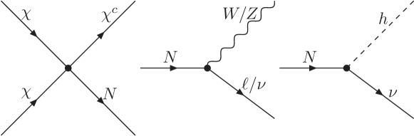
Figure 1: Feynman diagram of the semi-annihilation dark matter to RHN and the decays of RHN.

With Equation 2 & Equation 5 encapsulating all of the interactions of the $\chi$ and the $N_{i}$, their densities are essentially governed by the processes in Figure 1. The consequent Boltzmann equations are best represented as the evolution of the yield $Y$ ($Y\equiv n/s$ with $n$ being the number density of the species under consideration and $s$ the ambient entropy density) with the inverse of temperature, viz. $x\equiv m_{\chi}/T$. These can be summarised as (see Appendix C for a derivation)

$$\begin{array}[]{rcl}\displaystyle\frac{dY_{\chi}}{dx}&=&\displaystyle\frac{-x\,s(m_{\chi})}{2H(m_{\chi})}\sum_{i}\langle\sigma v\rangle^{\chi\chi\rightarrow\chi N_{i}}\left[Y_{\chi}^{2}-\frac{Y^{Eq}_{\chi}}{Y^{Eq}_{N}}Y_{\chi}\,Y_{N_{i}}\right],\\[12.91663pt] \displaystyle\frac{dY_{N_{i}}}{dx}&=&\displaystyle\frac{x\,s(m_{\chi})}{2H(m_{\chi})}\langle\sigma v\rangle^{\chi\chi\rightarrow\chi N_{i}}\left[Y_{\chi}^{2}-\frac{Y^{Eq}_{\chi}}{Y^{Eq}_{N}}Y_{\chi}\,Y_{N_{i}}\right]-\frac{\Gamma_{N_{i}}\,x}{H(m_{\chi})}(Y_{N_{i}}-Y_{eq})\ .\end{array}$$ (8)

Here, the thermally averaged cross-section DEramo:2017ecx is given by

$$\begin{array}[]{rcl}\displaystyle\langle\sigma(\text{ij}\rightarrow\text{kl})\,v\rangle&=&\displaystyle\left[4\,K_{2}(m_{i}/T)K_{2}(m_{j}/T)\,m_{i}^{2}\,m_{j}^{2}\,T\right]^{-1}\\[8.61108pt] &\times&\displaystyle\int^{\infty}_{E^{\text{min}}_{\rm cm}}dE_{\rm cm}\,\lambda(E^{2}_{\rm cm},m_{i},m_{j})\,\sigma_{\text{ij}\rightarrow\text{kl}}(E_{\rm cm})\,K_{1}(E_{\rm cm}/T)\end{array}$$ (9)

where $E_{\rm cm}$ is the center of mass energy, $K_{n}$ is the modified Bessel function of the second kind of order $n$ and $\lambda(a,b,c)$ is the usual Källen function. The expressions for the cross sections and the decay widths of the RHN can be gleaned from Appendix B.

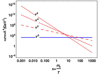
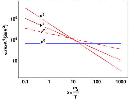
Figure 2: Different terms in expansion of $\langle\sigma v\rangle\times\Lambda^{4}$ plotted as a function of $x=m_{\chi}/T$ for SS interaction with a) $m_{\chi}=300{\rm GeV},m_{N}=100{\rm GeV}$ b) $m_{\chi}=1000{\rm GeV},m_{N}=100{\rm GeV}$.

A particular aspect needs to be appreciated at this juncture. It is commonplace to write $\langle\sigma v\rangle$ as a power series in the relative velocity $v$. In most scenarios, the terms involving the higher powers fall off quickly, allowing one to understand the scattering in terms of $s$-wave or $p$-wave dominance etc. In the present situation though, while the terms do continue to fall off similarly (see Figure 2), additional complications arise on account of the peculiarity of the effective interaction (and, thus, the amplitude). No single partial wave dominates over the entire range of evolution; rather, different terms can be important during the decoupling of DM, with the relative importance being a function of both the DM and the RHN masses. For example, as Figure 2 demonstrates, for a larger $m_{\chi}/m_{N}$, the $v^{2}$ term falls faster with $m_{\chi}/T$ whereas the $v^{6}$ term falls slower. Consequently, we use the full integral in Equation 9. The yield of dark matter, as of today, is well approximated by $Y_{\chi}(\infty)$ and can be used to calculate the relic abundance using

$$\Omega_{\chi}h^{2}=\displaystyle\frac{m_{\chi}s_{\infty}Y_{\chi}(\infty)h^{2}}{\rho_{c}}\ ,$$

where $s_{\infty}=2889.2\,\rm{cm}^{-3}$ and $\rho_{c}\,=\,1.05\,\times\,10^{-5}h^{2}\,\text{GeV}^{2}\text{ cm}^{-3}$.

       

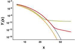
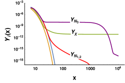
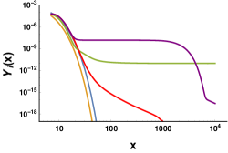
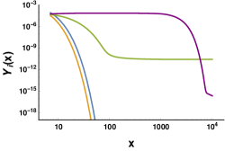
Figure 3: Yield of $\chi$ and right handed neutrino for $m_{\chi}=120,\Lambda=500,m_{N}=100$ as a function of $x\,=\,\frac{m_{\chi}}{T}$. The yellow and blue curves show the extrapolated equilibrium abundances of the DM and the RHN respectively. The green and red (purple) curves show the actual evolution of abundance of DM and RHN for different cases of Yukawa coupling: a) $y_{N_{i}}=(10^{-7},10^{-7},10^{-7})$, b) $y_{N_{i}}=(10^{-7},10^{-7},10^{-10})$, c) $y_{N_{i}}=(10^{-7},10^{-10},10^{-10})$ and d) $y_{N_{i}}=(10^{-10},10^{-10},10^{-10})$. The red and purple curves in b) and c) correspond to RHN with largest and smallest Yukawa couplings.

With the RHN playing a prime role in determining the DM relic abundance, it is imperative to examine the evolution of their density. The mass ratio $m_{N}/m_{X}$ as well as the size of the couplings, both play important roles resulting in a somewhat complicated behaviour as summarised in Figure 3, Here, the yields of the DM and the RHNs are shown as a function of $x=\frac{m_{\chi}}{T}$ for $m_{\chi}=120,\,m_{N_{i}}=100$ GeV and $\Lambda=500$ GeV. To highlight the individual epochs of freezing out, we employ a ruse wherein the yellow and blue curves represent the abundances of DM and RHN, respectively under the (unphysical) assumption of these never having fallen out of equilibrium. The actual evolution for the DM are depicted by the green curves while those for the RHN with $y_{N_{i}}=10^{-7}(10^{-10})$ are shown by the red(purple) ones.

At temperatures of the order of the electroweak scale, all the SM particles would, of course be in equilibrium. For $m_{N}\sim{\cal O}(100\,\mbox{GeV})$, a sizable $y_{N}\,(\sim 10^{-7})$ would ensure that the aforementioned decays of the $N_{i}$, along with the reverse processes, would keep these particles in equilibrium with the leptons and the weak bosons, and, hence with the entire SM sector. Furthermore, as the RHN are postulated to be lighter than the $\chi$, a large enough $y_{N_{i}}=10^{-7}$ (red curve) for all three RHNs, would imply that they would decouple at an epoch later than $\chi$ (green curve) and, hence, would have a much smaller relic density, as can be seen in Figure 3(a).

The situation changes dramatically if the $y_{N_{i}}$ is/are much smaller, as is illustrated by Figure 3(b) with $y_{N_{i}}=(10^{-7},10^{-7},10^{-10})$ and Figure 3(c) with $y_{N_{i}}=(10^{-7},10^{-10},10^{-10})$. While the densities of the $N_{i}$ with a larger Yukawa coupling (red curve) continue to behave as in Figure 3(a), those with small Yukawa coupling(s) (purple) behave differently as their interactions with the SM sector are now much weaker than the Hubble expansion rate. Hence, while the $N_{i}$ with larger Yukawas are still in equilibrium with the SM (and, through $\chi\chi\to\chi N$, so is the DM), these other RHNs decouple slightly before the DM does. Consequently, post decoupling, their number densities continue to be much larger than that of the DM. This has an interesting consequence. Owing to the larger density of such $N_{i}$, the process $\chi N_{i}\to\chi\chi$ would occur more frequently than the reverse, and the DM density would be slightly replenished before becoming constant at a slightly lower temperature. A careful comparison of Figure 3(b) and Figure 3(c) shows that this effect is more pronounced in the latter, which is but a consequence of the fact that the latter case corresponds to two $N_{i}$ with a small Yukawa coupling as opposed to just one for the former.

For the sake of illustration, in Figure 3(d) we depict the case where $y_{N_{i}}=(10^{-10},10^{-10},10^{-10})$, a situation that cannot explain all the neutrino masses. Owing to all the Yukawas being tiny, the RHN (purple) and, hence, the DM (green) both decouple from the equilibrium distribution very early. However, the tiny Yukawas also mean that the RHN decay late. Consequently, the $\chi N_{i}\to\chi\chi$ keeps on replenishing the DM relic abundance for a longer period.

With the sizes of the Yukawa couplings having such marked imprints on the thermal history, it is natural to expect that the relic densities too would be quite different. However, the dependence is not too severe as the value is primarily driven by $m_{\chi}$ and $\Lambda$. Indeed, on the scale of Figure 3, the differences do not show up. A careful calculation, though, shows that, in the four cases examined, $Y_{\chi}(x=10^{4})$ read $(a)\;4.4\times 10^{-12}$, $(b)\;8.15\times 10^{-12}$, $(c)\;9.7\times 10^{-12}$ and $(d)\;2.7\times 10^{-11}$, respectively.

We now turn to other consequences of the presence of the $N_{i}$. First and foremost, while their lifetimes are not ultrasmall, they still decay fast enough for overclosure to be an issue. On the other hand, their not so inconsiderable lifetimes could, presumably, alter physics at the era of big bang nucleosynthesis (BBN) or even the CMBR epoch. The latter alongwith the relative abundance of the light elements (BBN) encode information about the thermal history of the early universe, and is well described by SM physics. The decay of particles post such epochs have the potential of destroying the agreement between theoretical predictions and the observations. Fortunately though, in the present context, the longest lifetime of RHN is at most $0.001\,{\rm s}$ (corresponding to $y_{N}\sim 10^{-10}$ and $m_{N}\,=\,100\mathrm{\,Ge\kern-1.00006ptV\,}$) whereas BBN occured in the cosmic time window $0.1{\rm s}-10^{4}{\rm s}$ and CMB is even later. Thus, the abundance of RHN would have depreciated to a very large extent. To be quantitative, studies carried out in ref. Kawasaki:2017bqm show that the BBN constraints dictate that the fractional abundance of particles of mass ${\cal O}(100\mathrm{\,Ge\kern-1.00006ptV\,})$ and decaying into hadronically at $t\mathrel{\mathop{\kern 0.0pt\hbox to0.0pt{\raise 0.86108pt\hbox{$>$}\hss}}\lower 3.87495pt\hbox{\kern-1.90002pt$\sim$}}1\,{\rm s}$ after the inflationary phase should be less than $10^{-12}$. Thus, given the smallness of the $N_{i}$ lifetimes, BBN constraints are trivially satisfied. Similar is the case with the CMBR observations.

On the other hand, late decays of the $N$ would presumably leave their mark in the sky. The energetic neutrinos can be coming from RHN decay can be detected by experiments like SuperK, IceCube, etc Bandyopadhyay:2020qpn . However, such bounds are found to be much weaker compared to the ones coming from photon spectrum as discussed in section 4.

3.1 Scale and DM mass dependencies:

Having studied the various dependencies, we now proceed to determining the parameter space corresponding to the observed relic density. The various panels of Figure 4 depict the contours, in the $m_{\chi}-\Lambda$ plane satisfying $\Omega h^{2}=0.1199\pm 0.0012$ as applicable for different Lorentz structures of the effective 4-fermion interaction. Each panel corresponds to a different set of values for the Yukawa couplings $y_{N}$ with a common heavy neutrino mass $m_{N}$. Understandably, the area above the curves (larger $\Lambda$) corresponds to smaller interaction strengths and, hence, an overabundance of DM. On the other hand, the area below the curve leads to an under abundance and, hence, is still allowed (though only at the cost of postulating an additional component of the dark matter). Note that these results are obtained for $m_{\chi}\,>\,m_{N}$. For $m_{\chi}\,<\,m_{N}$, three body decays such as $N\to\nu+Z^{*}/h^{*}\to\nu\bar{f}f$ or $N\to\ell+W^{*}\to\ell\bar{f}f^{\prime}$ would be important. However, we do not explore this in the present work.

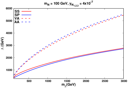
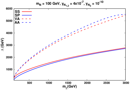
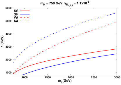
Figure 4: Contour on $m_{\chi}-\Lambda$ plane satisfying $\Omega h^{2}=0.1200\pm 0.0012$ for different interactions for different values of $m_{N}$ and $y_{N}$.

The curves in Figure 4 imply that obtaining the correct amount of energy density requires the mass of dark matter particles to increase with $\Lambda$. This could be easily understood by looking at the functional dependencies of the cross sections. With the DM particle being non-relativistic at the epoch of decoupling, the center of mass energy ($E_{\rm cm}$) for the process $\chi\chi\to\chi N$ is close to $2m_{\chi}$ and the thermal average of the cross section scales roughly as $m_{\chi}^{2}F(m_{N}/m_{\chi})/\Lambda^{4}$ where $F(m_{N}/m_{\chi})\,<\,1$ is specific to the form of the interaction Lagrangian. This immediately indicates that $\Lambda$ should scale roughly as $m_{\chi}^{2}$ with deviations depending on the form of $F(m_{N}/m_{\chi})$. Furthermore, that the $SS\,(\equiv PP)$ and $SP$ structures require a cut-off scale $\Lambda$ to be nearly half of what is required for $VA$ or $AA$ can be easily traced to the fact that the two disparate sets of cross sections differ by a factor of nearly 16.

As for the $m_{N}$ dependence, note that for the VA and SP structures, $F(m_{N}/m_{\chi})$ is a monotonically decreasing function of the argument. The consequent decrease in the total cross section with an increase in $m_{\chi}$ would need to be compensated by an associated decrease in $\Lambda$ so as to lead to an unchanged relic abundance, and this is reflected in a comparison of panels $(a),(c)$ and $(d)$ of Figure 4. On the other hand, for the SS and AA cases, the cross sections do not change appreciably with $m_{N}$.

Finally, Figure 4(b) corresponds to the case where one of the RHN has small decay width ($y_{N_{i}}=10^{-7},10^{-7},10^{-10}$), which leads to a nominally larger relic abundance (as shown in Figure 3(b)) as compared to the case where all the RHNs have same Yukawa coupling, $y_{N_{i}}=10^{-7}$.

Before we end this section, it is contingent upon us to examine the validity of the effective field theory paradigm vis á vis the parameter space required to satisfy the correct relic density. Clearly, the cut-off scale $\Lambda$ for such a description must be larger than the masses of any particle present in the theory. In the present case, this is definitely satisfied by the entire parameter space for the VA and the AA cases. For the (pseudo) scalar current-current structures, though, this is not so for larger $m_{\chi}$ values (although, for smaller $m_{\chi}$, this does hold). In other words, the effective theory approach may not be entirely valid and the use of the full theory seems to be called for. It is, however, easy to ascertain that the consequent changes in this part of the analysis would not be severe, and that the results obtained herein are precise enough for an exploratory study that this is.

4 Constraints from indirect detection of DM

The semi-annihilations of the DM would also lead to electrons, positrons, quarks, neutrinos, gamma-rays etc. with different energy spectra. Of these, gamma-ray observations have been used prominently to probe the presence of DM decay, annihilations and semi-annihilations. The reasons for the choice are twofold: $\gamma-$ray emissions from various astrophysical objects are well understood, and unlike charged particles, photons travel through interstellar and intergalactic matter suffering relatively little obstruction. Thus, by comparing the expected gamma-ray flux to the measured one, one can derive upper limits on DM interactions in the absence of any excess.

The processes relevant to the present study is the semi-annihilation of DM to RHN which, subsequently, decay via $W^{\pm}\ell,\,Z\nu$ and $h\nu$ with the bosons cascading down to quarks (hadronizing almost instantly) and leptons. The resultant charged particles from the decay yield gamma rays, either during hadronization or as a result of final state radiation processes. To this end, we use observations from the following three experiment set-ups to constrain the effective operators analysed in this work:

• Fermi-LAT: The satellite covers a wide energy range, starting from $0.5$ GeV and going up to $0.5$ TeV. To derive the exclusion limits, 6 years of data from 15 dwarf Spheroidals (see Table 1 of fermilat ), based on the pass 8 event analysis fermilat is used.

• The High Energy Stereoscopic System (H.E.S.S.) is sensitive to high energy $\gamma-$rays spanning energies ranging from $0.2$ TeV to 30 TeV. The initial phase (H.E.S.S. I) had already published competitive limits on DM annihilations cross sections HESS:2011zpk . With the addition of a large dish at the center of the array, the second phase (H.E.S.S. II) is expected to lead to much stronger constraints HESS . To exploit this expected sensitivity, we first tune our analysis to reproduce the H.E.S.S I data HESS:2011zpk , and follow it by rescaling it with the projected sensitivity in the $b\bar{b}$ channel as calculated in Ref.HESS .

• With more than a 100 individual telescopes, the Cherenkov Telescope Array (CTA) would be well-placed to detect high-energy gamma-rays over a very wide energy range ($\sim$60 GeV to $\sim$300 TeV) and is projected to be more than ten times as sensitive as the currently operating ones. This unprecedented sensitivity is expected to yield very strong constraints (if not an actual discovery) especially when looking at gamma-rays from Galactic center.

Note that the Fermi-LAT experiment is more sensitive to gamma-rays at low energies, whereas H.E.S.S. and CTA are sensitive at larger energies.

4.1 The $\gamma$–ray spectrum:

A gamma-ray signal from DM annihilation or semi annihilation is inferred from the number of photons at a given energy bin from a portion of the sky. The quantity that captures this information is the differential flux, which is proportional to: $(i)$ the square of the number density of the dark matter particle; $(ii)$ the thermal-averaged product of the annihilation cross-section and the velocity ($\langle\sigma v\rangle$); $(iii)$ the number of photons produced per dark matter process as a function of energy, i.e the energy spectrum (dN/dE); and $(iv)$ the size and density of the region of the sky under study, as captured in the $J$-factor. On inclusion of the appropriate normalization factor, the differential flux for dark matter semi-annihilation is

$$\frac{d\phi_{\gamma}}{dE}=\frac{1}{8\pi m_{\chi}^{2}}\langle\sigma v\rangle\frac{dN_{\gamma}}{dE}J,$$ (10)

where

$$J=\int_{l.o.s}\frac{ds}{r_{\odot}}\left(\frac{\rho(r(s,\theta))}{\rho_{\odot}}\right)^{2},$$ (11)

and includes an integration over the line-of-sight between the observatory and the source. This factor obviously depends on the dark matter distribution which we have assumed to follow the NFW profile Navarro:2008kc .

Figure 5: Photon energy spectrum for different values of $m_{\chi}$ at a fixed value of $m_{N}\,=\,100$ GeV.

We compute the energy spectrum $dN/dE$ due to the semi-annihilation processes etc., including the hadronization effects, using a suitably augmented version of PYTHIA8.3 Sjostrand:2014zea . The resultant normalised energy spectrum for different values of $m_{\chi}$ at a fixed RHN mass (with the RHN decaying to a final state containing an $e^{\pm}$) in Figure 5. Since the DM is non-relativistic, the energy of the RHN can be estimated to be

$$E_{N}\,=\,\displaystyle\frac{s+m_{N}^{2}-m_{\chi}^{2}}{2\sqrt{s}}\sim\displaystyle\frac{m_{N}^{2}+3m_{\chi}^{2}}{4m_{\chi}}\ .$$

As expected, and as illustrated by Figure 5, a heavier DM leads to a more energetic RHN. With the extra energy being transmitted to the $N$’s decay products, this would lead to a harder gamma-ray spectrum. Given the expression for $E_{N}$, it is obvious that it changes substantially with $m_{N}$ only when the latter is comparable to $m_{\chi}$. This property is naturally transmitted to the $N$’s daughters, including to the gamma-ray spectrum (Figure 6). For a given $m_{\chi}$, the heaviest of the $N$s would lead to the hardest $\gamma$–spectrum. On the other hand, by virtue of being most boosted, the lighter ones lead to a larger number of energetic photons (Figure 6). Finally, for a given $(m_{\chi},m_{N})$ combination, with each being heavier than a 100 GeV, the leptons from the $N$’s decay would have a virtually flavour-independent energy spectrum. Nonetheless, the $\tau$-channel would result in more energetic photons owing simply to its decay and subsequent hadronization. Understandably, the spectrum for the muonic decay channel would lie in between the two.

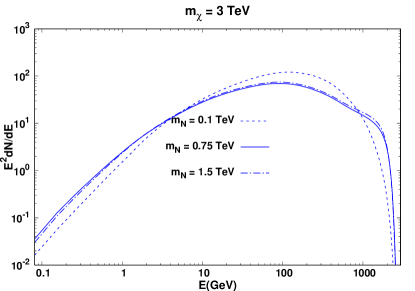
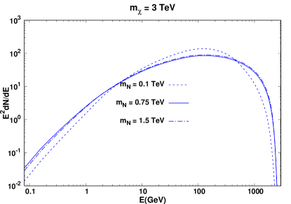
Figure 6: Photon energy spectrum for $m_{\chi}\,=\,3$ TeV for different values of RHN mass and different final state leptons (a) electron and (b) tau-lepton.

4.2 Results

Armed with the discussions of the preceding subsection, we are now in a position to compare the expectations of our model with the observational data from Fermi-LAT and H.E.S.S. on the one hand, and compare with the expected sensitivity of the CTA on the other. To this end, we use the GamLike package GAMBIT to compute the likelihood function $\mathcal{L}(\hat{\mu},\hat{\theta}|\mathcal{D})$ where $\mathcal{D}$ represents the observational data, $\hat{\theta}$ the (unknown) parameters describing the background and $\hat{\mu}$ a set of parameters encapsulating the features of the dark matter model. The limits on the semi-annihilation cross-section are then derived through the statistical test (TS),

$$TS=-2\ln{\left(\frac{\mathcal{L}(\hat{\mu}_{0},\hat{\theta}|\mathcal{D})}{\mathcal{L}(\hat{\mu},\hat{\theta}|\mathcal{D})}\right)},$$ (12)

with $TS>2.71$ corresponding to $95\%$ C.L. exclusion. Here, $\hat{\mu}_{0}$ corresponds to the null hypothesis, i.e., the absence of dark matter.

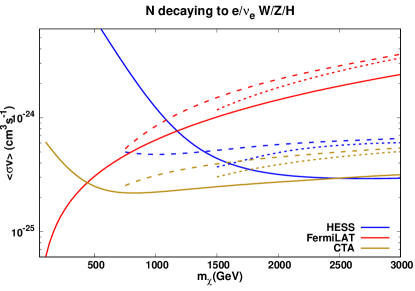
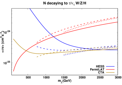
Figure 7: Upper limits on $\langle\sigma v\rangle$ as a function of $m_{\chi}$ for a) electron-RHN final state and b) tau-RHN final state. We obtained these limits from different experiments Fermi-LAT, H.E.S.S. and CTA for different values of RHN mass, $m_{N}\,=\,100$ GeV (Solid), $m_{N}\,=\,750$ GeV (dashed) and $m_{N}\,=\,1500$ GeV (dotted).

The consequent constraints, in the $m_{\chi}$–$\langle\sigma v\rangle$ plane, from the Fermi-LAT and H.E.S.S. as also the projected CTA sensitivity are depicted in Figure 7. The area above the curves are (would be) ruled out at 95% C.L. Understandably, the limits for the tau–channel are slightly more stringent as it leads to a slightly larger gamma-ray production. As pointed out earlier, the FermiLAT experiment is more sensitive at lower energies, whereas H.E.S.S. is sensitive in the $0.2-30$ TeV range. Similarly, the energy threshold of the CTA is lower than that of H.E.S.S., making the CTA much more sensitive to photons of intermediate energies. Thus, CTA would furnish the strongest bounds for dark matter masses above 600 GeV almost independent of $m_{N}$, whereas the FermiLAT gives better limits for $m_{\chi}\mathrel{\mathop{\kern 0.0pt\hbox to0.0pt{\raise 0.86108pt\hbox{$<$}\hss}}\lower 3.87495pt\hbox{\kern-1.90002pt$\sim$}}500\mathrm{\,Ge\kern-1.00006ptV\,}$. For $m_{\chi}$ greater than a few TeV, H.E.S.S. already provides bounds equally significant as as those the CTA would lead to.

The shape of the constraint curves are determined by a convolution of the $\gamma$-ray spectrum with the energy sensitivity. To understand the final outcome, several aspects have to be borne in mind:

• As we have discussed earlier, the three detectors have peak sensitivity at different $E_{\gamma}$ ranges. Fermi-LAT is the most sensitive at lower energies (0.5 GeV to 0.5 TeV) while for H.E.S.S,, this lies in the few TeVs range. As for the CTA, although it covers a very wide range ($\sim$60 GeV to $\sim$300 TeV), for low-energy (in tens of GeVs) $\gamma$-rays it obviously loses out to Fermi-LAT. For somewhat higher energies, it competes very will with the H.E.S.S., and goes much beyond.

• Thus, we would expect the Fermi-LAT to be the most sensitive detector for relatively low DM masses, as is borne out by Figure 7.

• Naively, one would expect that a larger value for $m_{N}$ would, typically, translate to more energetic decay products and, hence, a harder $\gamma$-ray spectrum. Consequently, the constraints from non-observation would be stronger. This is reflected by the fact of the constraints being stronger for $m_{N}=1.5$ TeV than they are for $m_{N}=0.75$ TeV. This argument, though, fails for the $m_{N}=100$ GeV case.

• For $m_{N}\ll m_{\chi}$, the RHN is highly boosted and this is transferred to its daughters, thereby allowing them to radiate off more photons. Some of these would have energies between 20 GeV and 0.5 TeV and visible to the detectors under discussion. With Fermi-LAT’s sensitivity to low energy $\gamma$-rays being the highest, the improvement is most pronounced for this case.

Compared to DM annihilation Campos:2017odj ; Jangid:2020qgo these indirect bounds are less constrained for the semi-annihilation processes semianniSca1 , as expected owing to less photon in the final state.

We also analysed the sensitivity of semi-annihilating DM through their neutrino spectrum in detectors like Super-kamiokande Super-Kamiokande:2015qek . We found that the limits are atleast $\mathcal{O}(1)$ magnitude weaker than the DM annihilating to two neutrinos Arguelles:2019ouk and 2-3 orders of magnitude weaker than the complimentary photon channel discussed above. This is due to the fact that the neutrino spectrum is weaker in comparison to photon spectrum and additionally, neutrinos interact weakly with the detectors. Thus, a dedicated analyses that include direction and energy information might provide the stronger limits. Similarly, neutrino experiments/detectors like DUNE DUNE:2020ypp and Hyper-Kamiokande Olivares-DelCampo:2018pdl can provide stronger limits for low-$\chi$ whereas IceCube IceCube:2016oqp and ANTARES ANTARES:2015vis can be utilized for heavy-$\chi$. Even so, these are expected to be weaker than the complementary photon channel.

Before end this section we would like to comment on the fact that semi-annihilation processes inn an effective theory does not have mediator to couple to the nucleons, thus do not put any direct detection constraints. However, for an UV complete theory as discussed in Appendix A can lead to the restriction on nucleon-DM couplings.

5 Conclusion

The continued absence of any signal for particulate Dark Matter, other than the astrophysical or cosmological inferences calls for a reevaluation of the paradigm. One particular aspect is the mechanism that renders it stable against decay. While in most theories, this is ensured by the imposition of a $Z_{2}$ symmetry, it certainly is not the only avenue. Alternatives such as $Z_{n}\,(n>2)$, or even more complicated ones, are not only feasible, but also dramatically alter the expectations in both laboratory (direct detection) as well as satellite-bound (indirect detection) experiments.

In this study we consider the simplest alternative, namely a $Z_{3}$ symmetry under which the DM $\chi$ transforms nontrivially while all the Standard Model fields transform trivially. While similar efforts have been made earlier for scalar DM, we eschew that path for every new fundamental scalars brings along its own hierarchy problem. Instead, we choose to work with a fermionic DM.

We further augment the theory by the inclusion of right-handed (SM- as well as $Z_{3}$ neutral) neutrino fields $N_{i}$. These serve twin purposes. Allowed Majorana masses as well as nonvanishing Yukawa couplings connecting with the SM neutrinos, they allow the generation of correct masses for the light neutrinos (via the seesaw mechanism). Furthermore, they offer an efficient avenue for the disappearance of the DM so as to obtain the correct relic density.

Rather than adopt a particular UV-complete theory (although we do offer one in an Appendix), we have chosen to work in the effective theory framework (with a cutoff scale $\Lambda$) through the inclusion of dimension-six operators involving $\chi$ and the $N_{i}$. While complete annihilations ($\bar{\chi}+\chi\to N_{i}+N_{j}$) are possible, for a very wide range of parameters (as exemplified in the Appendix), it is the semi-annihilation process ($\chi+\chi\to\chi^{c}+N_{i}$) that dominates.

The Boltzmann equations governing the evolution of the DM density changes from the usual paradigm not only because it is the semi-annihilation that dominates, but also because it is coupled with the evolution of the $N_{i}$ densities, which decay to the SM particles through their Yukawa couplings. If the size of these couplings are to be commensurate with the observed neutrino masses, they do help in keeping the $N_{i}$ in equilibrium with the SM plasma until relatively late. The exact sizes of these couplings understandably have a very big effect on the $N_{i}$ decoupling era and, hence, their densities at that epoch. However, the effect on the $\chi$ relic density is not as pronounced. Given this, we have obtained the region in the EFT parameter space that correctly reproduces the relic density for various choices of the operators in the effective Lagrangian. On the adoption of a specific UV-complete theory (as in Appendix A), this can be easily translated to a corresponding statement for the said theory.

While direct detection experiments would obviously be insensitive to such a scenario, the indirect detection theatre is a very interesting one. The decays of the $N_{i}$ (themselves the products of the semi-annihilation process) yield charged particles (gauge bosons/quarks and charged leptons). These, as well as their cascade decay products, radiate energetic photons which could be detected by the satellite experiments like FermiLAT or earth based telescope like the H.E.S.S. and CTA. We explored such detection possibilities in detail, simulating the photon energy spectrum and convoluting with the detector responses. While non-observation of such signals the Fermi-LAT already imposes interesting bounds, especially for a light DM, future data from H.E.S.S.-II and the CTA are expected to lead to strong bounds in the the heavy-$\chi$ region. As an example, for $m_{\chi}\sim\,100{\,\rm GeV}$, a thermal annihilation cross section $\langle\sigma v\rangle\sim 5\times 10^{-26}{\rm cm}^{3}{\rm s}^{-1}$ would be ruled out. For heavier $m_{\chi}$, the bounds are weaker, and most of the parameter space satisfying relic abundance is allowed by the Fermi-LAT, H.E.S.S and C.T.A data. And although, the neutrino spectrum of RHN’s, can, in principle, be detected in several neutrino detectors, the corresponding constraints are much weaker compared to those obtained from the gamma-ray telescopes.

With the effective theory presented here easily escaping constraints from current and near-future experiments, it is obvious that such a scenario can indeed alleviate the tension between the Planck measurements of the DM relic density on the one hand and the null results from direct and indirect detections of DM on the other. It also needs to be appreciated that the quest for an UV complete theory (such as that discussed in Appendix A) could engender DM-nucleon interactions as well as self-interactions of the DM. While the former would open new windows to both direct and indirect detection, the latter could be expected to leave a discernible mark on the small-scale structure in galaxies and clusters. The paradigm, thus, holds much promise.

Appendix A An ultraviolet completion

While the Lagrangian of (Equation 5) is quite acceptable as an effective theory, a renormalizable theory is always desirable. Furthermore, the absence of certain terms (such as $\bar{\chi}\Gamma_{i}\chi\,\bar{N}\Gamma_{j}N$, with $\Gamma_{i,j}$ being commensurate Dirac matrices) in (Equation 5) is a cause of concern for their presence would tend to reduce the efficacy of semi-annihilation. In this Appendix, we present a possible ultraviolet completion that addresses both these issues.

To this end, let us introduce, to the model in section 2, a $SU(2)_{L}$ singlet neutral scalar $\phi$ which transforms, under $Z_{3}$, just as $\chi$ does. This would allow for Yukawa terms of the form

$$L_{int}\supset\bar{\chi^{c}}\left(y_{2}+y_{2}^{\prime}\gamma_{5}\right)\chi\phi+\phi\,\bar{\chi}\left(y_{3}+y_{3}^{\prime}\gamma_{5}\right)\,N+\text{H.c.}$$ (13)

In the event of a heavy $\phi$, the field can be integrated out to yield effective four-fermion vertices of the form $(C_{ab}/m_{\phi}^{2})\,\left(\bar{N}\Gamma_{a}\chi\right)\left(\bar{\chi^{c}}\Gamma_{b}\chi\right)$ with the coefficients $c_{ab}$ being related through Fierz rotations.

Of course, analogous terms such as $\bar{\chi}\Gamma_{i}\chi\,\bar{N}\Gamma_{j}N$ would be generated as well. However, for $|y_{3},y_{3}^{\prime}|\ll|y_{2},y_{2}^{\prime}|$ — a technically natural choice — such operators are relatively suppressed with the consequence that semi-annihilation wins over annihilation.

It is instructive to consider the potential for the scalars in the theory, namely $\phi$ and the usual SM doublet $\Phi$. The most general form is given by

$$V(\Phi,\phi)=\mu_{1}^{2}|\Phi|^{2}+\mu_{2}^{2}|\phi|^{2}+\frac{\mu_{3}}{3}\left(\phi^{3}+\phi^{\dagger 3}\right)+\frac{\lambda_{1}}{2}|\Phi|^{4}+\frac{\lambda_{2}}{2}|\phi|^{4}+\lambda_{\phi}|\phi|^{2}|\Phi|^{2}+\text{H.c.}$$ (14)

A nonzero value for $\langle\phi\rangle$ would result in $\phi-\Phi$ mixing, and thereby to direct $\chi\chi$ annihilation to the SM particles through the Higgs portal. However, the spontaneous breaking of $Z_{3}$ that this entails would also allow the DM to decay. While the lifetime could be suitably extended by choosing parameters appropriately, the solutions tend to be somewhat unnatural and we eschew that path.

Appendix B Getting to the cross sections

We list below the squares of the matrix elements for the process in Equation 7 using the Lagrangian of Equation 5 with the assumption that only one of the $c_{ab}$ is non-zero and set to unity. Defining the Lorentz-invariant quantities

$$\begin{array}[]{rcl}{\cal A}_{4}&\equiv&\displaystyle q_{1}\cdot q_{3}\,q_{2}\cdot q_{4}+q_{1}\cdot q_{2}\,q_{3}\cdot q_{4}+q_{1}\cdot q_{4}\,q_{2}\cdot q_{3}\\[4.30554pt] {\cal A}_{2}&\equiv&\displaystyle q_{1}\cdot q_{3}+q_{2}\cdot q_{3}+q_{3}\cdot q_{4}\\[4.30554pt] \widetilde{\cal A}_{2}&\equiv&\displaystyle q_{1}\cdot q_{2}+q_{1}\cdot q_{4}+q_{2}\cdot q_{4}\end{array}$$ (15)

we have

$$\begin{array}[]{rcl}\displaystyle|M|^{2}_{SS}=|M|^{2}_{PP}&=&\displaystyle\frac{8}{\Lambda^{4}}\left({\cal A}_{4}-m^{2}\,{\cal A}_{2}+mm_{N}\,\widetilde{\cal A}_{2}-3m^{3}m_{N}\right)\\[8.61108pt] |M|^{2}_{SP}\,=|M|^{2}_{PS}&=&\,\displaystyle\frac{8}{\Lambda^{4}}\left(-{\cal A}_{4}+m^{2}\,{\cal A}_{2}+mm_{N}\,\widetilde{\cal A}_{2}-3m^{3}m_{N}\right)\\[8.61108pt] |M|^{2}_{VV}&=&\,\displaystyle\frac{128}{\Lambda^{4}}\left({\cal A}_{4}+\frac{m^{2}}{2}\,{\cal A}_{2}-\frac{mm_{N}}{2}\,\widetilde{\cal A}_{2}-3m^{3}m_{N}\right)\\[8.61108pt] |M|^{2}_{VA}&=&\,\displaystyle\frac{128}{\Lambda^{4}}\left({\cal A}_{2}-m^{2}\,{\cal A}_{2}-mm_{N}\,\widetilde{\cal A}_{2}+3m^{3}m_{N}\right)\\[8.61108pt] |M|^{2}_{AA}&=&\,\displaystyle\frac{128}{\Lambda^{4}}\left({\cal A}_{4}-m^{2}\,{\cal A}_{2}+mm_{N}\,\widetilde{\cal A}_{2}-3m^{3}m_{N}\right)\end{array}$$ (16)

Note that spin-summing (and averaging) is yet to be done. The corresponding expressions for the reverse process ($\bar{\chi}^{c}\to\chi\chi$) or analogous ones (such as $\chi N\to\chi^{c}\chi^{c}$ etc.) can be obtained from those above using crossing symmetry.

Similarly, the decay widths for the RHN are given by

$$\begin{array}[]{rclcl}\displaystyle\Gamma(N_{i}\to W^{+}l^{-})&=&\displaystyle\Gamma(N_{i}\to W^{-}l^{+})&=&\displaystyle\frac{y_{N}^{2}M_{N_{i}}}{32\pi}\left(1-\frac{M_{W}^{2}}{M_{N_{i}}^{2}}\right)^{2}\left(1+\frac{2M_{W}^{2}}{M_{N_{i}}^{2}}\right),\\[15.0pt] \displaystyle\Gamma(N_{i}\to Z\,\nu)&=&\displaystyle\Gamma(N_{i}\to Z\,\bar{\nu})&=&\displaystyle\frac{y_{N_{i}}^{2}M_{N_{i}}}{64\pi}\left(1-\frac{M_{Z}^{2}}{M_{N_{i}}^{2}}\right)^{2}\left(1+\frac{2M_{Z}^{2}}{M_{N_{i}}^{2}}\right).\\[15.0pt] \displaystyle\Gamma(N_{i}\to h\,\nu)&=&\displaystyle\Gamma(N_{i}\to h\,\bar{\nu})&=&\displaystyle\frac{y_{N_{i}}^{2}M_{N_{i}}}{64\pi}\left(1-\frac{M_{h}^{2}}{M_{N_{i}}^{2}}\right)^{2}.\end{array}$$ (17)

where the masses of the charged leptons have been neglected.

Appendix C Boltzmann Equation

We, now, derive the Boltzmann equation relevant for the Dark Matter density evolution in the present context. With $2\to 2$ scattering being the dominant process, the calculation proceeds quite similarly to the standard case, except for the fact that only one DM particle is produced (or destroyed) per collision process. On the other hand, there would be two identical particles in either the initial or the final state, thereby necessitates the inclusion of a factor of $(1/2!)$ in the phase space calculation. This gives, for the $1+2\to 3+4$ process, the time-variation of the number density $n_{\chi}$ to be

$$\begin{array}[]{rcl}\displaystyle\frac{dn_{\chi}}{dt}\,+\,3Hn_{\chi}&=&\displaystyle\,\frac{-1}{2!}\int\left[d{\cal P}\right]\Big{(}|M_{12\to 34}|^{2}f_{1}f_{2}-|M_{34\to 12}|^{2}f_{3}f_{4}\Big{)}\end{array}$$ (18)

where, for the sake of simplicity, we have suppressed the Pauli blocking factors. Here, $f_{i}$s represent the appropriate statistical distribution factors, $H$ is the instantaneous Hubble expansion rate and

$$[d{\cal P}]\equiv\left(\prod_{i=1}^{4}\frac{d^{3}p_{i}}{(2\pi)^{3}2E_{i}}\right)\,(2\pi)^{4}\delta^{4}(p_{1}+p_{2}-p_{3}-p_{4})$$ (19)

with appropriate spin-sum and averaging being understood. If we assume time-reversal invariance, we have $|M_{12\to 34}|^{2}=|M_{34\to 12}|^{2}$ and, thus, the right hand side of eqn. 18 can be written as

$$\text{R.H.S}\,=\,\frac{-1}{2}\int\left[d{\cal P}\right]|M_{12\to 34}|^{2}\left(f_{1}f_{2}-f_{3}f_{4}\right)\ .$$ (20)

Rather than continue with the number density $n_{\chi}$, it is customary to consider the yield which is defined as it ratio with the ambient entropy density $s$, viz. $Y_{\chi}\equiv n_{\chi}/s.$ This immediately leads to

$$\frac{dn_{\chi}}{dt}\,+\,3Hn_{\chi}\,=\,s\frac{dY_{\chi}}{dt}\ .$$

Noting that, during the cosmological evolution, there exists a monotonic relation between the time elapsed and the temperature of the universe, it is useful to consider a change of variables

$$x=\frac{m_{\chi}}{T}$$

such that we have

$$\frac{dY_{\chi}}{dx}=\frac{-x}{2H(m_{\chi})s}\int\left[d{\cal P}\right]$$ (21)

where

$$H(m_{\chi})\,=\,\displaystyle\frac{\pi\sqrt{g_{*}}m_{\chi}^{2}}{\sqrt{90}M_{\text{pl}}}\qquad{\rm and}\qquad s\,=\,\displaystyle\frac{2\pi^{2}g_{*}T^{3}}{45}\,=\,\frac{2\pi^{2}g_{*}m_{\chi}^{3}}{45x^{3}}\ .$$

with $g_{*}$ denoting the number of degrees of freedom relevant at that temperature.

It is an excellent approximation to consider these particles $(N$ and $\chi$) to be in kinetic equilibrium during the freeze out. This allows us to write

$$f(E,t)=\frac{n(x)}{n^{\text{eq.}}(x)}f^{\text{eq.}}(E,t)$$

where

$${f^{\text{eq.}}\,=\,\frac{1}{e^{E/T}+1}\qquad\text{and}\qquad n^{\text{eq.}}\,=\,\displaystyle\frac{g}{2\pi^{2}}\int_{m}^{\infty}\frac{(E^{2}-m^{2})^{1/2}}{e^{E/T}+1}E\,dE}$$

both $\chi$ and $N_{i}$ being fermionic. Now, decoupling occurs, typically, at $x\equiv m_{\chi}/T\mathrel{\mathop{\kern 0.0pt\hbox to0.0pt{\raise 0.86108pt\hbox{$>$}\hss}}\lower 3.87495pt\hbox{\kern-1.90002pt$\sim$}}20$ and, hence, in $f^{\text{eq}}(\chi)$, we may safely approximate $(e^{E/T}+1)^{-1}\approx e^{-E/T}$. And, since we would not be contemplating a large hierarchy between $m_{\chi}$ and $m_{N}$, an analogous approximation would hold as well for $f^{\text{eq}}(N_{i})$. Furthermore, using conservation of energy, we have

$$f^{\text{eq.}}_{1}(x)f^{\text{eq.}}_{2}(x)\approx e^{-(E_{1}+E_{2})/T}\,=\,e^{-(E_{3}+E_{4})/T}\approx f^{\text{eq.}}_{3}(x)f^{\text{eq.}}_{4}(x)$$ (22)

This leads to

$$\begin{array}[]{rcl}\displaystyle\frac{dY_{\chi}}{dx}&=&\displaystyle\frac{-x}{2H(m)s}\int\left[d{\cal P}\right]|M_{12\to 34}|^{2}\Bigg{[}\frac{n_{1}(x)n_{2}(x)}{n^{\text{eq.}}_{1}(x)n^{\text{eq.}}_{2}(x)}f^{\text{eq.}}_{1}(E,t)f^{\text{eq.}}_{2}(E,t)\\[12.91663pt] &&\displaystyle\hskip 120.00018pt-\frac{n_{3}(x)n_{4}(x)}{n^{\text{eq.}}_{3}(x)n^{\text{eq.}}_{4}(x)}f^{\text{eq.}}_{3}(E,t)f^{\text{eq.}}_{4}(E,t)\Bigg{]}\\[17.22217pt] &=&\displaystyle\frac{-x}{2H(m)s}\int\left[d{\cal P}\right]\frac{|M_{12\to 34}|^{2}}{n^{\text{eq.}}_{1}(x)n^{\text{eq.}}_{2}(x)}f^{\text{eq.}}_{1}(E,t)f^{\text{eq.}}_{2}(E,t)\\[12.91663pt] &&\displaystyle\hskip 60.00009pt\left[n_{1}(x)n_{2}(x)-n_{3}(x)n_{4}(x)\frac{n^{\text{eq.}}_{1}(x)n^{\text{eq.}}_{2}(x)}{n^{\text{eq.}}_{3}(x)n^{\text{eq.}}_{4}(x)}\right]\\[17.22217pt] &=&\displaystyle\frac{-x\,s}{2H(m)}\int\left[d{\cal P}\right]\frac{|M_{12\to 34}|^{2}}{n^{\text{eq.}}_{1}(x)n^{\text{eq.}}_{2}(x)}f^{\text{eq.}}_{1}(E,t)f^{\text{eq.}}_{2}(E,t)\\[12.91663pt] &&\displaystyle\hskip 60.00009pt\left[Y_{1}(x)Y_{2}(x)-Y_{3}(x)Y_{4}(x)\frac{Y^{\text{eq.}}_{1}(x)Y^{\text{eq.}}_{2}(x)}{Y^{\text{eq.}}_{3}(x)Y^{\text{eq.}}_{4}(x)}\right]\ .\end{array}$$

Thus, defining a thermal average as

$$\langle\sigma v\rangle\equiv\int\left(\prod_{i=1}^{4}d\Pi_{i}\right)\frac{(2\pi)^{4}\delta^{4}(p_{1}+p_{2}-p_{3}-p_{4})}{n^{\text{eq.}}_{1}(x)n^{\text{eq.}}_{2}(x)}|M_{12\to 34}|^{2}f^{\text{eq.}}_{1}(E,t)f^{\text{eq.}}_{2}(E,t)\ ,$$

we obtain the set of equations describing the evolution of number density of DM as well as RHN in the early universe:

$$\begin{array}[]{rcl}\displaystyle\frac{dY_{\chi}}{dx}&=&\displaystyle\frac{-x\,s(m_{\chi})}{2H(m_{\chi})}\langle\sigma v\rangle^{\chi\chi\rightarrow\chi N}\left[Y_{\chi}^{2}-\frac{Y^{Eq}_{\chi}}{Y^{Eq}_{N}}Y_{\chi}\,Y_{N}\right]\\[17.22217pt] \displaystyle\frac{dY_{N}}{dx}&=&\displaystyle\frac{x\,s(m_{\chi})}{2H(m_{\chi})}\langle\sigma v\rangle^{\chi\chi\rightarrow\chi N}\left[Y_{\chi}^{2}-\frac{Y^{Eq}_{\chi}}{Y^{Eq}_{N}}Y_{\chi}\,Y_{N}\right]-\frac{\Gamma_{N}\,x}{H(m_{\chi})}(Y_{N}-Y_{eq})\ .\end{array}$$ (23)

Note that the second term in $dY_{N}/dx$ carries the information of the RHN decaying into the SM particles.

References

- [1] P. Minkowski, Phys. Lett. B 67 (1977), 421-428 doi:10.1016/0370-2693(77)90435-X
- [2] J. Schechter and J. W. F. Valle, Phys. Rev. D 22 (1980), 2227 doi:10.1103/PhysRevD.22.2227
- [3] R. N. Mohapatra and G. Senjanovic, Phys. Rev. D 23 (1981), 165 doi:10.1103/PhysRevD.23.165
- [4] R. N. Mohapatra and G. Senjanovic, Phys. Rev. Lett. 44 (1980), 912 doi:10.1103/PhysRevLett.44.912
- [5] T. Yanagida, Prog. Theor. Phys. 64 (1980), 1103 doi:10.1143/PTP.64.1103
- [6] A. Falkowski, J. Juknevich and J. Shelton, [arXiv:0908.1790 [hep-ph]].
- [7] V. González-Macías, J. I. Illana and J. Wudka, JHEP 05 (2016), 171 doi:10.1007/JHEP05(2016)171 [arXiv:1601.05051 [hep-ph]].
- [8] M. Escudero, N. Rius and V. Sanz, Eur. Phys. J. C 77 (2017) no.6, 397 [arXiv:1607.02373 [hep-ph]].
- [9] Y. Tang and S. Zhu, JHEP 01 (2017), 025 [arXiv:1609.07841 [hep-ph]].
- [10] M. D. Campos, F. S. Queiroz, C. E. Yaguna and C. Weniger, JCAP 07 (2017), 016 [arXiv:1702.06145 [hep-ph]].
- [11] B. Batell, T. Han and B. Shams Es Haghi, Phys. Rev. D 97 (2018) no.9, 095020 [arXiv:1704.08708 [hep-ph]].
- [12] M. Blennow, E. Fernandez-Martinez, A. Olivares-Del Campo, S. Pascoli, S. Rosauro-Alcaraz and A. Titov, Eur. Phys. J. C 79, no.7, 555 (2019) [arXiv:1903.00006 [hep-ph]].
- [13] E. Hall, T. Konstandin, R. McGehee and H. Murayama, [arXiv:1911.12342 [hep-ph]].
- [14] P. Bandyopadhyay, E. J. Chun, R. Mandal and F. S. Queiroz, Phys. Lett. B 788 (2019), 530-534 doi:10.1016/j.physletb.2018.12.003 [arXiv:1807.05122 [hep-ph]].
- [15] P. Bandyopadhyay, E. J. Chun and R. Mandal, Phys. Rev. D 97 (2018) no.1, 015001 doi:10.1103/PhysRevD.97.015001 [arXiv:1707.00874 [hep-ph]].
- [16] P. Bandyopadhyay, E. J. Chun and J. C. Park, JHEP 06 (2011), 129 doi:10.1007/JHEP06(2011)129 [arXiv:1105.1652 [hep-ph]].
- [17] P. Bandyopadhyay, E. J. Chun and R. Mandal, JCAP 08 (2020), 019 doi:10.1088/1475-7516/2020/08/019 [arXiv:2005.13933 [hep-ph]].
- [18] S. M. Choi and H. M. Lee, Phys. Lett. B 758 (2016), 47-53 doi:10.1016/j.physletb.2016.04.055 [arXiv:1601.03566 [hep-ph]].
- [19] G. Belanger, K. Kannike, A. Pukhov and M. Raidal, JCAP 01 (2013), 022 doi:10.1088/1475-7516/2013/01/022 [arXiv:1211.1014 [hep-ph]].
- [20] S. M. Choi, H. M. Lee and M. S. Seo, JHEP 04 (2017), 154 doi:10.1007/JHEP04(2017)154 [arXiv:1702.07860 [hep-ph]].
- [21] J. Smirnov and J. F. Beacom, Phys. Rev. Lett. 125 (2020) no.13, 131301 doi:10.1103/PhysRevLett.125.131301 [arXiv:2002.04038 [hep-ph]].
- [22] N. Aghanim et al. [Planck], Astron. Astrophys. 641 (2020), A6 [erratum: Astron. Astrophys. 652 (2021), C4] doi:10.1051/0004-6361/201833910 [arXiv:1807.06209 [astro-ph.CO]].
- [23] F. S. Queiroz and C. Siqueira, JCAP 04 (2019), 048 doi:10.1088/1475-7516/2019/04/048 [arXiv:1901.10494 [hep-ph]].
- [24] F. D’Eramo and J. Thaler, JHEP 06 (2010), 109 doi:10.1007/JHEP06(2010)109 [arXiv:1003.5912 [hep-ph]].
- [25] G. Belanger, K. Kannike, A. Pukhov and M. Raidal, JCAP 04 (2012), 010 doi:10.1088/1475-7516/2012/04/010 [arXiv:1202.2962 [hep-ph]].
- [26] G. Arcadi, F. S. Queiroz and C. Siqueira, Phys. Lett. B 775 (2017), 196-205 doi:10.1016/j.physletb.2017.10.065 [arXiv:1706.02336 [hep-ph]].
- [27] A. Kamada, H. J. Kim and H. Kim, Phys. Rev. D 98 (2018) no.2, 023509 doi:10.1103/PhysRevD.98.023509 [arXiv:1805.05648 [hep-ph]].
- [28] A. Kamada, H. J. Kim, H. Kim and T. Sekiguchi, Phys. Rev. Lett. 120 (2018) no.13, 131802 doi:10.1103/PhysRevLett.120.131802 [arXiv:1707.09238 [hep-ph]].
- [29] T. Hambye, JHEP 01 (2009), 028 doi:10.1088/1126-6708/2009/01/028 [arXiv:0811.0172 [hep-ph]].
- [30] C. Arina, T. Hambye, A. Ibarra and C. Weniger, JCAP 03 (2010), 024 doi:10.1088/1475-7516/2010/03/024 [arXiv:0912.4496 [hep-ph]].
- [31] F. D’Eramo, M. McCullough and J. Thaler, JCAP 04 (2013), 030 doi:10.1088/1475-7516/2013/04/030 [arXiv:1210.7817 [hep-ph]].
- [32] M. Aoki and T. Toma, JCAP 09 (2014), 016 doi:10.1088/1475-7516/2014/09/016 [arXiv:1405.5870 [hep-ph]].
- [33] M. Ackermann et al. [Fermi-LAT], Phys. Rev. Lett. 115 (2015) no.23, 231301 doi:10.1103/PhysRevLett.115.231301 [arXiv:1503.02641 [astro-ph.HE]].
- [34] V. Lefranc et al. [H.E.S.S.], PoS ICRC2015 (2016), 1208 doi:10.22323/1.236.1208 [arXiv:1509.04123 [astro-ph.HE]].
- [35] F. D’Eramo, N. Fernandez and S. Profumo, JCAP 02, 046 (2018) doi:10.1088/1475-7516/2018/02/046 [arXiv:1712.07453 [hep-ph]].
- [36] M. Kawasaki, K. Kohri, T. Moroi and Y. Takaesu, Phys. Rev. D 97, no.2, 023502 (2018) doi:10.1103/PhysRevD.97.023502 [arXiv:1709.01211 [hep-ph]].
- [37] A. Abramowski et al. [H.E.S.S.], Phys. Rev. Lett. 106, 161301 (2011) doi:10.1103/PhysRevLett.106.161301 [arXiv:1103.3266 [astro-ph.HE]].
- [38] J. F. Navarro, A. Ludlow, V. Springel, J. Wang, M. Vogelsberger, S. D. M. White, A. Jenkins, C. S. Frenk and A. Helmi, Mon. Not. Roy. Astron. Soc. 402 (2010), 21 doi:10.1111/j.1365-2966.2009.15878.x [arXiv:0810.1522 [astro-ph]].
- [39] T. Sjöstrand, S. Ask, J. R. Christiansen, R. Corke, N. Desai, P. Ilten, S. Mrenna, S. Prestel, C. O. Rasmussen and P. Z. Skands, Comput. Phys. Commun. 191 (2015), 159-177 doi:10.1016/j.cpc.2015.01.024 [arXiv:1410.3012 [hep-ph]].
- [40] T. Bringmann et al. [GAMBIT Dark Matter Workgroup], Eur. Phys. J. C 77 (2017) no.12, 831 doi:10.1140/epjc/s10052-017-5155-4 [arXiv:1705.07920 [hep-ph]].
- [41] S. Jangid and P. Bandyopadhyay, Eur. Phys. J. C 80 (2020) no.8, 715 doi:10.1140/epjc/s10052-020-8271-5 [arXiv:2003.11821 [hep-ph]].
- [42] E. Richard et al. [Super-Kamiokande], Phys. Rev. D 94 (2016) no.5, 052001 doi:10.1103/PhysRevD.94.052001 [arXiv:1510.08127 [hep-ex]].
- [43] C. A. Argüelles, A. Diaz, A. Kheirandish, A. Olivares-Del-Campo, I. Safa and A. C. Vincent, Rev. Mod. Phys. 93 (2021) no.3, 035007 doi:10.1103/RevModPhys.93.035007 [arXiv:1912.09486 [hep-ph]].
- [44] B. Abi et al. [DUNE], [arXiv:2002.03005 [hep-ex]].
- [45] A. Olivares-Del Campo, S. Palomares-Ruiz and S. Pascoli, [arXiv:1805.09830 [hep-ph]].
- [46] M. G. Aartsen et al. [IceCube], Eur. Phys. J. C 76 (2016) no.10, 531 doi:10.1140/epjc/s10052-016-4375-3 [arXiv:1606.00209 [astro-ph.HE]].
- [47] S. Adrian-Martinez et al. [ANTARES], JCAP 10 (2015), 068 doi:10.1088/1475-7516/2015/10/068 [arXiv:1505.04866 [astro-ph.HE]].