Enhanced power on small scales and evolution of quantum state of perturbations in single and two field inflationary models

Abstract

With the detection of gravitational waves from merging binary black holes, over the last few years, there has been a considerable interest in the literature to understand if these black holes could have originated in the early universe. If the primordial scalar power over small scales is boosted considerably when compared to the COBE normalized amplitude over large scales, then, such an increased power can lead to a copious production of primordial black holes that can constitute a significant fraction of the cold dark matter density today. Recently, many models of inflation involving single or two scalar fields have been constructed which lead to enhanced power on small scales. In this work, we examine the evolution of the quantum state of the curvature perturbations in such single and two field models of inflation using measures of squeezing, entanglement entropy or quantum discord. We find that, in the single as well as the two field models, the extent of squeezing of the modes is enhanced to a certain extent (when compared to the scenarios involving only slow roll) over modes which exhibit increased scalar power. Moreover, we show that, in the two field models, the entanglement entropy associated with the curvature perturbation, arrived at when the isocurvature perturbation has been traced out, is also enhanced over the small scales. We also take the opportunity to discuss the relation between entanglement entropy and quantum discord in the case of the two field model. We conclude with a brief discussion on the wider implications of the results.

1 Introduction

The cosmic microwave background (CMB) is a vestige of the radiation dominated epoch of the early universe. It is almost perfectly thermal in nature, and it carries pristine information regarding the state of the universe during the early stages. The temperature of the CMB, while it is isotropic to a great degree, also contains small anisotropies (of the order of one part in $10^{5}$) superimposed upon it (for recent observations, see Refs. Planck:2015mrs ; Planck:2018nkj ; BICEPKeck:2021bsr ). It is these anisotropies that are supposed to have evolved into the inhomogeneities in the large scale structure through gravitational instability, which we observe today as galaxies and clusters of galaxies. However, in the conventional hot big bang model, it is only a rather small part of the CMB sky (about $1^{\circ}$) that could have been causally connected at the time of decoupling, when the CMB started streaming freely towards us. Therefore, explaining the extent of isotropy of the CMB poses a challenge within the model, an issue that is often referred to as the horizon problem. Among the different paradigms that have been proposed to overcome these challenges, without doubt, it is the inflationary scenario which provides the most simple and attractive mechanism to overcome the horizon problem as well as generate the primordial perturbations.

Inflation refers to a brief period of accelerated expansion during the early stages of the radiation dominated epoch. The accelerated expansion is usually driven with the aid of one or more scalar fields that are often encountered in high energy physics and string theory. While the classical component of the scalar fields is supposed to drive the rapid expansion, it is the quantum fluctuations associated with the scalar fields that are supposed to be responsible for the primordial perturbations (see, for example, the reviews Mukhanov:1990me ; Martin:2003bt ; Martin:2004um ; Bassett:2005xm ; Sriramkumar:2009kg ; Baumann:2008bn ; Baumann:2009ds ; Sriramkumar:2012mik ; Linde:2014nna ; Martin:2015dha ). The quantum fluctuations are expected to grow and turn in to classical perturbations during the later stages of inflation (see, for instance, Refs. Albrecht:1992kf ; Polarski:1995jg ; Kiefer:1998qe ; Kiefer:1998jk ; Kiefer:2006je ; Martin:2007bw ; Kiefer:2008ku ; Martin:2012pea ; Martin:2012ua ; Martin:2015qta ). One of the challenges in cosmology today is to gain a clear understanding as well as identify possibly observable signatures of the quantum-to-classical transition of the primordial perturbations.

There exist many models of inflation which are consistent with the CMB data on large scales, say, over $10^{-5}<k<1\;\mathrm{Mpc}^{-1}$ (for the constraints from the Planck data, see Refs. Planck:2015sxf ; Planck:2018jri ; for a long list of inflationary models involving a single canonical scalar field that are consistent with the Planck data, see Refs. Martin:2013tda ; Martin:2013nzq ). But, the constraints on the primordial power spectra over smaller scales, say, over $k>1\,\mathrm{Mpc}^{-1}$, are considerably weaker. The recent discovery of gravitational waves form merging binary black holes has led to a strong interest in investigating whether these black holes could have formed in the early universe Bird:2016dcv ; DeLuca:2020qqa ; Jedamzik:2020ypm ; Jedamzik:2020omx . The simpler models of slow roll inflation produce an insignificant number of primordial black holes (PBHs) Chongchitnan:2006wx . Hence, if a significant amount of PBHs have to be produced, say, comparable to the cold dark matter density today, then the strength of the inflationary scalar power spectrum has to be considerably enhanced on small scales, in contrast to the COBE normalized amplitude on the CMB scales. During the past few years, a variety of inflationary models involving one or two scalar fields have been examined in this context. In the case of single field models of inflation, it has been found that, a point of inflection in the potential leads to an epoch of ultra slow roll, which can give rise to the required boost in the scalar amplitude over small scales (for a small list of such efforts, see Refs. Garcia-Bellido:2017mdw ; Ballesteros:2017fsr ; Germani:2017bcs ; Kannike:2017bxn ; Dalianis:2018frf ; Ragavendra:2020sop ). However, often, in these models, there seems to arise a tension with the constraints on the scalar spectral index from the recent Planck CMB data. The two field models of inflation, in contrast, offer a richer dynamics to achieve the boost in power on small scales. For example, one can either consider hybrid models of inflation or, apart from the canonical scalar field, invoke a non-canonical scalar field in order to arrive at the required background evolution and the desired power spectra (in this context, see, for instance, Refs. Palma:2020ejf ; Fumagalli:2020adf ; Braglia:2020eai ; Choi:2021yxz ).

Our aim in this work is to examine the evolution of the quantum state of the perturbations in single and two field models of inflation. We shall specifically focus on the evolution of the quantum state of the curvature perturbation in models of inflation that have been considered in the context of enhanced formation of PBHs (for related discussions, see Ref. dePutter:2019xxv ; Figueroa:2021zah ). We shall utilize measures such as squeezing, entanglement entropy or quantum discord to track the evolution of the quantum state and compare their behavior in these models with those that occur in simpler models that permit only slow roll inflation.

This paper is organized as follows. In the following section, we shall discuss the evolution of the quantum state of the curvature perturbations in single field models of inflation. We shall consider a specific inflationary model that permits a period of ultra slow roll inflation which leads to an enhanced power on small scales. We shall compare the behavior of the squeezing amplitude in such models with the corresponding behavior in slow roll inflationary models. In Sec. 3, we shall extend these arguments to the case of inflationary models involving two fields. We shall trace out the degree of freedom associated with the isocurvature perturbations to arrive at the reduced density matrix describing the curvature perturbations. We shall show that the entanglement entropy corresponding to the reduced density matrix is the same as the quantum discord associated with the system. Apart from the squeezing amplitude, we shall study the behavior of the entanglement entropy in an inflationary model leading to enhanced power on small scales and compare the behavior in a situation which only involves slow roll inflation. We shall conclude in Sec. 4 with a brief discussion.

At this stage of our discussion, let us make a few clarifying remarks concerning the conventions and notations that we shall adopt in this work. We shall be working in $(3+1)$ spacetime dimensions with the metric signature of $(-,+,+,+)$. We shall adopt the natural units wherein $\hbar=c=1$, and set the Planck mass to be $M_{{}_{\mathrm{Pl}}}=(8\,\pi\,G)^{-1/2}$. We shall assume that the homogeneous and isotropic background is described by the spatially flat, Friedmann-Lemaître-Robertson-Walker (FLRW) line element characterized by the scale factor $a$. As is customary, an overdot shall denote differentiation with respect to the cosmic time $t$, while an overprime shall denote differentiation with respect to the conformal time $\eta$. Also, the Hubble parameter $H$ is defined as $H=\dot{a}/a=\mathcal{H}/a$, where $\mathcal{H}$ is usually referred to as the conformal Hubble parameter. Moreover, we shall use e-folds, denoted by $N$, as another convenient time variable, particularly when illustrating the evolution of the background and the perturbed quantities.

2 Evolution in single field models of inflation

In this section, we shall discuss the evolution of the quantum state describing the curvature perturbation in models of inflation driven by a single scalar field.

2.1 Quantization of the perturbations

In the case of inflationary models driven by a single, canonical scalar field, the scalar perturbations are governed by a single quantity, which we shall assume to be the Mukhanov-Sasaki variable that is often denoted as $v$ Mukhanov:1990me ; Martin:2003bt ; Martin:2004um ; Bassett:2005xm ; Sriramkumar:2009kg ; Baumann:2008bn ; Baumann:2009ds ; Sriramkumar:2012mik ; Linde:2014nna ; Martin:2015dha . At the linear order in perturbation theory, the variable $v$ is governed by the following action Albrecht:1992kf ; Mukhanov:1990me ; Polarski:1995jg :

$$S[v(\eta,\bm{x})]=\frac{1}{2}\,\int{\rm d}\eta\int{\rm d}^{3}{\bm{x}}\,\biggl{[}v^{\prime 2}-({\partial}_{i}v)^{2}-\,2\,\frac{z^{\prime}}{z}\,v^{\prime}\,v+\left(\frac{z^{\prime}}{z}\right)^{2}\,v^{2}\biggr{]},$$ (1)

where $z=a\,\dot{\phi}/H$, with $\phi$ being the inflaton. In the spatially flat, FLRW background of our interest, we can decompose the Mukhanov-Sasaki variable $v$ in terms of the Fourier modes $v_{\bm{k}}(\eta)$ as

$$v(\eta,{\bm{x}})=\int\frac{{\rm d}^{3}{\bm{k}}}{(2\,\pi)^{3/2}}\,v_{\bm{k}}(\eta)\,{\rm e}^{i\,{\bm{k}}\cdot{\bm{x}}}.$$ (2)

The condition that the Mukhanov-Sasaki variable $v$ is a real quantity leads to the constraint $v_{-\bm{k}}=v_{\bm{k}}^{\ast}$. We find that the action (1) can be expressed in terms of the quantities $v_{\bm{k}}$ and $v_{\bm{k}}^{\ast}$ as follows:

$$S[v_{\bm{k}}(\eta)] = \int{\rm d}\eta\,\int_{{\mathbb{R}^{3}}/2}{\rm d}^{3}{\bm{k}}\,\biggl{[}v_{\bm{k}}^{\prime}\,{v_{\bm{k}}^{\ast}}^{\prime}-\frac{z^{\prime}}{z}\,\left(v_{\bm{k}}^{\prime}\,v_{\bm{k}}^{\ast}+{v_{\bm{k}}^{\ast}}^{\prime}\,v_{\bm{k}}\right)$$ (3)

$$-\,\left(k^{2}-\frac{z^{\prime 2}}{z^{2}}\right)\,v_{\bm{k}}\,v_{\bm{k}}^{\ast}\biggr{]},$$

where $k=|{\bm{k}}|$. In this action, to deal with only the independent degrees of freedom, we have used the constraint $v_{-\bm{k}}=v_{\bm{k}}^{\ast}$ and have restricted the integration over ${\bm{k}}$ to be over half of the Fourier space, i.e. $\bm{k}\in{\mathbb{R}^{3}}/2$ Martin:2015qta . (Note that the division of $\mathbb{R}^{3}$ into two may be done using any plane through the origin, which ensures that any ${\bm{k}}$ and $-{\bm{k}}$ occur on either side of the plane. But then, the ${\bm{k}}$’s on the plane have to be divided into two using any line through the origin, and further the line itself has to be divided into two using the origin.)

Let us now write Mukhanov-Winitzky ; Martin:2007bw ; Martin:2012pea ; Battarra:2013cha

$$v_{\bm{k}}=\frac{1}{\sqrt{2}}\,\left(v_{\bm{k}}^{\mathrm{R}}+i\,v_{\bm{k}}^{\mathrm{I}}\right),$$ (4)

where, evidently, $v_{\bm{k}}^{\mathrm{R}}$ and $v_{\bm{k}}^{\mathrm{I}}$ are the real and imaginary parts of $v_{\bm{k}}$. Note that the constraint $v_{-\bm{k}}=v_{\bm{k}}^{\ast}$ translates to the conditions $v_{-\bm{k}}^{\mathrm{R}}=v_{\bm{k}}^{\mathrm{R}}$ and $v_{-\bm{k}}^{\mathrm{I}}=-v_{\bm{k}}^{\mathrm{I}}$. If we focus on a single Fourier mode, then the action governing either $v_{\bm{k}}^{\mathrm{R}}$ or $v_{\bm{k}}^{\mathrm{I}}$ is given by Martin:2007bw ; Martin:2012pea ; Battarra:2013cha

$$S[v(\eta)]=\frac{1}{2}\,\int{\rm d}\eta\,\left[{v^{\prime}}^{2}-2\,\frac{z^{\prime}}{z}\,v^{\prime}\,v-\left(k^{2}-\frac{z^{\prime 2}}{z^{2}}\right)\,v^{2}\right],$$ (5)

where we have dropped the subscript ${\bm{k}}$ and the superscripts $\mathrm{R}$ and $\mathrm{I}$ for convenience. Upon varying the above action, we obtain the equation of motion describing the variable $v$ to be Kiefer:1991xy ; Polarski:1995jg ; Kiefer:1998qe ; Kiefer:2006je ; Martin:2007bw ; Kiefer:2008ku ; Martin:2012ua ; Martin:2012pea

$$v^{\prime\prime}+\left(k^{2}-\frac{z^{\prime\prime}}{z}\right)v=0,$$ (6)

which is essentially the equation describing a harmonic oscillator having a time-dependent frequency.

We shall work in the Schrodinger picture to understand the nature and evolution of the quantum state describing the variable $v$. The conjugate momentum associated with the variable $v$ can be obtained from the action (5) to be

$$p=v^{\prime}-\frac{z^{\prime}}{z}\,v,$$ (7)

and the corresponding Hamiltonian, say, $H_{1}$, can be constructed to be

$$H_{1}=\frac{p^{2}}{2}+\frac{z^{\prime}}{z}\,p\,v+\frac{k^{2}}{2}\,v^{2}.$$ (8)

It is useful to note that the classical, first order, Hamilton’s equations of motion for the system are given by

$$v^{\prime}=p+\frac{z^{\prime}}{z}\,v,\quad p^{\prime}=-\frac{z^{\prime}}{z}\,p-k^{2}v.$$ (9)

We should also point out that these two equations can be combined to arrive at the second order equation of motion (6) governing the variable $v$. If we denote the wave function associated with $v$ as $\Psi(v,\eta)$, then the Schrodinger equation takes the form

$$i\,\frac{\partial\Psi}{{\partial}\eta}=-\frac{1}{2}\,\frac{{\partial}^{2}\Psi}{{\partial}v^{2}}-\frac{i}{2}\,\frac{z^{\prime}}{z}\,\left(\Psi+2\,v\,\frac{{\partial}\Psi}{{\partial}v}\right)+\frac{k^{2}}{2}\,v^{2}\,\Psi,$$ (10)

where the quantity $p\,v$ in the Hamiltonian (8) has been replaced by the symmetrized operator $(1/2)\left(\,\hat{p}\,\hat{v}+\,\hat{v}\,\hat{p}\right)$. We shall assume the following Gaussian ansatz for the wave function Polarski:1995jg ; Kiefer:1991xy ; Kiefer:1998qe ; Kiefer:2006je ; Martin:2007bw ; Kiefer:2008ku ; Martin:2012ua ; Martin:2012pea :

$$\Psi(v,\eta)={\mathcal{N}}(\eta)\,\exp\left[-\frac{\Omega(\eta)\,v^{2}}{2}\right],$$ (11)

where ${\mathcal{N}}$ and $\Omega$ are functions that depend on time, which need to be determined by solving the Schrodinger equation (10). In fact, upon normalizing the wave function, we obtain the relation between the functions ${\mathcal{N}}$ and $\Omega$ to be

$$|{\mathcal{N}}|=\left(\frac{\Omega+\Omega^{\ast}}{2\,\pi}\right)^{1/4}=\left(\frac{\Omega^{\mathrm{R}}}{\pi}\right)^{1/4},$$ (12)

where $\Omega^{\mathrm{R}}$ denotes the real part of $\Omega$. Clearly, $\Omega^{\mathrm{R}}$ has to be positive for the wave function to be normalizable. Also, if we can determine $\Omega$, we can obtain ${\mathcal{N}}$ using the above relation, barring an overall phase factor which does not play an important role in our discussions. On substituting the ansatz (11) in the Schrodinger equation (10), we find that the function $\Omega$ satisfies the differential equation Martin:2007bw

$$\Omega^{\prime}=-\,i\,\Omega^{2}-2\,\frac{z^{\prime}}{z}\,\Omega+i\,k^{2}.$$ (13)

Let us now write the quantity $\Omega$ as

$$\Omega=-\frac{i\,\pi^{f\ast}}{f^{\ast}},$$ (14)

where $\pi^{f}$ can be considered to be the momentum conjugate to $f$, and is given by

$$\pi^{f}={f}^{\prime}-\frac{z^{\prime}}{z}\,f.$$ (15)

When we do so, we find that Eq. (13) leads to a second order differential equation for $f^{\ast}$, which is the same as the one satisfied by the Mukhanov-Sasaki variable $v$ [cf. Eq. (6)]. Note that, since the coefficients of the equation governing $v$ are real, $f$ too satisfies the same equation. In other words, we can construct the wave function describing the quantum system in terms of the classical solutions. Usually, the so-called Bunch-Davies initial conditions are imposed on the Mukhanov-Sasaki variable $v$ when the modes are well inside the Hubble radius, i.e. when $k\gg(a\,H)$ or, more precisely, when $k\gg\sqrt{z^{\prime\prime}/z}$ Mukhanov:1990me ; Martin:2003bt ; Martin:2004um ; Bassett:2005xm ; Sriramkumar:2009kg ; Baumann:2008bn ; Baumann:2009ds ; Sriramkumar:2012mik ; Linde:2014nna ; Martin:2015dha . If we choose the same initial conditions for the quantity $f$ and its conjugate momentum $\pi^{f}$, viz. that

$$f(\eta_{\mathrm{i}})=\frac{1}{\sqrt{2\,k}}\,\mathrm{e}^{-i\,k\,\eta_{\mathrm{i}}},\quad\pi^{f}(\eta_{\mathrm{i}})=-\frac{1}{\sqrt{2\,k}}\,\left[i\,k+\frac{z^{\prime}(\eta_{\mathrm{i}})}{z(\eta_{\mathrm{i}})}\right]\,\mathrm{e}^{-i\,k\,\eta_{\mathrm{i}}},$$ (16)

where $\eta_{\mathrm{i}}$ is the time when the modes are in the sub-Hubble domain, then these conditions correspond to evolving the wave function $\Psi$ from the Bunch-Davies vacuum. It is useful to note that the Wronskian $\mathcal{W}=\left(f\,\pi^{f\ast}-f^{\ast}\,\pi^{f}\right)$ associated with the differential equation (6) is a constant, and the above Bunch-Davies initial conditions lead to $\mathcal{W}=i$.

2.2 Wigner function and squeezing parameters

In the case of single field inflationary models, we shall utilize two standard measures to examine the evolution of the quantum state of the system, viz. the Wigner function Polarski:1995jg ; Kiefer:1998jk ; Martin:2007bw ; Kiefer:2008ku ; Martin:2012pea ; Martin:2015qta ; Hollowood:2017bil and the squeezing parameters Grishchuk:1993ds ; Albrecht:1992kf ; Polarski:1995jg ; Kiefer:1998jk ; Martin:2007bw ; Kiefer:2008ku ; Martin:2012pea ; Martin:2015qta ; Hollowood:2017bil . The Wigner function is a quasi-probability distribution that helps us visualize the dynamics of a quantum system in phase space (in this context, see, for instance, Refs. Hillery:1983ms ; case2008wigner ). For a system with a single degree of freedom, say, $x$, given a wave function $\Psi(x,t)$, the corresponding Wigner function $W(x,p,t)$ is defined by the following integral:

$$W(x,p,t)=\frac{1}{\pi}\,\int_{-\infty}^{\infty}{\rm d}z\,\Psi(x-z,t)\,\Psi^{\ast}(x+z,t)\,{\mathrm{e}}^{2\,i\,p\,z},$$ (17)

where $p$ is the momentum conjugate to the variable $x$. While it is straightforward to show that the Wigner function $W(x,p,t)$ is always real, one finds that it does not prove to be positive definite for all states of a system. It is for this reason that the Wigner function is often referred to as a ‘quasi’-probability distribution. However, for the Gaussian wave function of our interest here, it turns out to be positive.

We can arrive at the Wigner function in the phase space $v$-$p$ corresponding to the wave function (11) by substituting it in the expression (17) and evaluating the Gaussian integral involved. We obtain that

$$W(v,p,\eta)=\frac{1}{\pi}\,{\mathrm{exp}}\left[-\Omega^{\mathrm{R}}\,v^{2}-\frac{1}{\Omega^{\mathrm{R}}}\,\left(p+\Omega^{\mathrm{I}}\,v\right)^{2}\right],$$ (18)

where $\Omega^{\mathrm{I}}$ represents the imaginary part of $\Omega$. Evidently, the evolution of the Wigner function is determined by the behavior of the argument in the exponential. Often, the evolution of the Wigner function is tracked by the behavior of the ellipse in the phase space $v$-$p$ defined through the relation Battarra:2013cha ; Hollowood:2017bil

$$\Omega^{\mathrm{R}}\,v^{2}+\frac{1}{\Omega^{\mathrm{R}}}\,\left(p+\Omega^{\mathrm{I}}\,v\right)^{2}=1.$$ (19)

Note that the time evolution of the Wigner ellipse is determined by the behavior of the quantities $\Omega^{\mathrm{R}}$ and $\Omega^{\mathrm{I}}$. If we now make use of the definition (14) of $\Omega$, we obtain that

$$\Omega^{\mathrm{R}}=\frac{1}{2}\,\left(\Omega+\Omega^{\ast}\right) = -i\,\frac{\left(f\,\pi^{f\ast}-f^{\ast}\,\pi^{f}\right)}{2\,|f|^{2}}=\frac{1}{2\,|f|^{2}},$$ (20a)

$$\Omega^{\mathrm{I}}=\frac{1}{2\,i}\,\left(\Omega-\Omega^{\ast}\right) = -\frac{\left(f\,\pi^{f\ast}+f^{\ast}\,\pi^{f}\right)}{2\,|f|^{2}},$$ (20b)

where, in the last equality of the first equation, we have made use of the fact that the Wronskian is given by $\mathcal{W}=i$. In other words, the behavior of the Wigner ellipse can be followed using the solution to the classical equation of motion.

As is well known, the time evolution essentially leads to rotation and squeezing of the quantum state, which will be reflected in the behavior of the Wigner function we described above. In order to relate to the squeezing parameters describing the state of the system, let us rewrite the Wigner function (18) in terms of the so-called covariance matrix. To do so, let us first introduce canonical variables of the same dimension, viz.

$$\tilde{v}=\sqrt{k}\,v,\quad\tilde{p}=\frac{1}{\sqrt{k}}\,p.$$ (21)

Upon defining the vector Z such that its transpose is ${\textrm{Z}}^{T}=(\tilde{v},\tilde{p})$, we find that the Wigner function can be expressed as weedbrook2012gaussian

$$W(\tilde{v},\tilde{p},\eta)=\frac{1}{2\,\pi\,\sqrt{\mathrm{det}\leavevmode\nobreak\ V}}\;\mathrm{exp}\left(-\frac{{\textrm{Z}}^{T}\,V^{-1}\,{\textrm{Z}}}{2}\right),$$ (22)

where $V$ is the covariance matrix. In terms of the operator vector $\hat{{\textrm{Z}}}$ defined by $\hat{{\textrm{Z}}}^{T}=(\hat{\tilde{v}},\hat{\tilde{p}})$, the covariance matrix has the elements

$$V_{ij} = \frac{1}{2}\,\left[\left\langle\left(\hat{{\textrm{Z}}}_{i}-\left\langle\hat{{\textrm{Z}}}_{i}\right\rangle\right)\,\left(\hat{{\textrm{Z}}}_{j}-\left\langle\hat{{\textrm{Z}}}_{j}\right\rangle\right)\right\rangle+\{i\Leftrightarrow j\}\right]$$ (23)

$$= \frac{1}{2}\,\langle\hat{{\textrm{Z}}}_{i}\,\hat{{\textrm{Z}}}_{j}+\hat{{\textrm{Z}}}_{j}\,\hat{{\textrm{Z}}}_{i}\rangle-\langle\hat{{\textrm{Z}}}_{i}\,\rangle\,\langle\hat{{\textrm{Z}}}_{j}\rangle=\frac{1}{2}\,\langle\hat{{\textrm{Z}}}_{i}\,\hat{{\textrm{Z}}}_{j}+\hat{{\textrm{Z}}}_{j}\,\hat{{\textrm{Z}}}_{i}\rangle$$

and, in the last equality, we have specialized to our case wherein $\langle\hat{{\textrm{Z}}}_{i}\rangle=0$.

The evolution of the Wigner function in phase space can be succinctly captured by introducing the parameters $\left(r,\vartheta,\varphi\right)$ which capture the geometry of the Wigner ellipse, specifically its shape since it can be proved that its area remains constant for a pure state (in this regard, see Refs. narcowich1990geometry ; Koksma:2010zi ; Martin:2021znx ; also see App. A). The parameters $\left(r,\vartheta,\varphi\right)$ are called the squeezing amplitude, rotation angle and squeezing angle, respectively. In terms of these shape parameters, the covariance matrix has the form cariolaro2015quantum ; weedbrook2012gaussian ; Martin:2021znx

$$V=\frac{1}{2}\,\begin{bmatrix}\cosh\,(2\,r)+\sinh\,(2\,r)\,\cos\,(2\,\varphi)&\sinh\,(2\,r)\,\sin\,(2\,\varphi)\\ \sinh\,(2\,r)\,\sin\,(2\,\varphi)&\cosh\,(2\,r)-\sinh\,(2\,r)\,\cos\,(2\,\varphi)\end{bmatrix}.$$ (24)

(We should mention that, in App. B, we have briefly commented on the conventions we have adopted to write the above covariance matrix.) Evidently, in the case of the single field model of our interest, the components of the covariance matrix are given by

$$V=\begin{bmatrix}\langle\hat{\tilde{v}}^{2}\rangle&\frac{1}{2}\,\langle\hat{\tilde{v}}\,\hat{\tilde{p}}+\hat{\tilde{p}}\,\hat{\tilde{v}}\rangle\\ \frac{1}{2}\,\langle\hat{\tilde{v}}\,\hat{\tilde{p}}+\hat{\tilde{p}}\,\hat{\tilde{v}}\rangle&\langle\hat{\tilde{p}}^{2}\rangle\end{bmatrix}.$$ (25)

Upon using the wave function (11), the definition (14) of $\Omega$ and the expression (24) for the covariance matrix in terms of the squeezing parameters, we obtain that

$$\langle\hat{v}^{2}\rangle = |f|^{2}=\frac{1}{2\,k}\,\left[\cosh\,(2\,r)+\sinh\,(2\,r)\,\cos\,(2\,\varphi)\right],$$ (26a)

$$\langle\hat{p}^{2}\rangle = |\pi^{f}|^{2}=\frac{k}{2}\,\left[\cosh\,(2\,r)-\sinh\,(2\,r)\,\cos\,(2\,\varphi)\right],$$ (26b)

$$\frac{1}{2}\,\langle\hat{v}\,\hat{p}+\hat{p}\,\hat{v}\rangle = \frac{1}{2}\,\left(f\,\pi^{f^{\ast}}+f^{\ast}\,\pi^{f}\right)\,=\frac{1}{2}\,\sinh\,(2\,r)\,\sin\,(2\,\varphi).$$ (26c)

To be precise, instead of the above variances, we will have relations such as $\langle\hat{v}_{\bm{k}}\,\hat{v}_{\bm{p}}\rangle=|f|^{2}\,\delta^{(3)}({\bm{k}}-{\bm{p}})$ (see Refs. Martin:2012pea ; Martin:2015qta ). For convenience, we have dropped the delta functions, and we should caution that this will modify the dimensions of the quantities involved.

We can invert the above relations to express the squeezing parameters as

$$\cosh\,(2\,r)=k\,|f|^{2}+\frac{|\pi^{f}|^{2}}{k},\quad\cos\,(2\,\varphi)=\frac{1}{\sinh\,(2\,r)}\,\left(k\,|f|^{2}-\frac{|\pi^{f}|^{2}}{k}\right).\qquad$$ (27)

Thus, if we know the solution to the classical equation governing $v$ [see Eq. (6)], we can determine the squeezing amplitude $r$ and the squeezing angle $\varphi$ from the amplitudes of the mode function $f$ and its conjugate momentum $\pi^{f}$. In the following subsection, we shall discuss the behavior of the Wigner function and the squeezing parameters in specific examples of single field models permitting slow roll and ultra slow roll inflation.

2.3 Behavior in slow roll and ultra slow roll inflation

One of the primary quantities of observational interest in the inflationary scenario is the scalar power spectrum $\mathcal{P}_{{}_{\mathcal{R}}}(k)$, where the subscript ${\mathcal{R}}$ refers to the curvature perturbation. It is defined in terms of the Mukhanov-Sasaki variable as follows Mukhanov:1990me ; Martin:2003bt ; Martin:2004um ; Bassett:2005xm ; Sriramkumar:2009kg ; Baumann:2008bn ; Baumann:2009ds ; Sriramkumar:2012mik ; Linde:2014nna ; Martin:2015dha :

$$\mathcal{P}_{{}_{\mathcal{R}}}(k)=\frac{k^{3}}{2\,\pi^{2}}\,\frac{\langle\hat{v}^{2}\rangle}{z^{2}},$$ (28)

with the expectation value to be evaluated in the Bunch-Davies vacuum. On utilizing the result (26a) for $\langle\hat{v}^{2}\rangle$, we find that we can express the power spectrum in terms of the solution $f$ and the squeezing parameters $r$ and $\varphi$ as follows:

$$\mathcal{P}_{{}_{\mathcal{R}}}(k)=\frac{k^{2}}{4\,\pi^{2}\,z^{2}}\,\left[\cosh\,(2\,r)+\sinh\,(2\,r)\,\cos\,(2\,\varphi)\right]=\frac{k^{3}}{2\,\pi^{2}}\,\frac{|f|^{2}}{z^{2}}.$$ (29)

Note that the quantity $z$ is determined by the evolution of the background in a given model of inflation. With $z$ at hand, we can solve Eq. (6) with suitable initial conditions [see Eq. (16)] to determine the quantity $f$ and arrive at the power spectrum. In this subsection, we shall compare the behavior of the squeezing amplitude $r$ in inflationary models leading to slow roll and ultra slow roll inflation. We shall also briefly comment on the behavior of the Wigner function in these cases.

The slow roll model we shall consider is the popular Starobinsky model described by the potential Starobinsky:1979ty ; Starobinsky:1980te

$$V(\phi)=V_{0}\,\left[1-\mathrm{exp}\left(-\sqrt{\frac{2}{3}}\,\frac{\phi}{M_{{}_{\mathrm{Pl}}}}\right)\right]^{2}.$$ (30)

The COBE normalization of the scalar power spectrum on the CMB scales fixes the overall amplitude of the potential to be $V_{0}=1.43\times 10^{-10}\,M_{{}_{\mathrm{Pl}}}^{4}$. We shall evaluate the background and the perturbations numerically using well established procedures (in this context, see, for instance, Refs. Hazra:2012yn ; Ragavendra:2020old ; Ragavendra:2020sop ). As far as the background is concerned, we have chosen the initial values of the field and the first slow roll parameter to be $\phi_{\mathrm{i}}=5.6\,M_{{}_{\mathrm{Pl}}}$ and $\epsilon_{1\mathrm{i}}=1.453\times 10^{-4}$, respectively. For the above-mentioned value of $V_{0}$, these initial conditions lead to about $69.5$ e-folds before inflation ends.

As we had mentioned earlier, many models of inflation which lead to an epoch of ultra slow roll have been considered in the literature. In contrast to models that lead to only slow roll inflation, potentials that permit departures from slow roll (such as an epoch of ultra slow roll) require features in the potential. It is the features in the potential that are responsible for the features in the scalar power spectrum. Therefore, to a certain extent, potentials have to be designed in order to generate specific background dynamics and hence the desired features in the scalar power spectrum (for a discussion on, say, reverse engineering required potentials, see Refs. Ragavendra:2020sop ; Balaji:2022zur ; Franciolini:2022pav ). In particular, the potentials can require a certain level of fine tuning if they have to enhance scalar power on small scales and simultaneously generate scalar and tensor power spectra that are consistent with the constraints from the CMB over large scales (in this context, see, for instance, Ref. Iacconi:2021ltm ). Interestingly, as we had pointed out, it has been found that potentials that contain a point of inflection permit an epoch of ultra slow roll, which inevitably generates higher power on smaller scales. Among the various models that have been examined, we shall consider the model described by the potential Dalianis:2018frf ; Ragavendra:2020sop

$$V(\phi)=V_{0}\,\biggl{\{}\mathrm{tanh}\left(\frac{\phi}{\sqrt{6}\,M_{{}_{\mathrm{Pl}}}}\right)+A\,\sin\left[\frac{1}{f_{\phi}}\,\mathrm{tanh}\left(\frac{\phi}{\sqrt{6}\,M_{{}_{\mathrm{Pl}}}}\right)\right]\biggr{\}}^{2}.$$ (31)

The potential contains a point of inflection, and we shall choose to work with the following values of the parameters involved: $V_{0}=2\times 10^{-10}\,M_{{}_{\mathrm{Pl}}}^{4}$, $A=0.130383$ and $f_{\phi}=0.129576$. For these values of the parameters, the point of inflection in the potential is located at $\phi_{0}=1.05\,M_{{}_{\mathrm{Pl}}}$ Ragavendra:2020sop . Also, if we choose the initial value of the field to be $\phi_{\mathrm{i}}=6.1\,M_{{}_{\mathrm{Pl}}}$, with $\epsilon_{1\mathrm{i}}=10^{-4}$, we obtain about $66$ e-folds of inflation in the model. Moreover, we shall assume that the pivot scale exits the Hubble radius about $56.2$ e-folds prior to the termination of inflation.

Let us first discuss the time evolution of the squeezing parameters $r$ and $\varphi$ in these models. In slow roll inflation, using the solutions for the modes $f$ in the de Sitter approximation, it is easy to establish that, while on sub-Hubble scales $r(N)\simeq 0$, on super-Hubble scales, $r(N)\propto N$. Also, it can be shown that the squeezing parameter $\varphi$ vanishes at late times for modes with wave numbers $k\ll k_{\mathrm{e}}$, where $k_{\mathrm{e}}$ denotes the wave number that leaves the Hubble radius at the end of inflation. One finds that the parameter $\varphi$ indicates the angle between the $v$-axis and the major axis of the Wigner ellipse in phase space [see Eq. (19); in this regard, also see App. A]. Hence, the fact that the parameter $\varphi$ goes to zero towards the end of inflation implies that the Wigner ellipse eventually orients itself along the $v$-axis for modes with wave numbers such that $k\ll k_{\mathrm{e}}$. In models leading to an epoch of ultra slow roll, we find that the squeezing parameters evolve non-trivially during the phase of ultra slow roll. In Fig. 1, we have plotted the time evolution of the squeezing parameters $r$ and $\varphi$ obtained numerically in the model permitting ultra slow roll inflation.

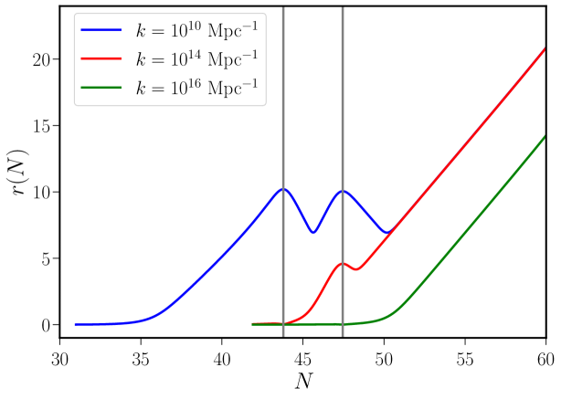
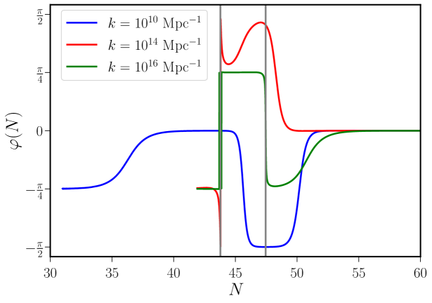
Figure 1: The evolution of the squeezing amplitude $r$ and the squeezing angle $\varphi$ have been plotted (on top and at the bottom, respectively) against the number of e-folds $N$ in the ultra slow roll model of interest. In the figures, we have demarcated the period of ultra slow roll (by gray vertical lines). We have plotted the evolution of the squeezing parameters for modes with the wave numbers $k=(10^{10},10^{14},10^{16})\,\mathrm{Mpc}^{-1}$ (in blue, red and green). While the first and the last of these modes exit the Hubble radius before and after the ultra slow roll phase, the second mode leaves the Hubble radius during the period of ultra slow roll. As we have pointed out, in slow roll inflation, the squeezing parameter $r$ behaves as $r\propto N$ after the modes leave the Hubble radius (in a manner similar to the case of the third wave number, plotted in green). We find that the epoch of ultra slow roll modifies this behavior for modes that leave the Hubble radius immediately prior to or during the ultra slow roll phase (as in the cases for the wave numbers plotted in blue and red). Similarly, in a slow roll scenario, the squeezing parameter $\varphi$ approaches zero monotonically once the modes are on super-Hubble scales. In contrast, as should be evident from the above figure, the epoch of ultra slow roll induces non-trivial behavior. However, note that the parameter $\varphi$ eventually approaches zero for all the wave numbers (barring those that leave the Hubble radius very close to the end of inflation), indicating that the Wigner ellipse orients itself along the $v$-axis towards the end of inflation.

We have plotted the evolution for modes with three different wave numbers that leave the Hubble radius just prior to, during and after the period of ultra slow roll. Note that, despite the non-trivial evolution during the intermediate period, the parameter $\varphi$ eventually approaches zero at adequately late times. We shall soon discuss the impact of the ultra slow roll phase on the squeezing amplitude $r$.

In Fig. 2, we have plotted the scalar power spectra $\mathcal{P}_{{}_{\mathcal{R}}}(k)$ and the squeezing amplitude $r(k)$, obtained numerically, in the above two models for a wide range of wave numbers.

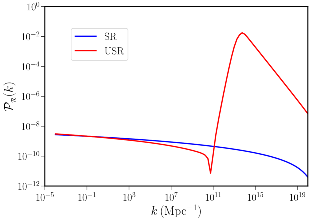
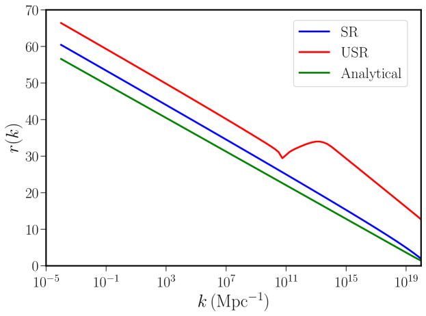
Figure 2: The scalar power spectrum $\mathcal{P}_{{}_{\mathcal{R}}}(k)$ (on top) and the squeezing amplitude $r(k)$ (at the bottom) evaluated towards the end of inflation have been plotted as a function of the wave number for the two single field inflationary models of our interest, viz. the popular model due to Starobinsky that admits only slow roll inflation (SR, in blue) and the other model that leads to a brief period of ultra slow roll (USR, in red). We have evaluated these quantities numerically and, in the case of slow roll inflation, we have also plotted the analytical results for the squeezing amplitude, arrived at in the de Sitter approximation (in green, at the bottom). In slow roll inflation, since $r(N)\propto N$ on super-Hubble scales, the value of the squeezing parameter $r(k)$ associated with a given wave number roughly corresponds to the number of e-folds between the time the mode leaves the Hubble radius and the end of inflation. Note that, in the case of ultra slow roll inflation, the squeezing amplitude corresponding to the small scale modes which exhibit higher power is enhanced to a certain extent when compared to the slow roll case.

As expected, the power spectrum is nearly scale invariant in the slow roll model, while it exhibits a peak with higher power at small scales in the model permitting ultra slow roll inflation. It is the peak with the enhanced power that proves to be responsible for producing a significant number of PBHs in such models Garcia-Bellido:2017mdw ; Ballesteros:2017fsr ; Germani:2017bcs ; Kannike:2017bxn ; Dalianis:2018frf ; Ragavendra:2020sop . Since $r(N)\simeq 0$ on sub-Hubble scales and $r(N)\propto N$ on super-Hubble scales in the slow roll model, towards the end of inflation, we can expect that $r(k)\simeq 60$ for the largest scales, which is clearly reflected in the results plotted in the figure. In fact, using the standard modes in the de Sitter approximation, one can show that, in slow roll,

$$\mathrm{cosh}\,(2\,r)\simeq 1+\frac{k_{\mathrm{e}}^{2}}{2\,k^{2}},\quad\mathrm{tan}\,(2\,\varphi)\simeq-\frac{2\,k}{k_{\mathrm{e}}},$$ (32)

where, as we mentioned, $k_{\mathrm{e}}$ denotes the wave number that leaves the Hubble radius at the end of inflation. In the figure, we have also plotted the above analytical result for $r(k)$. Clearly, the analytical estimate captures the more accurate numerical results fairly well in the slow roll case. Interestingly, in the model involving ultra slow roll inflation, we find that $r(k)$ is boosted to a certain extent over wave numbers which exhibit enhanced scalar power. This can evidently be attributed to the non-trivial evolution of the modes during the epoch of ultra slow roll.

3 Evolution in two field inflationary models

Having discussed the evolution of the quantum state of the curvature perturbations in single field models of inflation, let us now turn to discuss the behavior in two field models. In this section, we shall examine the evolution of the Wigner function, the squeezing parameters and the entanglement entropy describing the curvature perturbation in a model permitting slow roll inflation and a model that leads to enhanced power on small scales, achieved through a turn in the field space. We shall also show that the entanglement entropy for the system of our interest is equivalent to the quantum discord.

3.1 Action and equations governing the background

The two field models of our interest consist of a canonical scalar field $\phi$ and a non-canonical scalar field $\chi$. The system is governed by the following action (see, for instance, Refs. DiMarco:2002eb ; Lalak:2007vi ; Raveendran:2018yyh ; Braglia:2020fms ; Braglia:2020eai ; Palma:2020ejf ):

$$S[\phi,\chi]=\int{\rm d}^{4}x\sqrt{-g}\,\biggl{[}-\frac{1}{2}\,{\partial}_{\mu}\phi\,{\partial}^{\mu}\phi-\,\frac{\mathrm{e}^{2\,b(\phi)}}{2}\,{\partial}_{\mu}\chi\,{\partial}^{\mu}\chi-V(\phi,\chi)\biggr{]},$$ (33)

where, evidently, it is the exponential term involving the function $b(\phi)$ that makes the scalar field $\chi$ non-canonical. The equations of motion governing the homogeneous scalar fields $\phi$ and $\chi$ can be obtained to be

$$\ddot{\phi}+3\,H\,\dot{\phi}+V_{\phi} = b_{\phi}\,\mathrm{e}^{2\,b}\,\dot{\chi}^{2},$$ (34a)

$$\ddot{\chi}+(3\,H+2\,b_{\phi}\,\dot{\phi})\,\dot{\chi}+\mathrm{e}^{-2\,b}\,V_{\chi} = 0,$$ (34b)

where the subscripts $\phi$ and $\chi$ denote differentiation of the potential $V(\phi,\chi)$ and the function $b(\phi)$ with respect to the fields. We should also mention that the Hubble parameter and its time derivative are described by the equations

$$H^{2} = \frac{1}{3\,M_{{}_{\mathrm{Pl}}}^{2}}\,\left(\frac{\dot{\phi}^{2}}{2}+\mathrm{e}^{2\,b}\,\frac{\dot{\chi}^{2}}{2}+V\right),$$ (35)

$$\dot{H} = -\frac{1}{2\,M_{{}_{\mathrm{Pl}}}^{2}}\,\left(\dot{\phi}^{2}+\mathrm{e}^{2\,b}\,\dot{\chi}^{2}\right).$$ (36)

3.2 Action describing the perturbations and quantization

Recall that, in the case of inflation driven by a single scalar field, the perturbations are characterized by the Mukhanov-Sasaki variable associated with the curvature perturbation. In inflationary models involving two fields, it is well known that, apart from the curvature perturbations, isocurvature perturbations also arise (in this context, see the reviews Bassett:2005xm ; Malik:2008im ). Let $v_{\sigma}$ and $v_{s}$ be the Mukhanov-Sasaki variables associated with the curvature and the isocurvature perturbations (or, equivalently, the adiabatic and entropic perturbations), respectively. In order to arrive at the action describing the variables $v_{\sigma}$ and $v_{s}$, it is convenient to introduce the quantities DiMarco:2002eb ; Lalak:2007vi ; Raveendran:2018yyh ; Braglia:2020fms ; Braglia:2020eai ; Palma:2020ejf

$$\mathrm{cos}\,\theta=\frac{\dot{\phi}}{\dot{\sigma}},\quad\mathrm{sin}\,\theta=\mathrm{e}^{b}\,\frac{\dot{\chi}}{\dot{\sigma}},\quad\dot{\sigma}^{2}=\dot{\phi}^{2}+\mathrm{e}^{2\,b}\,\dot{\chi}^{2}$$ (37)

and define the quantities $V_{\sigma}$ and $V_{s}$ to be

$$V_{\sigma}=\mathrm{cos}\,\theta\,V_{\phi}+\mathrm{sin}\,\theta\,{\mathrm{e}}^{-b}\,V_{\chi},\quad V_{s}=-\mathrm{sin}\,\theta\,V_{\phi}+\mathrm{cos}\,\theta\,{\mathrm{e}}^{-b}\,V_{\chi}.$$ (38)

It can be shown that, at the linear order in perturbation theory, the action governing the complete system is given by DiMarco:2002eb ; Lalak:2007vi ; Raveendran:2018yyh ; Braglia:2020fms ; Braglia:2020eai ; Palma:2020ejf

$$S[v_{\sigma}(\eta,\bm{x}),v_{s}(\eta,\bm{x})] = \frac{1}{2}\,\int{\rm d}\eta\int{\rm d}^{3}{\bm{x}}\,\Biggl{\{}v_{\sigma}^{\prime 2}-({\partial}_{i}v_{\sigma})^{2}+v_{s}^{\prime 2}-({\partial}_{i}v_{s})^{2}$$ (39)

$$-\,2\,\frac{z^{\prime}}{z}\,v_{\sigma}^{\prime}\,v_{\sigma}-2\,\frac{a^{\prime}}{a}\,v_{s}^{\prime}\,v_{s}-2\,\xi\,v_{\sigma}^{\prime}\,v_{s}+2\,\xi\,\frac{z^{\prime}}{z}\,v_{\sigma}\,v_{s}$$

$$+\,\left(\frac{z^{\prime}}{z}\right)^{2}\,v_{\sigma}^{2}+\left[\left(\frac{a^{\prime}}{a}\right)^{2}-\mu_{s}^{2}\,a^{2}\right]\,v_{s}^{2}\Biggr{\}},$$

where $z=a\,\dot{\sigma}/H$ and $\xi=-2\,a\,V_{s}/\dot{\sigma}$. Moreover, the quantity $\mu_{s}^{2}$ has been defined to be

$$\mu_{s}^{2}=V_{ss}-\left(\frac{V_{s}}{\dot{\sigma}}\right)^{2}+\mathrm{cos}\,\theta\,\left(1+\mathrm{sin}^{2}\theta\right)\,b_{\phi}\,V_{\sigma}+\mathrm{cos}^{2}\,\theta\,\mathrm{sin}\,\theta\,b_{\phi}\,V_{s}-\dot{\sigma}^{2}\,\left(b_{\phi}^{2}+b_{\phi\phi}\right),$$ (40)

where $V_{ss}$ is given by

$$V_{ss}=\mathrm{sin}^{2}\theta\,V_{\phi\phi}-2\,\mathrm{sin}\,\theta\,\mathrm{cos}\,\theta\,{\mathrm{e}}^{-b}\,V_{\phi\chi}+\mathrm{cos}^{2}\theta\,{\mathrm{e}}^{-2\,b}\,V_{\chi\chi}.$$ (41)

In the spatially flat, FLRW background, we can decompose both the Mukhanov-Sasaki variables $v_{\sigma}$ and $v_{s}$ in terms of the corresponding Fourier modes, say, $v_{\sigma}^{\bm{k}}$ and $v_{s}^{\bm{k}}$, as we had done earlier in the case of the single field models [see Eq. (2)]. Moreover, the fact that $v_{\sigma}(\eta,{\bm{x}})$ and $v_{s}(\eta,{\bm{x}})$ are real quantities leads to the conditions $v_{\sigma}^{-\bm{k}}=v_{\sigma}^{\bm{k}\,\ast}$ and $v_{s}^{-{\bm{k}}}=v_{s}^{\bm{k}\,\ast}$ on the Fourier modes. Further, we can express the Mukhanov-Sasaki variables in Fourier space, viz. $v_{\sigma}^{\bm{k}}$ and $v_{s}^{\bm{k}}$, in terms of their real and imaginary parts as we had done before in Eq. (4). When we do so, we find that the real and the imaginary parts of the variables $v_{\sigma}^{\bm{k}}$ and $v_{s}^{{\bm{k}}}$ are governed by the action Battarra:2013cha

$$S[v_{\sigma}(\eta),v_{s}(\eta)] = \frac{1}{2}\,\int{\rm d}\eta\,\biggl{(}v_{\sigma}^{\prime 2}+v_{s}^{\prime 2}-2\,\frac{z^{\prime}}{z}v_{\sigma}^{\prime}\,v_{\sigma}-2\,\frac{a^{\prime}}{a}\,v_{s}^{\prime}\,v_{s}$$ (42)

$$-\,2\,\xi\,v_{\sigma}^{\prime}\,v_{s}+2\,\xi\,\frac{z^{\prime}}{z}\,v_{\sigma}\,v_{s}-m_{\sigma}^{2}\,v_{\sigma}^{2}-m_{s}^{2}\,v_{s}^{2}\biggr{)},$$

where, for convenience, we have dropped the superscript ${\bm{k}}$, while the quantities $m_{\sigma}^{2}$ and $m_{s}^{2}$ are given by

$$m_{\sigma}^{2}=k^{2}-\frac{z^{\prime 2}}{z^{2}},\quad m_{s}^{2}=k^{2}-\frac{a^{\prime 2}}{a^{2}}+\mu_{s}^{2}\,a^{2}.$$ (43)

From above action, the equations of motion governing the variables $v_{\sigma}$ and $v_{s}$ can be obtained to be

$$v_{\sigma}^{\prime\prime}+\left(k^{2}-\frac{z^{\prime\prime}}{z}\right)\,v_{\sigma} = \frac{1}{z}\,\left(z\,\xi\,v_{s}\right)^{\prime},$$ (44a)

$$v_{s}^{\prime\prime}+\left(k^{2}-\frac{a^{\prime\prime}}{a}+\mu_{s}^{2}\,a^{2}\right)\,v_{s} = -z\,\xi\,\left(\frac{v_{\sigma}}{z}\right)^{\prime}.$$ (44b)

The momenta, say, $p_{\sigma}$ and $p_{s}$, that are conjugate to the variables $v_{\sigma}$ and $v_{s}$ can be determined from the action (42) to be

$$p_{\sigma}=v_{\sigma}^{\prime}-\frac{z^{\prime}}{z}\,v_{\sigma}-\xi\,v_{s},\quad p_{s}=v_{s}^{\prime}-\frac{a^{\prime}}{a}\,v_{s}.$$ (45)

The Hamiltonian, say, $H_{2}$, of the complete system is then given by

$$H_{2} = \frac{1}{2}\,\left(p_{\sigma}+\frac{z^{\prime}}{z}\,v_{\sigma}+\xi\,v_{s}\right)^{2}+\frac{1}{2}\,\left(p_{s}+\frac{a^{\prime}}{a}\,v_{s}\right)^{2}-\xi\,\frac{z^{\prime}}{z}\,v_{\sigma}\,v_{s}$$ (46)

$$+\,\frac{1}{2}\,m_{\sigma}^{2}\,v_{\sigma}^{2}+\frac{1}{2}\,m_{s}^{2}\,v_{s}^{2},$$

and the corresponding, first order, Hamilton’s equations of motion can be obtained to be

$$v_{\sigma}^{\prime} = p_{\sigma}+\frac{z^{\prime}}{z}\,v_{\sigma}+\xi\,v_{s},\quad p_{\sigma}^{\prime}=-\frac{z^{\prime}}{z}\,p_{\sigma}-k^{2}\,v_{\sigma},$$ (47a)

$$v_{s}^{\prime} = p_{s}+\frac{a^{\prime}}{a}\,v_{s},\qquad\qquad p_{s}^{\prime}=-\frac{a^{\prime}}{a}\,p_{s}-\xi\,p_{\sigma}-\left(k^{2}+\mu_{s}^{2}\,a^{2}+\xi^{2}\right)\,v_{s}.\qquad\quad$$ (47b)

Evidently, these equations can be combined to arrive at the corresponding second order equations (44) describing the variables $v_{\sigma}$ and $v_{s}$. Moreover, note that, if we set $v_{s}$ to zero, the above equations reduce to the Hamilton’s equations (9) in the single field case, as required.

If we denote the wave function of the complete system as $\Psi(v_{\sigma},v_{s},\eta)$, then the wave function satisfies the Schrodinger equation Battarra:2013cha

$$i\,\frac{{\partial}\Psi}{{\partial}\eta} = -\frac{1}{2}\,\biggl{[}\frac{{\partial}^{2}\Psi}{{\partial}v_{\sigma}^{2}}+i\,\frac{z^{\prime}}{z}\,\left(\Psi+2\,v_{\sigma}\,\frac{{\partial}\Psi}{{\partial}v_{\sigma}}\right)+\frac{{\partial}^{2}\Psi}{{\partial}v_{s}^{2}}+i\,\frac{a^{\prime}}{a}\,\left(\Psi+2\,v_{s}\,\frac{{\partial}\Psi}{{\partial}v_{s}}\right)$$ (48)

$$+\,2\,i\,\xi\,v_{s}\,\frac{{\partial}\Psi}{{\partial}v_{\sigma}}-k^{2}\,v_{\sigma}^{2}\,\Psi-\left(k^{2}+\xi^{2}+\mu_{s}^{2}\,a^{2}\,\right)\,v_{s}^{2}\,\Psi\biggr{]}.$$

As in the single field case, we shall look for a solution to this Schrodinger equation which has a Gaussian form. Let us start with the following ansatz Battarra:2013cha ; Vachaspati:2018hcu :

$$\Psi(v_{\sigma},v_{s},\eta)={\mathcal{N}}(\eta)\;\mathrm{exp}\left[-\frac{1}{2}\,\Omega_{\sigma\sigma}(\eta)\,v_{\sigma}^{2}-\frac{1}{2}\,\Omega_{ss}(\eta)\,v_{s}^{2}-\Omega_{\sigma s}(\eta)\,v_{\sigma}\,v_{s}\right]$$ (49)

so that the normalization of the wave function leads to the condition

$$|{\mathcal{N}}|=\left[\frac{\Omega_{\sigma\sigma}^{\mathrm{R}}\,\Omega_{ss}^{\mathrm{R}}-\left(\Omega_{\sigma s}^{\mathrm{R}}\right)^{2}}{\pi}\right]^{1/4},$$ (50)

where $(\Omega_{\sigma\sigma}^{\mathrm{R}},\Omega_{ss}^{\mathrm{R}},\Omega_{\sigma s}^{\mathrm{R}})$ denote the real parts of the quantities $(\Omega_{\sigma\sigma},\Omega_{ss},\Omega_{\sigma s})$. Clearly, if we can determine the quantities $(\Omega_{\sigma\sigma},\Omega_{ss},\Omega_{\sigma s})$, we can obtain ${\mathcal{N}}$ modulo an overall phase factor, as in the case of single field models. On substituting the Gaussian ansatz (49) in the Schrodinger equation (48), we find that the quantities $(\Omega_{\sigma\sigma},\Omega_{ss},\Omega_{\sigma s})$ satisfy the differential equations

$$i\,\Omega_{\sigma\sigma}^{\prime} = \left(\Omega_{\sigma\sigma}-i\,\frac{z^{\prime}}{z}\right)^{2}+\Omega_{\sigma s}^{2}-m_{\sigma}^{2},$$ (51a)

$$i\,\Omega_{ss}^{\prime} = \left(\Omega_{ss}-i\,\frac{a^{\prime}}{a}\right)^{2}+\left(\Omega_{\sigma s}-i\,\xi\right)^{2}-m_{s}^{2},$$ (51b)

$$i\,\Omega_{\sigma s}^{\prime} = \left[\Omega_{\sigma\sigma}+\Omega_{ss}-i\left(\frac{z^{\prime}}{z}+\frac{a^{\prime}}{a}\right)\right]\,\Omega_{\sigma s}-i\,\xi\,\Omega_{\sigma\sigma}.$$ (51c)

In the case of two field models, two sets of uncorrelated initial conditions are imposed on the curvature and isocurvature perturbations when the modes are well inside the sub-Hubble radius (for discussions on this point, see, for instance, Refs. Lalak:2007vi ; Raveendran:2018yyh ; Braglia:2020fms ; Braglia:2020eai ). To account for the two sets of initial conditions, let us now write the quantities $(\Omega_{\sigma\sigma},\Omega_{ss},\Omega_{\sigma s})$ as follows Battarra:2013cha :

$$\Omega_{\sigma\sigma} = -i\,\frac{g_{s}^{\ast}\,\pi_{\sigma}^{f\ast}-f_{s}^{\ast}\,\pi_{\sigma}^{g\ast}}{g_{s}^{\ast}\,f_{\sigma}^{\ast}-f_{s}^{\ast}\,g_{\sigma}^{\ast}},$$ (52a)

$$\Omega_{ss} = -i\,\frac{f_{\sigma}^{\ast}\,\pi_{s}^{g\ast}-g_{\sigma}^{\ast}\,\pi_{s}^{f\ast}}{f_{\sigma}^{\ast}\,g_{s}^{\ast}-g_{\sigma}^{\ast}\,f_{s}^{\ast}},$$ (52b)

$$\Omega_{\sigma s} = -i\,\frac{f_{\sigma}^{\ast}\,\pi_{\sigma}^{g\ast}-g_{\sigma}^{\ast}\,\pi_{\sigma}^{f\ast}}{f_{\sigma}^{\ast}\,g_{s}^{\ast}-g_{\sigma}^{\ast}\,f_{s}^{\ast}}=-i\,\frac{g_{s}^{\ast}\,\pi_{s}^{f\ast}-f_{s}^{\ast}\,\pi_{s}^{g\ast}}{g_{s}^{\ast}\,f_{\sigma}^{\ast}-f_{s}^{\ast}\,g_{\sigma}^{\ast}},$$ (52c)

where the quantities $(\pi^{f}_{\sigma},\pi^{f}_{s})$ and $(\pi_{\sigma}^{g},\pi_{s}^{g})$ are defined as

$$\pi^{f}_{\sigma} = f_{\sigma}^{\prime}-\frac{z^{\prime}}{z}\,f_{\sigma}-\xi\,f_{s},\quad\pi^{f}_{s}=f_{s}^{\prime}-\frac{a^{\prime}}{a}\,f_{s},$$ (53a)

$$\pi^{g}_{\sigma} = g_{\sigma}^{\prime}-\frac{z^{\prime}}{z}\,g_{\sigma}-\xi\,g_{s},\quad\pi^{g}_{s}=g_{s}^{\prime}-\frac{a^{\prime}}{a}\,g_{s}.$$ (53b)

If we now substitute the above expressions for $(\Omega_{\sigma\sigma},\Omega_{ss},\Omega_{\sigma s})$ in Eqs. (51), then we find that the quantities $(f_{\sigma},f_{s})$ as well as $(g_{\sigma},g_{s})$ satisfy the differential equations (44) governing the Mukhanov-Sasaki variables $(v_{\sigma},v_{s})$. Clearly, the quantities $(f_{\sigma},f_{s})$ and $(g_{\sigma},g_{s})$ correspond to the solutions to the Mukhanov-Sasaki variables for the two sets of initial conditions, while the quantities $(\pi^{f}_{\sigma},\pi^{f}_{s})$ and $(\pi_{\sigma}^{g},\pi_{s}^{g})$ can be considered as describing momenta that are conjugate to these solutions. As in the case of single field models, the initial conditions can be imposed when the modes are deep inside the Hubble radius, i.e. when $k\gg\sqrt{z^{\prime\prime}/z}$. In such a domain, one finds that the equations of motion governing the variables $(v_{\sigma},v_{s})$ decouple. Hence, the two sets of initial conditions corresponding to the Bunch-Davies vacuum are given by Lalak:2007vi ; Raveendran:2018yyh ; Braglia:2020fms ; Braglia:2020eai

$$f_{\sigma}(\eta_{\mathrm{i}}) = \frac{1}{\sqrt{2\,k}}\,\mathrm{e}^{-i\,k\,\eta_{\mathrm{i}}},\quad\pi_{\sigma}^{f}(\eta_{\mathrm{i}})=-\frac{1}{\sqrt{2\,k}}\,\left[i\,k+\frac{z^{\prime}(\eta_{\mathrm{i}})}{z(\eta_{\mathrm{i}})}\right]\,\mathrm{e}^{-i\,k\,\eta_{\mathrm{i}}},$$

$$f_{s}(\eta_{\mathrm{i}}) = 0,\quad\pi_{s}^{f}(\eta_{\mathrm{i}})=-\xi(\eta_{\mathrm{i}})\,\frac{1}{\sqrt{2\,k}}\,\mathrm{e}^{-i\,k\,\eta_{\mathrm{i}}},$$ (54a)

$$g_{\sigma}(\eta_{\mathrm{i}}) = 0,\quad\pi_{\sigma}^{g}(\eta_{\mathrm{i}})=-\xi(\eta_{\mathrm{i}})\,\frac{1}{\sqrt{2\,k}}\,\mathrm{e}^{-i\,k\,\eta_{\mathrm{i}}},$$

$$g_{s}(\eta_{\mathrm{i}}) = \frac{1}{\sqrt{2\,k}}\,\mathrm{e}^{-i\,k\,\eta_{\mathrm{i}}},\quad\pi_{s}^{g}(\eta_{\mathrm{i}})=-\frac{1}{\sqrt{2\,k}}\,\left[i\,k+\frac{a^{\prime}(\eta_{\mathrm{i}})}{a(\eta_{\mathrm{i}})}\right]\,\mathrm{e}^{-i\,k\,\eta_{\mathrm{i}}}.$$ (54b)

In the two field case, there arise four Wronskians Battarra:2013cha . By choosing the above initial conditions, we have set them to the following canonical values:

$$f_{\sigma}\,\pi_{\sigma}^{f\ast}+f_{s}\,\pi_{s}^{f\ast}-\left(f_{\sigma}\,\pi_{\sigma}^{f\ast}+f_{s}\,\pi_{s}^{f\ast}\right)^{\ast} = i,$$ (55a)

$$g_{\sigma}\,\pi_{\sigma}^{g\ast}+g_{s}\,\pi_{s}^{g\ast}-\left(g_{\sigma}\,\pi_{\sigma}^{g\ast}+g_{s}\,\pi_{s}^{g\ast}\right)^{\ast} = i,$$ (55b)

$$f_{\sigma}\,\pi_{\sigma}^{g\ast}+f_{s}\,\pi_{s}^{g\ast}-\left(g_{\sigma}\,\pi_{\sigma}^{f\ast}+g_{s}\,\pi_{s}^{f\ast}\right) = 0,$$ (55c)

$$f_{\sigma}\,\pi_{\sigma}^{g}+f_{s}\,\pi_{s}^{g}-\left(g_{\sigma}\,\pi_{\sigma}^{f}+g_{s}\,\pi_{s}^{f}\right) = 0.$$ (55d)

Note that, for better numerical accuracy, we shall solve the first order equations (47) to determine the different measures describing the evolution of the quantum state of the system.

3.3 Wigner function and squeezing parameters

Let $x$ and $y$ denote the variables associated with a system with two degrees of freedom. If $p_{x}$ and $p_{y}$ represent the corresponding conjugate momenta, the Wigner function associated with the wave function $\Psi(x,y,t)$ describing the system is defined as (see, for instance, Ref. Hillery:1983ms )

$$W(x,p_{x},y,p_{y},t) = \frac{1}{\pi^{2}}\,\int_{-\infty}^{\infty}dz_{1}\int_{-\infty}^{\infty}dz_{2}\;\Psi(x-z_{1},y-z_{2},t)$$ (56)

$$\times\,\Psi^{\ast}(x+z_{1},y+z_{2},t)\,\mathrm{e}^{2\,i\,(p_{x}\,z_{1}+p_{y}\,z_{2})}.$$

Since the density matrix associated with the wave function $\Psi(x,y,t)$ is given by

$$\rho(x,y,\bar{x},\bar{y},t)=\Psi(x,y,t)\,\Psi^{\ast}(\bar{x},\bar{y},t),$$ (57)

the above Wigner function can be expressed in terms of the density matrix as follows:

$$W(x,p_{x},y,p_{y},t) = \frac{1}{\pi^{2}}\,\int_{-\infty}^{\infty}dz_{1}\int_{-\infty}^{\infty}dz_{2}\;\rho(x-z_{1},y-z_{2},x+z_{1},y+z_{2},t)$$ (58)

$$\times\,\mathrm{e}^{2\,i\,(p_{x}\,z_{1}+p_{y}\,z_{2})}.$$

In fact, such an expression for the Wigner function allows us to extend the definition to even mixed states Hillery:1983ms ; case2008wigner .

In principle, we can evaluate the complete Wigner function associated with the Gaussian wave function $\Psi(v_{\sigma},v_{s},\eta)$, which we had assumed to describe the system of our interest [see Eq. (49)]. However, in this work, we shall focus only on the reduced dynamics associated with the curvature perturbation or, more precisely, the corresponding Mukhanov-Sasaki variable $v_{\sigma}$. Further, in due course, we shall be interested in evaluating the entanglement entropy (or, equivalently, the quantum discord) associated with the variable $v_{\sigma}$. For these reasons, we shall first evaluate the reduced density matrix describing $v_{\sigma}$ and utilize it to arrive at the corresponding Wigner function $W(v_{\sigma},p_{\sigma},\eta)$.

Motivated by the expression (58) for the Wigner function in terms of the density matrix, we can define the reduced Wigner function associated with the variable $v_{\sigma}$ to be Prokopec:2006fc ; Battarra:2013cha

$$W(v_{\sigma},p_{\sigma},\eta)=\frac{1}{\pi}\,\int_{-\infty}^{\infty}dz_{1}\,\rho_{r}(v_{\sigma}-z_{1},v_{\sigma}+z_{1},\eta)\,\mathrm{e}^{2\,i\,p_{\sigma}\,z_{1}},$$ (59)

where the reduced density matrix $\rho_{r}(v_{\sigma},\bar{v}_{\sigma},\eta)$ is given by

$$\rho_{r}(v_{\sigma},\bar{v}_{\sigma},\eta)=\int{\rm d}v_{s}\,\Psi(v_{\sigma},v_{s},\eta)\,\Psi^{\ast}(\bar{v}_{\sigma},v_{s},\eta).$$ (60)

Upon substituting the wave function $\Psi(v_{\sigma},v_{s},\eta)$ from Eq. (49) in this expression and carrying out the integral over $v_{s}$, we find that the reduced density matrix can be written as

$$\rho_{r}(v_{\sigma},\bar{v}_{\sigma},\eta) = \bar{{\mathcal{N}}}\,\mathrm{exp}\biggl{[}-\left(\frac{C_{SS}}{4}+C_{DD}\right)\,\frac{(v_{\sigma}^{2}+\bar{v}_{\sigma}^{2})}{2}$$ (61)

$$-\,i\,C_{SD}\,\frac{(v_{\sigma}^{2}-\bar{v}_{\sigma}^{2})}{2}+\left(C_{DD}-\frac{C_{SS}}{4}\right)\,v_{\sigma}\,\bar{v}_{\sigma}\biggr{]},$$

where $\bar{{\mathcal{N}}}$ is a normalization factor which ensures that the trace of the density matrix is unity. The quantities $(C_{SS},C_{DD},C_{SD})$ are given by

$$C_{SS} = 2\,\Omega_{\sigma\sigma}^{\mathrm{R}}\,\left(1-\frac{(\Omega_{\sigma s}^{\mathrm{R}})^{2}}{\Omega_{\sigma\sigma}^{\mathrm{R}}\,\Omega_{ss}^{\mathrm{R}}}\right),$$ (62a)

$$C_{DD} = \frac{\Omega_{\sigma\sigma}^{\mathrm{R}}}{2}\,\left(1+\frac{(\Omega_{\sigma s}^{\mathrm{I}})^{2}}{\Omega_{\sigma\sigma}^{\mathrm{R}}\,\Omega_{ss}^{\mathrm{R}}}\right),$$ (62b)

$$C_{SD} = \Omega_{\sigma\sigma}^{\mathrm{I}}\,\left(1-\frac{\Omega_{\sigma s}^{\mathrm{I}}\,\Omega_{\sigma s}^{\mathrm{R}}}{\Omega_{\sigma\sigma}^{\mathrm{I}}\,\Omega_{ss}^{\mathrm{R}}}\right),$$ (62c)

where $(\Omega_{\sigma\sigma}^{\mathrm{I}},\Omega_{ss}^{\mathrm{I}},\Omega_{\sigma s}^{\mathrm{I}})$ denote the imaginary parts of the quantities $(\Omega_{\sigma\sigma},\Omega_{ss},\Omega_{\sigma s})$. Upon using the expressions (52) for $(\Omega_{\sigma\sigma},\Omega_{ss},\Omega_{\sigma s})$, we find that the quantities $(C_{SS},C_{DD},C_{SD})$ can be written as

$$C_{SS} = \left(|f_{\sigma}|^{2}+|g_{\sigma}|^{2}\right)^{-1},$$ (63a)

$$C_{DD} = \frac{C_{SS}}{4}\,\left(1+4\,|g_{\sigma}\,\pi_{\sigma}^{f}-f_{\sigma}\,\pi_{\sigma}^{g}|^{2}\right),$$ (63b)

$$C_{SD} = \frac{C_{SS}}{2}\,\left[\left(f_{\sigma}\,\pi^{f\ast}_{\sigma}+g_{\sigma}\,\pi^{g\ast}_{\sigma}\right)+\left(f_{\sigma}\,\pi^{f\ast}_{\sigma}+g_{\sigma}\,\pi^{g\ast}_{\sigma}\right)^{\ast}\right].$$ (63c)

It is convenient to define new variables from the sum and difference of $v_{\sigma}$ and $\bar{v}_{\sigma}$ as Prokopec:2006fc ; Battarra:2013cha

$$v_{S}=\frac{v_{\sigma}+\bar{v}_{\sigma}}{2},\quad v_{D}=v_{\sigma}-\bar{v}_{\sigma}.$$ (64)

Then, the reduced density matrix (61) takes the form

$$\rho_{r}\left(v_{S}+\frac{v_{D}}{2},v_{S}-\frac{v_{D}}{2}\right)=\bar{{\mathcal{N}}}\,\mathrm{exp}\left[-\frac{1}{2}\,\left(C_{SS}\,v_{S}^{2}+C_{DD}\,v_{D}^{2}+2\,i\,C_{SD}\,v_{S}\,v_{D}\right)\right].$$ (65)

The phenomenon of decoherence occurs when the following condition is satisfied schlosshauer2007decoherence ; Prokopec:2006fc ; Battarra:2013cha :

$$\frac{C_{SS}}{C_{DD}}\ll 1.$$ (66)

We shall see later that this condition corresponds to having a large entanglement entropy.

On making use of the expression (61) for the density matrix in the definition (58) of the Wigner function and carrying out the resulting integral, we arrive at

$$W(v_{\sigma},p_{\sigma},\eta)=\frac{\sqrt{C_{SS}}}{2\,\pi\,\sqrt{C_{DD}}}\;\mathrm{exp}\left[-\frac{C_{SS}}{2}\,v_{\sigma}^{2}-\frac{1}{2\,C_{DD}}\,\left(p_{\sigma}+C_{SD}\,v_{\sigma}\right)^{2}\right].$$ (67)

Note that this Wigner function has a structure that is quite similar to that of the Wigner function in the single field case [cf. Eq. (18)]. The behavior of the Wigner function in phase space can be tracked by following the evolution of Wigner ellipse defined by the relation

$$\frac{C_{SS}}{2}\,v_{\sigma}^{2}+\frac{1}{2\,C_{DD}}\,\left(p_{\sigma}+C_{SD}\,v_{\sigma}^{\rm R}\right)^{2}=1.$$ (68)

The reduced Wigner function (67) can again be written in terms of the covariance matrix as we had done in the case of single field models [see Eq. (22)]. However, one finds that, in contrast to the single field case, the area of the Wigner ellipse does not remain constant in two field models (in this context, see App. A). As a result, one requires an extra parameter to describe the covariance matrix. Therefore, instead of Eq. (24), we have cariolaro2015quantum ; Martin:2021znx

$$V\! = \!\frac{(2\,N_{\sigma}+1)}{2}$$

$$\!\!\!\!\times\,\!\!\begin{bmatrix}\cosh\,(2\,r_{\sigma})+\sinh\,(2\,r_{\sigma})\,\cos\,(2\,\varphi_{\sigma})&\sinh\,(2\,r_{\sigma})\,\sin\,(2\,\varphi_{\sigma})\\ \sinh\,(2\,r_{\sigma})\,\sin(2\,\phi_{\sigma})&\cosh\,(2\,r_{\sigma})-\sinh\,(2\,r_{\sigma})\,\cos\,(2\,\varphi_{\sigma})\end{bmatrix}.$$

In other words, when compared to the single field case, the variances are multiplied by an extra factor, leading to

$$\langle\hat{v}_{\sigma}^{2}\rangle = |f_{\sigma}|^{2}+|g_{\sigma}|^{2}$$ (70a)

$$= \frac{(2\,N_{\sigma}+1)}{2\,k}\,\left[\cosh\,(2\,r_{\sigma})+\sinh\,(2\,r_{\sigma})\,\cos\,(2\,\varphi_{\sigma})\right],$$

$$\langle\hat{p}_{\sigma}^{2}\rangle = |\pi_{\sigma}^{f}|^{2}+|\pi_{\sigma}^{g}|^{2}$$ (70b)

$$= \frac{(2\,N_{\sigma}+1)\,k}{2}\,\left[\cosh\,(2\,r_{\sigma})-\sinh\,(2\,r_{\sigma})\,\cos\,(2\,\varphi_{\sigma})\right],\qquad\quad$$

$$\frac{1}{2}\,\langle\hat{v}_{\sigma}\,\hat{p}_{\sigma}+\hat{p}_{\sigma}\,\hat{v}_{\sigma}\rangle = \frac{1}{2}\,\left[\left(f_{\sigma}\,\pi^{f\ast}_{\sigma}+g_{\sigma}\,\pi^{g\ast}_{\sigma}\right)+\left(f_{\sigma}\,\pi^{f\ast}_{\sigma}+g_{\sigma}\,\pi^{g\ast}_{\sigma}\right)^{\ast}\right]$$ (70c)

$$= \frac{(2\,N_{\sigma}+1)}{2}\,\sinh\,(2\,r_{\sigma})\,\sin\,(2\,\varphi_{\sigma}).$$

We should clarify that, again, we have omitted the delta functions for simplicity [in this regard, see the comment following Eq. (26)]. We can invert the above relations to express the squeezing parameters $r_{\sigma}$ and $\varphi_{\sigma}$ as

$$\cosh\,(2\,r_{\sigma}) = \frac{1}{(2\,N_{\sigma}+1)}\,\left[k\,\left(|f_{\sigma}|^{2}+|g_{\sigma}|^{2}\right)+\frac{1}{k}\,\left(|\pi_{\sigma}^{f}|^{2}+|\pi_{\sigma}^{g}|^{2}\right)\right],$$ (71a)

$$\cos\,(2\,\varphi_{\sigma}) = \frac{1}{(2\,N_{\sigma}+1)}\,\frac{1}{\sinh\,(2\,r_{\sigma})}\,\left[k\,\left(|f_{\sigma}|^{2}+|g_{\sigma}|^{2}\right)-\frac{1}{k}\,\left(|\pi_{\sigma}^{f}|^{2}+|\pi_{\sigma}^{g}|^{2}\right)\right].$$

Also, note that the quantity $N_{\sigma}$ is determined through the relation [see Eq. (63)]

$$(2\,N_{\sigma}+1)^{2}=4\,\langle\hat{v}_{\sigma}^{2}\rangle\,\langle\hat{p}_{\sigma}^{2}\rangle-\langle\hat{v}_{\sigma}\,\hat{p}_{\sigma}+\hat{p}_{\sigma}\,\hat{v}_{\sigma}\rangle^{2}=\frac{4\,C_{DD}}{C_{SS}}.$$ (72)

In a subsection that follows, we shall discuss the behavior of the Wigner function and the squeezing parameters in specific two field inflationary models, one that leads to slow roll inflation and another that leads to enhanced power on small scales.

3.4 Entanglement entropy and quantum discord

In contrast to the single field inflationary models, in the two field models, the presence of the additional degree of freedom leads to an entanglement between the two degrees of freedom. As is well known, a good measure of the degree of quantum entanglement in such a bipartite system is the so-called von Neumann entropy of either of the two subsystems, since they are equal schlosshauer2007decoherence . Given the density matrix $\rho$, the von Neumann entropy $\mathcal{S}(\rho)$ is defined as Adesso:2007tx ; horodecki2009quantum

$$\mathcal{S}(\rho)=-\mathrm{Tr.}\left(\rho\,\mathrm{ln}\,\rho\right).$$ (73)

We shall use the von Neumann entropy associated with the reduced density matrix in (61) to quantify the entanglement Prokopec:1992ia ; Prokopec:2006fc ; Battarra:2013cha . But, before we do so, let us understand the relation between the entanglement entropy and the quantum discord in the system of our interest.

Over the past two decades or so, various other measures of correlation have been discovered that are decidedly quantum in nature (in the sense that they should be zero in our classical notion of the world but can be non-zero for systems that have zero entanglement). The most popular of these ideas is the measure of quantum discord (see Refs. zurek2002einselection ; ollivier2001quantum ; henderson2001classical ; for reviews in this context, see Refs. modi2014pedagogical ; bera2017quantum ). As we mentioned, quantum discord can be non-zero even when entanglement is zero. On the other hand, if the quantum discord is zero, then so is the entanglement (for a discussion on how the zero-discord states form a much smaller subset of the separable—zero entanglement—states, see Refs. modi2014pedagogical ; bera2017quantum ). Thus, quantum discord seems to be a better tool than quantum entanglement to look for non-classical correlations in a system.

There are various ways of defining quantum discord bera2017quantum and we shall be using the original measurement-based version, which is what has been used previously in the context of cosmology (see, for instance, Refs. Lim:2014uea ; Martin:2015qta ; Hollowood:2017bil ; Martin:2021znx ). (Note that the quantum discord between two systems depends on which of the two systems is chosen for measurement and hence it is not symmetric. For two systems, say, $\mathbbm{1}$ and $\mathbbm{2}$, choosing $\mathbbm{2}$ for measurements and choosing $\mathbbm{1}$ for measurements will give two different values for quantum discord. But, as we shall see, quantum discord coincides with entanglement entropy when the total system is in a pure state wherein it is symmetric.) Moreover, since we will be dealing with Gaussian states, we shall specialize to Gaussian quantum discord bera2017quantum . In such cases, we have a closed form expression that allows us to calculate quantum discord directly from the covariance matrix adesso2010quantum . In fact, this has been used earlier to calculate quantum discord of cosmological perturbations Lim:2014uea . We shall utilize this expression to determine the quantum discord in the two field inflationary models of our interest.

Even though we have made it a point to stress that quantum discord is separate from entanglement, it turns out that the quantum discord that arises when a system in a pure state is divided into two subsystems is identical to the entanglement entropy (i.e. the von Neumann entropy) bera2017quantum ; datta2008quantum . We shall be evaluating the quantum discord when the pure quantum state of perturbations in the two field inflationary model is divided into curvature and isocurvature perturbations. Thus, it is enough to calculate the entanglement entropy to obtain the discord. Nevertheless, in this subsection, we shall evaluate the complete expression for quantum discord and show that it is indeed equivalent to the entanglement entropy.

We shall now describe how Gaussian quantum discord can be evaluated from the covariance matrix adesso2010quantum . For two degrees of freedom, let $\hat{x}_{1},\hat{p}_{1},\hat{x}_{2},\hat{p}_{2}$ be the two pairs of canonical operators. We arrange them into the vector $\hat{{\textrm{Z}}}=(\hat{x}_{1},\hat{p}_{1},\hat{x}_{2},\hat{p}_{2})$. To connect with the earlier notation (in Ref. adesso2010quantum ), we define a scaled covariance matrix from the covariance matrix in Eq. (23) as

$$\sigma_{ij}=2\,V_{ij}=\langle\hat{{\textrm{Z}}}_{i}\,\hat{{\textrm{Z}}}_{j}+\hat{{\textrm{Z}}}_{j}\,\hat{{\textrm{Z}}}_{i}\rangle.$$ (74)

Decomposing this $(4\times 4)$ matrix in terms of $(2\times 2)$ sub-blocks, we write

$$\bm{\sigma}=\begin{bmatrix}\bm{\alpha}&\bm{\gamma}\\ \bm{\gamma}^{T}&\bm{\beta}\end{bmatrix},$$ (75)

where $\bm{\alpha}$, $\bm{\beta}$ and $\bm{\gamma}$ are $(2\times 2)$ matrices. Local symplectic operations [symplectic operations that act on the subspaces $(\hat{x}_{1},\hat{p}_{1})$ and $(\hat{x}_{2},\hat{p}_{2})$ without mixing them] will have the four independent invariants Serafini:2003ke ; Simon:1999lfr , viz.

$$A=\mathrm{det.}\leavevmode\nobreak\ \bm{\alpha},\quad B=\mathrm{det.}\leavevmode\nobreak\ \bm{\beta},\quad C=\mathrm{det.}\leavevmode\nobreak\ \bm{\gamma},\quad D=\mathrm{det.}\leavevmode\nobreak\ \sigma.$$ (76)

The entanglement entropy for the $(\hat{x}_{2},\hat{p}_{2})$ subsystem, say, $\mathcal{S}_{2}(\sigma_{\mathbbm{12}})$, may then be directly calculated to be Serafini:2003ke

$$\mathcal{S}_{2}(\sigma_{\mathbbm{12}})=F(\sqrt{B}),$$ (77)

with the function $F(x)$ being given by

$$F(x)=\left(\frac{x+1}{2}\right)\,\ln\left(\frac{x+1}{2}\right)-\left(\frac{x-1}{2}\right)\ln\left(\frac{x-1}{2}\right).$$ (78)

As is well-known, the entanglement entropy is the same for both subsystems of a bipartite pure state weedbrook2012gaussian . So, this is also the entanglement entropy of the $(\hat{x}_{1},\hat{p}_{1})$ system.

For the wave function (49) in the two field models of our interest, we can evaluate the elements of the covariance matrix using, say, Mathematica. We obtain the sub-determinants (76) to be

$$A = B=\frac{\left(\Omega^{\mathrm{I}}_{\sigma s}\right)^{2}+\Omega^{\mathrm{R}}_{\sigma\sigma}\,\Omega^{\mathrm{R}}_{ss}}{\Omega^{\mathrm{R}}_{\sigma\sigma}\,\Omega^{\mathrm{R}}_{ss}-\left(\Omega^{\mathrm{R}}_{\sigma s}\right)^{2}},$$ (79a)

$$\ C = -\frac{\left(\Omega^{\mathrm{I}}_{\sigma s}\right)^{2}+\left(\Omega^{\mathrm{R}}_{\sigma s}\right)^{2}}{\Omega^{\mathrm{R}}_{\sigma\sigma}\,\Omega^{\mathrm{R}}_{ss}-\left(\Omega^{\mathrm{R}}_{\sigma s}\right)^{2}},$$ (79b)

$$D = 1.$$ (79c)

We find that the sub-determinants $A$ and $B$ have a simple expression in terms of the coefficients (62) that describe the reduced density matrix (61) associated with the curvature perturbation. It can be established that the sub-determinants have the following simple form:

$$A=B=\frac{4\,C_{DD}}{C_{SS}}.$$ (80)

Therefore, the entanglement entropy can be expressed as

$$\mathcal{S}_{2}(\sigma_{\mathbbm{12}})=F\left(\sqrt{\frac{4\,C_{DD}}{C_{SS}}}\right),$$ (81)

with the function $F(x)$ defined in Eq. (78).

The function $F(x)$ is monotonic when $x\geq 1$ (which is when the function is real). From Eq. (79a), it should be clear that $B$ is greater than or equal to one. Thus, $B$, or equivalently $4\,C_{DD}/C_{SS}$, is by itself a good measure of the entanglement entropy. In fact, it is nothing but the quantity $(2\,N_{\sigma}+1)^{2}$ [see Eq. (72)], and hence is related to the area of the Wigner ellipse [see Eq. (100)]. Therefore, the area of the Wigner ellipse increases as the entropy increases. As we had pointed out earlier following Eq. (66), the growth in entanglement entropy signifies the process of decoherence. Consequently, the growth in the area of the Wigner ellipse beyond the value for a pure state (wherein $N_{\sigma}=0$) is a measure of the decoherence of the system (for related discussions, see Refs. Koksma:2010zi ; Martin:2021znx ).

The symplectic eigenvalues of the covariance matrix $\bm{\sigma}$ can be written in terms of the sub-determinants adesso2010quantum . Defining $\Delta$ as

$$\Delta=A+B+2\,C,$$ (82)

we have the following expression for the symplectic eigen values $\nu_{+}$ and $\nu_{-}$:

$$\nu_{\pm}^{2}=\frac{1}{2}\left(\Delta\pm\sqrt{\Delta^{2}-4D}\right)\leavevmode\nobreak\ .$$ (83)

The relevant point for us is that quantum discord can be written in terms of the above invariants adesso2010quantum . The quantum discord when the measurements are made on the subsystem represented by $(\hat{x}_{2},\hat{p}_{2})$ can be expressed in a closed form as follows:

$$\mathcal{D}(\sigma_{\mathbbm{12}})=F(\sqrt{B})+F(\sqrt{E_{\min}})-\left[F(\nu_{-})+F(\nu_{+})\right],$$ (84)

with the function $F$ defined in Eq. (78) and

$$E_{\min}=\left\{\begin{array}[]{c}\frac{2\,C^{2}+(-1+B)\,(-A+D)+2\,|C|\,\sqrt{C^{2}+(-1+B)\,(-A+D)}}{(-1+B)^{2}}\\ \hbox{when}\;\;(D-A\,B)^{2}\leq(1+B)\,(A+D)\,C^{2},\\ \frac{{A\,B-C^{2}+D-\sqrt{C^{4}+(-A\,B+D)^{2}-2\,C^{2}\,(AB+D)}}}{{2\,B}}\\ \hbox{otherwise}.\end{array}\right.$$ (89)

When the full system is in a pure state, quantum discord is supposed to coincide with the entanglement entropy (i.e. the von Neumann entropy in our case), and we should obtain datta2008quantum

$$\mathcal{D}(\sigma_{\mathbbm{12}})=F(\sqrt{B}),$$ (90)

i.e. the entanglement entropy for the $(\hat{x}_{2},\hat{p}_{2})$ subsystem, the system that is measured. We have explicitly checked the result in Eq. (90) for the general two field wave function in Eq. (49). Upon using Eq. (83), we obtain the symplectic eigen values to be $\nu_{+}=\nu_{-}=1$. Moreover, $E_{\min}$ from Eq. (89) also turns out to be unity. We should mention that, in evaluating the above, we have set $|C|$ to be $-C$, since $C$ is negative [see Eq. (79b)]. (The numerator is obviously negative. The denominator needs to be positive for the normalizability of the wave function.) On substituting these values into Eq. (84), and using $F(1)=0$ as can be proved using a limiting process, we obtain the equality in Eq. (90), which implies that the quantum discord coincides with the entanglement entropy.

3.5 Behavior in specific two field inflationary models

In this section, we shall evaluate the Wigner function, squeezing parameters and entanglement entropy in specific two field models of inflation described by the action (33). We shall consider a potential $V(\phi,\chi)$ that is separable and is given by

$$V(\phi,\chi)=\frac{m^{2}}{2}\,(\phi^{2}+\chi^{2}).$$ (91)

Therefore, the interaction between the two fields $\phi$ and $\chi$ arises only due to the function $b(\phi)$. We shall work with the following form for the function $b(\phi)$:

$$b(\phi)=\frac{b_{1}}{2}\,\biggl{\{}1+\tanh\,\left[\alpha\,(\phi-\phi_{0})\right]\biggr{\}}.$$ (92)

We shall first consider a slow roll scenario wherein $b_{1}=0$. Since $b_{1}=0$, $b(\phi)$ vanishes, and the field $\chi$ reduces to that of a canonical scalar field. Also, there arises no interaction between the two fields. To ensure COBE normalization on large scales, we shall set $m=9\times 10^{-6}\,M_{{}_{\mathrm{Pl}}}$. We choose the initial values of the fields and their velocities to be $\phi_{\mathrm{i}}=\chi_{\mathrm{i}}=11.5\,M_{{}_{\mathrm{Pl}}}$ and $\dot{\phi}_{\mathrm{i}}=\dot{\chi}_{\mathrm{i}}=-3.68\times 10^{-6}\,M_{{}_{\mathrm{Pl}}}^{2}$. We find that, under these conditions, inflation lasts for about $66$ e-folds. As the potential $V(\phi,\chi)$ has the same form along the two field directions, for the above choice of initial conditions, both the fields evolve in the same manner. In other words, the evolution of the background is radial in field space and, hence, the behavior of the perturbations effectively reduces to the behavior in a single field model.

For achieving the scenario which leads to enhanced power on small scales, we shall set $m=1.03\times 10^{-5}\,M_{{}_{\mathrm{Pl}}}$, $b_{1}=15$, $\alpha=10\,M_{{}_{\mathrm{Pl}}}^{-1}$ and $\phi_{0}=6\,M_{{}_{\mathrm{Pl}}}$. We shall choose the initial conditions to be $(\phi_{\mathrm{i}},\chi_{\mathrm{i}})=(13\,M_{{}_{\mathrm{Pl}}},6\,M_{{}_{\mathrm{Pl}}})$ and $(\dot{\phi}_{\mathrm{i}},\dot{\chi}_{\mathrm{i}})=(-5.44\times 10^{-6}\,M_{{}_{\mathrm{Pl}}}^{2},0)$. For such values and conditions, we find that inflation proceeds for about $66$ e-folds before it is terminated. The non-zero value for $b_{1}$ induces an interaction between the two fields. In Fig. 3, we have plotted the evolution of the two fields $\phi$ and $\chi$ as a function of e-folds.

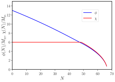
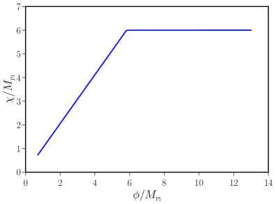
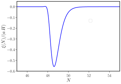
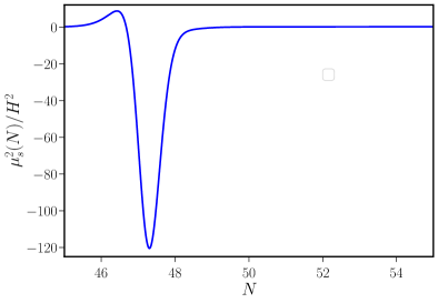
Figure 3: The evolution of the fields $\phi$ (in blue) and $\chi$ (in red) in the two field inflationary model of our interest with a non-zero $b_{1}$ has been plotted against the number of e-folds (on top left) as well as in field space (on top right). We have also plotted interaction strength $\xi$ between the curvature and the isocurvature perturbations (on bottom left) and the effective mass squared $\mu_{s}^{2}$ of the isocurvature perturbations (on bottom right). It should be clear from these figures that $\xi$ increases (during $47\lesssim N\lesssim 50$) and $\mu_{s}^{2}$ becomes negative (during $46\lesssim N\lesssim 48$) as the field turns in space. These two effects combine to result in enhanced power over wave numbers which leave the Hubble radius during this period.

We have also illustrated their evolution in field space. Moreover, in the figure, we have plotted the quantity $\xi$ which characterizes the strength of the interaction between the curvature and the isocurvature perturbations [see Eqs. (44)] as well as the effective mass squared of the isocurvature perturbations $\mu_{s}^{2}$ [see Eq. (40)]. We find that the initial stage of inflation is driven by the field $\phi$, whereas the latter stage is driven by both the fields $\phi$ and $\chi$. The form of the function $b(\phi)$ [see Eq. (92)] induces a turning in the field space as the field $\phi$ approaches $\phi_{0}$. The turn in the field space briefly increases the interaction strength $\xi$ (during the e-folds $47<N<50$) between the curvature and the isocurvature perturbations. In the course of this turning (in fact, during $46<N<48$), the quantity $\mu_{s}^{2}$ becomes negative creating a temporary tachyonic instability. As we shall soon illustrate, the interaction between the curvature and the isocurvature perturbations, coupled with the tachyonic instability, leads to enhanced power on small scales.

Before we proceed, it is important that we clarify a couple of points concerning our choice (91) for the potential $V(\phi,\chi)$ and the functional form (92) of $b(\phi)$. Recall that, in the single field case, the potentials have to be suitably designed to achieve the desired background dynamics and enhanced power on small scales. In contrast, in two field models, we have worked with simple potentials and it is the form of the function $b(\phi)$ that is responsible for the non-trivial background dynamics. While the specific form of $b(\phi)$ that we have worked with [as given by Eq. (92)] seems fine tuned, one can work with simpler forms of $b(\phi)$ and potentials with an additional parameter to achieve similar scalar power spectra. It is the richer dynamics of the two field models, specifically the presence of the non-canonical kinetic term involving $b(\phi)$ and its non-trivial effects on the evolution of the perturbations, that permits such a possibility (in this context, see, for instance, Refs. Braglia:2020eai ; Braglia:2020fms ).

In Fig. 4, we have plotted the evolution of the squeezing amplitude $r_{\sigma}$ associated with the curvature perturbation and the associated squeezing angle $\varphi_{\sigma}$, as a function of e-folds in the scenario which leads to enhanced power on small scales.

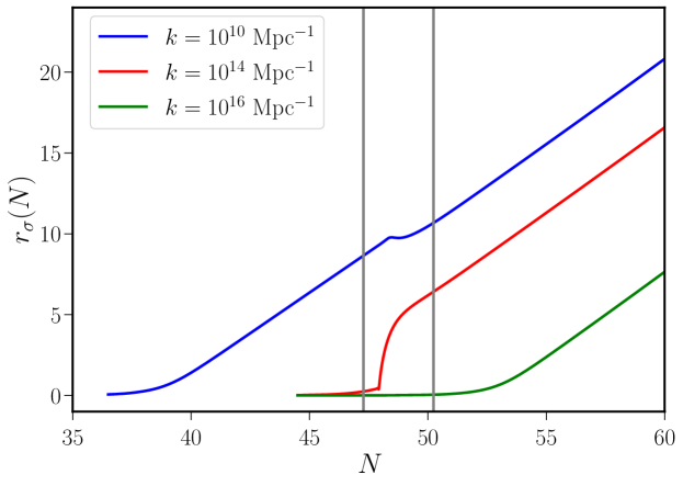
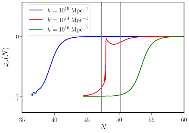
Figure 4: The evolution of the squeezing amplitude $r_{\sigma}$ associated with the curvature perturbation and the corresponding squeezing angle $\varphi_{\sigma}$ has been plotted as a function of e-folds (on top and at the bottom, respectively) in the two field inflationary model which leads to enhanced power on small scales. We have plotted the evolution of the squeezing parameters for modes with the wave numbers $k=(10^{10},10^{14},10^{16})\,\mathrm{Mpc}^{-1}$ (in blue, red and green). We have also demarcated the period when the turning in field space occurs (by gray vertical lines). It should be clear that, during this period, both the squeezing parameters exhibit non-trivial behavior. We find that, as in the single field case, at late times, while $r_{\sigma}(N)\propto N$, $\varphi_{\sigma}$ approaches zero.

We have plotted the squeezing parameters for three different wave numbers which leave the Hubble radius around the time when the turning in the field space occurs. It is clear from the figure that the turning in field space induces non-trivial evolution of the squeezing parameters. However, at adequately late times, after the turn is complete and when the modes are on super-Hubble scales, while $r_{\sigma}\propto N$, $\varphi_{\sigma}$ tends to zero as in the single field case.

In two field inflationary models, the power spectrum of the curvature perturbations is defined as in Eq. (28), with $\hat{v}$ replaced by $\hat{v}_{\sigma}$. Upon using the expression (70a) for $\langle\hat{v}_{\sigma}^{2}\rangle$, we obtain that

$$\mathcal{P}_{{}_{\mathcal{R}}}(k) = \frac{k^{2}}{4\,\pi^{2}\,z^{2}}\,(2\,N_{\sigma}+1)\,\left[\cosh\,(2\,r_{\sigma})+\sinh\,(2\,r_{\sigma})\,\cos\,(2\,\varphi_{\sigma})\right]$$ (93)

$$= \frac{k^{3}}{2\,\pi^{2}\,z^{2}}\,\left(|f_{\sigma}|^{2}+|g_{\sigma}|^{2}\right),$$

where $N_{\sigma}$ is determined by the relation (72). In Fig. 5, we have plotted the power spectrum of the curvature perturbation and the squeezing amplitude in the slow roll scenario as well as the scenario involving a turn in field space.

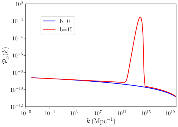
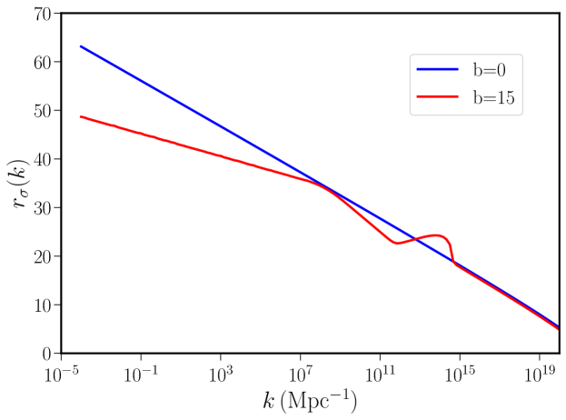
Figure 5: The power spectrum of the curvature perturbations $\mathcal{P}_{{}_{\mathcal{R}}}(k)$ (on top) and the squeezing amplitude $r_{\sigma}(k)$ (at the bottom), evaluated towards the end of inflation, have been plotted as a function of wave numbers in both the two field inflationary models we have considered, viz. the one that permits only slow roll inflation and another that leads to a turn in the field space. While the spectrum of curvature perturbations is nearly scale invariant in the slow roll model, the scenario involving the turn in field space leads to a sharp peak in the spectrum. The non-trivial evolution that is responsible for the peak in the power spectrum also modifies the shape of $r_{\sigma}(k)$, which too exhibits a small peak around the wave number at which the scalar power spectrum $\mathcal{P}_{{}_{\mathcal{R}}}(k)$ contains the peak.

We have plotted these quantities for a wide range of wave numbers. Clearly, while we obtain a nearly scale invariant spectrum in the slow roll case, the scenario involving the turn in the field space leads to enhanced amplitude on smaller scales with a peak in the power spectrum. Also, as in the single field models, at the end of inflation, $r_{\sigma}$ is roughly determined by the amount of time the modes spend on super-Hubble scales. We find that the scenario involving the turn in field space leads to slightly lower or higher values of $r_{\sigma}$ for modes that leave the Hubble radius during the turn. Interestingly, the quantity $r_{\sigma}(k)$ exhibits a peak around the same location as the spectrum of curvature perturbations $\mathcal{P}_{{}_{\mathcal{R}}}(k)$.

Let us now turn to understand the behavior of the entanglement entropy, which is an additional measure describing the evolution of the curvature perturbations in two field models. It is easy to establish that, in the slow roll scenario, the entanglement entropy $\mathcal{S}(k)$ associated with the curvature perturbations vanishes identically. This is because of the fact that, since the dynamics of the two fields are the same (due to the choice of the potential and the initial conditions), the system effectively behaves as in the case of a single scalar field. In Fig. 6, we have plotted the entanglement entropy $\mathcal{S}(k)$ in the non-trivial scenario involving the turn in field space.

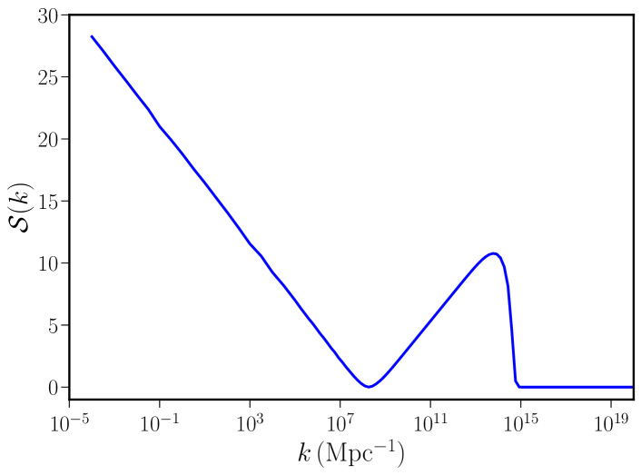
Figure 6: The entanglement entropy—or, equivalently, the quantum discord—$\mathcal{S}(k)$ associated with the curvature perturbations in the two field model has been plotted for the scenario involving a turn in the field space. Note that the entanglement entropy is higher over large scales and is lower over small scales. We find that the modes that leave the Hubble radius during the turning in field space exhibit a higher level of entanglement entropy, with the peak corresponding to the peak in the spectrum of curvature perturbations.

We find that the entanglement entropy is higher over large scales when compared to smaller scales. Interestingly, in a manner similar to the behavior of the squeezing amplitude $r_{\sigma}(k)$, we find that the entanglement entropy $\mathcal{S}(k)$ also exhibits a peak around the same location as the spectrum of curvature perturbations $\mathcal{P}_{{}_{\mathcal{R}}}(k)$.

4 Discussion

In this work, we have examined the evolution of the quantum state of the curvature perturbations in single and two field models of inflation. In the case of single field models, we have used mathematical measures such as the behavior of the Wigner function and the squeezing parameters to understand the manner in which the quantum state of the system evolves. In the case of two field models, apart from the measures mentioned above, we have also examined the behavior of the entanglement entropy (arrived at by integrating the degrees of freedom associated with the isocurvature perturbations) or, equivalently, quantum discord. We have compared the behavior of these measures in slow roll inflation with the corresponding behavior in models that lead to departures from slow roll and enhanced power on small scales. We find that the departures from slow roll inflation can modify or boost these measures to only to a limited extent.

In the case of the single field models, we had partitioned the system into real and imaginary parts of the Fourier modes of the Mukhanov-Sasaki variable. Since these quantities were decoupled, no entanglement entropy or quantum discord arose in this case. On the other hand, if we work in terms of the Fourier modes themselves, entanglement and discord can arise if we partition the system into ${\bm{k}}$ and $-{\bm{k}}$ sectors Martin:2015qta . (We have, in fact, checked that, upon using the wave function provided in Ref. Martin:2019wta in Eq. (90), we can arrive at expression for quantum discord obtained in Ref. Martin:2015qta .) Even in the case of two field models, one may partition the system into ${\bm{k}}$ and $-{\bm{k}}$ sectors and study the resulting entanglement entropy and quantum discord. We shall leave these avenues for future work.

Another topic to be explored is decoherence due to interactions with an environment. There are very many ways in which such an environment may be constructed (in this context, see, for example, Ref. Kiefer:2008ku ). One may consider interactions with other fields. Even otherwise, the full non-linear theory will have interactions between different modes and between the scalar, vector and tensor sectors of the cosmological perturbations. One could also consider interaction between perturbations in different spatial regions, for example the regions inside and outside the Hubble radius. Even the case of two scalar fields, as we have considered, has been claimed to be sufficient to provide decoherence in certain cases Prokopec:2006fc ; Battarra:2013cha . We observe a similar dynamics in our model, and we plan to pursue the topic of decoherence in more detail in a future publication.

Data availability

Data sharing is not applicable to this article as no data sets were generated or analyzed during the current study.

Appendices

Appendix A Geometry of the Wigner ellipse

For a Gaussian Wigner function of the form

$$W(x,p)\propto\mathrm{exp}\left[-\left({\mathcal{A}}\,x^{2}+{\mathcal{B}}\,x\,y+{\mathcal{C}}\,y^{2}\right)\right],$$ (94)

the Wigner ellipse can be defined as the contour described by the quadratic equation

$${\mathcal{A}}\,x^{2}+{\mathcal{B}}\,x\,y+{\mathcal{C}}\,y^{2}=1.$$ (95)

The geometry of an ellipse can be described by specifying the semi-major axis $\bar{a}$, the semi-minor axis $\bar{b}$ and the inclination angle $\delta$, which we shall take to be the angle between the $x$-axis and the major axis, measured anticlockwise from the $x$-axis. While the semi-major and semi-minor axes of the ellipse (95) are given by kendig2005conics

$$\bar{a}^{2}=\frac{2}{{\mathcal{A}}+{\mathcal{C}}-\sqrt{({\mathcal{A}}-{\mathcal{C}})^{2}+{\mathcal{B}}^{2}}},\quad\bar{b}^{2}=\frac{2}{{\mathcal{A}}+{\mathcal{C}}+\sqrt{({\mathcal{A}}-{\mathcal{C}})^{2}+{\mathcal{B}}^{2}}},$$ (96)

the angle $\delta$ is determined by the equations

$$\sin\,(2\,\delta)=\frac{-{\mathcal{B}}}{\sqrt{({\mathcal{A}}-{\mathcal{C}})^{2}+{\mathcal{B}}^{2}}},\quad\cos\,(2\,\delta)=\frac{C-A}{\sqrt{({\mathcal{A}}-{\mathcal{C}})^{2}+{\mathcal{B}}^{2}}}.$$ (97)

We should stress that both these equations are needed to specify the angle $\delta$ in the right quadrant. We take the angle $\delta$ to lie in the range $(-\pi/2,\pi/2]$.

Recall that the Wigner ellipse can be expressed in terms of the covariance matrix $V$ as follows [see Eqs. (21), (22) and (23)]

$$\frac{{\textrm{Z}}^{T}\,V^{-1}\,{\textrm{Z}}}{2}=\frac{V_{22}\,\tilde{v}^{2}-2\,V_{12}\,\tilde{v}\,\tilde{p}+V_{11}\,\tilde{p}^{2}}{2\leavevmode\nobreak\ \textrm{det}\leavevmode\nobreak\ V}=1.$$ (98)

We can apply the formulae (96) and (97) to such a Wigner ellipse, with the general covariance matrix for a mixed Gaussian state given in Eq. (3.3). When we do so, we see that the squeezing amplitude $r_{\sigma}$ is related to the ratio between the minor and major axes and the squeezing angle $\varphi_{\sigma}$ is just the inclination angle $\delta$ between the $\tilde{v}$-axis and the major axis of the ellipse. In other words, we obtain that

$$\frac{\bar{b}^{2}}{\bar{a}^{2}}=\mathrm{e}^{-4\,r_{\sigma}},\quad\delta=\varphi_{\sigma}.$$ (99)

We find that the additional parameter $N_{\sigma}$ we had encountered in the two field case [see Eq. (3.3)] is related to the area of the ellipse by the formula

$$\mathrm{Area}=\pi\,\bar{a}\,\bar{b}=2\,\pi\,\left(2\,N_{\sigma}+1\right).$$ (100)

Note that, in the case of single field models, since $N_{\sigma}=0$, the area of the Wigner ellipse does not change.

Appendix B Conventions of the squeezing parameters

We should point out that, for the squeezing parameters, we have followed the convention adopted earlier in some of the literature (for instance, in Ref. Polarski:1995jg ). Let us consider the case of single field inflationary models. The convention is most transparent in the following parametrization of the Bogoliubov coefficients:

$${\tilde{\alpha}}=\mathrm{e}^{-i\,\vartheta}\,\cosh r,\quad{\tilde{\beta}}=\mathrm{e}^{i\,(2\,\varphi+\vartheta)}\,\sinh r,$$ (101)

with the quantity $r$ assumed to be positive. However, since we have not introduced the Bogoliubov coefficients in this work, we shall explain our convention in terms of variances.

From the discussion in App. A, it should be clear that the quantity $\mathrm{e}^{-4\,r}$ corresponds to the ratio between the minor and the major axes of the Wigner ellipse, while $\varphi$ corresponds to the angle of the major axis of the ellipse with respect to the $\tilde{v}$-axis. Note that the parameter $\vartheta$ does not appear in the covariance matrix (24). One requires only one angle to specify the orientation of the Wigner ellipse, and this orientation may be reached by many different combinations of squeezing and rotation (in this context, see Ref. cariolaro2015quantum ). In the literature on cosmology, the evolution from the vacuum state is usually parametrized as a rotation followed by a squeezing Martin:2015qta . In this case, the rotation operator acting on the initial vacuum state leaves it invariant and only the squeezing parameters appear in the final state.

As we have discussed earlier, in most inflationary scenarios, at late times, $\varphi\to 0$ for a wide range of modes. This implies that, towards the end of inflation, the major axis of the Wigner ellipse will lie along the $\tilde{v}$-axis. In such a limit, the variances are given by

$$\langle\hat{v}^{2}\rangle=\frac{\mathrm{e}^{2\,r}}{2\,k},\quad\langle\hat{p}^{2}\rangle=\frac{k}{2}\,\mathrm{e}^{-2r}.$$ (102)

As the squeezing amplitude $r$ increases on super-Hubble scales, the variance in momentum becomes very small, whereas the variance in position becomes very large. In other words, at late times, the Wigner ellipse is highly squeezed along the $\tilde{v}$-direction and lies on the $\tilde{v}$-axis.

We should mention that our convention matches with that of Ref. Grishchuk:1993ds (except for a change in sign of $\vartheta$, which anyway does not appear in our covariance matrix), but differs from the convention used in Refs. Martin:2015qta ; Martin:2021znx where the squeezing angle $\varphi$ is measured from the $\tilde{p}$-axis.

References

- \bibcommenthead
- (1) Adam, R., et al.: Planck 2015 results. I. Overview of products and scientific results. Astron. Astrophys. 594, 1 (2016) arXiv:1502.01582 [astro-ph.CO]. https://doi.org/10.1051/0004-6361/201527101
- (2) Aghanim, N., et al.: Planck 2018 results. I. Overview and the cosmological legacy of Planck. Astron. Astrophys. 641, 1 (2020) arXiv:1807.06205 [astro-ph.CO]. https://doi.org/10.1051/0004-6361/201833880
- (3) Ade, P.A.R., et al.: Bicep/KeckXV: The Bicep3 Cosmic Microwave Background Polarimeter and the First Three-year Data Set. Astrophys. J. 927(1), 77 (2022) arXiv:2110.00482 [astro-ph.IM]. https://doi.org/10.3847/1538-4357/ac4886
- (4) Mukhanov, V.F., Feldman, H.A., Brandenberger, R.H.: Theory of cosmological perturbations. Part 1. Classical perturbations. Part 2. Quantum theory of perturbations. Part 3. Extensions. Phys. Rept. 215, 203–333 (1992). https://doi.org/10.1016/0370-1573(92)90044-Z
- (5) Martin, J.: Inflation and precision cosmology. Braz. J. Phys. 34, 1307–1321 (2004) arXiv:astro-ph/0312492. https://doi.org/10.1590/S0103-97332004000700005
- (6) Martin, J.: Inflationary cosmological perturbations of quantum-mechanical origin. Lect. Notes Phys. 669, 199–244 (2005) arXiv:hep-th/0406011. https://doi.org/10.1007/11377306_7
- (7) Bassett, B.A., Tsujikawa, S., Wands, D.: Inflation dynamics and reheating. Rev. Mod. Phys. 78, 537–589 (2006) arXiv:astro-ph/0507632. https://doi.org/10.1103/RevModPhys.78.537
- (8) Sriramkumar, L.: An introduction to inflation and cosmological perturbation theory (2009) arXiv:0904.4584 [astro-ph.CO]
- (9) Baumann, D., Peiris, H.V.: Cosmological Inflation: Theory and Observations. Adv. Sci. Lett. 2, 105–120 (2009) arXiv:0810.3022 [astro-ph]. https://doi.org/10.1166/asl.2009.1019
- (10) Baumann, D.: Inflation. In: Theoretical Advanced Study Institute in Elementary Particle Physics: Physics of the Large and the Small, pp. 523–686 (2011). https://doi.org/10.1142/9789814327183_0010
- (11) Sriramkumar, L.: In: Sriramkumar, L., Seshadri, T.R. (eds.) On the generation and evolution of perturbations during inflation and reheating, pp. 207–249 (2012). https://doi.org/10.1142/9789814322072_0008
- (12) Linde, A.: Inflationary cosmology after planck 2013. In: 100e Ecole d’Ete de Physique: Post-Planck Cosmology, pp. 231–316 (2015). https://doi.org/10.1093/acprof:oso/9780198728856.003.0006
- (13) Martin, J.: The Observational Status of Cosmic Inflation after Planck. Astrophys. Space Sci. Proc. 45, 41–134 (2016) arXiv:1502.05733 [astro-ph.CO]. https://doi.org/10.1007/978-3-319-44769-8_2
- (14) Albrecht, A., Ferreira, P., Joyce, M., Prokopec, T.: Inflation and squeezed quantum states. Phys. Rev. D50, 4807–4820 (1994) arXiv:astro-ph/9303001 [astro-ph]. https://doi.org/%****␣qtc_2_field-Nov-2020-sp.bbl␣Line␣250␣****10.1103/PhysRevD.50.4807
- (15) Polarski, D., Starobinsky, A.A.: Semiclassicality and decoherence of cosmological perturbations. Class. Quant. Grav. 13, 377–392 (1996) arXiv:gr-qc/9504030 [gr-qc]. https://doi.org/10.1088/0264-9381/13/3/006
- (16) Kiefer, C., Polarski, D., Starobinsky, A.A.: Quantum to classical transition for fluctuations in the early universe. Int. J. Mod. Phys. D7, 455–462 (1998) arXiv:gr-qc/9802003 [gr-qc]. https://doi.org/10.1142/S0218271898000292
- (17) Kiefer, C., Polarski, D.: Emergence of classicality for primordial fluctuations: Concepts and analogies. Annalen Phys. 7, 137–158 (1998) arXiv:gr-qc/9805014. https://doi.org/%****␣qtc_2_field-Nov-2020-sp.bbl␣Line␣300␣****10.1002/andp.2090070302
- (18) Kiefer, C., Lohmar, I., Polarski, D., Starobinsky, A.A.: Pointer states for primordial fluctuations in inflationary cosmology. Class. Quant. Grav. 24, 1699–1718 (2007) arXiv:astro-ph/0610700 [astro-ph]. https://doi.org/10.1088/0264-9381/24/7/002
- (19) Martin, J.: Inflationary perturbations: The Cosmological Schwinger effect. Lect. Notes Phys. 738, 193–241 (2008) arXiv:0704.3540 [hep-th]. https://doi.org/10.1007/978-3-540-74353-8_6
- (20) Kiefer, C., Polarski, D.: Why do cosmological perturbations look classical to us? Adv. Sci. Lett. 2, 164–173 (2009) arXiv:0810.0087 [astro-ph]. https://doi.org/%****␣qtc_2_field-Nov-2020-sp.bbl␣Line␣350␣****10.1166/asl.2009.1023
- (21) Martin, J., Vennin, V., Peter, P.: Cosmological Inflation and the Quantum Measurement Problem. Phys. Rev. D86, 103524 (2012) arXiv:1207.2086 [hep-th]. https://doi.org/10.1103/PhysRevD.86.103524
- (22) Martin, J.: The Quantum State of Inflationary Perturbations. J. Phys. Conf. Ser. 405, 012004 (2012) arXiv:1209.3092 [hep-th]. https://doi.org/10.1088/1742-6596/405/1/012004
- (23) Martin, J., Vennin, V.: Quantum Discord of Cosmic Inflation: Can we Show that CMB Anisotropies are of Quantum-Mechanical Origin? Phys. Rev. D93(2), 023505 (2016) arXiv:1510.04038 [astro-ph.CO]. https://doi.org/10.1103/PhysRevD.93.023505
- (24) Ade, P.A.R., et al.: Planck 2015 results. XX. Constraints on inflation. Astron. Astrophys. 594, 20 (2016) arXiv:1502.02114 [astro-ph.CO]. https://doi.org/10.1051/0004-6361/201525898
- (25) Akrami, Y., et al.: Planck 2018 results. X. Constraints on inflation. Astron. Astrophys. 641, 10 (2020) arXiv:1807.06211 [astro-ph.CO]. https://doi.org/10.1051/0004-6361/201833887
- (26) Martin, J., Ringeval, C., Vennin, V.: Encyclopædia Inflationaris. Phys. Dark Univ. 5-6, 75–235 (2014) arXiv:1303.3787 [astro-ph.CO]. https://doi.org/10.1016/j.dark.2014.01.003
- (27) Martin, J., Ringeval, C., Trotta, R., Vennin, V.: The Best Inflationary Models After Planck. JCAP 03, 039 (2014) arXiv:1312.3529 [astro-ph.CO]. https://doi.org/10.1088/1475-7516/2014/03/039
- (28) Bird, S., Cholis, I., Muñoz, J.B., Ali-Haïmoud, Y., Kamionkowski, M., Kovetz, E.D., Raccanelli, A., Riess, A.G.: Did LIGO detect dark matter? Phys. Rev. Lett. 116(20), 201301 (2016) arXiv:1603.00464 [astro-ph.CO]. https://doi.org/10.1103/PhysRevLett.116.201301
- (29) De Luca, V., Franciolini, G., Pani, P., Riotto, A.: Primordial Black Holes Confront LIGO/Virgo data: Current situation. JCAP 06, 044 (2020) arXiv:2005.05641 [astro-ph.CO]. https://doi.org/10.1088/1475-7516/2020/06/044
- (30) Jedamzik, K.: Primordial Black Hole Dark Matter and the LIGO/Virgo observations. JCAP 09, 022 (2020) arXiv:2006.11172 [astro-ph.CO]. https://doi.org/10.1088/1475-7516/2020/09/022
- (31) Jedamzik, K.: Consistency of Primordial Black Hole Dark Matter with LIGO/Virgo Merger Rates. Phys. Rev. Lett. 126(5), 051302 (2021) arXiv:2007.03565 [astro-ph.CO]. https://doi.org/10.1103/PhysRevLett.126.051302
- (32) Chongchitnan, S., Efstathiou, G.: Accuracy of slow-roll formulae for inflationary perturbations: implications for primordial black hole formation. JCAP 01, 011 (2007) arXiv:astro-ph/0611818. https://doi.org/10.1088/1475-7516/2007/01/011
- (33) Garcia-Bellido, J., Ruiz Morales, E.: Primordial black holes from single field models of inflation. Phys. Dark Univ. 18, 47–54 (2017) arXiv:1702.03901 [astro-ph.CO]. https://doi.org/10.1016/j.dark.2017.09.007
- (34) Ballesteros, G., Taoso, M.: Primordial black hole dark matter from single field inflation. Phys. Rev. D 97(2), 023501 (2018) arXiv:1709.05565 [hep-ph]. https://doi.org/10.1103/PhysRevD.97.023501
- (35) Germani, C., Prokopec, T.: On primordial black holes from an inflection point. Phys. Dark Univ. 18, 6–10 (2017) arXiv:1706.04226 [astro-ph.CO]. https://doi.org/10.1016/j.dark.2017.09.001
- (36) Kannike, K., Marzola, L., Raidal, M., Veermäe, H.: Single Field Double Inflation and Primordial Black Holes. JCAP 09, 020 (2017) arXiv:1705.06225 [astro-ph.CO]. https://doi.org/10.1088/1475-7516/2017/09/020
- (37) Dalianis, I., Kehagias, A., Tringas, G.: Primordial black holes from -attractors. JCAP 01, 037 (2019) arXiv:1805.09483 [astro-ph.CO]. https://doi.org/10.1088/1475-7516/2019/01/037
- (38) Ragavendra, H.V., Saha, P., Sriramkumar, L., Silk, J.: Primordial black holes and secondary gravitational waves from ultraslow roll and punctuated inflation. Phys. Rev. D 103(8), 083510 (2021) arXiv:2008.12202 [astro-ph.CO]. https://doi.org/10.1103/PhysRevD.103.083510
- (39) Palma, G.A., Sypsas, S., Zenteno, C.: Seeding primordial black holes in multifield inflation. Phys. Rev. Lett. 125(12), 121301 (2020) arXiv:2004.06106 [astro-ph.CO]. https://doi.org/10.1103/PhysRevLett.125.121301
- (40) Fumagalli, J., Renaux-Petel, S., Ronayne, J.W., Witkowski, L.T.: Turning in the landscape: a new mechanism for generating Primordial Black Holes (2020) arXiv:2004.08369 [hep-th]
- (41) Braglia, M., Hazra, D.K., Finelli, F., Smoot, G.F., Sriramkumar, L., Starobinsky, A.A.: Generating PBHs and small-scale GWs in two-field models of inflation. JCAP 08, 001 (2020) arXiv:2005.02895 [astro-ph.CO]. https://doi.org/10.1088/1475-7516/2020/08/001
- (42) Choi, K.-Y., Kang, S.-b., Raveendran, R.N.: Reconstruction of potentials of hybrid inflation in the light of primordial black hole formation. JCAP 06, 054 (2021) arXiv:2102.02461 [astro-ph.CO]. https://doi.org/10.1088/1475-7516/2021/06/054
- (43) de Putter, R., Doré, O.: In search of an observational quantum signature of the primordial perturbations in slow-roll and ultraslow-roll inflation. Phys. Rev. D 101(4), 043511 (2020) arXiv:1905.01394 [gr-qc]. https://doi.org/10.1103/PhysRevD.101.043511
- (44) Figueroa, D.G., Raatikainen, S., Rasanen, S., Tomberg, E.: Implications of stochastic effects for primordial black hole production in ultra-slow-roll inflation. JCAP 05(05), 027 (2022) arXiv:2111.07437 [astro-ph.CO]. https://doi.org/10.1088/1475-7516/2022/05/027
- (45) Mukhanov, V., Winitzki, S.: Introduction to Quantum Effects in Gravity, 1st edn. Cambridge University Press, Cambridge, UK (2007). https://doi.org/10.1017/CBO9780511809149
- (46) Battarra, L., Lehners, J.-L.: Quantum-to-classical transition for ekpyrotic perturbations. Phys. Rev. D89(6), 063516 (2014) arXiv:1309.2281 [hep-th]. https://doi.org/10.1103/PhysRevD.89.063516
- (47) Kiefer, C.: Functional Schrodinger equation for scalar QED. Phys. Rev. D45, 2044–2056 (1992). https://doi.org/10.1103/PhysRevD.45.2044
- (48) Hollowood, T.J., McDonald, J.I.: Decoherence, discord and the quantum master equation for cosmological perturbations. Phys. Rev. D95(10), 103521 (2017) arXiv:1701.02235 [gr-qc]. https://doi.org/10.1103/PhysRevD.95.103521
- (49) Grishchuk, L.P.: Quantum effects in cosmology. Class. Quant. Grav. 10, 2449–2478 (1993) arXiv:gr-qc/9302036. https://doi.org/10.1088/0264-9381/10/12/006
- (50) Hillery, M., O’Connell, R.F., Scully, M.O., Wigner, E.P.: Distribution functions in physics: Fundamentals. Phys. Rept. 106, 121–167 (1984). https://doi.org/%****␣qtc_2_field-Nov-2020-sp.bbl␣Line␣850␣****10.1016/0370-1573(84)90160-1
- (51) Case, W.B.: Wigner functions and weyl transforms for pedestrians. American Journal of Physics 76(10), 937–946 (2008)
- (52) Weedbrook, C., Pirandola, S., García-Patrón, R., Cerf, N.J., Ralph, T.C., Shapiro, J.H., Lloyd, S.: Gaussian quantum information. Reviews of Modern Physics 84(2), 621 (2012)
- (53) Narcowich, F.J.: Geometry and uncertainty. Journal of mathematical physics 31(2), 354–364 (1990)
- (54) Koksma, J.F., Prokopec, T., Schmidt, M.G.: Entropy and Correlators in Quantum Field Theory. Annals Phys. 325, 1277–1303 (2010) arXiv:1002.0749 [hep-th]. https://doi.org/10.1016/j.aop.2010.02.016
- (55) Martin, J., Micheli, A., Vennin, V.: Discord and decoherence. JCAP 04(04), 051 (2022) arXiv:2112.05037 [quant-ph]. https://doi.org/10.1088/1475-7516/2022/04/051
- (56) Cariolaro, G.: Quantum Communications. Springer, Switzerland (2015)
- (57) Starobinsky, A.A.: Spectrum of relict gravitational radiation and the early state of the universe. JETP Lett. 30, 682–685 (1979)
- (58) Starobinsky, A.A.: A New Type of Isotropic Cosmological Models Without Singularity. Phys. Lett. B 91, 99–102 (1980). https://doi.org/10.1016/0370-2693(80)90670-X
- (59) Hazra, D.K., Sriramkumar, L., Martin, J.: BINGO: A code for the efficient computation of the scalar bi-spectrum. JCAP 05, 026 (2013) arXiv:1201.0926 [astro-ph.CO]. https://doi.org/10.1088/1475-7516/2013/05/026
- (60) Ragavendra, H.V., Chowdhury, D., Sriramkumar, L.: Suppression of scalar power on large scales and associated bispectra (2020) arXiv:2003.01099 [astro-ph.CO]
- (61) Balaji, S., Ragavendra, H.V., Sethi, S.K., Silk, J., Sriramkumar, L.: Observing nulling of primordial correlations via the 21 cm signal (2022) arXiv:2206.06386 [astro-ph.CO]
- (62) Franciolini, G., Urbano, A.: Primordial black hole dark matter from inflation: the reverse engineering approach (2022) arXiv:2207.10056 [astro-ph.CO]
- (63) Iacconi, L., Assadullahi, H., Fasiello, M., Wands, D.: Revisiting small-scale fluctuations in -attractor models of inflation. JCAP 06(06), 007 (2022) arXiv:2112.05092 [astro-ph.CO]. https://doi.org/10.1088/1475-7516/2022/06/007
- (64) Di Marco, F., Finelli, F., Brandenberger, R.: Adiabatic and isocurvature perturbations for multifield generalized Einstein models. Phys. Rev. D 67, 063512 (2003) arXiv:astro-ph/0211276. https://doi.org/10.1103/PhysRevD.67.063512
- (65) Lalak, Z., Langlois, D., Pokorski, S., Turzynski, K.: Curvature and isocurvature perturbations in two-field inflation. JCAP 0707, 014 (2007) arXiv:0704.0212 [hep-th]. https://doi.org/10.1088/1475-7516/2007/07/014
- (66) Raveendran, R.N., Sriramkumar, L.: Primordial features from ekpyrotic bounces. Phys. Rev. D 99(4), 043527 (2019) arXiv:1809.03229 [astro-ph.CO]. https://doi.org/10.1103/PhysRevD.99.043527
- (67) Braglia, M., Hazra, D.K., Sriramkumar, L., Finelli, F.: Generating primordial features at large scales in two field models of inflation. JCAP 08, 025 (2020) arXiv:2004.00672 [astro-ph.CO]. https://doi.org/10.1088/1475-7516/2020/08/025
- (68) Malik, K.A., Wands, D.: Cosmological perturbations. Phys. Rept. 475, 1–51 (2009) arXiv:0809.4944 [astro-ph]. https://doi.org/10.1016/j.physrep.2009.03.001
- (69) Vachaspati, T., Zahariade, G.: Classical-Quantum Correspondence for Fields. JCAP 1909, 015 (2019) arXiv:1807.10282 [hep-th]. https://doi.org/10.1088/1475-7516/2019/09/015
- (70) Prokopec, T., Rigopoulos, G.I.: Decoherence from Isocurvature perturbations in Inflation. JCAP 0711, 029 (2007) arXiv:astro-ph/0612067 [astro-ph]. https://doi.org/10.1088/1475-7516/2007/11/029
- (71) Schlosshauer, M.A.: Decoherence: and the Quantum-to-classical Transition. Springer, Berlin Heidelberg (2007)
- (72) Adesso, G., Illuminati, F.: Entanglement in continuous variable systems: Recent advances and current perspectives. J. Phys. A 40, 7821–7880 (2007) arXiv:quant-ph/0701221. https://doi.org/10.1088/1751-8113/40/28/S01
- (73) Horodecki, R., Horodecki, P., Horodecki, M., Horodecki, K.: Quantum entanglement. Reviews of modern physics 81(2), 865 (2009)
- (74) Prokopec, T.: Entropy of the squeezed vacuum. Class. Quant. Grav. 10, 2295–2306 (1993). https://doi.org/10.1088/0264-9381/10/11/012
- (75) Zurek, W.H.: Einselection and decoherence from an information theory perspective. In: Quantum Communication, Computing, and Measurement 3, pp. 115–125. Kluwer Academic, New York (2002)
- (76) Ollivier, H., Zurek, W.H.: Quantum discord: a measure of the quantumness of correlations. Physical review letters 88(1), 017901 (2001) arXiv:quant-ph/0105072
- (77) Henderson, L., Vedral, V.: Classical, quantum and total correlations. Journal of physics A: mathematical and general 34(35), 6899 (2001) arXiv:quant-ph/0105028
- (78) Modi, K.: A pedagogical overview of quantum discord. Open Systems & Information Dynamics 21(01n02), 1440006 (2014) arXiv:1312.7676 [quant-ph]
- (79) Bera, A., Das, T., Sadhukhan, D., Roy, S.S., De, A.S., Sen, U.: Quantum discord and its allies: a review of recent progress. Reports on Progress in Physics 81(2), 024001 (2017) arXiv:1703.10542 [quant-ph]
- (80) Lim, E.A.: Quantum information of cosmological correlations. Phys. Rev. D91(8), 083522 (2015) arXiv:1410.5508 [hep-th]. https://doi.org/10.1103/PhysRevD.91.083522
- (81) Adesso, G., Datta, A.: Quantum versus classical correlations in gaussian states. Physical review letters 105(3), 030501 (2010) arXiv:1003.4979 [quant-ph]
- (82) Datta, A., Shaji, A., Caves, C.M.: Quantum discord and the power of one qubit. Physical review letters 100(5), 050502 (2008) arXiv:0709.0548 [quant-ph]
- (83) Serafini, A., Illuminati, F., De Siena, S.: Symplectic invariants, entropic measures and correlations of Gaussian states. J. Phys. B 37, 21 (2004) arXiv:quant-ph/0307073. https://doi.org/10.1088/0953-4075/37/2/L02
- (84) Simon, R.: Peres-Horodecki Separability Criterion for Continuous Variable Systems. Phys. Rev. Lett. 84, 2726–2729 (2000) arXiv:quant-ph/9909044. https://doi.org/10.1103/PhysRevLett.84.2726
- (85) Martin, J.: Cosmic Inflation, Quantum Information and the Pioneering Role of John S Bell in Cosmology. Universe 5(4), 92 (2019) arXiv:1904.00083 [quant-ph]. https://doi.org/10.3390/universe5040092
- (86) Kendig, K.: Conics. The Mathematical Association of America, Washington, USA (2005)