Classification and measurement of multipartite entanglement by reconstruction of correlation tensors on an NMR quantum processor

Abstract

We introduce a protocol to classify three-qubit pure states into different entanglement classes and implement it on an NMR quantum processor. The protocol is designed in such a way that the experiments performed to classify the states can also measure the amount of entanglement present in the state. The classification requires the experimental reconstruction of the correlation matrices using 13 operators. The rank of the correlation matrices provide the criteria to classify the state in one of the five classes, namely, separable, biseparable (of three types), and genuinely entangled (of two types, GHZ and W). To quantify the entanglement, a concurrence function is defined which measures the global entanglement present in the state, using the same 13 operators. Global entanglement is zero for separable states and non-zero otherwise. We demonstrate the efficacy of the protocol by implementing it on states chosen from each of the six inequivalent (under stochastic local operations and classical communication) classes for three qubits. We also implement the protocol on states picked at random from the state space of three-qubit pure states.

I Introduction

Quantum entanglement is an invaluable resource for quantum computing and its generation, characterization, detection, and protection have been the subject of several investigations Horodecki et al. (2009). The task of detecting and certifying the presence of entanglement is computationally hard and several methods have been evolved to tackle this problem Gühne and Tóth (2009). The discovery of states that exhibit genuine multipartite entanglement without multipartite correlations has been the subject of recent debate Eltschka and Siewert (2020). A review of different methods of identifying genuinely maximally entangled states in a composite quantum system is found in Enríquez et al. (2016). Specifically for three qubits, two inequivalent classes of maximally entangled states have been identified, namely the GHZ class and W class, which are not interconvertible via stochastic local operations and classical communication (SLOCC) Dur et al. (2000) and various aspects of tripartite entanglement have been reviewed Cunha et al. (2019). Several studies have focused on developing efficient protocols to detect the presence of genuine multipartite entanglement. An effective way to detect genuine multipartite entanglement was proposed based on multipartite concurrence Li et al. (2015). Lower bounds on detecting genuine tripartite entanglement were obtained based on positive partial transposition Li et al. (2017a). Genuine tripartite entanglement was detected using quantum Fisher information Yang et al. (2020). A statistical approach to characterize multipartite entanglement based on moments of randomly measured correlation functions was demonstrated on three qubits Ketterer et al. (2020).

Experimental implementations of entanglement detection schemes were realized on different quantum architectures. Schemes to prepare a canonical form for general three-qubit states, and to show the equivalence of a W superposition state to the GHZ state, were demonstrated using NMR Dogra et al. (2015); Das et al. (2015). Classification of entanglement in arbitrary three-qubit pure states was performed on an NMR quantum processor using a set of minimal measurements  Singh et al. (2018a, b). An embedding quantum simulator was implemented using NMR and used to study the entangling dynamics of two- and three-qubit systems Xin et al. (2018). Nonlocal correlations were detected using a local measurement-based hierarchy using three NMR qubits Singh et al. (2020). Three-photon GHZ and W states were experimentally demonstrated using entangled photons Bouwmeester et al. (1999); Zhu et al. (2019). A cavity QED scheme was proposed to generate $n$-qubit W states Zang et al. (2016). Superconducting phase qubits were used to fully characterize three-qubit maximally entangled states Neeley et al. (2010). Evidence of genuine multipartite three-qubit entanglement was demonstrated using a single-neutron interferometer Erdösi et al. (2013).

A general framework was formulated to detect genuine multipartite entanglement in systems of arbitrary dimensions based on correlation tensors de Vicente and Huber (2011). The ranks of coefficient matrices were taken into account while classifying the entanglement of arbitrary multipartite pure states Wang et al. (2013). Correlation matrices in the Bloch representation of density matrices were used to propose new separability criteria for bipartite and multipartite quantum states Zhao et al. (2020). The norm of correlation vectors was used to detect genuine multipartite entanglement in tripartite quantum systems Li et al. (2017b); Knips et al. (2020). A recent work proposed a family of multipartite separability criteria based on a correlation tensor which is linear in the density operator Sarbicki et al. (2020).

In this work, we propose a protocol which is experimentally feasible and uses fewer resources, with the added advantage that the same set of experiments can be used to classify a state into different entanglement classes as well as to measure the amount of entanglement present in it. We classify a random three-qubit pure state into one of five different SLOCC entanglement classes. Our protocol successfully classifies the state into genuinely entangled, biseparable or separable classes, using a few experimentally obtained expectation values. These same expectation values are also used to quantify the amount of entanglement present in the state without the need of performing additional experiments. Our protocol uses 13 expectation values to reconstruct correlation tensors. The matricization of the correlation tensor provides three correlation matrices. The ranks of these matrices for a given state classify it into one of the five entanglement classes. For quantification of entanglement, a concurrence function is defined as the sum of squares of the same expectation values used to construct the correlation matrices. This function is used to measure global entanglement in the states, and is zero for separable states and non-zero otherwise. It should be noted that we will be working with deviation density matrices here, as the NMR signal comes from a small fraction of spins. In this sense the states we are dealing with are ‘pseudo entangled’ Oliveira et al. (2007); Soares-Pinto et al. (2012).

The rest of this paper is organized as follows: Section II briefly describes the theoretical conditions to detect multipartite entanglement using correlation tensors. Sections II.1 and II.2 discuss the tensor matricization and the criteria for tripartite entanglement detection and quantification, respectively. Section III describes the experimental results of tripartite entanglement detection on a three-qubit NMR quantum processor. The details of circuits and NMR pulse sequences to generate various three-qubit states and estimate their fidelity are given in Section III.1, while Section III.2 describes the protocol to compute correlation tensors from experimental NMR observables and contains the experimental results of the entanglement detection protocol on random states of all the classes. The results of experimentally measuring the concurrence are also provided. Section IV offers some concluding remarks.

II Tripartite entanglement conditions and ranks of correlation tensors

An $n$-partite pure quantum state $|\Psi\rangle\in H=H_{1}\otimes\cdots\otimes H_{n}$ is said to be fully separable if it can be written as a tensor product of states for every subsystem Werner (1989):

$$|{\Psi}\rangle\langle{\Psi}|=|{\psi_{1}}\rangle\langle{\psi_{1}}|\otimes...\otimes|{\psi_{n}}\rangle\langle{\psi_{n}}|,\quad|\psi_{i}\rangle\in H_{i}.$$ (1)

Further, an $n$-partite pure quantum state is termed biseparable if it can be written as:

$$|{\Psi}\rangle\langle{\Psi}|=|{\psi_{A}}\rangle\langle{\psi_{A}}|\otimes|{\psi_{\bar{A}}}\rangle\langle{\psi_{\bar{A}}}|$$ (2)

where $A$ denotes a set of subsystems and $\bar{A}$ denotes the remaining subsystems. A state that is not separable or biseparable is called a genuinely $n$-party entangled state. In this work, we focus on characterizing entanglement in a three-qubit system.

II.1 Correlation tensors and matricization

Consider a three-qubit quantum state $\rho$ in the Hilbert space ${\cal H}={\cal H}_{1}^{2}\otimes{\cal H}_{2}^{2}\otimes{\cal H}_{3}^{2}$ where ${\cal H}^{2}$ denotes the 2-dimensional single qubit Hilbert space. Let $\lambda_{i},\,i=1,2,3$ denote the generators of the unitary group SU(2), which together with $\lambda_{0}=I$ ($I$ being a $2\times 2$ identity matrix), comprise an orthogonal basis of Hermitian operators. Any state $\rho$ can be decomposed as:

$$\rho=\frac{1}{8}\left[I\otimes I\otimes I\right.$$

$$+\sum t_{i}^{1}\lambda_{i}\otimes I\otimes I+\sum t_{j}^{2}I\otimes\lambda_{j}\otimes I+\sum t_{k}^{3}I\otimes I\otimes\lambda_{k}$$

$$+\sum t_{ij}^{12}\lambda_{i}\otimes\lambda_{j}\otimes I+\sum t_{ik}^{13}\lambda_{i}\otimes I\otimes\lambda_{k}+\sum t_{jk}^{23}I\otimes\lambda_{j}\lambda_{k}$$

$$\left.+\sum t_{ijk}^{123}\lambda_{i}\otimes\lambda_{j}\otimes\lambda_{k}\right]$$ (3)

with $\rho$ being completely characterized by the expectation values: $t_{i}^{1}={\rm tr}(\rho\lambda_{i}\otimes I\otimes I)$, $t_{j}^{2}={\rm tr}(\rho I\otimes\lambda_{j}\otimes I)$, $t_{k}^{3}={\rm tr}(\rho I\otimes I\otimes\lambda_{k})$, $t_{ij}^{12}={\rm tr}(\rho\lambda_{i}\otimes\lambda_{j}\otimes I)$, $t_{ik}^{13}={\rm tr}(\rho\lambda_{i}\otimes I\otimes\lambda_{k})$, $t_{jk}^{23}={\rm tr}(\rho I\otimes\lambda_{j}\otimes\lambda_{k})$, $t_{ijk}^{123}={\rm tr}(\rho\lambda_{i}\otimes\lambda_{j}\otimes\lambda_{k})$. The expectation values $t_{i}^{1},t_{j}^{2},t_{k}^{3}$ are components of tensors of rank one denoted by $T^{(1)},T^{(2)},T^{(3)}$, $t_{ij}^{12},t_{ik}^{13},t_{jk}^{23}$ are components of tensors of rank two denoted by $T^{(12)},T^{(13)},T^{(23)}$, and $t_{ijk}^{123}$ are components of a rank three tensor $T^{123}$. $T^{(qp)}$ are the two-qubit correlation tensors and $T^{(lmn)}$ is the three-qubit correlation tensor.

Matricization of an $n$-qubit correlation tensor $T^{(ij..n)}$ is defined as the process of “matrix unfolding” of the tensor, which leads to a matrix $T_{\underline{ij}...n}$, with underlined indices joined together to give the column indices and the remaining (non-underlined) indices being the row indices. As an example, consider the $(\underline{12},3)$ matricization leading to the matrix $T_{\underline{12}3}$:

$$T_{\underline{12}3}=\left(\begin{array}[]{cccc}T_{11k}&T_{11k}&..&T_{11k}\\ T_{12k}&T_{12k}&..&T_{12k}\\ ...&...&....&...\\ T_{1n_{2}k}&...&....&...\\ ...&...&....&...\\ T_{21k}&...&....&...\\ ...&...&....&...\\ T_{2n_{2}k}&...&....&...\\ ...&...&....&...\\ T_{n_{1}n_{2}k}&...&....&T_{n_{1}n_{2}k}\\ \end{array}\right)$$ (4)

where $T_{xyk}=(T_{xy1}...T_{xyn}),k=1,2...n$ is a row vector.

The matrix $T_{\underline{12}3}$ can be re-written in terms of the expectation values $t_{ijk}^{123}$ as:

$$T_{\underline{12}3}=\left(\begin{array}[]{cccc}t_{11k}^{123}&t_{11k}^{123}&..&t_{11k}^{123}\\ t_{12k}^{123}&t_{12k}^{123}&..&t_{12k}^{123}\\ ...&...&....&...\\ t_{1n_{2}k}^{123}&...&....&...\\ ...&...&....&...\\ t_{21k}^{123}&...&....&...\\ ...&...&....&...\\ t_{2n_{2}k}^{123}&...&....&...\\ ...&...&....&...\\ t_{n_{1}n_{2}k}^{123}&...&....&t_{n_{1}n_{2}k}^{123}\\ \end{array}\right)$$ (5)

In Dirac notation the matrix can be written as Kolda and Bader (2009):

$$T_{\underline{12}3}=\sum_{1,2,3}T_{123}|12\rangle\langle 3|$$ (6)

II.2 Entanglement conditions derived from ranks of correlation tensors

Any three-qubit pure state can be written in the generalized Schmidt form Acín et al. (2000):

$$|\psi\rangle=a_{0}|000\rangle+a_{1}e^{i\theta}|100\rangle+a_{2}|101\rangle+a_{3}|110\rangle+a_{4}|111\rangle$$ (7)

where $a_{i}\geq 0$, $\sum a^{2}_{i}=1$ and $\theta\in[0,\pi]$. To check how the states in the canonical basis can be classified as separable, biseparable, or genuinely entangled, let $T_{\underline{1}23},T_{\underline{2}13}$ and $T_{\underline{3}12}$ be the matrices constructed with entries of the tensor $T_{123}$, as defined in the previous subsection. For a given state, the matrix ranks of these three matrices determine the entanglement class the state belongs to. The three ranks obtained can thus be used to classify all three-qubit pure states into five classes namely, genuinely entangled (denoted as ‘GE’), biseparable (of three types denoted as: ‘BS-1’, ‘BS-2’, ‘BS-3’), and separable (denoted as ‘SEP’). Although the states belonging to the W class always have rank 3 for all three matrices, states belonging to the GHZ class could have either rank 2 or rank 3 for all the matrices. Hence, it is not always possible to distinguish between GHZ and W entanglement classes using this method, and we denote such states as belonging to the genuinely entangled (GE) class of states. The ranks of the correlation matrices and corresponding entanglement class category are given in Table 1.

Table 1: Ranks of the correlation matrices and the corresponding entanglement class of three-qubit pure states.

Rank of Correlation Matrices		Class
$T_{\underline{1}23}=T_{\underline{2}31}=T_{\underline{3}12}=2$ or $3$		Genuinely entangled
$T_{\underline{2}31}=T_{\underline{3}12}=3$ , $T_{\underline{1}23}=1$		Biseparable-1
$T_{\underline{1}23}=T_{\underline{3}12}=3$ , $T_{\underline{2}31}=1$		Biseparable-2
$T_{\underline{1}23}=T_{\underline{2}31}=3$ , $T_{\underline{3}12}=1$		Biseparable-3
$T_{\underline{1}23}=T_{\underline{2}31}=T_{\underline{3}12}=1$		Separable

The concurrence $C(\psi)$ for a bipartite pure state is given by $C(\psi)=\sqrt{2(1-Tr\rho^{2})}$, where $\rho$ is the density operator corresponding to the reduced state of one of the systems. A multipartite system can be divided up in many ways and thus for a multipartite pure state we can define a set of concurrences $C_{j}(\psi)=\sqrt{2(1-Tr\rho^{2}_{j})}$, where $\rho_{j}$ is a reduced density matrix of the $j$-th qubit Coffman et al. (2000); Hill and Wootters (1997). As proved in Reference Guo and Ma (2021), the total concurrence which is an entanglement measure (called global entanglement), is related to the expectation values as sums of squares of them. For three qubits, the non-negative total concurrence is given by:

$$C^{2}_{T}(\psi)=C^{2}_{1}(\psi)+C^{2}_{2}(\psi)+C^{2}_{3}(\psi)$$ (8)

where $C_{1}(\psi)=\sqrt{2(1-{\rm Tr}\rho^{2}_{1})}$, $C_{2}(\psi)=\sqrt{2(1-{\rm Tr}\rho^{2}_{2})}$, and $C_{3}(\psi)=\sqrt{2(1-{\rm Tr}\rho^{2}_{3})}$ are concurrences defined for different partitions of the three qubit system.

In terms of expectation values,

$$C_{T}^{2}(\psi)= \langle XZX\rangle^{2}+\langle XXZ\rangle^{2}+\langle XXX\rangle^{2}+\langle XYY\rangle^{2}$$ (9)

$$+\langle XZZ\rangle^{2}+\langle YZY\rangle^{2}+\langle YYZ\rangle^{2}+\langle YXY\rangle^{2}$$

$$+\langle YYX\rangle^{2}+\langle YZZ\rangle^{2}+\langle ZXX\rangle^{2}+\langle ZXY\rangle^{2}$$

$$+\langle ZXZ\rangle^{2}+\langle ZYX\rangle^{2}+\langle ZYY\rangle^{2}+\langle ZYZ\rangle^{2}$$

$$+\langle ZZX\rangle^{2}+\langle ZZY\rangle^{2}+\langle ZZZ\rangle^{2}-1$$

where as an illustration, $\langle XZX\rangle$ is the expectation value of the operator $\sigma_{x}\otimes\sigma_{z}\otimes\sigma_{x}$, where $X,Y,Z$ denote the corresponding Pauli operators $\sigma_{x},\sigma_{y},\sigma_{z}$, respectively.

The global entanglement $Q(|\psi_{i}\rangle)$ is related to the total concurrence $C_{T}(\psi)$ as $C^{2}_{T}(\psi)=3Q(|\psi_{i}\rangle)$ Meyer and Wallach (2002); Brennen (2003). $Q(|\psi_{i}\rangle)$ is zero only for separable states, it is non-zero for biseparable and entangled states and satisfies the following properties: (i) $0\leq Q(|\psi_{i}\rangle)\leq 1$ and (ii) $Q(|\psi_{i}\rangle)$ is invariant under local unitaries $U_{j}$. $Q(|\psi_{i}\rangle)$ has a maximum value of 1 for the GHZ state, biseparable states are upper bounded by a $Q(|\psi_{i}\rangle)$ value of $2/3$, while the W state is upper bounded by a $Q(|\psi_{i}\rangle)$ value of $8/9$.

III Experimental reconstruction of correlation tensors

III.1 Constructing states of three NMR qubits

The three ¹⁹F nuclei in the molecule trifluoroiodoethylene dissolved in d6-acetone were used to physically realize the three NMR qubits. The experimentally determined T₁ and T₂ relaxation times for the three qubits on the average range between 1-5 sec, respectively. The molecular structure and the NMR spectrum of the PPS state are given in Figure 1. All experiments were performed at room temperature ($\approx 298$ K) on a Bruker AVANCE-III 400 MHz NMR spectrometer equipped with a BBO probe. The NMR Hamiltonian in the high-temperature, high-field approximation (and assuming a weak scalar coupling $J_{ij}$ between the spins $i,j$) is given by Oliveira et al. (2007):

$${\cal H}=-\sum_{i=1}^{3}\omega_{i}I_{iz}+2\pi\sum_{i<j}^{3}J_{ij}I_{iz}I_{jz}$$ (10)

where $\omega_{i}$ is the chemical shift of the $i$th spin. The experimentally measured scalar couplings are given by J₁₂= 69.65 Hz, J₁₃= 47.67 Hz and J₂₃= -128.32 Hz. The system was initialized in the pseudopure (PPS) state using the spatial averaging technique Cory et al. (1998); Mitra et al. (2007). The density operator of the PPS state is given by:

$$\rho_{000}=\frac{(1-\epsilon)}{8}\mathbb{I}_{8}+\epsilon|000\rangle\langle 000|$$ (11)

where $\epsilon\sim 10^{-5}$ is the spin polarization at room temperature and $\mathbb{I}_{8}$ is the $8\times 8$ identity operator. The identity part of the density operator plays no role and the NMR signal arises only from the contribution of the second part of the above equation.

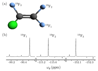
Figure 1: (a) Structure of the molecule, trifluoroiodoethylene, used to realize the three NMR qubits. (b) NMR spectrum of the pseudopure state of the three ¹⁹F qubits.

The rf pulses for pseudopure state preparation Singh et al. (2018c) were designed using the Gradient Ascent Pulse Engineering (GRAPE) technique Khaneja et al. (2005). The duration of the single-qubit gates was around 600 $\mu$s, while for two-qubit gates, the durations of the pulses were set to be around 1/2J, where J is the strength of the scalar coupling between the two relevant qubits. The system was evolved from PPS to other states via state-to-state transfer unitaries, with pulse durations of $\approx 20$ms, and average state fidelities of $\geq 0.99$.

We experimentally prepared states from each of the six inequivalent (under SLOCC) classes of three-qubit states, namely the GHZ state, the W state, three biseparable states (denoted as ‘BS-1’, ‘BS-2’, and ‘BS-3’, respectively) and a separable state (denoted as ‘SEP’), using single-qubit unitary rotations and two-qubit CNOT gates. We chose to use the $|111\rangle$ state as an example of an SEP state and it was prepared by applying a single-qubit rotation of $\pi/2$ on all the three qubits in the initial PPS state. The BS-1 state was prepared by applying an rf pulse inducing a $(-\pi/2)$ rotation with $y$ phase on the second qubit followed by a CNOT₂₃ gate (details of the circuit and corresponding NMR pulse sequence are given in Figure 2). The BS-2 state was prepared by applying a Hadamard gate on the first qubit followed by a CNOT₁₃ gate. Similarly, the BS-3 state was prepared by applying a Hadamard gate on the first qubit followed by a CNOT₁₂ gate and then a $\pi$ rotation of $x$ phase on the first qubit.

The quantum circuit for GHZ state preparation can be found in References Dogra et al. (2015) and Singh et al. (2018a). The W state prepared in the canonical basis was constructed with two controlled-rotation gates and CNOT gates, starting from the PPS state, as shown in Figure 3. The unitaries to be implemented are written inside the boxes representing the gates. The angles $\alpha,\beta$ and $\gamma$ were set to $\alpha=\frac{\pi}{3}$, $\beta=\arcsin{(\frac{1}{\sqrt{3}})}$ and $\gamma=\frac{\pi}{4}$, respectively. The rf pulse durations to implement an angle of $\pi/2$ at power level of 28.59 W is 16.2 $\mu$s.

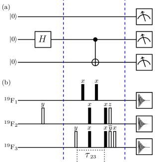
Figure 2: (a) Quantum circuit showing the sequence of implementation of the single-qubit and two-qubit controlled gates required to construct the BS-1 state and (b) the corresponding NMR pulse sequence for the experimental implementation of the BS-1 state. The broad filled rectangles denote $\pi$ pulses and the unfilled rectangles denote $\pi/2$ pulses; the phases of the pulses are written above each pulse. The time interval $\tau_{23}$ is set to $1/2J_{F_{2}F_{3}}$.

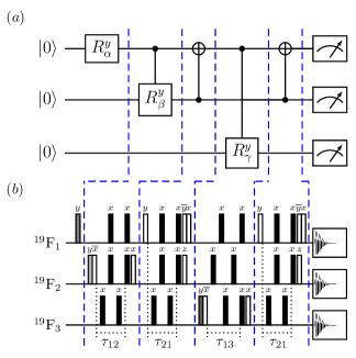
Figure 3: (a) Quantum circuit showing the sequence of implementation of the single-qubit and two-qubit controlled gates required to construct the W state and (b) the corresponding NMR pulse sequence for the experimental implementation of the W state. The broad filled black rectangles denote $\pi$ pulses and the unfilled rectangles denote $\pi/2$ pulses. The three gray rectangles denote the $2\alpha,2\beta$ and $2\gamma$ rotations, where $\alpha=\frac{\pi}{3}$, $\beta=\arcsin{(\frac{1}{\sqrt{3}})}$ and $\gamma=\frac{\pi}{4}$, respectively. The phases of the pulses are written above each pulse. The time interval $\tau_{ij}$ is set to the corresponding $1/2J_{ij}$, where $J_{ij}$ denotes the strength of the coupling between the $i,j$ qubits.

The standard methods for quantum state reconstruction for NMR quantum information processing typically involve performing full state tomography Long et al. (2001); Leskowitz and Mueller (2004) which is computationally expensive, although some alternatives involving maximum likelihood estimation have been proposed and used in our group Singh et al. (2016). For this work, we have used a least squares constrained convex optimization method to reconstruct the density matrix of the desired state Gaikwad et al. . Fidelities of the experimentally reconstructed states (as compared to the theoretically expected state) were computed using the Uhlmann-Jozsa measure Jozsa (1994); Uhlmann (1976):

$${\mathcal{F}}(\chi_{\rm expt},\chi_{{\rm theo}})=\frac{|{\rm Tr}[\chi_{\rm expt}\chi_{\rm theo}^{\dagger}]|}{\sqrt{{\rm Tr}[\chi_{\rm expt}^{\dagger}\chi_{\rm expt}]{\rm Tr}[\chi_{\rm theo}^{\dagger}\chi_{\rm theo}]}}$$ (12)

where $\chi_{{\rm theo}}$ and $\chi_{\rm expt}$ denote the theoretical and experimental density operators, respectively. We experimentally prepared the PPS with a fidelity of 0.96$\pm$0.01. The experimental fidelities for the GHZ and W states were 0.95$\pm$0.01 and $0.93\pm 0.02$, respectively. The BS-1, BS-2, and BS-3 states were prepared with fidelities 0.95$\pm$0.02, 0.95$\pm$0.01, and 0.97$\pm$0.02, respectively, while the fidelity of the SEP state was 0.96$\pm$0.01.

III.2 Reconstructing correlation tensors from NMR observables

The reconstruction of the full correlation tensor (as described in Section II) requires experimentally measuring 27 expectation values of the form $\sigma_{j}\otimes\sigma_{l}\otimes\sigma_{m}$ ($j,l,n=1,2,3$), where $\sigma$ represents the Pauli matrices. For the sake of simplicity, the expectation operators are denoted by combinations of $X,Y,Z$ where $X$ represents the Pauli matrix $\sigma_{x}$ and so on. When the correlation tensors are constructed for any state, some of the expectation values become zero, while others are related to one another. Out of 27 observables needed to construct a correlation matrix, 8 of them become zero in the canonical basis:

$$\langle XXY\rangle = \langle XYX\rangle=\langle XYZ\rangle=\langle XZY\rangle=0$$

$$\langle YXX\rangle = \langle YXZ\rangle=\langle YYY\rangle=\langle YZX\rangle=0$$

Using the following relationships among the expectation values:

$$\langle XXX\rangle = -\langle XYY\rangle=-\langle YXY\rangle=-\langle YYX\rangle$$

$$\langle XXZ\rangle = -\langle YYZ\rangle$$

$$\langle XZX\rangle = -\langle YZY\rangle$$

$$\langle ZXY\rangle = \langle ZYX\rangle$$ (14)

6 of the observables can be computed from the others. This leaves us with the following 13 observables that are required to be experimentally measured:

$$\langle XXX\rangle,\,\,\langle XXZ\rangle,\,\,\langle XZX\rangle,\,\,\langle ZXY\rangle,$$

$$\langle XZZ\rangle,\,\,\langle YZZ\rangle,\,\,\langle ZXX\rangle,\,\,\langle ZXZ\rangle,$$

$$\langle ZYY\rangle,\,\,\langle ZYZ\rangle,\,\,\langle ZZX\rangle,\,\,\langle ZZY\rangle,\,\,\langle ZZZ\rangle$$ (15)

The correlation matrices are computed from 13 expectation values, and are constructed according to Eq. (5). Here $t_{111}^{123}={\rm tr}(\sigma_{1}\otimes\sigma_{1}\otimes\sigma_{1})=\langle XXX\rangle,t_{121}^{123}={\rm tr}(\sigma_{1}\otimes\sigma_{2}\otimes\sigma_{1})=\langle XYX\rangle$ etc. The three correlation matrices are given by:

$$T_{\underline{1}23} = \begin{pmatrix}t_{111}^{123}&0&t_{113}^{123}&0&-t_{111}^{123}&0&t_{131}^{123}&0&t_{133}^{123}\\ 0&-t_{111}^{123}&0&-t_{111}^{123}&0&-t_{113}^{123}&0&-t_{131}^{123}&t_{233}^{123}\\ t_{311}^{123}&t_{312}^{123}&t_{313}^{123}&t_{312}^{123}&t_{322}^{123}&t_{323}^{123}&t_{331}^{123}&t_{332}^{123}&t_{333}^{123}\end{pmatrix}$$

$$T_{\underline{2}13} = \begin{pmatrix}t_{111}^{123}&0&t_{113}^{123}&0&-t_{111}^{123}&0&t_{311}^{123}&t_{312}^{123}&t_{313}^{123}\\ 0&-t_{111}^{123}&0&-t_{111}^{123}&0&-t_{113}^{123}&t_{312}^{123}&t_{322}^{123}&t_{323}^{123}\\ t_{131}^{123}&0&t_{133}^{123}&0&-t_{131}^{123}&t_{233}^{123}&t_{331}^{123}&t_{332}^{123}&t_{333}^{123}\end{pmatrix}$$

$$T_{\underline{3}12} = \begin{pmatrix}t_{111}^{123}&0&t_{131}^{123}&0&-t_{111}^{123}&0&t_{311}^{123}&t_{312}^{123}&t_{331}^{123}\\ 0&-t_{111}^{123}&0&-t_{111}^{123}&0&-t_{131}^{123}&t_{312}^{123}&t_{322}^{123}&t_{332}^{123}\\ t_{113}^{123}&0&t_{133}^{123}&0&-t_{113}^{123}&t_{233}^{123}&t_{313}^{123}&t_{323}^{123}&t_{333}^{123}\end{pmatrix}$$

The ranks of these three correlation matrices are then calculated and the entanglement class is verified according to Table 1. The final step involves quantifying the entanglement by calculating total concurrence given in Eq. (8), using the same experimentally measured set of 13 expectation values.

The schematics of the entanglement classification protocol is shown in Figure 4. The protocol begins with a random state as an input. The black box represents experimental reconstruction of the correlation matrix. The 13 observables are calculated which are shown as inputs to the black box, and the output consists of all the observables not experimentally measured but needed to construct the correlation matrix. The rank of the three correlation matrices obtained for each state are calculated and classified according to Table 1.

Table 2: Ranks and entanglement class characterization of three-qubit experimental states.

State	$R(T_{\underline{1}23})$	$R(T_{\underline{2}31})$	$R(T_{\underline{3}12})$	Class
GHZ	2	2	2	GE
W	3	3	3	GE
BS-1	1	3	3	BS-1
BS-2	3	1	3	BS-2
BS-3	3	3	1	BS-3
SEP	1	1	1	SEP
R1	1	1	1	SEP
R2	1	3	3	BS-1
R3	3	1	3	BS-2
R4	1	1	1	SEP
R5	1	3	3	BS-1
R6	1	1	1	SEP
R7	3	1	3	BS-2
R8	3	3	3	GE
R9	3	3	3	GE
R10	1	3	3	BS-1
R11	3	1	3	BS-2
R12	3	3	1	BS-3
R13	3	1	3	BS-2
R14	3	3	3	GE
R15	3	3	3	GE
R16	3	3	1	BS-3
R17	3	3	3	GE
R18	3	1	3	BS-2
R19	3	3	3	GE
R20	3	3	3	GE

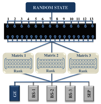
Figure 4: Schematic of the entanglement classification protocol. The blue box at the top represents an unknown pure three-qubit state. The inputs to the black box represent experimental data for the 13 expectation values. The outputs from the black box denote all the expectation values that are required to construct the correlation matrices. All three correlation matrices required for every state make use of these expectation values. The rank of the three correlation matrices are computed to classify the state as belonging to one of the five entanglement classes: Genuinely Entangled (GE), Biseparable (BS-1,BS-2,BS-3), Separable (SEP).

The states that we experimentally constructed from each SLOCC class are:

$${\rm GHZ} = \frac{1}{\sqrt{2}}(|000\rangle+|111\rangle)$$

$${\rm W} = \frac{1}{\sqrt{4}}(|000\rangle+|100\rangle+|101\rangle+|110\rangle)$$

$${\rm BS-}1 = \frac{1}{\sqrt{2}}(|000\rangle+|011\rangle)$$

$${\rm BS-}2 = \frac{1}{\sqrt{2}}(|000\rangle+|101\rangle)$$

$${\rm BS-}3 = \frac{1}{\sqrt{2}}(|010\rangle+|100\rangle)$$

$${\rm SEP} = |111\rangle$$

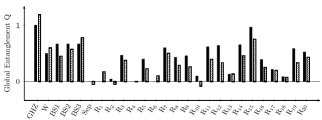
Figure 5: Bar plots of the theoretically expected and the experimentally computed global entanglement $Q(|\psi_{i}\rangle)$ of three-qubit pure states. The horizontal axis labels the state, while the vertical axis represent the global entanglement values. Black and cross-hatched bars represent the theoretical and experimental values, respectively.

The pure states of three qubits were prepared in the canonical basis, which includes the six known states from each SLOCC class as well as arbitrarily prepared random states. The random states were generated using the Mathematica package and the state preparation circuits to prepare the states experimentally were designed using the Mathematica package UniversalQCompiler Wolfram . The pulse circuits thus obtained were implemented experimentally and the states obtained had fidelities in the range 80 to 97$\%$. The experimentally prepared states had several errors due to experimental noise, errors in pulse calibration parameters etc. These errors lead to inaccuracies in the computed expectation values since they are calculated from the experimental matrices. The experimental matrices themselves do not produce exactly zero values of matrix elements where there is zero expected theoretically. Further, since we are finding the rank of the matrix, (the number of independent rows or columns) it is important to be aware of the numerical values. In the known matrices with good fidelity, these “zero errors” were checked and it was found that the values can go up to 0.09. So the error bar was fixed for these values in all the random states in the range $0\pm 0.09$, below which value they can be considered to be zero. The expectation values were calculated from the matrices and were used to construct the correlation matrices labeled $T_{\underline{1}23}$, $T_{\underline{2}31}$, $T_{\underline{3}12}$. The rank of the computed matrices were matched with the theoretical values (Table 1). The ranks of experimentally prepared GHZ, W, BS-1, BS-2, BS-3 and SEP states after error correction match well with the ranks in Table 1, proving the efficacy of the protocol. The ranks of the twenty randomly generated states labeled (R₁,R₂,R₃ etc.. ) were used to classify the states into one of the five entanglement classes (Table 2). The protocol was able to correctly characterize the entanglement class of all the twenty randomly generated states, with no ambiguity.

It is useful in some situations to quantify the amount of entanglement present in the state, and several quantities exist to quantify entanglement. We use concurrence as a measure of entanglement, which is able to quantify entanglement not only in genuinely entangled states but also in biseparable states. We use the same expectation values that we used to classify the states, to measure the entanglement present in them. The global entanglement $Q(|\psi_{i}\rangle)$ for known states was calculated for experimentally obtained states and compared with the theoretically expected values. The results are depicted in Figure 5, where theoretical and experimental results of the computed global entanglement are compared for known states as well as for the randomly generated states. The values of the global entanglement match well with the theoretically expected values, within experimental errors.

IV Conclusions

We designed and experimentally implemented a protocol to classify the entanglement class of and to measure the entanglement in random three-qubit pure states. We reconstructed the correlation tensors experimentally by measuring only a few observables. The ranks of the subsequently computed correlation matrices provide the criteria for classification of multipartite entanglement. The protocol works well for pure states and was experimentally demonstrated on states belonging to the six inequivalent (under SLOCC) classes for three qubits as well as on twenty randomly generated states. The same expectation values that were used to characterize entanglement class of the state, were used to measure the amount of global entanglement present in the state under consideration.

To be able to correctly characterize, certify and detect multipartite entanglement in multiqubit systems using minimal experimental resources is a challenging task and our work is a step forward in this direction. Future work would involve extending the experimental protocol for implementation on larger qubit registers and for mixed states.